Highlights
What are the main findings?
- Multi-temporal clustering using Sentinel-2 data effectively classifies pasture types.
- Dynamic Time Warping (DTW) combined with K-Medoids and hierarchical clustering yields promising results for pasture mapping.
What are the implications of the main findings?
- The OBIA-based clustering framework enables unsupervised pasture type mapping using multi-temporal Sentinel-2 data.
- Biannual change analysis offers insights into pasture stability and the impacts of land management practices.
Abstract
Pasture systems, typically composed of grasses, legumes, and forage crops, are vital livestock nutrition sources. The quality of these pastures depends on various factors, including species composition and growth stage, which directly impact livestock productivity. Remote sensing (RS) technologies offer powerful, non-invasive means for large-scale pasture monitoring and classification, enabling efficient assessment of pasture health across extensive areas. However, traditional supervised classification methods require labelled datasets that are often expensive and labour-intensive to produce, especially over large grasslands. This study explores unsupervised clustering as a cost-effective alternative for identifying pasture types without the need for labelled data. Leveraging spatiotemporal data from the Sentinel-2 mission, we propose a clustering framework that classifies pastures based on their temporal growth dynamics. For this, the pasture segments are first created with quick-shift segmentation, and spectral time series for each segment are grouped into clusters using time-series distance-based clustering techniques. Empirical analysis shows that the dynamic time warping (DTW) distance measure, combined with K-Medoids and hierarchical clustering, delivers promising pasture mapping with normalised mutual information (NMI) of 86.28% and 88.02% for site-1 and site-2 (total area of approx. 2510 ha), respectively, in New South Wales, Australia. This approach offers practical insights for improving pasture management and presents a viable solution for categorising pasture and grazing systems across landscapes.
1. Introduction
Pastures or grasslands are diverse plant communities vital in providing natural forage for livestock such as cattle, sheep, and goats. Maintaining healthy pastures requires effective grazing strategies, including rotational and traditional methods, to support a balanced mix of grasses, legumes, and other forage crops [1]. Beyond cultivated pastures, natural grazing areas such as grasslands and pastoral systems also fulfil livestock feeding needs [2]. Environmental factors, particularly rainfall, significantly influence the productivity of these systems [3]. Pasture management must align with the dietary needs and metabolic traits of specific livestock species to promote optimal grazing conditions and maintain the land’s long-term viability.
Pasture quality is determined mainly by species composition and growth stage [4]. For example, perennial ryegrass is highly valued for its protein content, digestibility, and palatability, making it particularly suitable for dairy cows and other livestock in terms of milk production and weight gain [5]. Identifying the specific type of pasture is therefore crucial for effective management of pastoral ecosystems, as it provides insight into growth rates, which inform decisions about site productivity, optimal stocking rates, and grazing recovery periods [6]. Beyond supplying feed, well-managed pastures contribute to improved soil fertility and structure, help prevent erosion, and enhance grain content by cultivating high-quality forage [7].
Remote sensing (RS) has emerged as a widely used approach for the large-scale identification and classification of pasture types [8]. It offers a non-invasive means of collecting data on pasture growth by measuring the reflectance of energy from vegetation surfaces [3]. Numerous studies have leveraged satellite and aerial RS technologies for monitoring and classifying pastures [9,10]. The moderate resolution imaging spectroradiometer (MODIS) imagery from 2017 and 2018 was used to classify pastures in Brazil into degraded, traditional, and intensified [9]. In another study, object-based image analysis (OBIA) applied to unmanned aerial vehicle (UAV) imagery classified grasslands into four classes—sown biodiverse pasture (SBP), shadow, trees and shrubs, and bare soil—achieving classification accuracy of up to 92% for SBP [10].
However, most existing studies rely on labelled data to train pasture-type classifiers, which are often unavailable and expensive to collect, particularly over vast and remote rangeland areas. Unsupervised clustering offers a practical alternative in such cases, as it does not require labelled samples and can effectively identify similar pasture regions across large landscapes. Pasture clustering offers an efficient way to manage pastures by grouping similar areas based on growth patterns and productivity. This enables land managers and farmers to identify regions suitable for grazing and highlight areas requiring improvement or restoration. For instance, Oleinik et al. [11] applied clustering techniques to multi-temporal normalised difference vegetation index (NDVI) data from the Sentinel-2 mission, successfully identifying three distinct pasture clusters in southern Russia. Nonetheless, clustering pastoral lands remains a complex task due to variations in soil types, vegetation cover, and grazing practices across different regions.
This study introduces a clustering framework that leverages spatiotemporal data from the Sentinel-2 mission to classify pastures based on their temporal growth dynamics. The high temporal resolution (e.g., nominal revisit time of 5 days) of Sentinel-2 time series data captures the subtle changes in landscape and vegetation cover, enabling the detection of pasture dynamics over time. This temporal information allows the clustering framework to group pastures with similar growth patterns into distinct clusters. We assess the performance of various time-series distance-based clustering methods using both internal and external evaluation metrics. The analysis, based on the data collected from two study sites within the Central Tablelands region of New South Wales (NSW), Australia, demonstrates the effectiveness of the proposed clustering framework.
The primary contributions of this work are as follows:
- (i)
- We propose a framework for pasture clustering using spatiotemporal RS data capable of capturing landscape dynamics over extended periods.
- (ii)
- We systematically evaluate clustering methods in conjunction with time-series distance, using both internal and external measures.
- (iii)
- We perform a biannual cluster analysis over six years to examine pasture dynamics and transitions. The analysis reveals that improved pasture and cropping areas experience frequent changes, whereas the native pastures comparatively remain stable.
2. Related Work
RS and OBIA have been widely applied in pasture mapping. In this section, we categorise the existing literature into two main themes: (i) studies that use pixel-based approaches for general grassland and pasture mapping and (ii) studies that incorporate OBIA techniques with RS data to achieve more robust and accurate mapping. Within each thematic discussion, a further division is made based on the use of supervised or unsupervised machine learning for pasture classification.
2.1. Pixel-Based Pasture and Grassland Mapping
The pixel-based approach for RS data analysis is one of the foundational approaches, where each pixel in an RS image, representing a specific ground area, is treated as an individual observation. This method has been widely adopted in pasture mapping, often incorporating data from platforms like Sentinel-2, Landsat, MODIS, and synthetic aperture radar (SAR), alongside ancillary inputs such as climate and management data [6,12,13].
The supervised learning methods have been extensively employed to classify pasture and grassland using multispectral, SAR, hyperspectral, and others, leveraging labelled training data [6,14,15]. Multispectral data from satellite platforms like Sentinel-2 and Landsat have been highly effective for classifying pasture type at moderate spatial resolution. For example, Crabbe et al. [6] employed Sentinel data with k-nearest neighbour (KNN), random forest (RF), and support vector machine (SVM), achieving up to 96% accuracy. Taylor et al. [14] found Landsat data effective for detecting lantana infestations with 85.1% accuracy. SAR data, which is free from clouds, has been investigated by Crabbe et al. [16]. They used Sentinel-1 SAR data to classify C3, C4, and mixed C3/C4 pasture compositions with RF models, which achieved an overall accuracy of 86%. Hyperspectral imaging offers high precision for grassland classification, as reported by Zhao et al. [15], but its high cost and complexity present significant challenges for its widespread application.
Obtaining representative labelled samples for training supervised models in land use and land cover mapping remains a persistent challenge. To address this, several studies attempted to utilise the inherent structure of RS data for pasture identification using unsupervised learning approaches. Seyler et al. [17] implemented a two-stage classification on Landsat imagery, combining unsupervised clustering with spectral profile refinement to distinguish pasture from other vegetation. Stumpf et al. [12] applied stepwise clustering to Landsat time series data to identify grassland management (GM) practice based on biomass productivity and the frequency of management events. Hill et al. [18] utilised RADARSAT-derived textural features with clustering methods to distinguish native from improved pasture covers in Australia and Canada. Santos et al. [19] used MODIS time series data with self-organising maps (SOMs) to reduce data dimensionality and generate initial clusters. These primary clusters were then refined using hierarchical clustering to uncover spatiotemporal land use patterns. Gonçalves et al. [20] utilised Advanced Very High Resolution Radiometer (AVHRR) time series and K-means clustering to identify four distinct land use clusters—agricultural areas, sugarcane fields, urban zones, and forested regions—based on NDVI, albedo, and surface temperature profiles.
In summary, while supervised methods have dominated pixel-based pasture mapping, unsupervised approaches remain limited and are often supplemented with label information at some stages in the pipeline. However, pixel-based methods struggle to capture the inherent complexities of grasslands, as a single pixel does not fully represent the spatial variability and complex interactions within diverse pasture types, making them less effective for mapping heterogeneous pastures.
2.2. OBIA-Based Pasture and Grassland Mapping
OBIA has been particularly effective for differentiating grassland types, as pixel-based classification methods are generally less effective for heterogeneous grasslands and pastures [21,22]. Unlike pixel-based approaches, which treat each pixel in isolation and rely primarily on spectral information, OBIA groups pixels into meaningful image objects and incorporates a broader range of features such as texture, shape, and spatial relationships [10].
Several studies have integrated OBIA with supervised learning methods to enhance pasture mapping. Vilar et al. [10] classified SBP with 92% accuracy, while Lopes et al. [23] utilised OBIA and inter-annual NDVI time series data to classify young and old grasslands. Xu et al. [13] employed OBIA with SVM and RF using multi-season Landsat imagery, digital elevation model (DEM), and vegetation indices, achieving accuracies ranging from 61.4% to 98.71% for grassland type classification. Wu et al. [22] demonstrated that OBIA-based RF outperformed pixel-based methods in semi-arid grassland mapping in Northern China with an overall accuracy of 97.5%. Similarly, Cai et al. [24] found OBIA superior for fractional vegetation cover (FVC) estimation.
Besides the supervised ML techniques, there are very few studies that handle vegetation mapping using unsupervised methods [25]. He et al. [25] utilised the OBIA-based approach with SPOT-5 satellite data to automatically classify the land cover categories in Beijing, China. They extracted the interval structure feature for each segment and performed fuzzy clustering. The post-classification of the resulting clustering images achieved an overall accuracy of 87.24% while classifying the land cover into water, unused land, woodland, grassland, and building.
These studies collectively demonstrate the growing potential of RS, particularly when integrated with multi-source data and machine learning methods, for accurate pasture type classification and mapping. However, the reliance on labelled samples to train supervised classifiers remains a major challenge, as it requires costly and labour-intensive data collection, limiting the applicability of these methods for large-scale rangeland applications.
The review of existing work echoes the motivation behind this study, where we introduce an unsupervised framework that leverages the spatiotemporal dynamics through OBIA and clustering techniques. This clustering framework enables pasture mapping into native and improved categories based on their inherent spectral–temporal profiles, rather than relying on pre-labelled pasture types.
3. Materials and Methods
3.1. Study Area
This study focuses on two pasture farms—site-1 (with an area of approx. 920 ha) and site-2 (with an area of approx. 1590 ha)—located within the Central Tablelands region in the state of NSW, Australia (Figure 1). Australia is known for its extensive grasslands and pasture systems; NSW is no exception. Within NSW, the Central Tablelands region plays a significant role in the state’s agricultural production, supporting a diverse range of farming enterprises. The primary industries in this region include livestock grazing, mainly sheep and cattle, and broadacre cropping [26]. The landscape primarily comprises native and improved pastures, supplemented by canola, barley, and other grains cultivated mainly for livestock feed. Other agricultural activities involve the production of vegetables, pome and stone fruits, wine and table grapes, and nursery plants such as cut flowers [27]. The region experiences a temperate climate characterised by cool winters, warm summers, and relatively uniform rainfall throughout the year [28].
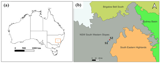
Figure 1.
Study area map: (a) state boundary map of Australia, and (b) the study site-1 (S1) and site-2 (S2) on the bioregion area map [29].
3.2. Satellite Image Time Series (SITS) Data
We obtained RS data from Digital Earth Australia (DEA) https://www.ga.gov.au/scientific-topics/dea (accessed on 24 January 2025), a data cube platform that provides analysis-ready data (ARD) for the Australian continent. We used Sentinel-2 (A/B) imagery as our baseline dataset. DEA pre-processes the European Space Agency’s Sentinel-2 MSI imagery using Nadir-corrected Bidirectional Reflectance Distribution Function Adjusted Reflectance (NBART) to correct inconsistencies across land and coastal areas [30].
For our study areas, we extracted Sentinel-2 images with less than 10% cloud cover, as determined by the s2cloudless algorithm [31]. The selected bands included visible BGR (B2, B3, B4), red-edge (B5, B6, B7), near-infrared (B8, B8a), and shortwave infrared (B11, B12). To ensure the spatial consistency across all spectral bands, they were resampled to a uniform 10 m spatial resolution. Figure 2 presents the distribution of Sentinel-2 images from 2017 to 2024, revealing a decrease in available imagery during months with higher rainfall. This is likely due to increased cloud cover, resulting in more images being filtered out by the cloud masking process. For example, from July to November 2022, image availability was low for both sites, coinciding with rainfall levels of approximately 200 mm.
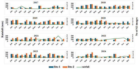
Figure 2.
Monthly summary of Sentinel-2 (S2) images for study sites (site-1 and site-2) with rainfall (data accessed form [28]) from 2017 to 2024.
3.3. Normalised Difference Vegetation Index (NDVI)
The normalised difference vegetation index (NDVI) is a widely used proxy for assessing vegetation vigour (greenness) and biomass in both crops and pastures [10]. It has been effectively applied to distinguish between degraded and healthy pastures [32] and to differentiate pastures from tree-covered areas [10], among other classifications. Building on its proven effectiveness in pasture analysis, we incorporated NDVI as a temporal input in our framework to segment pasture areas based on their spatiotemporal dynamics. NDVI values for the study period were calculated using the Sentinel-2 imagery time series (SITS), derived from the near-infrared (B8) and red (B4) bands, as defined in Equation (1).
3.4. Proposed Framework for OBIA-Based Pasture Clustering
Figure 3 illustrates the proposed multi-step OBIA-based pasture clustering framework. The initial pre-processing involved cloud masking, smoothing, and monthly compositing to reduce noise from residual cloud cover. Next, pixel-based segmentation was performed using NDVI data derived from eight years of Sentinel-2 imagery, grouping similar pixels into homogeneous pasture segments (also referred to as pasture objects). Mean zonal statistics from ten bands of Sentinel-2 SITS were then extracted for each pasture object to construct multivariate time series. These features were then used in computing time series distance metrics, followed by clustering algorithms. The subsequent sections describe each step of the framework in detail.
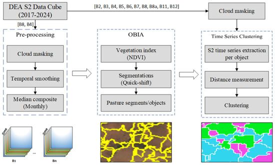
Figure 3.
The OBIA–based pasture clustering framework. Note: B2, B3, B4, etc., represent the Sentinel-2 bands extracted from DEA.
3.4.1. Pre-Processing
This section outlines the pre-processing steps involved in creating the RS data cubes. The first data cube was built to store NDVI time series data spanning eight years (2017–2024). To construct this NDVI data cube, we began by extracting the red (B4) and near-infrared (B8) bands from the SITS and computed NDVI values using Equation (1). As minimal pre-processing, temporal smoothing was applied to the Sentinel-2 bands (B4 and B8) time series using a simple moving average (SMA) with a window size of 4 (approximately 20 to 30 days). This window size was chosen to reduce short-term noise, typically caused by cloud cover and atmospheric effects, while preserving the main vegetation trends. Following smoothing, a monthly median composite was calculated from the smoothed data to produce the final NDVI data cube. This data cube then served as the input for image segmentation, generating homogeneous pasture segments based on their eight-year NDVI time series profiles.
3.4.2. Segmentation for Pasture Landscape Formation
OBIA, which employs segmentation techniques to group similar pixels into superpixels, has become a widely used approach for contextual analysis in RS [33]. Superpixels provide richer information than individual pixels by aggregating adjacent pixels with similar spectral, textural, or spatial characteristics into larger and more meaningful regions. Unlike traditional pixel-based methods, which are often sensitive to spectral noise, superpixel-based analysis enables the application of dynamic, rule-based recognition strategies, leading to a more comprehensive and robust interpretation of satellite imagery [21,34]. Additionally, this approach can significantly reduce the computational burden associated with processing large-scale RS datasets [35].
Segmentation is the first step in any OBIA-based SITS classification or clustering task. In this study, we adopted the quick-shift algorithm [36], available in the scikit-image package [37]. Quick-shift’s mode-seeking approach efficiently groups pixels based on both colour and spatial proximity, making it well-suited for segmenting NDVI time-series data into spatially coherent and vegetatively homogeneous units. This is particularly important in our context, where the goal is to delineate meaningful pasture objects from multi-temporal vegetation dynamics. Since the focus of this study is on time series clustering, rather than on evaluating the segmentation techniques, quick-shift was selected as a suitable baseline. However, the proposed pipeline is flexible and can incorporate any segmentation method that produces spatially homogeneous objects from the SITS. To create the pasture object through segmentation, we utilised the NDVI data of a long period (2017–2024), aiming to obtain the homogeneous vegetative area that corresponds to a meaningful pasture landscape. Specifically, the segmentation methods partition the spatial domain of NDVI data S into n non-overlapping spatial units, , referred to as pasture objects (Equation (2)).
3.4.3. Time Series Extraction and Similarity Measurement
Following the creation of pasture objects through image segmentation in the previous step, we constructed a multivariate time series (MTS) for each pasture object using ten spectral bands of Sentinel-2, to serve as input to the subsequent cluster analysis. This process involves aggregating pixel-level spectral information from Sentinel-2 spectral bands over the defined study period (annual season of pasture) using an average of the radiometric value of pixels in the associated segment [38].
Mathematically, let Sentinel-2 SITS of m images be represented as
where each denotes a multi-spectral image at time t with … and representing pixel coordinates with an image of spatial dimension and representing the spectral band index.
From this spatiotemporal dataset D, we derive the multivariate time series for each segment , computed as in Equation (4).
Here, represents the multivariate time series of object with each row corresponding to a time step and each column to a spectral band.
Next, we evaluate the similarity between MTS of different pasture objects using three distance measures: Euclidean distance (ED) [4] and Dynamic Time Wrapping (DTW) [39]. These distances were selected due to their complementary strength and proven relevance in time series analysis, as evidenced by their consistent performance across a broad range of time series data mining tasks [40,41,42].
ED is commonly used due to its simplicity and computational efficiency. It measures the straight-line distance between two time series and , assuming equal length, as defined in Equation (5).
Unlike ED, DTW is a flexible metric for comparing time series that may vary in time. It finds the optimal alignment between two sequences by minimising the cumulative distance over all possible warping paths. The DTW distance between two time series and can be defined as in Equation (6) [42].
where represents the set of admissible warping paths and represents the pairwise distance (e.g., Euclidean) at each aligned step , typically computed via dynamic programming [42].
3.4.4. Clustering
The final step of the framework is clustering, where pasture segments exhibiting similar temporal dynamics are grouped based on a chosen distance metric. For this study, three clustering algorithms are employed: K-Means (KM), Partition Around Medoids (PAM), and Hierarchical Clustering (HC). These methods are selected due to their compatibility with time series distance measures such as DTW and Euclidean (Section 3.4.3). We utilise tslearn [43], sklearn-extra [44], and sklearn [45] to implement time series KM, PAM, and HC, respectively.
KM is widely favoured for its computational efficiency and scalability [46]. It requires the computation of centroids, and the method for determining these cluster centroids depends on the distance metrics employed. When using ED, centroids are derived as the standard mean of the time series. In contrast, for DTW, centroids are derived through barycenter averaging, which more effectively preserves the temporal alignment across sequences [47].
PAM, also known as K-Medoids, is similar to KM but uses the actual data points as cluster centres instead of centroids, minimising the total intra-cluster distance. By selecting medoids from the dataset, PAM offers better interpretability and is less sensitive to outliers [48].
HC is a bottom-up agglomerative clustering method that iteratively merges the closest clusters based on a specified distance metric and linkage criterion. It starts with each data point as an individual cluster and progressively merges clusters until all points form a single cluster. This results in a tree-like dendrogram, illustrating the merging steps. Unlike KM and PAM, it does not require prior knowledge of the number of clusters. The optimal number of clusters can be inferred using the longest vertical distance in the dendrogram.
3.5. Reference Data
As ground truth labels for pasture segments are not directly available, direct evaluation is not possible. Instead, we adopt an indirect validation approach using publicly available land use (LU) reference data. Specifically, we leverage the Catchment Scale Land Use of Australia (CLUM) dataset, developed by the Australian Bureau of Agricultural and Resource Economics and Sciences (ABARES). This dataset integrates vector-based land use data from state and territory mapping programs under the Collaborative Land Use and Management Program (CLUM) [49]. CLUM provides land use information at a 50 m resolution, classified according to the Australian Land Use and Management scheme. For this study, we retained only relevant categories—cropping, grazed native pasture, and grazed improved pasture—masking out all other classes. To ensure spatial consistency, the CLUM dataset is resampled to 10m resolution using nearest neighbour (NN) interpolation to match the resolution of Sentinel-2 imagery. All the datasets used in this study are projected into a common coordinate reference system (EPSG:3577; GDA/Australian Albers).
3.6. Evaluation Metrics
We utilise two kinds of evaluation metrics: internal and external. First, the internal evaluation metrics measure the cluster’s quality without needing any ground truth references. Specifically, we choose the silhouette coefficient (SC) (Equation (7)).
where and represent the mean distance from to all points in its own cluster (intra-cluster) and mean distance between and all other points in the next nearest cluster (inter-cluster), respectively. For a silhouette score, larger values are better, with +1 meaning well-separated clusters, 0 meaning overlapping clusters, and negative values meaning likely misclassification.
For external evaluation which requires ground truth pasture labels, we choose the Adjusted Rand Index (ARI) (Equation (8)), Fowlkes–Mallows Index (FMI) (Equation (9)), Normalized Mutual Information (NMI) (Equation (10)), and Purity (Equation (11)). These evaluation metrics measure the consensus between external and cluster labels. Most of them range from 0 (no agreement) to 1 (perfect agreement), except ARI, which can range from −1 to 1.
where is the rand index.
where , , , and represent true positive, true negative, false positive, and false negative.
where represents the mutual information between U (true label assignment) and V (predicted cluster assignment) derived from the joint probabilities between the true (external) label assignment (U) and predicted cluster assignment (V), and and represent the “Entropy” of U and V, respectively.
where and represent the set of points in cluster i and true class j. Additionally, n represents the total number of samples in the dataset, and k is the total number of clusters.
4. Results and Discussion
This section presents the data size and analyses the clustering results. The sample size of the time series dataset is determined by the number of pure segments listed in Table 1.

Table 1.
Statistics of final pasture segments for each study site using the quick-shift method.
For example, there are 457 multivariate time series, each with 10 variables (ten Sentinel-2 bands) for site-1, considering only pure segments. The full Sentinel-2 temporal resolution is considered for each time series. The entire study period (2017–2024) is divided into biannual subsets: 2017–2018 (D1), 2019–2020 (D2), 2021–2022 (D3), and 2023–2024 (D4). This time window is chosen because the study sites include perennial native pastures that grow continuously for more than a year. We first evaluate the clustering framework using the subset D1 (2017–2018) with both external and internal evaluation metrics, as these dates closely align with the update date (2017) of the CLUM dataset for the study sites https://www.agriculture.gov.au/abares/aclump/land-use/catchment-scale-land-use-and-commodities-update-2023 (accessed on 3 February 2025). Then, we present the biannual cluster change analysis using subsets D2, D3, and D4.
4.1. Segmentation Results and Pure Segments
The segmentation results from quick-shift (Figure 4) illustrate that the segments appear more uniform and better aligned with the underlying pasture landscape, reflecting the homogeneous vegetative dynamics over time in the study site. For evaluation purposes, uniformly labelled segments were created by overlaying the resulting segmentation map with the CLUM raster. A reference label (e.g., native pasture, improved pasture, or crop) was assigned to a segment only if all pixels within that segment had the same label in the CLUM raster, ensuring label consistency within each selected segment. The segments labelled as mixed pasture are excluded from the performance evaluation because they contain noisy labels. The numbers of total segments and corresponding pure segments for each study site are reported in Table 1 and illustrated in Figure 5.
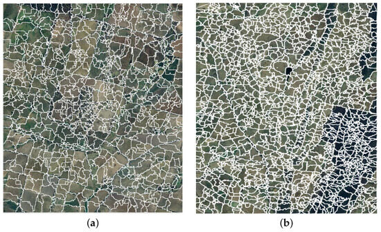
Figure 4.
Pasture segments (in white) generated by quick-shift for (a) site-1 and (b) site-2, where the high-resolution images from Google Satellite (© 2023) are used for visualisation purposes only. Note that, to maintain the layout consistency, the images are not shown to scale.
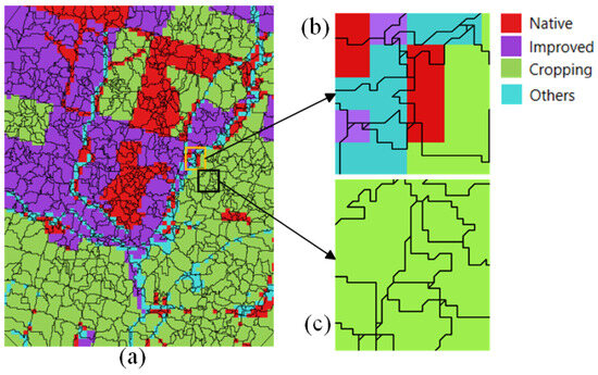
Figure 5.
Illustration of selecting pure segments as reference segments from the segmentation results: (a) all segments overlaid over the CLUM raster, (b) zoomed-in view showing examples of mixed segments, and (c) zoomed-in view showing samples of pure segments.
4.2. Cluster Evaluation Using Silhouette Analysis
Silhouette analysis evaluates the compactness and separation of clusters without relying on ground truth labels and is commonly used to assess the optimal number of clusters (k). To explore this, we ran KM, PAM, and HC with values of k ranging from 2 to 4 for both site-1 and site-2.
For site-1 (Figure 6), the SC reaches its highest value for k = 2 and gradually decreases for k = 3 and k = 4 across all distance metrics and clustering methods. Specifically, for k = 2, DTW achieves SC in the range of 0.38–0.40, whereas ED yields slightly lower SC, ranging from 0.35 to 0.37. As k increases to 3 and 4, the clusters become less compact, as indicated by lower SC, particularly for KM and HC. However, the PAM maintains slightly higher SC scores for k = 3, suggesting improved clustering quality compared to KM and HC. Based on Silhouette analysis, the optimal number of clusters for site-1 is likely k = 2 or k = 3, as a further increase in k leads to a consistent decline in SC across all clustering methods and distance metrics.

Figure 6.
Silhouette coefficient (SC) for site-1 with (a) KM, (b) HC, and (c) PAM clustering for D1 (2017–2018). Note: ’k’ represents the number of clusters.
Similarly, for site-2 (see Figure 7), the SC exhibits a consistent decline as the number of clusters k increases from 2 to 4 across all clustering methods (KM, HC, and PAM) and both distance metrics (DTW and ED). The highest SC values are observed at k = 2, where DTW generally yields better performance compared to ED across most methods. Here, the SC falls within a higher range (0.56–0.66) for all clustering methods, with DTW slightly outperforming ED. As K increases to 3, a moderate drop in SC is observed, with SCs falling into a mid-range (0.30–0.49), across all clustering methods. PAM tends to maintain better cluster compactness than KM and HC for k = 3. However, when k = 4, SC declines further, entering a lower range that reflects diminished clustering quality across all methods.

Figure 7.
Silhouette coefficient (SC) for site-2 with (a) KM, (b) HC, and (c) PAM clustering for D1 (2017–2018). Note: ’k’ represents the number of clusters.
Compared to site-1, the SCs for site-2 are generally higher across all clustering methods and distance metrics, especially at k = 2 and k = 3. For instance, site-2 has SC values of 0.6646 when using KM, with DTW outperforming its counterparts for site-1 (KM with DTW only has an SC of 0.3994). This indicates that the clustering structures in site-2 are more compact and well separated, especially when using DTW as the distance metric. PAM consistently demonstrates strong performance across both sites, suggesting its robustness to temporal dynamics. This might be due to the PAM’s reduced sensitivity to outliers and noise, as it uses actual data points as cluster centres, making it more resilient to the fluctuations observed in pasture growth and senescence. Overall, the optimal number of clusters for site-2 is again likely k = 2 or k = 3, supported by the consistently highest SC value across all methods.
4.3. Cluster Analysis with External Labels
In this section, the clustering results are reported in terms of external evaluation measures: ARI, NMI, FMI, and Purity (Section 3.6). As inferred from silhouette analysis, all cluster methods are evaluated for k = 2 and k = 3. For k = 2, improved vs. native pasture segments are considered as reference labels, whereas cropping is added for k = 3.
While looking at Table 2 for the two-cluster scenario (i.e., k = 2), the results indicate that DTW as a distance metric consistently outperforms ED across all clustering algorithms.

Table 2.
Comparison of distance measures across study sites and clustering methods for two clusters (k = 2) on D1 (2017–2018). Bold values denote the highest performance.
For site-1, the highest performance was achieved by PAM with DTW, which attained the highest ARI (0.7261), NMI (0.6246), FMI (0.8628), and Purity (0.9264). This is closely followed by HC with DTW, which also showed strong results across all metrics. In contrast, KM with either distance metric yielded slightly lower performance, though still within acceptable ranges, indicating moderate agreement with ground truth labels. Similarly, for site-2, HC with DTW demonstrates the best performance among all methods. It achieved the highest ARI (0.7494), NMI (0.6372), FMI (0.8802), and Purity (0.9330).
While faster and simpler, KM lagged slightly behind in both sites, particularly when using ED. For both sites, clustering with ED led to consistently lower scores, especially in ARI and NMI, which are more sensitive to cluster structure alignment with true labels. In summary, the clustering results with DTW distance measures are slightly better than ED across all methods, while PAM and HC offer better alignment with the reference label compared to KM. More importantly, the overall trend is consistent across both site-1 and site-2, suggesting the robustness of these methods across different datasets.
For the three-cluster case (k = 3), distinguishing between improved pasture, native pasture, and cropping, the clustering results show modest clustering performance overall, with noticeable variations depending on the clustering algorithm, distance measure, and study site (Table 3). For site-1, the best performance is achieved using HC with DTW, which produced relatively higher scores for NMI and purity compared to other combinations, indicating better cluster–label alignment. However, KM with DTW also performed comparably, suggesting that DTW as a distance metric provides more informative temporal similarity than ED, regardless of the clustering algorithm. In contrast, for site-2, clustering quality is generally higher, particularly for HC and PAM with ED. HC with ED achieved the highest ARI (0.5430), NMI (0.5286), FMI (0.7322), and purity (0.7082), while other combinations also performed well across the study sites.

Table 3.
Comparison of distance measures across study sites and clustering methods for three clusters (k = 3) on D1 (2017–2018). Bold values denote the highest performance.
Comparing the two sites, site-2 consistently yielded higher ARI, NMI, and FMI scores, indicating a stronger and more separable cluster structure in the time series data. Additionally, DTW outperformed ED in the majority of the configurations, suggesting that it can capture the nuanced temporal dynamics of different pasture types. For instance, native and improved pasture exhibit distinct phenological behaviours due to variations in their growth cycles, response to environmental conditions, and other factors. The ability of DTW to align time series with a temporal shift makes it particularly effective for measuring phenological differences between these pasture types.
4.4. Qualitative Analysis of Clustering Results
A qualitative evaluation of clustering results for the three-cluster case (k = 3) is presented in Figure 8 and Figure 9, corresponding to site-1 and site-2, respectively. To generate these qualitative maps, we utilise the clustering output from the highest-performing models based on NMI using the results in Table 3 as it measures the direct alignment between true and predicted labels.
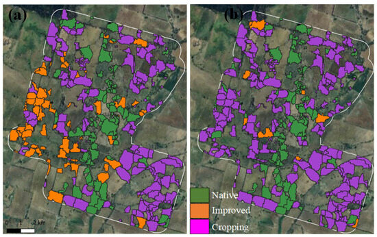
Figure 8.
The pasture type clustering result maps (using HC with DTW) for site-1 with (a) LU labels and (b) pasture clusters (the white line shows the farm boundary).
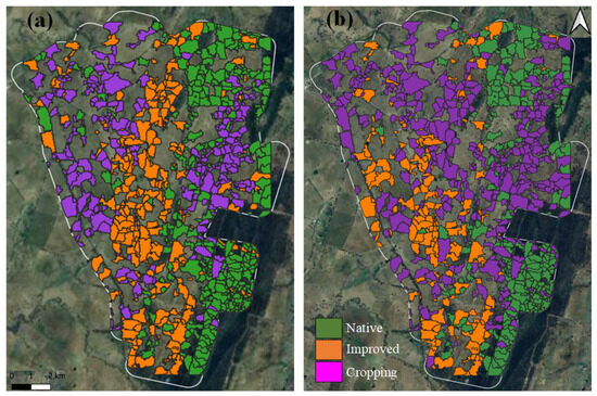
Figure 9.
The pasture type clustering result maps (using HC with ED) for site-2 with (a) LU labels and (b) pasture clusters (the white line shows the farm boundary).
For site-1 (Figure 8), the native pastures are most correctly aligned with reference labels compared to improved pasture and cropping. Here, the improved pasture and cropping areas are misclassified, possibly due to their overlapping temporal signatures.
For site-2 (Figure 9), visual comparison with the reference pasture type reveals that most native and improved pasture segments are well-aligned with their corresponding reference labels. However, cropping areas are again frequently misclassified as improved pasture in the resulting cluster maps here.
The results highlight that native pastures are easy to distinguish from other land types, as they follow more consistent growth patterns. In contrast, cropping and improved pasture are challenging to differentiate based on spectral–temporal profiles. Nevertheless, classifying pasture into native vs. improved categories can provide valuable insight for farm management. For example, by understanding these distinctions, farmers can optimise grazing management, improve resource allocation, and implement strategies that balance short-term productivity with long-term ecological resilience.
4.5. Biannual Cluster Change Analysis
The clustering framework was applied to biannual time series of Sentinel-2 spectral bands over six years (2019–2024) to assess the vegetation changes in cluster segments for site-1 and site-2. The resulting clustering maps, presented in Figure 10 and Figure 11, illustrate temporal variations in cluster assignments, offering insights into underlying pasture dynamics.
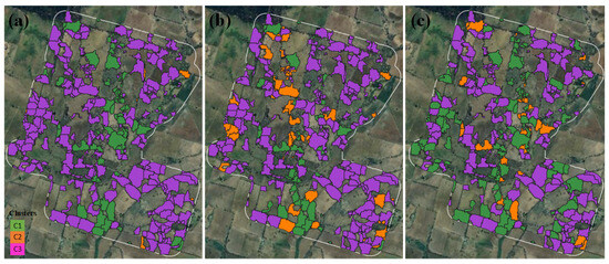
Figure 10.
The clustering maps of site-1 for biannual time series of (a) 2019–2020 (D2), (b) 2021–2022 (D3), and (c) 2023–2024 (D4). Note that ’C1’, ’C2’, and ’C3’ correspond to legends for clusters 1, 2, and 3, respectively.
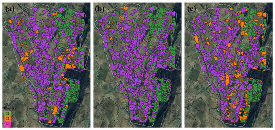
Figure 11.
The clustering maps of site-2 for biannual time series of (a) 2019–2020, (b) 2021–2022, and (c) 2023–2024. Note that ’C1’, ’C2’, and ’C3’ correspond to legends for clusters 1, 2, and 3, respectively.
Notably, the native pasture cluster () remains relatively stable over time across both sites, which is consistent with ecological expectations as native pasture typically comprises perennial grass and shrubs. These communities are generally less intensively managed and thus exhibit lower spectral variability over time, especially in the absence of major disturbances such as fire and landslides.
In contrast, the improved pasture () and cropping () clusters show more frequent transitions between time intervals across both sites. For example, in site-1, a notable number of segments classified as in 2021–2022 are re-clustered as by 2023–2024. Such transitions may be indicative of land management decisions, including the conversion of pasture to annual cropping or variation in forage availability driven by seasonal rainfall, grazing pressure, and sowing schedules. Improved pasture systems, which often involve fertilised or reseeded pasture species, are subject to active management, leading to changes in phenology that are detectable in spectral signatures.
In cropping areas, the observed changes may be due to annual cropping cycles, where distinct seasonal phenology and fallow periods introduce substantial inter-annual spectral differences. The confusion between improved pasture and cropping clusters is likely due to overlapping spectral–temporal signatures, especially in those systems where cropping and pasture are integrated or rotated in short time frames.
5. Conclusion and Future Work
In this study, we proposed an OBIA-based framework for pasture clustering using temporal Sentinel-2 imagery, aimed at capturing and assessing vegetation landscape changes over time. The framework incorporates a detailed comparison of clustering methods and time-series distance measures, evaluated through external and internal validation metrics. Additionally, our analysis of biannual clustering patterns over six years reveals notable shifts in landscape dynamics, providing valuable insights into long-term pasture variability and land management impacts.
In summary, our study demonstrates the potential of an OBIA-based clustering framework using multi-temporal SITS, effectively capturing the temporal variability of pasture growth. However, it has two main limitations. First, it relies solely on Sentinel-2 SITS, which might limit the diversity of information. Second, the use of the pure segments approach, which excludes the mixed segments, may introduce bias towards clearly defined pasture areas. Future work should focus on integrating additional data sources, such as climatic and topographic variables, and extending the analysis to incorporate finer temporal and spatial resolutions would allow for a more detailed understanding of seasonal dynamics and localised changes within pasture ecosystems.
Author Contributions
Conceptualization: T.B.S., R.N., J.P.G. and K.S.; methodology: T.B.S., R.N., A.W. and K.S.; software: T.B.S.; validation, T.B.S., R.N., A.W. and J.P.G.; formal analysis: T.B.S., R.N., A.W., J.P.G. and K.S.; investigation: T.B.S.; resources: R.N. and K.S.; writing—original draft preparation: T.B.S.; writing—review and editing: T.B.S., R.N., A.W., J.P.G. and K.S.; supervision: R.N., A.W., J.P.G. and K.S.; project administration: R.N. and K.S.; funding acquisition: R.N. All authors have read and agreed to the published version of the manuscript.
Funding
This research was supported by funding from Food Agility CRC Ltd., funded under the Commonwealth Government CRC Program. The CRC Program supports industry-led collaborations between industry, researchers, and the community. This research was also partially supported by funding from Meat and Livestock Australia (MLA). The funders had no role in the study design, data collection, analysis, interpretation of results, writing of the manuscript, or decision to submit for publication.
Data Availability Statement
All data used in the manuscript will be made available upon reasonable request and subject to confidentiality restrictions.
Acknowledgments
The authors would like to acknowledge Peter Scarth from CIBO Lab for his valuable suggestions and expert feedback during the preparation of this manuscript.
Conflicts of Interest
Author Kenneth Sabir is an employee of AgriWebb Pty Ltd. The remaining authors declare no conflict of interest.
Abbreviations
The following abbreviations are used in this manuscript:
| ABARES | Australian Bureau of Agricultural and Resource Economics and Science |
| ARD | Analysis-Ready data |
| ARI | Adjusted rand index |
| AVHRR | Advanced Very High Resolution Radiometer |
| BGR | Blue Green Red |
| CLUM | Catchment Scale Land Use of Australia |
| DEA | Digital Earth Australia |
| DEM | Digital elevation model |
| DTW | Dynamic Time Warping |
| ED | Euclidean Distance |
| FMI | Fowlkes–Mallows Index |
| GM | Grassland Management |
| kNN | k-Nearest Neighbour |
| MODIS | Moderate Resolution Imaging Spectroradiometer |
| MTS | Multivariate Time Series |
| NDVI | Normalised Difference Vegetation Index |
| NBART | Nadir-corrected Bidirectional Reflectance Distribution Function Adjusted Reflectance |
| NMI | Normalized Mutual Information |
| OBIA | Object-based Image Analysis |
| RF | Random Forest |
| RS | Remote Sensing |
| SAR | Synthetic Aperture Radar |
| SITS | Satellite image time series |
| SMA | Simple Moving Average |
| SOM | Self-organising maps |
| SVM | Support Vector Machine |
| SBP | Sown Biodiverse Pasture |
References
- Wróbel, B.; Zielewicz, W.; Staniak, M. Challenges of pasture feeding systems—Opportunities and constraints. Agriculture 2023, 13, 974. [Google Scholar] [CrossRef]
- Horn, J.; Isselstein, J. How do we feed grazing livestock in the future? A case for knowledge-driven grazing systems. Grass Forage Sci. 2022, 77, 153–166. [Google Scholar] [CrossRef]
- Scarth, P.; Röder, A.; Schmidt, M.; Denham, R. Tracking grazing pressure and climate interaction-the role of Landsat fractional cover in time series analysis. In Proceedings of the 15th Australasian Remote Sensing and Photogrammetry Conference, Alice Springs, Australia, 13–17 September 2010; Volume 13. [Google Scholar]
- Adar, S.; Sternberg, M.; Argaman, E.; Henkin, Z.; Dovrat, G.; Zaady, E.; Paz-Kagan, T. Testing a novel pasture quality index using remote sensing tools in semiarid and Mediterranean grasslands. Agric. Ecosyst. Environ. 2023, 357, 108674. [Google Scholar] [CrossRef]
- Fulkerson, B. Perennial ryegrass. In Future Dairy; University of Sydney: Camperdown, Australia, 2007. [Google Scholar]
- Crabbe, R.A.; Lamb, D.; Edwards, C. Discrimination of species composition types of a grazed pasture landscape using Sentinel-1 and Sentinel-2 data. Int. J. Appl. Earth Obs. Geoinf. 2020, 84, 101978. [Google Scholar] [CrossRef]
- Monjardino, M.; Loi, A.; Thomas, D.T.; Revell, C.K.; Flohr, B.M.; Llewellyn, R.S.; Norman, H.C. Improved legume pastures increase economic value, resilience and sustainability of crop-livestock systems. Agric. Syst. 2022, 203, 103519. [Google Scholar] [CrossRef]
- Shahi, T.B.; Balasubramaniam, T.; Sabir, K.; Nayak, R. Pasture monitoring using remote sensing and machine learning: A review of methods and applications. Remote Sens. Appl. Soc. Environ. 2025, 101459. [Google Scholar] [CrossRef]
- Bonamigo, A.; Oliveira, J.D.C.; Lamparelli, R.; Figueiredo, G.; Campbell, E.; Soares, J.; Monteiro, L.; Vianna, M.; Jaiswal, D.; Sheehan, J.; et al. Mapping Pasture Areas In Western Region Of SÃO Paulo State, Brazil. In Proceedings of the 2020 IEEE Latin American GRSS & ISPRS Remote Sensing Conference (LAGIRS), Santiago, Chile, 22–26 March 2020; pp. 681–686. [Google Scholar]
- Vilar, P.; Morais, T.G.; Rodrigues, N.R.; Gama, I.; Monteiro, M.L.; Domingos, T.; Teixeira, R.F. Object-based classification approaches for multitemporal identification and monitoring of pastures in agroforestry regions using multispectral unmanned aerial vehicle products. Remote Sens. 2020, 12, 814. [Google Scholar] [CrossRef]
- Oleinik, S.; Lesnyak, T.; Skripkin, V.; Litvin, D. Remote clustering of pastures. In Proceedings of the BIO Web of Conferences; EDP Sciences: Les Ulis, France, 2024; Volume 82, p. 05033. [Google Scholar]
- Stumpf, F.; Schneider, M.K.; Keller, A.; Mayr, A.; Rentschler, T.; Meuli, R.G.; Schaepman, M.; Liebisch, F. Spatial monitoring of grassland management using multi-temporal satellite imagery. Ecol. Indic. 2020, 113, 106201. [Google Scholar] [CrossRef]
- Xu, D.; Chen, B.; Shen, B.; Wang, X.; Yan, Y.; Xu, L.; Xin, X. The classification of grassland types based on object-based image analysis with multisource data. Rangel. Ecol. Manag. 2019, 72, 318–326. [Google Scholar] [CrossRef]
- Taylor, S.; Kumar, L.; Reid, N. Accuracy comparison of Quickbird, Landsat TM and SPOT 5 imagery for Lantana camara mapping. J. Spat. Sci. 2011, 56, 241–252. [Google Scholar] [CrossRef]
- Zhao, X.; Zhang, S.; Shi, R.; Yan, W.; Pan, X. Classification of grassland conditions using a hyperspectral camera and deep learning. Int. J. Remote Sens. 2025, 46, 1–21. [Google Scholar] [CrossRef]
- Crabbe, R.A.; Lamb, D.W.; Edwards, C. Discriminating between C3, C4, and mixed C3/C4 pasture grasses of a grazed landscape using multi-temporal Sentinel-1a data. Remote Sens. 2019, 11, 253. [Google Scholar] [CrossRef]
- Seyler, F.; Chaplot, V.; Muller, F.; Cerri, C.; Bernoux, M.; Ballester, V.; Feller, C.; Cerri, C. Pasture mapping by classification of Landsat TM images. Analysis of the spectral behaviour of the pasture class in a real medium-scale environment: The case of the Piracicaba Catchment (12,400 km2, Brazil). Int. J. Remote Sens. 2002, 23, 4985–5004. [Google Scholar] [CrossRef]
- Hill, M.; Smith, A.; Foster, T. Remote sensing of grassland with RADARSAT; case studies from Australia and Canada. Can. J. Remote Sens. 2000, 26, 285–296. [Google Scholar] [CrossRef]
- Santos, L.A.; Ferreira, K.; Picoli, M.; Camara, G.; Zurita-Milla, R.; Augustijn, E.W. Identifying spatiotemporal patterns in land use and cover samples from satellite image time series. Remote Sens. 2021, 13, 974. [Google Scholar] [CrossRef]
- Gonçalves, R.R.d.V.; Zullo, J.; Amaral, B.; Coltri, P.P.; Sousa, E.P.M.d.; Romani, L.A.S. Land use temporal analysis through clustering techniques on satellite image time series. In Proceedings of the 2014 IEEE Geoscience and Remote Sensing Symposium, Quebec City, QC, Canada, 13–18 July 2014; pp. 2173–2176. [Google Scholar]
- Whiteside, T.G.; Boggs, G.S.; Maier, S.W. Comparing object-based and pixel-based classifications for mapping savannas. Int. J. Appl. Earth Obs. Geoinf. 2011, 13, 884–893. [Google Scholar] [CrossRef]
- Wu, N.; Crusiol, L.G.T.; Liu, G.; Wuyun, D.; Han, G. Comparing machine learning algorithms for pixel/object-based classifications of semi-arid grassland in northern China using multisource medium resolution imageries. Remote Sens. 2023, 15, 750. [Google Scholar] [CrossRef]
- Lopes, M.; Fauvel, M.; Girard, S.; Sheeren, D. Object-based classification of grasslands from high resolution satellite image time series using Gaussian mean map kernels. Remote Sens. 2017, 9, 688. [Google Scholar] [CrossRef]
- Cai, Y.; Zhang, M.; Lin, H. Estimating the urban fractional vegetation cover using an object-based mixture analysis method and Sentinel-2 MSI imagery. IEEE J. Sel. Top. Appl. Earth Obs. Remote Sens. 2020, 13, 341–350. [Google Scholar] [CrossRef]
- He, H.; Liang, T.; Hu, D.; Yu, X. Remote sensing clustering analysis based on object-based interval modeling. Comput. Geosci. 2016, 94, 131–139. [Google Scholar] [CrossRef]
- NSW Local Land Services. Central Tablelands Region Profile. 2025. Available online: https://www.lls.nsw.gov.au/regions/central-tablelands/region-profile (accessed on 7 October 2025).
- NSW Local Land Services. Central Tablelands Local Strategic Plan 2021–2026: Supporting Document. 2021. Available online: https://www.lls.nsw.gov.au/__data/assets/pdf_file/0009/1362717/Central-Tablelands-Local-Strategic-Plan-2021-2026-supporting-document.pdf (accessed on 22 May 2025).
- Australian Government’s Bureau of Meteorology. Climate Data Online. 2024. Available online: https://www.lls.nsw.gov.au/__data/assets/pdffile/0009/1362717/Central-Tablelands-Local-Strategic-Plan-2021-2026-supporting-document.pdf (accessed on 22 January 2025).
- Department of Climate Change, Energy, the Environment and Water. Interim Biogeographic Regionalisation for Australia (Subregions) v. 7 (IBRA). 2020. Available online: https://fed.dcceew.gov.au/datasets/fa066cfb26ff4ccdb8172a38734905cc (accessed on 25 February 2025).
- Geoscience Australia. Geoscience Australia Sentinel-2A MSI NBART Collection 3—DEA Surface Reflectance NBART (Sentinel-2A MSI). 2022. Available online: https://pid.geoscience.gov.au/dataset/ga/146571 (accessed on 24 January 2025).
- Skakun, S.; Wevers, J.; Brockmann, C.; Doxani, G.; Aleksandrov, M.; Batič, M.; Frantz, D.; Gascon, F.; Gómez-Chova, L.; Hagolle, O.; et al. Cloud Mask Intercomparison eXercise (CMIX): An evaluation of cloud masking algorithms for Landsat 8 and Sentinel-2. Remote Sens. Environ. 2022, 274, 112990. [Google Scholar] [CrossRef]
- do Valle Júnior, R.F.; Siqueira, H.E.; Valera, C.A.; Oliveira, C.F.; Fernandes, L.F.S.; Moura, J.P.; Pacheco, F.A.L. Diagnosis of degraded pastures using an improved NDVI-based remote sensing approach: An application to the Environmental Protection Area of Uberaba River Basin (Minas Gerais, Brazil). Remote Sens. Appl. Soc. Environ. 2019, 14, 20–33. [Google Scholar] [CrossRef]
- Suwanprasit, C.; Shahnawaz. Mapping burned areas in Thailand using Sentinel-2 imagery and OBIA techniques. Sci. Rep. 2024, 14, 9609. [Google Scholar] [CrossRef]
- Chen, Y.; Ming, D.; Lv, X. Superpixel based land cover classification of VHR satellite image combining multi-scale CNN and scale parameter estimation. Earth Sci. Inform. 2019, 12, 341–363. [Google Scholar] [CrossRef]
- Girolamo-Neto, C.D.; Sato, L.Y.; Sanches, I.; Silva, I.C.d.O.; Rocha, J.C.S.; Almeida, C.A.d. Object based image analysis and texture features for pasture classification in brazilian savannah. ISPRS Ann. Photogramm. Remote Sens. Spat. Inf. Sci. 2020, 3, 453–460. [Google Scholar] [CrossRef]
- Vedaldi, A.; Soatto, S. Quick shift and kernel methods for mode seeking. In Proceedings of the Computer Vision—ECCV 2008: 10th European Conference on Computer Vision, Marseille, France, 12–18 October 2008; Springer: Berlin/Heidelberg, Germany, 2008; pp. 705–718. [Google Scholar]
- van der Walt, S.; Schönberger, J.L.; Nunez-Iglesias, J.; Boulogne, F.; Warner, J.D.; Yager, N.; Gouillart, E.; Yu, T. Scikit-Image: Image processing in Python. PeerJ 2014, 2, e453. [Google Scholar] [CrossRef] [PubMed]
- Khiali, L.; Ienco, D.; Teisseire, M. Object-oriented satellite image time series analysis using a graph-based representation. Ecol. Inform. 2018, 43, 52–64. [Google Scholar] [CrossRef]
- Petitjean, F.; Ketterlin, A.; Gançarski, P. A global averaging method for dynamic time warping, with applications to clustering. Pattern Recognit. 2011, 44, 678–693. [Google Scholar] [CrossRef]
- Petitjean, F.; Inglada, J.; Gançarski, P. Satellite image time series analysis under time warping. IEEE Trans. Geosci. Remote Sens. 2012, 50, 3081–3095. [Google Scholar] [CrossRef]
- Fu, T.c. A review on time series data mining. Eng. Appl. Artif. Intell. 2011, 24, 164–181. [Google Scholar] [CrossRef]
- Ntekouli, M.; Spanakis, G.; Waldorp, L.; Roefs, A. Evaluating multivariate time-series clustering using simulated ecological momentary assessment data. Mach. Learn. Appl. 2023, 14, 100512. [Google Scholar] [CrossRef]
- Tavenard, R.; Faouzi, J.; Vandewiele, G.; Divo, F.; Androz, G.; Holtz, C.; Payne, M.; Yurchak, R.; Rußwurm, M.; Kolar, K.; et al. Tslearn, A Machine Learning Toolkit for Time Series Data. J. Mach. Learn. Res. 2020, 21, 1–6. [Google Scholar]
- Mathieu, T.; Yurchak, R.; Birodkar, V.; Scikit-Learn-Extra Contributors. Scikit-Learn-Extra—A Set of Useful Tools Compatible with Scikit-Learn. 2020. Available online: https://github.com/scikit-learn-contrib/scikit-learn-extra (accessed on 17 July 2025).
- Pedregosa, F.; Varoquaux, G.; Gramfort, A.; Michel, V.; Thirion, B.; Grisel, O.; Blondel, M.; Prettenhofer, P.; Weiss, R.; Dubourg, V.; et al. Scikit-learn: Machine Learning in Python. J. Mach. Learn. Res. 2011, 12, 2825–2830. [Google Scholar]
- Ikotun, A.M.; Ezugwu, A.E.; Abualigah, L.; Abuhaija, B.; Heming, J. K-means clustering algorithms: A comprehensive review, variants analysis, and advances in the era of big data. Inf. Sci. 2023, 622, 178–210. [Google Scholar] [CrossRef]
- Cuturi, M.; Blondel, M. Soft-dtw: A differentiable loss function for time-series. In Proceedings of the International Conference on Machine Learning, Sydney, Australia, 6–11 August 2017; PMLR: Cambridge, MA, USA, 2017; pp. 894–903. [Google Scholar]
- Kaufman, L.; Rousseeuw, P.J. Partitioning Around Medoids (Program PAM). In Finding Groups in Data; John Wiley & Sons, Inc.: Hoboken, NJ, USA, 2008; Chapter 2. [Google Scholar] [CrossRef]
- Australian Bureau of Agricultural and Resource Economics and Sciences. Catchment Scale Land Use of Australia—Update December 2023. Version 2. 2024. Available online: https://www.agriculture.gov.au/abares/aclump/land-use/catchment-scale-land-use-and-commodities-update-2023#about-the-catchment-scale-land-use-of-australia–update-december-2023-spatial-dataset (accessed on 3 February 2025).
Disclaimer/Publisher’s Note: The statements, opinions and data contained in all publications are solely those of the individual author(s) and contributor(s) and not of MDPI and/or the editor(s). MDPI and/or the editor(s) disclaim responsibility for any injury to people or property resulting from any ideas, methods, instructions or products referred to in the content. |
© 2025 by the authors. Licensee MDPI, Basel, Switzerland. This article is an open access article distributed under the terms and conditions of the Creative Commons Attribution (CC BY) license (https://creativecommons.org/licenses/by/4.0/).