An Automated System for Underground Pipeline Parameter Estimation from GPR Recordings

Highlights

What are the main findings?

• A two-step automated system is proposed for underground pipeline parameter estimation from GPR recordings, where hyperbolic reflections are first detected and localized, then analyzed to estimate key parameters, including two-way travel time, burial depth, pipeline diameter, and the angle between the GPR survey line and pipeline.
• The system achieved high performance in estimating two-way travel time and burial depth, while showing moderate performance for more complex parameters such as pipeline diameter and the angle between the GPR survey line and pipeline.

What is the implication of the main finding?

• The proposed automated system reduces reliance on manual inspection of GPR data, significantly improving the efficiency of underground infrastructure assessment.
• This research establishes a foundational framework for developing real-time, autonomous GPR-based inspection systems for mapping underground utilities in complex environments.

Abstract

Underground pipelines form a critical part of urban infrastructure, yet their complex configurations and fragmented documentation hinder efficient maintenance and risk management. Ground-penetrating radar provides a non-invasive method for subsurface inspection; however, traditional interpretation of B-scan data relies heavily on manual analysis, which is time-consuming and prone to error. This research proposes a two-step automated system for the detection and quantitative characterization of underground pipelines from GPR B-scans. In the first step, hyperbolic reflections are automatically detected and localized using state-of-the-art object detection algorithms, where YOLOv11x achieved superior stability compared to RT-DETR-X. In the second step, detected hyperbolic reflections are processed in order to estimate key parameters, including two-way travel time, burial depth, pipeline diameter, and the angle between GPR survey line and pipeline. Experimental results from 5-fold cross-validation demonstrate that TWTT and burial depth can be estimated with high performance, while pipeline diameter and angle exhibit moderate performance, reflecting their higher complexity and sensitivity to noise. According to the experimental results, EfficientNetV2L consistently produced the best overall performance. The proposed automated system reduces reliance on manual inspection, improves efficiency, and establishes a foundation for real-time, autonomous GPR-based underground infrastructure assessment.

1. Introduction

Underground pipelines in numerous industries, including electric power, heat, telecommunications, water supply, and drainage, are part of the growing and more intricate urban underground infrastructure system. The present urban underground infrastructure information management system is somewhat disorganized due to the fact that separate units oversee underground pipelines in different fields. This exposes several issues, including a lack of matching map information and insufficient line coordinate information [1]. Furthermore, the ongoing building of underground pipelines has resulted in the complexity of pipe network systems, raising the bar for regular maintenance and operation. Precisely determining the distribution of pipeline positions is a critical task that will guarantee the continuous functioning of the underground pipeline network system [2]. Many detection techniques, including acoustic wave detection [3], infrared thermography [4], electromagnetic tracer line [5], and ground-penetrating radar (GPR) [6], have currently been developed to locate underground infrastructure. Among these techniques, GPR has advanced significantly in recent years as a geophysical technology based on electromagnetic pulses [7].

GPR, also known as ground probing radar or georadar, is a versatile geophysical tool with numerous applications. Initially, GPR was mainly applied to natural geologic materials; however, it is now equally suited to various media such as wood, concrete, and asphalt [8]. It uses propagating electromagnetic (EM) waves to respond to changes in the electromagnetic characteristics of the shallow subsurface [9]. Typically, a GPR unit consists of a transmitting and receiving antenna. An EM pulse generated by the transmitting antenna penetrates into the subsurface and is reflected off an interface or scattered off-point sources (both induced by contrast in relative permittivity). Afterwards, the reflected or scattered energy returns to the ground surface and is recorded by the receiving antenna [9]. The ability of a material to store electromagnetic energy and then allow it to pass through when a field is applied to it is known as relative permittivity. The relative permittivity contrast between the background material and the object of interest determines the propagation velocity of EM waves, which is the primary controlling factor in reflection generation [9].

Underground object detection and fault interpretation using GPR have traditionally relied on human–computer interaction. Manual recognition of underground objects in GPR imagery, such as pipelines, depends on the operator’s knowledge and experience [10]. Due to the intricate nature of underground environments, inexperienced operators are prone to making mistakes. Manual inspection of GPR data is not only difficult and inefficient, but it also suffers from inadequate automation [7]. Thanks to the explosion of data volume and advances in computer processing power, artificial intelligence (AI) algorithms have demonstrated incredible power in numerous domains, including automated methods for the detection of underground pipelines and mines [11].

In GPR data, an A-scan is considered as a fundamental unit of measurement, i.e., one-dimensional radar trace that represents reflected or scattered EM wave from subsurface structures at a single location [12]. Therefore, a B-scan is a sequence of A-scans taken along a survey line. When the GPR survey line is perpendicular to the pipeline in the application scenario of underground pipeline detection, a hyperbolic-shaped feature can be found within the B-scan. This is the point where the pipeline detection task changes to the hyperbola detection task. Within the B-scan, a vertical displacement, i.e., two-way travel time (TWTT) is usually measured in nanoseconds; therefore, the real depth of the object of interest remains unknown until the soil velocity is determined or measured. For that reason, the correct interpretation of hyperbolic features is necessary since such information is contained within the hyperbolic shape. Some of the traditional approaches for soil velocity estimation rely on the assumption that the recording trajectory is perpendicular to the cylindrical object, and the diameter is in a certain range, which in real-world applications is not always the case. At the same time, other approaches consider such variables as hyperparameters of the estimation process, which tend to be computationally expensive. In order to address the aforementioned challenges, this study proposes an automated system for analyzing hyperbola-shaped features in B-scans. Such an approach can be described as a two-step deep learning framework; the first step is focused on detection and localization of hyperbola-shaped features within the B-scan while in the second step, the detected features are further analyzed in order to estimate characteristic parameters of underground infrastructure situated within heterogeneous and complex soil environments such as: TWTT of the object, burial depth, pipeline diameter, and angle between GPR survey line and pipeline.

The main contributions of this research are given as follows:

• The first step of the system focuses on the detection and localization of cylindrical objects belonging to underground infrastructure, thereby reducing the reliance on manual interpretation and operator expertise.
• The second step of the system is dedicated to estimating characteristic parameters of underground infrastructure situated within heterogeneous and complex soil environments, including TWTT of the object, burial depth, pipeline diameter, and angle between GPR survey line and pipeline.

The overall workflow of this research is structured as follows; first, a dataset containing real-world data recorded using Geophysical Survey Systems Inc. (GSSI, Nashua, NH, USA) UtilityScan GPR along with corresponding annotations will be used to train object detection algorithms in order to identify hyperbola-shaped features. Following the 5-fold cross-validation of model performance, the resulting metrics will be compared and analyzed to determine the best-performing model. Subsequently, the detected features will be processed and further utilized to train adapted deep learning model that simultaneously estimates TWTT, burial depth, pipeline diameter, and angle between GPR survey line and pipeline. The performance evaluation of the adapted deep learning model will be performed, and the results will be compared and analyzed. Finally, the outputs of both the detection and parameter estimation stages will be visualized on a selection of sample data. An overview of the proposed automated system framework is provided in Figure 1.

Related Work

With the development of AI techniques, machine learning (ML) methods are gradually being used to classify B-scan images. Support vector machine (SVM), artificial neural network (ANN), Naïve Bayes classifier, and genetic algorithm (GA) are examples of common algorithms. Deep learning methods (DL) have also shown broad applicability in the classification, recognition, and segmentation of GPR data, allowing for the direct learning of feature representation from B-scans [13]. Currently, some researchers have thoroughly analyzed how to successfully implement various ML and DL methods to inspect underground pipelines.

Zong et al. (2019) demonstrated a DL method for the real-time detection of underground targets from vehicle-borne GPR data [14]. The dataset in their research consisted of 489 labeled samples, including metal/nonmetal pipes, cables, rainwater wells, voids, and sparse/dense steel reinforcement. The authors used DarkNet53 to extract features of buried objects, while You Only Look Once (YOLO) was used for classification and location purposes. Results show that this method can detect and classify underground targets in real-time, where the average precision and recall rate are 0.869 and 0.892, respectively [14]. Based on YOLOv3, Li et al. (2020) proposed an approach that can be used to identify parabolic targets of various sizes as well as underground soil or concrete structure voids [15]. The proposed method resulted in 83.17 mAP in single-class pattern-recognition scenes, while detecting metal bars in concrete structures, the mAP score of 76.10 was achieved. Furthermore, Park et al. (2021) used the YOLOv3 algorithm for the estimation of rebar diameter in a facility based on GPR data [16]. It was observed that when migrated data was used, more accurate results were obtained than when B-scan image data was used. Based on the mAP values of 93.89% it is possible to conclude that this technique can be used for rebar area detection and diameter estimation [16].

The aforementioned techniques are capable of classifying or initially identifying target regions; however, they are unable to adequately characterize hyperbolic features. Often, the focus of studies is not only the detection and localization of hyperbolic features but also the estimation of electromagnetic wave velocity, cylindrical object diameter, and burial depth, which can be potentially extracted from hyperbolic signatures recorded utilizing the GPR. Based on the literature study, only a few researchers have been solving the above problems. The research of Zhu et al. (2023) demonstrates a modular detection and quantitative inversion method for hyperbolic features in GPR B-scan imagery that consists of two steps [17]. The first step is object detection using YOLOv7 in order to automatically identify hyperbolic features in GPR images. The second step proposes a two-stage curve-fitting technique based on the detection model’s features. It performs a quantitative inversion of the depth and radius of pipes using a few critical point annotations of the hyperbolic pattern and some GPR system characteristics. The results demonstrate that the technique may successfully invert the depth and radius of subsurface pipelines and minimize the complexity involved in traditional methods usually operate under the erroneous assumption that GPR traverses are perpendicular to the alignment of the target [17]. This neglect or assumption is not always true in practical situations. For that reason, He et al. (2024) present a new technique for estimating the wave velocity, orientation, and burial depth of pipes based on the hyperbolic patterns found in GPR data [18]. This technique makes it possible to estimate burial depth, wave velocity, and pipe orientation simultaneously from hyperbolic fitting, which is a significant advancement since orientation is usually taken for granted as a known input but is frequently difficult to determine in real-world field settings. Jin et al. (2024) proposed GPR-Former, a transformer-based neural network, for automatic extraction and fitting of hyperbolic signatures in GPR B-scan data [19]. Such an approach automatically locates buried objects in order to estimate the mathematical shape parameters of the hyperbolic features, which can be used to determine the target’s attributes such as size, depth, and material. According to the presented results, the proposed method is able to automatically and efficiently extract hyperbolas from GPR B-scan images with a significant improvement compared to the state-of-the-art methods [19].

An exhaustive literature review reveals that, at the time this research was conducted, no prior work had addressed the simultaneous multi-parameter estimation of underground infrastructure characteristics such as TWTT, burial depth, pipeline diameter, and the angle between GPR survey line and a pipeline using deep learning models.

2. Materials and Methods

This section provides a detailed description of the dataset used in this research for developing an automated system to analyze hyperbola-shaped features in B-scans. In addition, a brief overview of the object detection algorithms and the adapted deep learning model is presented, along with a description of the evaluation metrics employed.

2.1. Dataset Description

The dataset utilized in this research consists of real-world B-scans acquired using a Geophysical Survey Systems Inc. (GSSI) UtilityScan GPR equipped with a 350 MHz antenna. According to the specifications of the GSSI UtilityScan antenna, the separation between the transmitter (Tx) and receiver (Rx) is 0.16 m. Each B-scan is constructed by compiling a sequence of adjacent A-scans collected along a survey line, resulting in a two-dimensional representation of the subsurface. In other words, an A-scan is a one-dimensional representation of EM signal amplitude versus the TWTT of the radar pulse. Variations in EM signal correspond to changes in the electrical properties of subsurface materials such as pipelines, changes in soil layers, rocks, or other inhomogeneities. The spatial sampling interval is 60 samples-per-meter, meaning that 60 A-scans are recorded for every meter traversed during data acquisition. The focus of this research is the detection and characterization of underground utility infrastructure, which includes the identification of features of both the surrounding medium and the underground infrastructure itself. This infrastructure typically consists of cylindrical objects, i.e., pipelines, which may vary in material composition, size, and burial depth, which appear within the B-scan as hyperbola-shaped features. 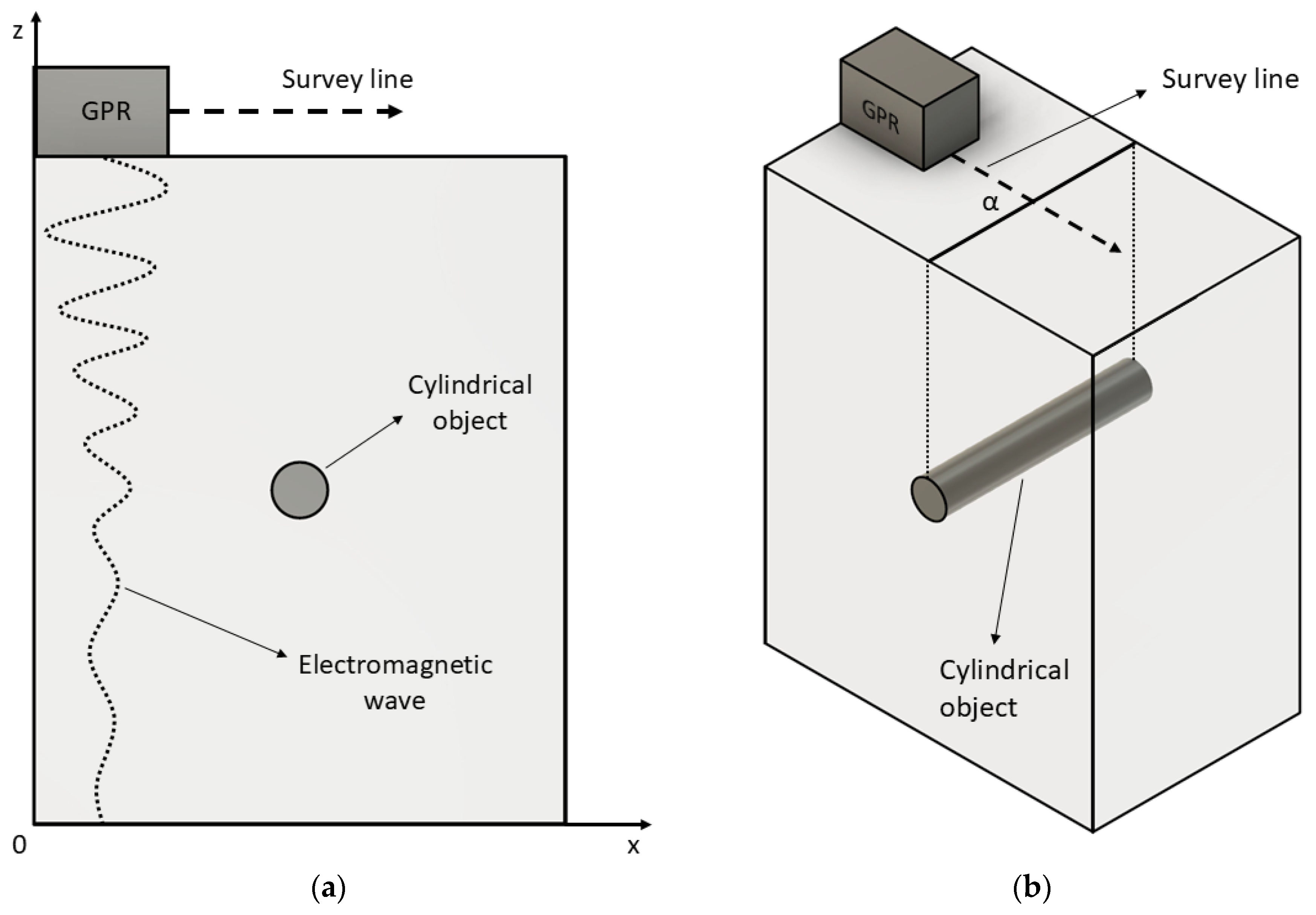Figure 2 shows the B-scan creation process utilizing a GPR in x-z coordinates, and a 3D view.

As the illustration Figure 2a shows, the x-axis represents the GPR survey line, while the z-axis is a TWTT of the EM wave, usually expressed in nanoseconds. Moreover, in a 3D view Figure 2b the parameter α represents the angle between the GPR survey line and pipeline. If the characteristics of the soil are known, then the depth of the cylindrical objects in low-loss condition can be estimated using the following equation [20]:

$$D={\displaystyle \frac{TWTTc}{2\sqrt{\epsilon \mu }}},$$

(1)

where

• TWTT—two-way travel time of EM wave,
• c—velocity of EM waves in free space (approx. 3 × 10⁸ m/s),
• ε—relative permittivity,
• μ—relative permeability.

The recordings were acquired at 33 micro-locations throughout the city of Rijeka, Croatia, resulting in a total of 1051 B-scans. At each micro-location, data were recorded in three directions: horizontal, vertical, and diagonal, in order to capture different perspectives of the subsurface features and enhance models’ robustness. Depending on the location and terrain conditions, the spacing between adjacent survey lines ranged from approximately 0.5 to 1.5 m. Data acquired in the aforementioned manner includes a range of heterogeneous and complex subsurface environments with variations in soil type, composition, and moisture content. These factors directly affect the propagation velocity of EM waves, and consequently, affect the estimation of burial depth, pipeline diameter, and angle between GPR survey line and a pipeline.

A GPR is usually characterized by small deep reflection echoes which require the use of preprocessing methods to improve signal quality and interpretability. Therefore, several standard preprocessing steps are applied to all acquired B-scans prior to model training. First, a time-zero position has to be defined. According to Yelf (2004), there are many approaches to determining time-zero, and not one correct method [21]. In the case of the GPR system utilized in this research, the experimental analysis reveals that the time-zero position is at the first break position, i.e., the first positive peak when observing the A-scan. Second, a band-pass filter was applied to attenuate both low-frequency drift and high-frequency random noise outside the effective bandwidth. Third, in order to compensate signal attenuation with depth and enhance the visibility of deeper echoes, exponential gain is utilized. These preprocessing steps are chosen to balance noise reduction and preservation of hyperbolic signatures, which are critical for reliable parameter estimation.

The positions of the pipelines were obtained from city infrastructure records, which are legally mandated to be documented with high precision under construction regulations. These records were aligned with GPR survey lines using global navigation satellite system (GNSS) with Croatian positioning system (CROPOS), which provides centimeter-level accuracy. Additional layer of quality control is employed where four independent domain experts manually refined and validated all annotations by directly inspecting the B-scans. Such annotation protocol ensures that the ground truth annotations used for training and evaluation purposes are precise and fully aligned with the object of interest. Utilizing the aforementioned approach, the angle between GPR survey line and a pipeline can be precisely calculated. This process resulted in a total of 1596 annotations. However, for 864 out of the 1596 total annotations, certain infrastructure characteristics were missing, e.g., pipeline diameter information unavailable or burial depth insufficiently precise for the purpose of this research. As a result, the remaining 732 annotations contain complete information regarding the infrastructure characteristics.

The vertical position of the top of hyperbolic reflections within the B-scans, expressed in terms of TWTT, ranged from approximately 9 to 43 nanoseconds, depending on the burial depth and the electromagnetic properties of the subsurface. The pipeline burial depths range from 0.4 to 2.0 m, while the diameters varied between 0.025 and 0.6 m. Furthermore, the angle between the GPR survey lines and a pipeline ranged from 19 to 90 degrees, encompassing a wide range of intersection geometries. For the purpose of neural network training, some of the target variables are normalized to enhance numerical stability and facilitate convergence. Specifically, the TWTT values are linearly scaled to the range between 0.0 and 1.0 for training purposes. In the case of the angle (α), the sine transformation sin(α) is employed instead of using the raw angle in degrees or radians. Pipeline burial depth and diameter are not normalized since their natural ranges are already sufficiently constrained. Such normalization stabilizes the loss computation by preventing large target value disparities and reducing the risk of gradient explosion.

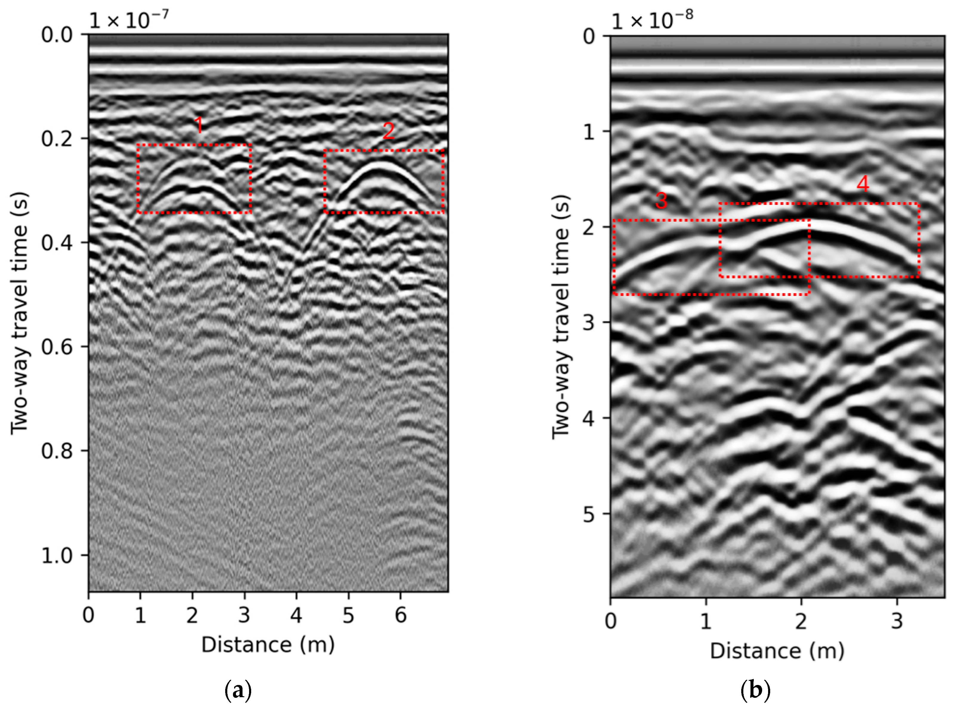
An example of two B-scans recorded using GSSI UtilityScan GPR equipped with a 350 MHz antenna at two different locations is shown in Figure 3. Moreover, the detailed characteristics of underground pipelines, which are represented by the hyperbolic reflections (1, 2, 3, 4) within the B-scans, are shown in

Table 1. Characteristics of underground pipelines in terms of TWTT, burial depth, pipeline diameter, and angle between GPR survey line and pipeline shown in Figure 3.

Hyperbolic Reflection	TWTT (ns)	Depth (m)	Diameter (m)	Angle—|α| (°)
1	22.96	0.9	0.25	87
2	24.59	1.0	0.2	87
3	20.30	1.0	0.25	38
4	18.27	0.9	0.3	43

.

All of the aforementioned parameters, i.e., vertical position in terms of TWTT and meters, diameter, and angle, affect the shape of the resulting hyperbolic reflections within the B-scan, thereby increasing complexity and interpretation. For that reason, this research proposes a simultaneous estimation of these parameters, enabling more robust and accurate characterization of underground infrastructure.

2.2. Detection and Localization of Cylndrical Objects

Underground pipelines, when surveyed using GPR, appear as hyperbola-shaped features within the B-scan profiles. Since these features represent the primary objects of interest in this research, two state-of-the-art AI object detection algorithms are employed for their identification and localization, namely, you only look once (YOLO) version 11 and real-time detection transformer (RT-DETR).

2.2.1. You Only Look Once v11

The first algorithm utilized is YOLOv11 representing the most recent iteration of the YOLO series of object detection models. YOLOv11 introduces substantial improvements in both architecture and training methodology, making it a versatile and efficient choice for various computer vision tasks. Key enhancements include improved feature extraction, optimization for speed and computational efficiency, and increased accuracy despite a reduction in model size [22]. Interestingly, the YOLOv11m model resulted in higher mean average precision (mAP) on the COCO dataset while using 22% fewer parameters than YOLOv8m.

Key innovations include the integration of the cross stage partial with kernel size 2 (C3k2) block, spatial pyramid pooling-fast (SPFF), and convolutional block with parallel spatial attention (C2PSA) components. These architectural elements contribute to more effective feature extraction and processing, enabling the model to better analyze and interpret complex visual information [23]. The C2PSA component, in particular, represents a significant advancement in spatial attention mechanisms, allowing the model to focus more effectively on critical regions within the image and enhancing its capability to detect and analyze partially occluded or complex objects [22]. YOLOv11 introduces a range of model variants, from nano to extra-large configurations. This scalability enables deployment across various environments. Beyond traditional object detection, YOLOv11 demonstrates multi-task proficiency including image classification, instance segmentation, pose estimation, and oriented object detection. Therefore, YOLOv11 as a unified framework is capable of addressing multiple computer vision challenges within a single architectural paradigm.

2.2.2. Real-Time Detection Transformer

RT-DETR represent a paradigm shift in object detection methodology, introducing a real-time end-to-end transformer-based framework that effectively addresses the computational limitations traditionally associated with DETR-based architectures. While the original DETR architecture eliminates the need for hand-crafted anchor and non-maximum suppression (NMS) components by employing bipartite matching to directly produce one-to-one set predictions, on the other hand, it suffers from slow training convergence, high computational cost, and hard-to-optimize queries [24]. Therefore, many DETR variants have been proposed to overcome the aforementioned limitations.

The development of RT-DETR follows a two-step process: initially focusing on maintaining detection accuracy while improving processing speed, followed by maintaining speed while improving accuracy [25]. The architecture itself consists of three primary components: a convolutional backbone network, a hybrid encoder, and a transformer decoder with auxiliary prediction heads. Among the key innovations in RT-DETR are the hybrid encoder and the uncertainty-minimal query selection. The hybrid encoder is designed to expeditiously process multi-scale features by decoupling intra-scale interactions and cross-scale fusion operations. Such architectural separation enables efficient feature processing while maintaining the model’s ability to capture both local and global contextual information. The uncertainty-minimal query selection, recognized as a critical advancement, improves the quality of the initial object queries provided to the decoder [26]. The transformer decoder, which is equipped with auxiliary prediction heads, iteratively optimizes object queries to output classification labels and bounding box coordinates. Furthermore, RT-DERT supports flexible speed-accuracy trade-offs by allowing the adjustment of decoder layers, enabling adaptation to diverse computational constraints and deployment scenarios.

2.3. Estimation of Underground Infrastructure Characteristics

After the detection and localization of hyperbolic reflections within the B-scans utilizing the object detection algorithms described in the previous subsection, the estimation of underground infrastructure characteristics is performed. The output of the detection algorithm, in the form of bounding box coordinates, is used to crop the corresponding regions of the B-scan, which are then employed for estimating the characteristics of the underground infrastructure. More specifically, the B-scan is cropped according to the bounding box dimensions provided by the object detection step. For each detected hyperbolic reflection, the relevant segment is extracted from the original B-scan based on the estimated bounding box coordinates. Importantly, the absolute position along the vertical axis is preserved during cropping, as this parameter critically influences the geometry and shape of the hyperbolic reflection. In this manner, the extracted hyperbolic features retain both the spatial and structural information necessary for accurate parameter estimation.

In order to simultaneously estimate the parameters of underground infrastructure (TWTT, burial depth, pipeline diameter, and the angle between GPR survey line and a pipeline), adapted deep learning model architectures are employed.

An overview of deep learning model architectures is given as follows:

• DenseNet—Huang et al. (2016) introduced the dense convolutional network (DenseNet), which has several advantages, including alleviating the vanishing-gradient problem, strengthening feature propagation, encouraging feature reuse, and reducing the number of parameters [27]. The aforementioned is possible due to the dense connectivity among layers, where each layer receives direct input from all preceding layers and passes its own feature maps to all subsequent layers in a feed-forward manner. The dense connectivity facilitates direct access to gradients from the loss function and original signal throughout the neural network hierarchy, thereby improving training stability and convergence properties [28]. Due to the high efficiency and robustness to overfitting on small datasets, the architecture is widely adopted across various application domains in computer vision.
• Xception—The architecture proposed by Chollet (2017) represents a significant advancement in depthwise separable convolutions through the reformulation of the Inception hypothesis [29]. Innovation employs depthwise separable convolutions as the fundamental building block, where Inception modules are replaced by depthwise convolutions followed by pointwise convolutions. The underlying hypothesis posits that cross-channel and spatial correlations in feature maps can be entirely decoupled. The depthwise separable convolution mechanism enables parameter reduction, lower computational cost, and enhanced model efficiency while at the same time maintaining comparable or superior performance [30]. According to the aforementioned, the Xception model architecture is particularly suitable for applications and environments where an optimal balance between model complexity and performance is required.
• NASNet—Leveraging neural architecture search (NAS) techniques, Zoph et al. (2018) introduced a method to automatically design the model architectures directly on the dataset of interest [31]. In order to discover optimal convolutional cell structures, the reinforcement learning-based search algorithms are utilized. This way the traditional architectures are replaced by algorithmically optimized building blocks. The automated search mechanism systematically explores architectural configurations, optimizing both computational efficiency and performance [32]. The search process identifies transferable convolutional cells that can be stacked to construct neural networks of varying depths. Consequently, the NASNet model architecture is suitable for applications where state-of-the-art performances are required.
• EfficientNetV2—By combining training-aware neural architecture search and scaling, Tan and Le (2021) developed a family of EfficientNetV2 models that have better parameter efficiency and faster training speed [33]. According to the authors, the training efficiency can be improved by incorporating Fused-MBConv blocks alongside traditional MBConv blocks and implementing progressive resizing during training. In order to allow the model to learn from smaller, less regularized images before progressing to full resolution inputs, the progressive learning mechanism is utilized which gradually increases image resolution and regularization strength during training [34]. Therefore, EfficientNetV2 is suited for applications where fast model deployment and high training efficiency are crucial.
• ConvNeXt—In their work, Liu et al. (2022) modernize the traditional ConvNet architectures utilizing vision transformer design principles [35]. The innovation utilizes comprehensive redesign approach where standard ResNet components are modernized through the incorporation of large kernel convolutions, inverted bottleneck structures, and advanced normalization techniques. The authors stated that pure convolutional networks can achieve competitive performance with vision transformers by adopting their architectural innovations while maintaining the advantages of convolutions. As a result, ConvNeXt family models are outperforming Swin Transformers in terms of performance and scalability while maintaining the simplicity and efficiency of standard ConvNets [36]. Therefore, such architecture is utilized in applications where performance levels of state-of-the-art vision transformers and computational efficiency of traditional ConvNets are required.

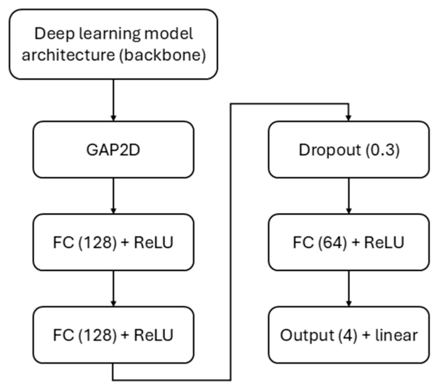
All deep learning model architectures employed in this research utilized ImageNet pretrained backbones as feature extractors. In order to adapt the aforementioned models for multi-variable regression, a custom model head is implemented with the following architecture: A global average pooling 2D (GAP2D) layer is applied to the backbone features, followed by two sequential fully connected (FC) layers, each containing 128 neurons with ReLU activation functions. Subsequently, dropout regularization with a rate of 0.3 is applied in order to prevent overfitting, followed by an additional FC layer consisting of 64 neurons with ReLU activation function. The final output layer consists of four neurons and a linear activation function in order to enable simultaneous regression of four target variables. The custom model head is shown in Figure 4.

2.4. Evaluation Criteria

For the purpose of evaluating the performance of the deep learning models utilized in this research, several performance measures are employed. For object detection purposes precision, recall, and mean average precision (mAP) are utilized. The mAP calculation relies on the precision, recall, and intersection over union (IoU), which can be mathematically described as follows [37]:

$$Precision={\displaystyle \frac{TP}{TP+FP}},$$

(2)

$$Recall={\displaystyle \frac{TP}{TP+FN}},$$

(3)

and

$$IoU={\displaystyle \frac{\left|A\cap B\right|}{\left|A\cup B\right|}},$$

(4)

where

• TP—true positive,
• FP—false positive,
• FN—false negative,
• $A\cap B$—the area where the estimated and ground truth boxes overlap, and
• $A\cup B$—the total area covered by both bounding boxes.

The mAP is calculated through a multi-step process which involves calculating precision and recall at various IoU thresholds, followed by calculating the AP for each threshold, and afterwards averaging the AP values to obtain the mAP score. The performance measures defined by Equations (2)–(4) have a value range between 0.0 and 1.0, with higher values indicating better model performance.

In the case of parameter estimation, which is a regression problem, the coefficient of determination—R², mean absolute error (MAE), and root mean squared error (RMSE) are employed, which can be mathematically represented as [38]:

$$R^2=1-{\displaystyle \frac{{SS}_{res}}{{SS}_{tot}}}={\displaystyle \frac{{\sum }_i{\left(y_i-{\hat{y}}_i\right)}^2}{{\sum }_i{\left(y_i-\overline{y}\right)}^2}},$$

(5)

$$MAE={\displaystyle \frac{1}{n}}\sum _{i=1}^n\left|y_i-{\hat{y}}_i\right|,$$

(6)

and

$$RMSE=\sqrt{{\displaystyle \frac{1}{n}}\sum _{i=1}^n{\left(y_i-{\hat{y}}_i\right)}^2}.$$

(7)

with $y_i$ being true value and ${\hat{y}}_i$ being estimated value while $\overline{y}$ represents the mean of all observed true values. The $R^2$ ranges from 0.0 to 1.0, where a value of 0.0 indicates that the model explains none of the variability in the dependent variable, while a value of 1.0 indicates that the model explains all the variability in the data. Furthermore, the lower values of measures defined by Equations (6) and (7) correspond to better performances of the model.

Additionally, k-fold cross-validation is utilized in order to perform a reliable estimation of models’ performances. Such a method represents a robust resampling technique widely used in machine learning to evaluate model performance and mitigate overfitting by ensuring reliable generalization to unseen data [39]. The dataset is divided into “k” equally sized folds, and the model is trained and evaluated k times, each time using a different fold as the validation set while the remaining k-1 folds are used for training [40]. The resulting performance measures from each fold are then averaged to provide a comprehensive and unbiased estimate of the model’s effectiveness. Such an approach ensures that all samples from the dataset contribute to both the training and validation processes.

3. Results and Discussion

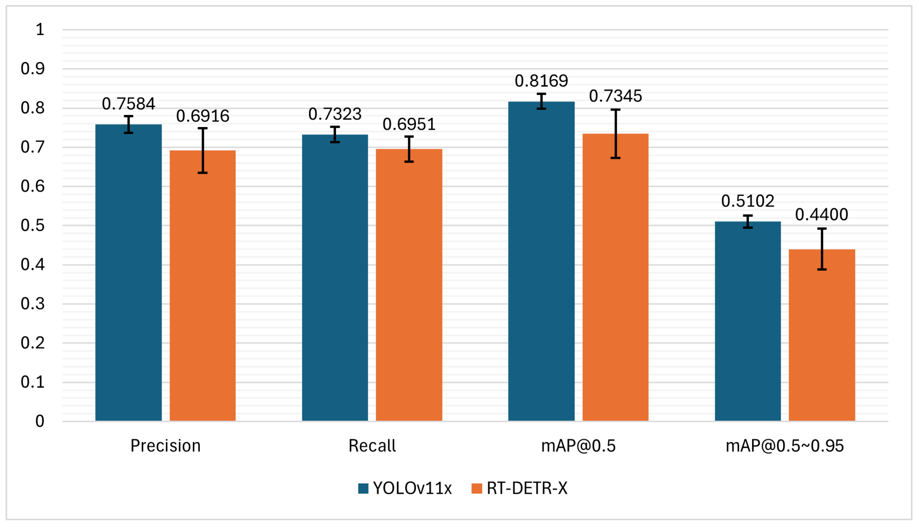
In this section, the experimental results of the proposed methodology are shown. In the first step of the proposed automated system, YOLOv11x and RT-DETR-X are trained in order to perform detection and localization of hyperbolic reflection from GPR B-scans. In both model families, the “x” variant represents the largest and best performing model architecture. These variants are utilized in applications where the performance is crucial, at the cost of computational requirements. As for the training process of YOLOv11x and RT-DETR-X models, an AdamW optimization algorithm is utilized with the initial learning rate of 0.01, final learning rate factor of 0.01, momentum of 0.937, and weight decay of 0.0005. The training is performed for 300 epochs with early stopping enabled in order to prevent overfitting. A batch size of 16 is utilized in both cases; however, an input image resolution of 640 × 640 is used for the YOLOv11x, and 720 × 720 for the RT-DETR-X. Additionally, for the object detection task only, the data augmentation is performed, which includes mosaic, horizontal flipping, translation, scaling, and random erasing in order to enhance models’ generalization. Performances of the aforementioned object detection models are evaluated utilizing 5-fold cross-validation to ensure a stable estimate and generalization. The comparative evaluation of YOLOv11x and RT-DETR-X models in detecting and localizing hyperbolic reflections within the B-scans is shown in Figure 5.

From the results, it can be seen that YOLOv11x consistently outperforms RT-DETR-X across all measured performance metrics, exhibiting both higher performance and greater stability. YOLOv11x achieved precision of 0.7584 ± 0.0213 and recall of 0.7323 ± 0.0195 across 5-folds, thereby outperforming RT-DETR-X, which has resulted in 0.6916 ± 0.0569 precision and 0.6951 ± 0.0320 recall. Analyzing these results, it can be concluded that YOLOv11x identifies a larger proportion of true positives and, at the same time, produces fewer false positives. Furthermore, in the task of detecting and localizing hyperbolic reflections from the B-scans, the superiority of YOLOv11x is reflected in its mAP@0.5 of 0.8169 ± 0.0190 and mAP@0.5~0.95 of 0.5102 ± 0.0153, surpassing RT-DETR-X, which resulted in 0.7345 ± 0.0616 and 0.4400 ± 0.0523, respectively. Additionally, the smaller values of standard deviations observed for YOLOv11x across 5-folds suggest more stable and reliable detection performance. On the other hand, RT-DETR-X demonstrates greater variability, particularly in mAP measures. Although competitive, RT-DETR-X, which uses transformer-based architecture, may require larger datasets or further fine-tuning to achieve comparable consistency and performance.

The second step of the proposed automated system is dedicated to estimating characteristic parameters of underground infrastructure situated within heterogeneous and complex soil environments, including TWTT of the object, burial depth, pipeline diameter, and angle between GPR survey line and pipeline. The output from the first step, i.e., detected and localized hyperbolic reflections are used as input data to the second step of the system. The parameter estimation framework employs state-of-the-art deep learning model architectures, leveraging pretrained models as feature extraction backbones. The implemented model architectures comprise DenseNet201, Xception, NASNetLarge, EfficientNetV2L, and ConvNeXtLarge, where each is utilized as a feature extraction component. The aforementioned backbones, which are pretrained on ImageNet, are adapted by adding a custom designed regression head architecture, which is provided in Figure 4. The model training procedure for estimating characteristic parameters of underground infrastructure is designed to achieve robust regression performance through an adaptive learning strategy and a custom weighted mean squared error (MSE) loss function. The model is trained for 500 epochs with an initial learning rate of 0.0001 and a batch size of 4, optimized using the Adam optimization algorithm. The custom loss function is implemented as a weighted MSE, where the estimations from the output layer are scaled by predefined importance weights with the values of 1.0, 1.0, 1.5, and 3.0 for the TWTT, burial depth, diameter, and angle, respectively. Such an approach facilitates the prioritization of learning for more complex and critical output parameters, thereby enhancing the overall estimation performance and robustness of the models in question. By assigning higher weights to outputs of greater difficulty, the training process guides the network to allocate more representational capacity toward challenging estimations. In order to ensure efficient model convergence and prevent overfitting, the training process incorporates adaptive learning rate reduction and early stopping mechanisms. More precisely, the learning rate is progressively decreasing during the periods of loss stagnation, i.e., the learning rate is reduced by a factor of 0.8 after 20 epochs of non-improvement. Since the TWTT values are normalized to the range between 0.0 and 1.0 for training purposes, these values are denormalized to their original scale during the performance evaluation in order to ensure that error values obtained from MAE and RMSE are expressed in the same physical units as the original TWTT measurements.

Performances of the aforementioned model architectures in estimating characteristic parameters of underground infrastructure, i.e., TWTT, burial depth, pipeline diameter, and angle between GPR survey line and pipeline, are shown in

Table 2. Performances of DenseNet201, Xception, NASNetLarge, EfficientNetV2L, and ConvNeXtLarge model architectures in TWTT estimation from hyperbolic reflection in B-scan data. Performance measures are expressed as mean ± standard deviation from 5-fold cross-validation.

Backbone	R2 ± σ	MAE ± σ	RMSE ± σ
DenseNet201	0.9490 ± 0.0182	1.1223 ± 0.1998	1.4286 ± 0.2389
Xception	0.9702 ± 0.0056	0.8508 ± 0.1012	1.1053 ± 0.1162
NASNetLarge	0.9630 ± 0.0137	0.9053 ± 0.1193	1.2174 ± 0.2077
EfficientNetV2L	0.9716 ± 0.0043	0.8224 ± 0.0625	1.0798 ± 0.0713
ConvNeXtLarge	0.8649 ± 0.0829	1.8537 ± 0.6909	2.2579 ± 0.7077

,

Table 3. Performances of DenseNet201, Xception, NASNetLarge, EfficientNetV2L, and ConvNeXtLarge model architectures in burial depth estimation from hyperbolic reflection in B-scan data. Performance measures are expressed as mean ± standard deviation from 5-fold cross-validation.

Backbone	R2 ± σ	MAE ± σ	RMSE ± σ
DenseNet201	0.9464 ± 0.0171	0.0504 ± 0.0079	0.0685 ± 0.0100
Xception	0.9587 ± 0.0056	0.0436 ± 0.0023	0.0608 ± 0.0049
NASNetLarge	0.9482 ± 0.0110	0.0498 ± 0.0068	0.0677 ± 0.0074
EfficientNetV2L	0.9631 ± 0.0050	0.0413 ± 0.0022	0.0574 ± 0.0045
ConvNeXtLarge	0.9232 ± 0.0222	0.0621 ± 0.0116	0.0821 ± 0.0113

,

Table 4. Performances of DenseNet201, Xception, NASNetLarge, EfficientNetV2L, and ConvNeXtLarge model architectures in pipeline diameter estimation from hyperbolic reflection in B-scan data. Performance measures are expressed as mean ± standard deviation from 5-fold cross-validation.

Backbone	R2 ± σ	MAE ± σ	RMSE ± σ
DenseNet201	0.5532 ± 0.1034	0.0378 ± 0.0060	0.0536 ± 0.0026
Xception	0.6579 ± 0.0136	0.0312 ± 0.0008	0.0475 ± 0.0033
NASNetLarge	0.5887 ± 0.0470	0.0350 ± 0.0028	0.0520 ± 0.0043
EfficientNetV2L	0.6822 ± 0.0381	0.0312 ± 0.0015	0.0458 ± 0.0045
ConvNeXtLarge	0.4575 ± 0.1500	0.0452 ± 0.0085	0.0594 ± 0.0095

and

Table 5. Performances of DenseNet201, Xception, NASNetLarge, EfficientNetV2L, and ConvNeXtLarge model architectures in α (angle between GPR survey line and pipeline) estimation from hyperbolic reflection in B-scan data. Performance measures are expressed as mean ± standard deviation from 5-fold cross-validation.

Backbone	R2 ± σ	MAE ± σ	RMSE ± σ
DenseNet201	0.6048 ± 0.0271	0.0676 ± 0.0060	0.0849 ± 0.0051
Xception	0.7335 ± 0.0548	0.0483 ± 0.0098	0.0697 ± 0.0098
NASNetLarge	0.6633 ± 0.0987	0.0544 ± 0.0069	0.0778 ± 0.0126
EfficientNetV2L	0.7544 ± 0.0669	0.0428 ± 0.0071	0.0667 ± 0.0115
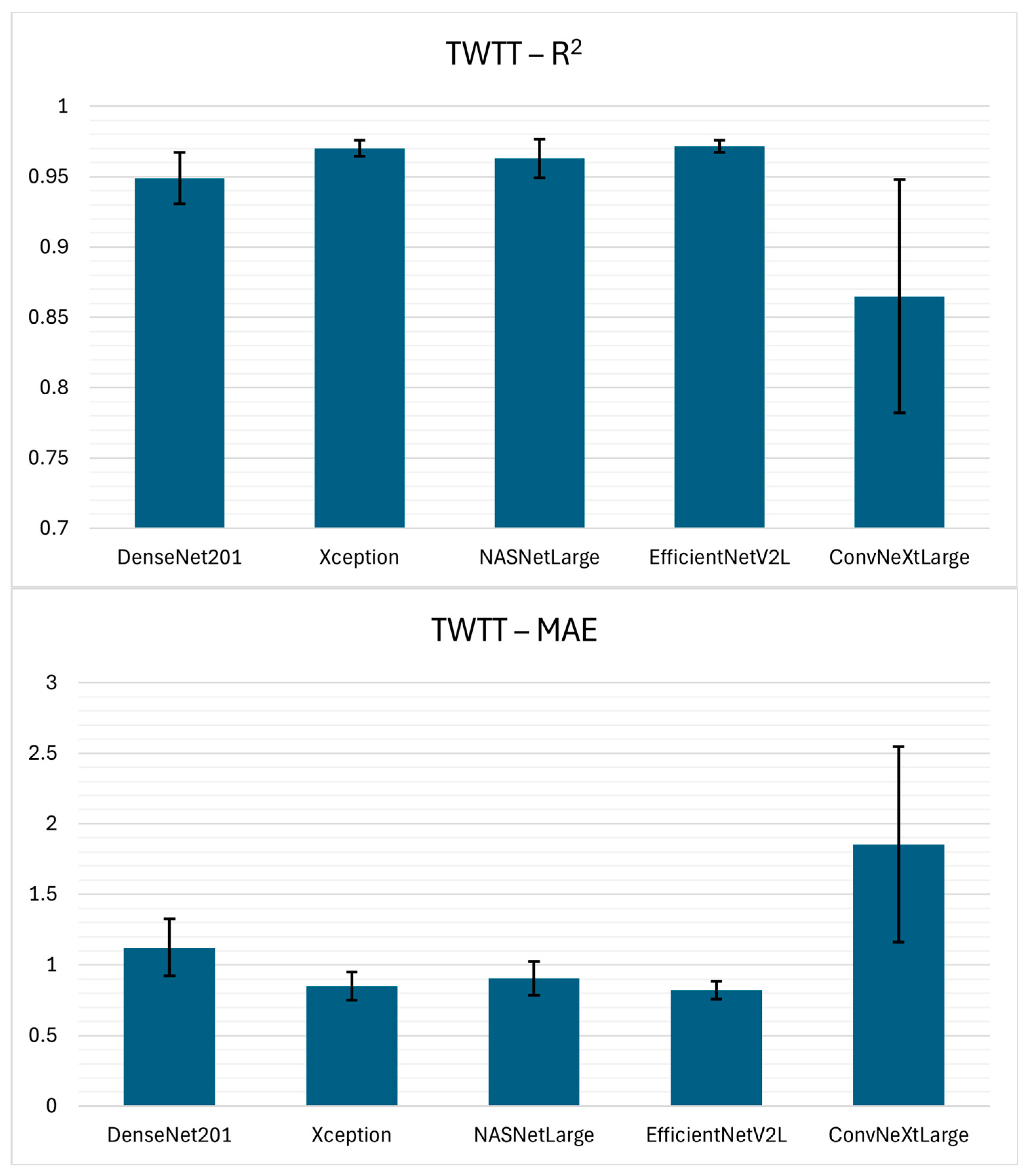
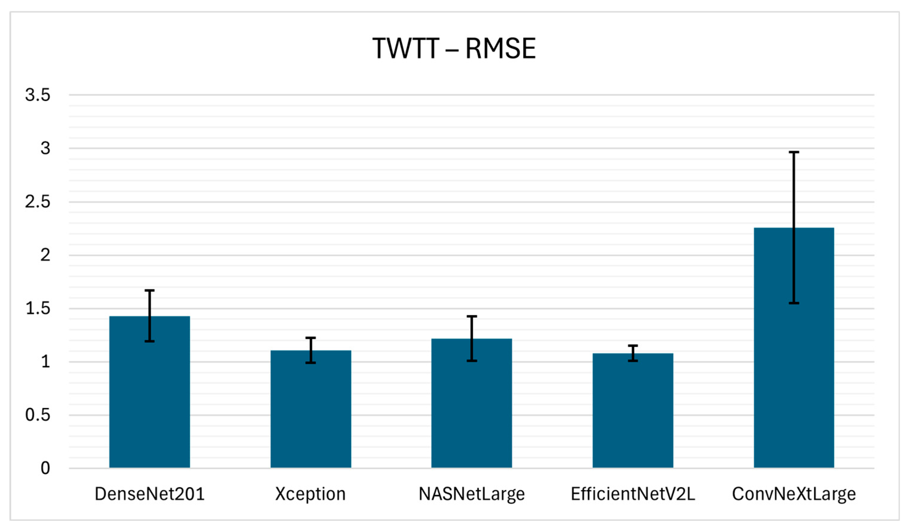
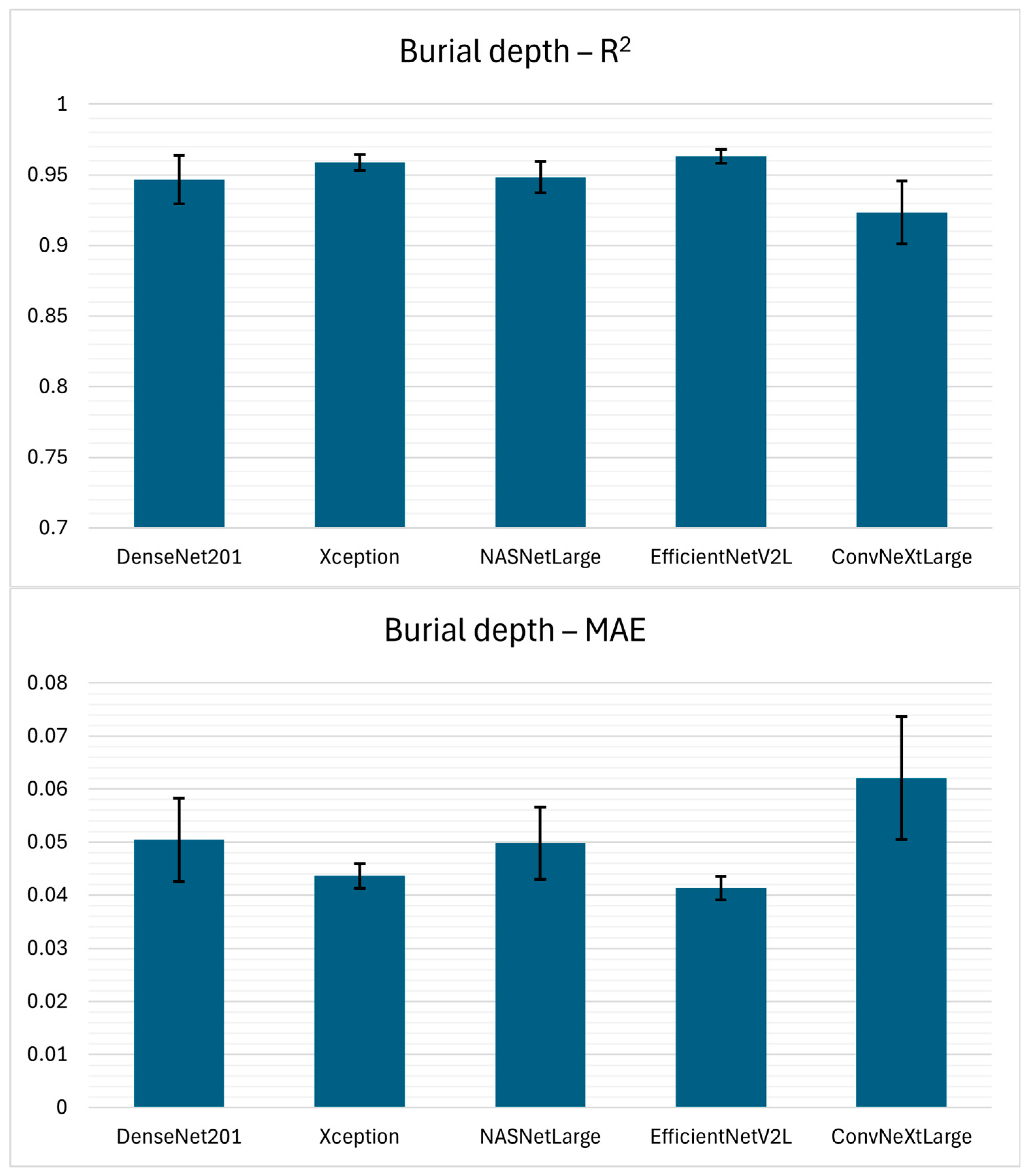
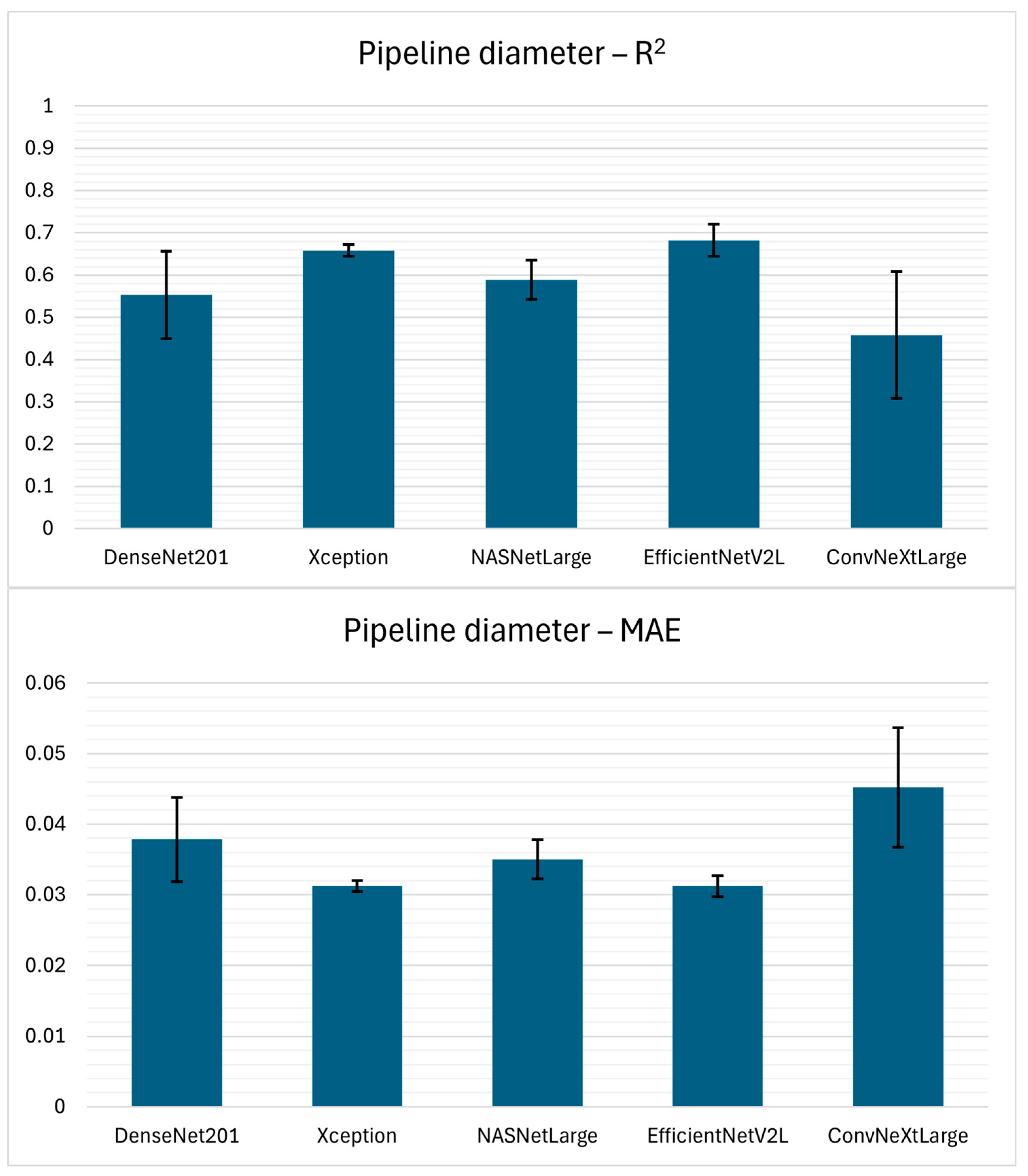
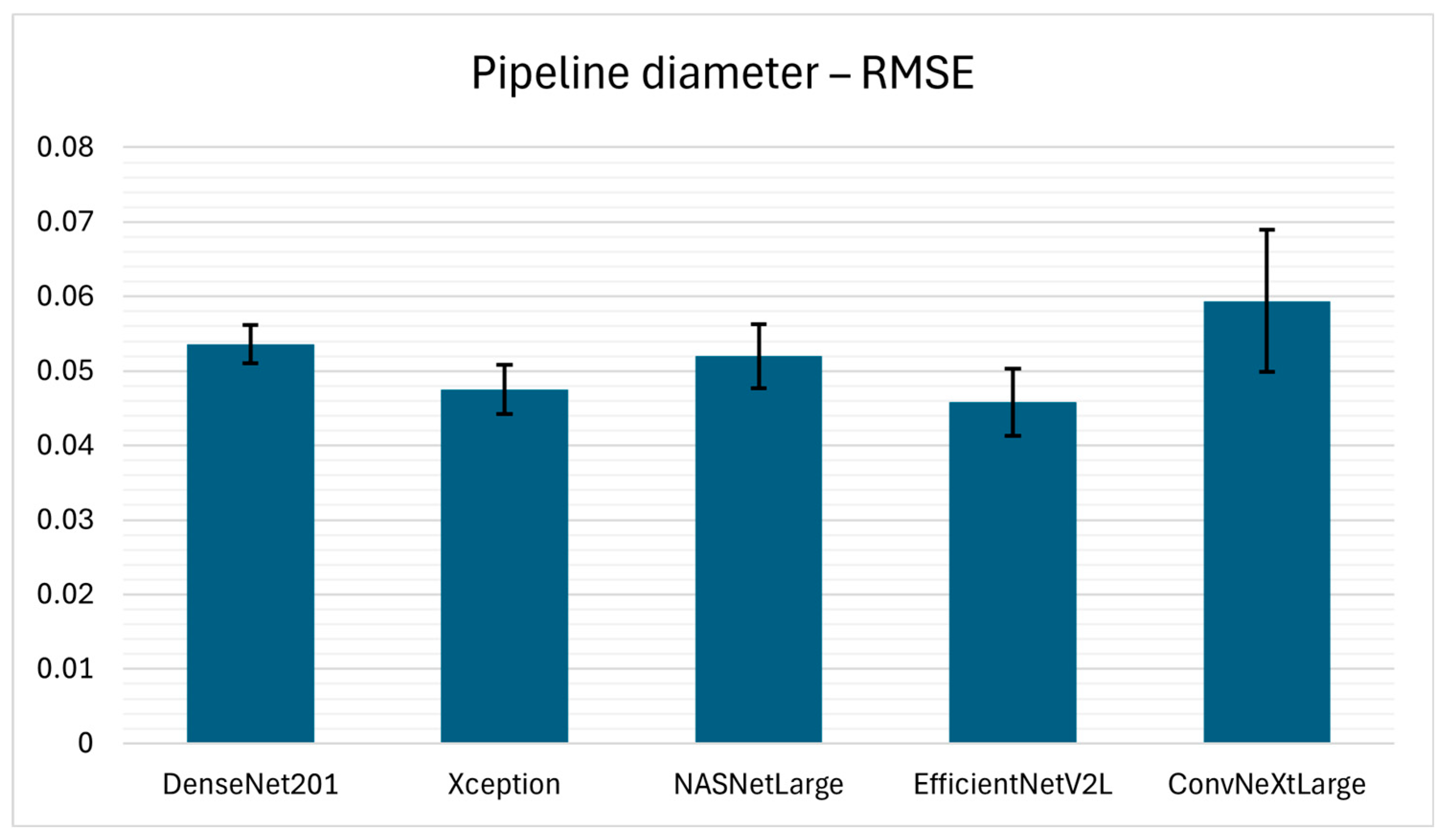
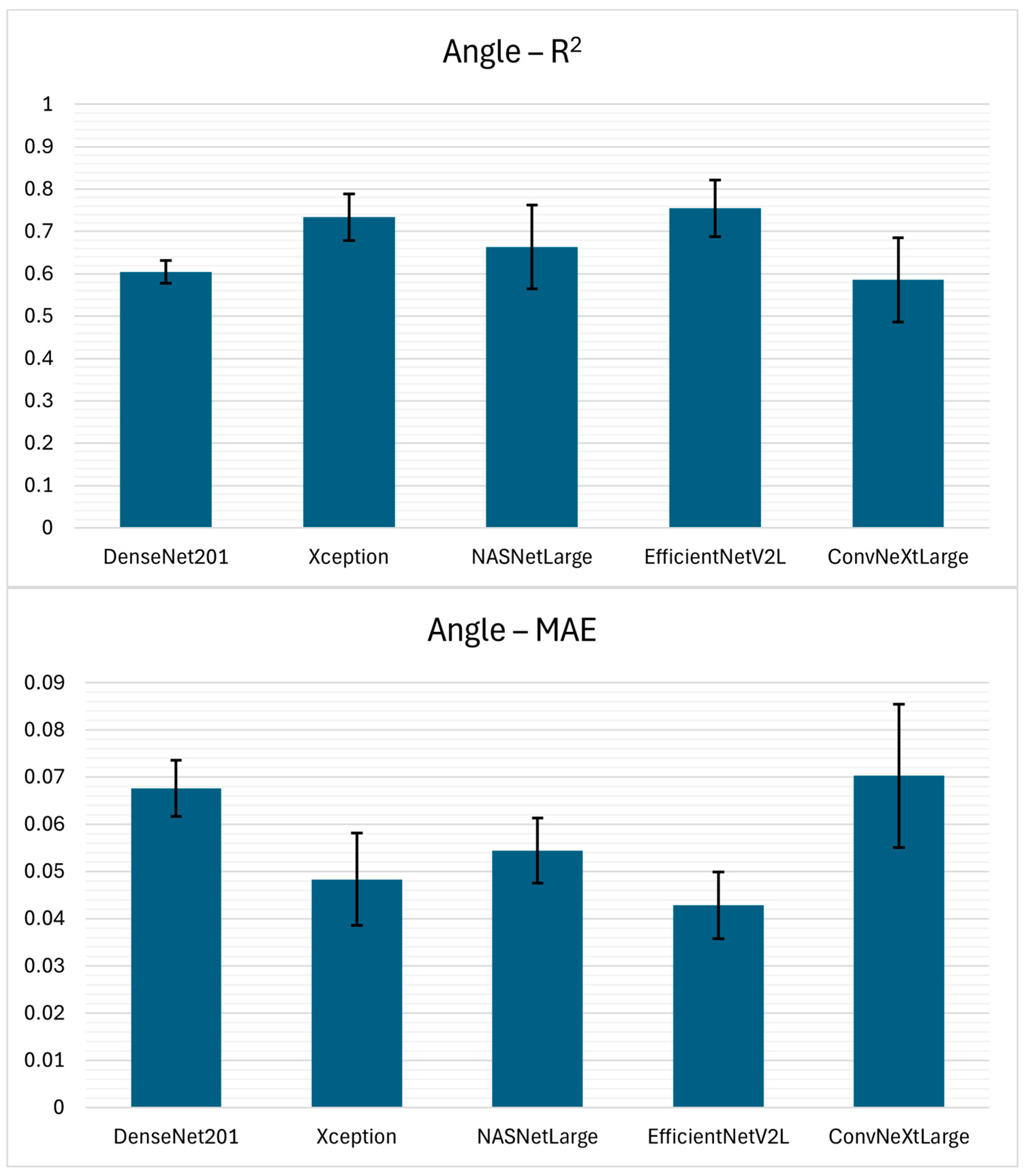
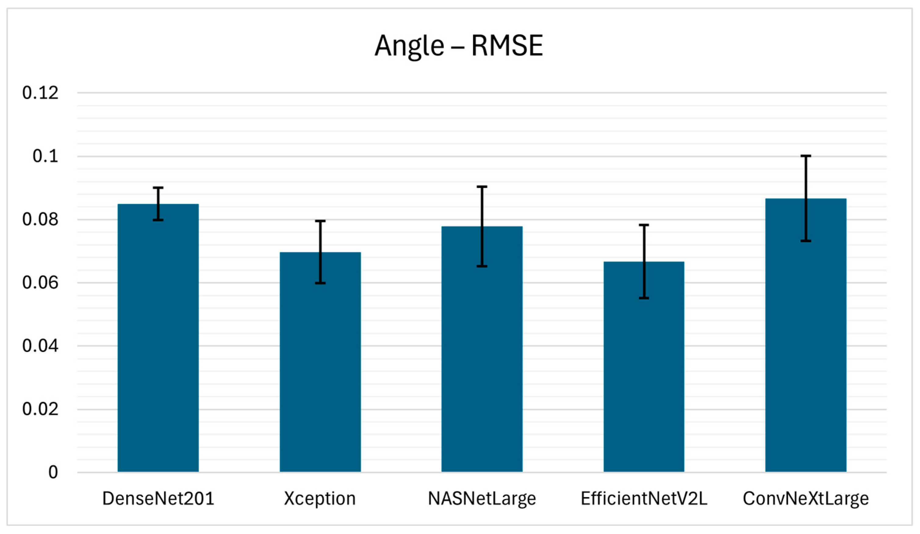
ConvNeXtLarge	0.5855 ± 0.0990	0.0703 ± 0.0152	0.0867 ± 0.0134

. Additionally, graphical representations of the performances are provided in Appendix A (Figure A1, Figure A2, Figure A3 and Figure A4).

According to the results for TWTT estimation from hyperbolic reflection, EfficientNetV2L achieved the highest performance, with an R² of 0.9716 ± 0.0043, a MAE of 0.8224 ± 0.0625, and an RMSE of 1.0798 ± 0.0713, indicating superior performance and stability across the 5-fold cross-validation. Xception yielded comparable performance, with an R² of 0.9702 ± 0.0056 and slightly higher errors (MAE 0.8508 ± 0.1012, RMSE 1.1053 ± 0.1162). NASNetLarge followed closely with an R² of 0.9630 ± 0.0137, however the error performance measures (MAE 0.9053 ± 0.1193, RMSE 1.2174 ± 0.2077) indicate less precise estimations compared to EfficientNetV2L and Xception.

The evaluation of burial depth estimation performance is performed across five deep learning model architectures. From the performance evaluation it can be seen that EfficientNetV2L achieved the highest performance, resulting in R² of 0.9631 ± 0.0050, MAE of 0.0413 ± 0.0022, and RMSE of 0.0574 ± 0.0045, reflecting low variability across 5-fold cross-validation. Moreover, the Xception model architecture achieved the second-best results, achieving an R² of 0.9587 ± 0.0056, MAE of 0.0436 ± 0.0023, and RMSE of 0.0608 ± 0.0049. NASNetLarge also performed competitively, achieving an R² of 0.9482 ± 0.0110; however, at the same time, the error measures (MAE 0.0498 ± 0.0068, RMSE 0.0677 ± 0.0074) suggest lower precision compared to EfficientNetV2L and Xception.

The experimental results for pipeline diameter estimation from hyperbolic reflections in GPR B-scan data indicate that such a regression task is considerably more challenging than TWTT and burial depth estimation, as reflected by the lower values of performance measures given in Table 4. Among the evaluated model architectures, EfficientNetV2L yielded the highest estimation performance with the values of 0.6822 ± 0.0381, 0.0312 ± 0.0015, and 0.0458 ± 0.0045, for R², MAE, and RMSE, respectively. Again, Xception demonstrated comparable performance, reaching an R² of 0.6579 ± 0.0136, MAE of 0.0312 ± 0.0008, and RMSE of 0.0475 ± 0.0033. The standard deviation values show low variability, indicating strong consistency across 5-folds. NASNetLarge and DenseNet201 produced moderate results, while ConvNeXtLarge underperformed substantially.

In the case of the α estimation, EfficientNetV2L again achieved superior results compared to other model architectures with the values of 0.7544 ± 0.0669, 0.0428 ± 0.0071, and 0.0667 ± 0.0115 for R², MAE, and RMSE, respectively. These results are followed closely by the Xception model architecture, achieving an R² of 0.7335 ± 0.0548, MAE of 0.0483 ± 0.0098, and RMSE of 0.0697 ± 0.0098. Furthermore, NASNetLarge demonstrated intermediate performance, while DenseNet201 and ConvNeXtLarge achieved the lowest performance.

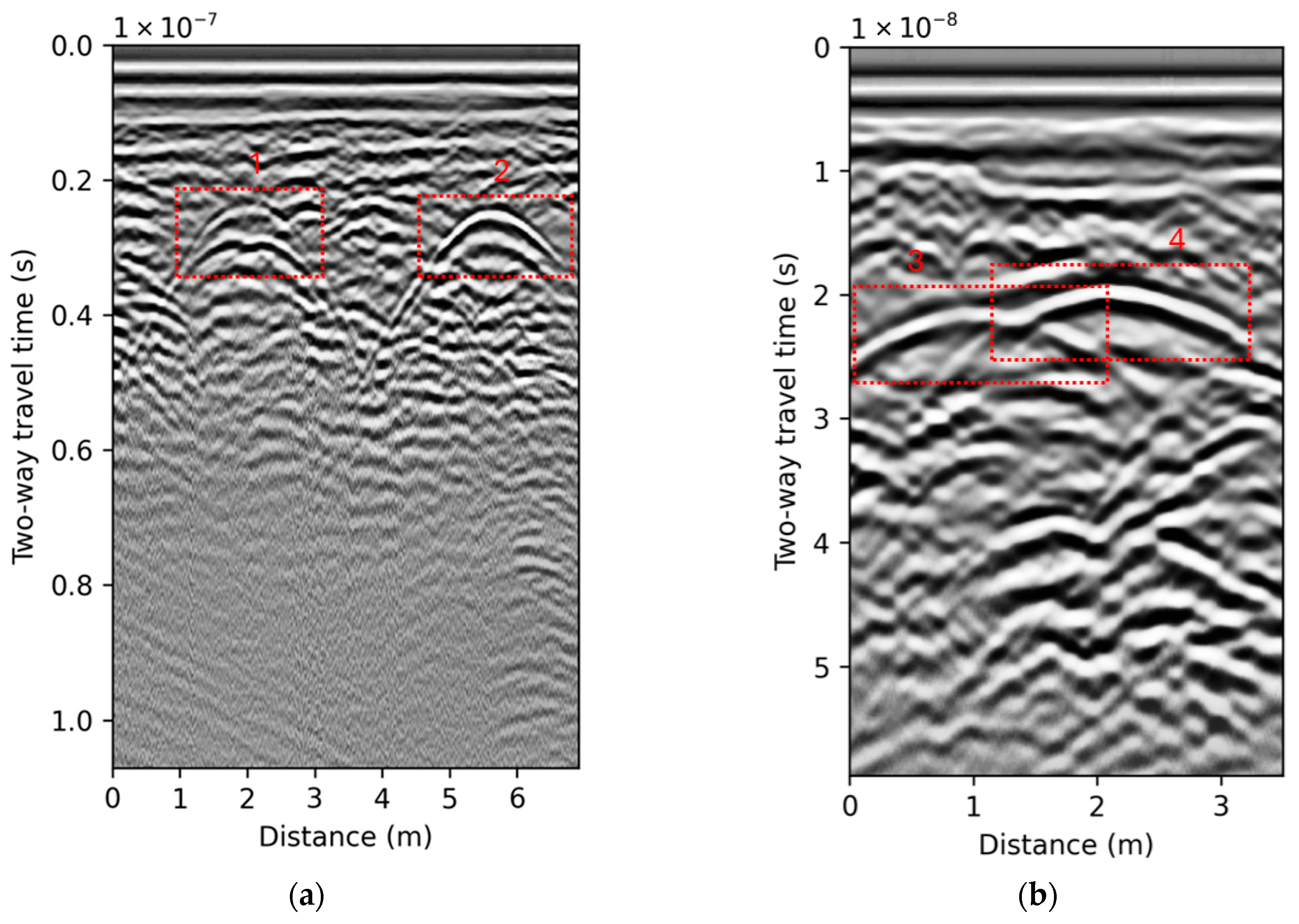
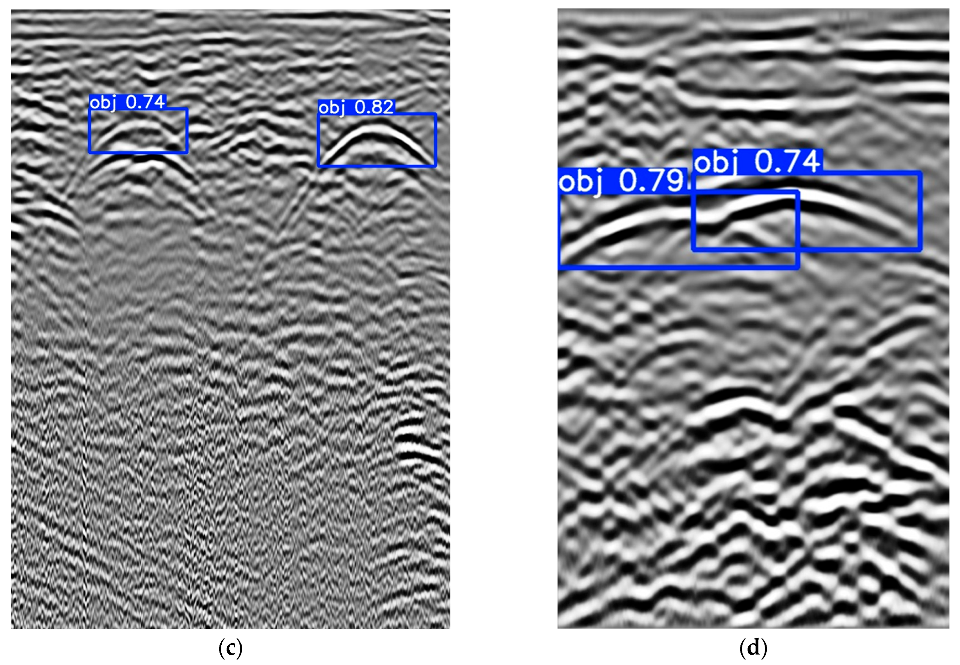
Figure 6 presents the output of the detection step of the proposed automated system, visualized on a representative subset of B-scan data. The figure highlights the localization of hyperbolic reflections corresponding to underground infrastructure. Subsequently,

Table 6. True and estimated parameters of underground pipelines in terms of TWTT, burial depth, pipeline diameter, and angle between GPR survey line and pipeline shown in Figure 6.

Hyperbolic Reflection	TWTT (ns)		Depth (m)		Diameter (m)		Angle—|α| (°)
	True	Est.	True	Est.	True	Est.	True	Est.
1	22.96	22.68	0.9	1.0	0.25	0.18	87	83
2	24.59	22.36	1.0	0.98	0.2	0.2	87	83
3	20.30	21.27	1.0	0.97	0.25	0.2	38	41
4	18.27	17.89	0.9	0.82	0.3	0.22	43	46

provides a comparison of true and the model estimated characteristics parameters, thereby quantitatively illustrating the system’s estimation performance.

It is important to emphasize that the dataset used includes real-world GPR data acquired at multiple locations, where non-pipeline hyperbolic reflections (e.g., stones, reflections from other pipelines or other underground features) are also present. Such examples can even be observed in Figure 6 between boxes 1 and 2 in Figure 6a, and above and below box 3 in Figure 6b. The detection algorithm did not label these features as pipelines, which confirms that the model is trained specifically to detect pipeline-related hyperbolic reflections while discarding others. Such detection of false positives will also have an impact which will result in decreased values of performance measures. Moreover, the proposed two-step framework further reduces the impact of this issue. In the second step, parameter estimation of the detected hyperbolic reflection is performed. If the estimated parameters fall outside the expected range for pipelines, the reflection can be discarded.

Considering the results of the proposed automated system dedicated to estimating characteristic parameters of underground infrastructure situated within heterogeneous and complex soil environments, it can be observed that TWTT and burial depth estimations are the highest performing. The R² values exceeded 0.94 for all model architectures, making it a less complex regression problem compared to the estimation of pipeline diameter, and angle between GPR survey line and pipeline. The TWTT is a directly observable parameter in B-scan data with mostly clear visual cues (apex of the hyperbola), allowing CNN-based feature extractors to achieve high regression performance. Nevertheless, precise localization of the hyperbola apex remains critical, regardless of whether the reflection is produced by metallic, plastic, or concrete pipelines. Therefore, with the assistance of DL models, a TWTT parameter can be estimated with greater robustness, and efficiency.

Similar to TWTT, burial depth estimation yielded high regression performance with R² values ranging between 0.92 and 0.96. The reason for such results is the fact that burial depth is closely related to TWTT which is also mathematically described with an Equation (1). However, burial depth cannot be directly determined until the EM wave velocity within the soil is either estimated or directly measured. Consequently, precise interpretation of hyperbolic signatures is of critical importance, since the velocity information required for burial depth estimation is inherently encoded in the geometry of the hyperbolic response. The proposed approach shows that such information can be effectively extracted and analyzed, thereby enabling reliable burial depth estimation.

In contrast, pipeline diameter and angle estimation are considered as high complexity regression problems which can be seen from the presented results where R² values range from 0.45 to 0.75. Pipeline diameter estimation is particularly challenging since hyperbolic width is subtle and often distorted by soil heterogeneity, noise, and partial reflections. Unlike TWTT and burial depth, diameter is not explicitly encoded in a single visual feature but requires contextual interpretation of the hyperbola curvature, which explains the reduced R² values. Angle between GPR survey line and pipeline is indirectly encoded in the asymmetry and elongation of hyperbolic reflections, which are also often subtle and affected by noise or incomplete reflections. This explains both the lower R² values and higher fold-to-fold variability. The overall results demonstrate a hierarchy of task difficulty, where parameters directly encoded in hyperbolic reflections (TWTT, burial depth) are reliably estimated, while indirectly inferred parameters (pipeline diameter, angle) require more sophisticated spatial reasoning. While clay-rich or moist soils slow down wave propagation, sandy or dry soils generally have low relative permittivity, which results in higher wave velocities. In addition, soil heterogeneity contributes to the scattering and distortion of hyperbolic signatures, thereby complicating the process of extraction of parameters such as pipeline diameter and angle. Aforementioned explains why TWTT and burial depth, which are more directly tied to observable signal features, demonstrate high regression performance, while pipeline diameter and angle estimation remain more challenging.

Despite the promising results achieved with an automated system for underground parameter estimation from GPR recordings, this research has several limitations. First, the experiments are conducted on a limited dataset which may restrict the generalization of deep learning models to highly heterogeneous subsurface conditions. Variability in soil composition, moisture content, and the presence of clutter may introduce ambiguities that are not fully captured in the current data. Second, while CNN-based model architectures demonstrate high performance for directly observable parameters, they may struggle to learn physical relationships without prior domain knowledge, particularly in cases where the GPR signal is degraded by noise or where hyperbolic reflections are distorted. Future work will focus on several directions to address the aforementioned challenges. First, expanding the dataset with synthetic data generated using GprMax software by simulating electromagnetic wave propagation. This way, synthetic data can be precisely created with characteristics and parameters that can occur in real-world data which will improve model robustness and generalization. Second, the incorporation of hybrid models that couple signal modeling with CNN feature extraction which may improve interpretability and reliability of estimations, especially in pipeline diameter and angle estimation. Finally, real-time model deployment will be explored to enable adaptive systems capable of autonomous underground infrastructure mapping in complex field environments.

To the best of the authors’ knowledge, this research introduces the first deep learning framework capable of simultaneously estimating TWTT, burial depth, pipeline diameter, and angle between the GPR survey line and the pipeline from GPR B-scan data, thereby bridging a critical gap in the automated characterization of underground pipelines.

4. Conclusions

The research presented a two-step automated system for underground pipeline parameter estimation from GPR recordings. In the first step, hyperbolic reflections are automatically detected and localized utilizing state-of-the-art object detection algorithms, with YOLOv11x demonstrating superior performance and stability compared to RT-DETR-X. In the second step, the detected hyperbolic reflections are processed in order to estimate the key infrastructure parameters, including TWTT, burial depth, pipeline diameter, and the angle between the GPR survey line and the pipeline.

The experimental results reveal a clear hierarchy of task difficulty. Parameters directly encoded in hyperbolic geometry, such as TWTT and burial depth, are estimated with high accuracy (R² > 0.94), whereas pipeline diameter, and angle posed greater challenges due to their indirect representation and sensitivity to noise, achieving moderate values of R² score. Considering all the experimental results, EfficientNetV2L consistently delivered the most robust and accurate estimations across all tasks.

The proposed framework reduces the reliance on manual interpretation, enhances the efficiency of underground infrastructure assessment, and demonstrates the potential for real-time, autonomous GPR-based inspection. Future work will focus on expanding the dataset with synthetic simulations to improve model generalization, integrating hybrid learning approaches to improve the estimation of complex parameters, and deploying the system for real-time field applications in heterogeneous urban environments.