Identification of Non-Photosynthetic Vegetation Fractional Cover via Spectral Data Constrained Unmixing Algorithm Optimization

Highlights

What are the main findings?

• The optimized traditional non-photosynthetic vegetation cover inversion models were setup by incorporating spatial heterogeneity through covariance matrix integration, combined with spectral phenological weights.
• The optimized model implements spectral convolution to align hyperspectral endmembers with multispectral sensor characteristics, and the integration of spatial heterogeneity analysis has significantly improved the accuracy of non-photosynthetic vegetation detection, which has been implemented and validated in the arid regions of northwest China.

What is the implication of the main finding?

• This study addresses the limitation where spectral discrepancies emerge between different regions during the identification of non-photosynthetic vegetation cover.
• The optimized non-photosynthetic vegetation identification model and spectral dataset enable dynamic long-term monitoring of non-photosynthetic vegetation, providing critical insights into the assessment of vegetation ecological health in arid and semi-arid regions under global warming.

Abstract

Non-photosynthetic vegetation fractional cover (f_NPV) is a key indicator of vegetation decline and ecological health. Traditional inversion models assume identical spectral signatures for the same vegetation cover class across entire study areas. Spectral variations occur among regions due to divergent soil properties and vegetation types. To address this limitation, extensive ground sampling was conducted; ground observation data from multiple regions were utilized to establish localized spectral libraries, thereby enhancing spectral variability representation within the study area while concurrently optimizing vegetation indices across different sensor systems. The results reveal that, within the optimized spectral mixture analysis model, the coefficient of determination (R²) for f_NPV using the NPV soil separation index (NSSI) for Sentinel sensor is 0.6258, and that of f_PV using the modified soil adjusted vegetation index (MSAVI) is 0.8055. The MSAVI-NSSI achieved an R² of 0.7825 for f_NPV and 0.8725 for photosynthetic vegetation fractional cover (f_PV). Optimized vegetation indices also yielded favorable validation results. Landsat’s theoretical predictions improved by 0.1725, with validated results up by 0.1635. MODIS showed improvements of 0.1365 and 0.1923, respectively. This enhancement significantly improves the accuracy of NPV fractional cover identification, providing critical insights for vegetation ecological health assessment in arid and semi-arid regions under global warming. Furthermore, by optimizing the spectral constraint weights in remote sensing images, a solution is provided for the long-term monitoring of vegetation health status.

1. Introduction

Non-photosynthetic vegetation (NPV) primarily encompasses aboveground dead biomass, including dead leaves, dead wood, and other similar materials, which are widely found in natural environments [1]. This type of vegetation is typically withered or brownish in appearance, indicating an unhealthy vegetation ecological status. In contrast, photosynthetic vegetation (PV) refers to vegetation capable of photosynthesis, often characterized by its green color [2]. The fractional cover of NPV serves as a crucial indicator of degradation related to agricultural cultivation, desertification, drought, savannah ecosystems, and soil erosion. Therefore, research on the fractional cover of NPV is vital for monitoring the dynamics of vegetation decline, land degradation, and potential carbon sinks [3,4].

There are two primary algorithms commonly utilized for estimating NPV cover in arid regions: the spectral mixture analysis model and the empirical vegetation index model [5,6,7]. Based on a spectral mixture analysis model, Guerschman developed a unmixing technique known as the ternary linear mixed model to estimate the fractional cover of PV, NPV, and bare soil (BS) in the Australian savanna region employing EO-1 Hyperion and MODIS sensors [2]. The ternary linear mixed model is an unmixing technique tailored for estimating NPV fractional cover. Yet, the EO-1 Hyperion satellite, now obsolete, is no longer suitable. Various parameters have been applied to this model, with NDVI-DFI being the most common one [8,9,10,11]. The accuracies in the studies to estimate NPV fractional cover in the intensive mining development area of semi-arid regions, arid mountainous areas, semi-arid grasslands, and sparsely vegetated sandy deserts of arid regions reached 0.70, 0.65, 0.75, and 0.67, respectively. The applicability of vegetation indices to the study area was not considered prior to the inversion of these studies. The normalized difference vegetation index (NDVI) and the enhanced vegetation index (EVI) are used to calculate NPV fractional cover, achieving RMSE values of only 0.1177 and 0.0835, respectively [3].

The empirical vegetation index model employs a linear regression framework, which establishes a linear relationship based on extensive field measurements of fractional cover, but it is also constrained by regional and environmental factors. Chai estimated the NPV fractional cover of the grasslands in a semi-arid area, achieving an R² value of 0.57 by relying on field measurements of vegetation fractional cover conducted on small samples and utilizing the DFI exponential linear regression inversion model [12]. Additionally, novel vegetation indices have been introduced for calculating NPV fractional cover. Delegido introduced the GBVI and LAIB indices in their study on brown and green LAI mapping through spectral indices [13]. These indices achieved R² values of 0.96 and 0.95, respectively. However, it is noteworthy that the GBVI index is currently not viable for remote sensing inversion. Given the time-consuming and laborious nature of establishing field sample measurements, coupled with the inherent limitation in the number of validation samples available, this study attempts to use UAV data as an alternative means of validation purposes [3].

In addition to these methods, a growing array of vegetation indices and their various combinations are being employed for this specific purpose. Wang, for the first time, established a method for evaluating a simulated dataset using measured spectral data of NPV, PV, and BS in semi-arid grassland regions to estimate the fractional cover of NPV [14]. This approach was utilized to evaluate the applicability of various vegetation parameters, achieving an R² value of 0.73. However, the indices used to calculate PV and the endmember values, characteristic spectra that characterize land cover types in mixed pixels, can also have an effect on the NPV fractional cover [15]. Conducting rigorous selection is essential in order to ascertain the applicability and efficacy of these models and indices, thereby mitigating the problem of making unsuitable selections that could compromise the accuracy of the estimates. These key aspects, including rigorous selection, ascertainment of applicability and efficacy, and mitigation of unsuitable selections, need to be further improved and validated during model development.

Current vegetation identification predominantly employs a pixel unmixing technique, applying uniform spectral signatures across entire study areas using conventional models. Field measurements, however, reveal spectral variations across regions due to divergent vegetation–soil interactions. To address limitations in existing NPV fractional cover inversion models and ensure comprehensive refinement and rigorous analysis of methodologies, we address the following objectives: (i) establish regional spectral libraries using multi-source remote sensing data and develop optimized spectral mixture models; and (ii) enhance model parameters through vegetation indices derived from multi-sensor band combinations and validate algorithmic performance via optimized parameters. Answering these limitations sheds light on the long-term monitoring of the NPV dynamics and can provide guidance for reliable ecological health assessment under climate change in arid areas and, more generally, in other semi-arid regions characterized by seasonal drought–dry shift.

2. Datasets and Methods

2.1. Data Source

2.1.1. Satellite Data

The data acquisition and fusion framework for multi-source remote sensing from heterogeneous landscapes (including mountainous areas, oases, and desert regions) is illustrated in Figure 1, achieving optimization of traditional models using observed field data, validation of optimization results using UAV data, and identification of results using satellite data.

The remote sensing images from satellite data used for identification and computation were obtained from satellite sensors commonly employed in current research: high-resolution Sentinel-2 from Google Earth Engine, along with medium-resolution Landsat 8 and MOD09GA. Among these, Sentinel-2 contains 13 multispectral bands covering visible, red-edge, and shortwave infrared, with blue, green, red, and near-infrared bands at 10 m spatial resolution, and the remaining bands at 20 m or 60 m resolution. MOD09GA provides 7 primary reflectance bands from MODIS, all at 500 m resolution. Landsat-8 OLI has 9 spectral bands at 30 m resolution. The correction method for MODIS remote sensing data employed in this study is the approach combining 6S with Deep Blue. The remote sensing images were acquired from arid regions during the vegetation growing season.

2.1.2. UAV Data

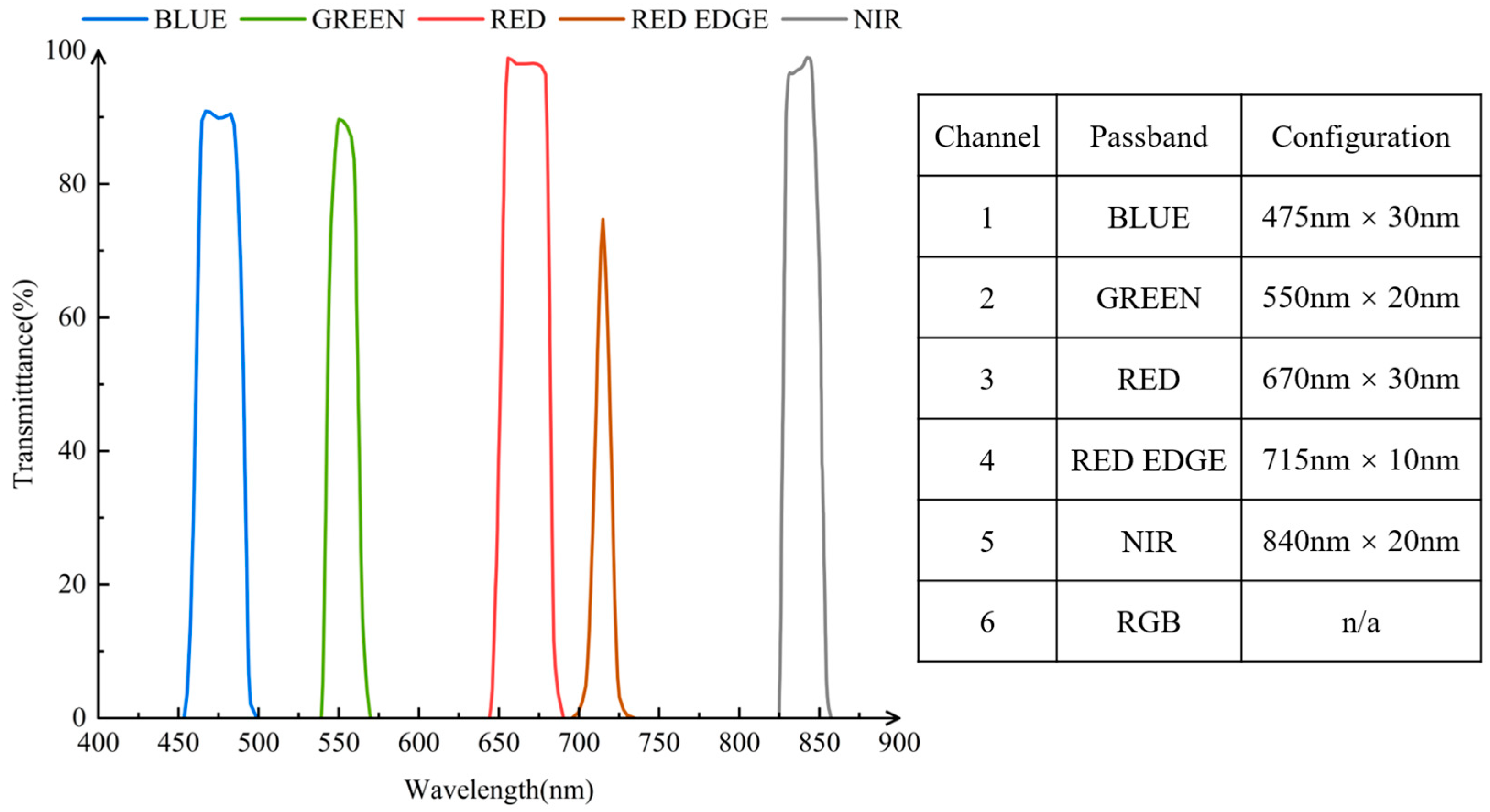
For validation analysis, high-precision drone data were collected using a 6X multispectral UAV, engineered in Minneapolis, MN, USA, 22 July 2021. The 6X multispectral UAV is equipped with six band channels: blue, green, red, red-edge, NIR, and RGB. These multispectral remote sensing images were acquired in July 2024 (Figure 2). Validation utilized UAV imagery classified via neural networks [16]. The measured areas were segmented to ensure uniform distribution of f_NPV measurements across low-to-high gradients (Figure 3).

The validation points from the UAV data were classified through the following procedure: the UAV imagery was segmented according to the target pixel resolution, and unidentifiable points, such as unavoidable clouds and shadows, were removed. Manual screening was then conducted using RGB composite previews of the UAV data to selectively identify points representing PV, NPV, BS, and distinct mixed vegetation–soil areas. The final selection was balanced to include nearly equal numbers of points from each of the four categories.

While UAV data provide valuable high-resolution validation, several limitations should be considered. The scale difference between UAV-derived pixels and satellite resolutions was mitigated by segmenting UAV imagery to match the satellite sensor’s resolution. Furthermore, although UAV coverage is spatially limited, flight campaigns were strategically designed to include representative landscapes such as oasis core areas, desert regions, and transition zones to enhance the ecological validity of the reference data.

2.1.3. Observed Field Data

The field-measured spectral data primarily consist of hyperspectral data for vegetation and soil, with reflectance as the measured index and a wavelength range of 350–2500 nm (

Table 1. Information on field measurement.

In Situ	Region	Description	Time	NPV/num	PV/num	BS/num
No.1	83°32′52″N, 44°1′43″E	Vegetation: Haloxylon, Nitraria, Calligonum; Soil: forest soil, cultivated soil, salinized soil.	20 July 2024	60	120	60
No.2	88°33′35″N, 44°48′43″E	Vegetation: Tamarix, Haloxylon ammodendro, Nitraria, Reaumuria soongorica; Soil: sandy soil, silty clay.	22 July 2024	45	90	15
No.3	101°18′5″N, 42°9′5″E	Vegetation: Tamarix, P. australis, Sophora alopecuroides; Soil: sandy soil.	31 July 2024	60	90	60
N0.4	100°53′42″N, 41°34′12″E	Vegetation: Populus euphratica, Tamarix, Alhagi, Sophora alopecuroide; Soil: sandy soil.	31 July 2024	100	90	60
N0.5	98°49′8″N, 39°57′43″E	Vegetation: Tamarix, Populus euphratica, Nitraria, Ephedra; Soil: gray-cinnamon soil, meadow soil.	9 August 2024	100	100	50
N0.6	99°40′12″N, 39°33′10″E	Vegetation: Tamarix, Sophora alopecuroides, Populus euphratica, Calligonum, Agriophyllum; Soil: gray-cinnamon soil, meadow soil.	9 August 2024	50	50	40
N0.7	102°54′46″N, 38°35′16″E	Vegetation: Nitraria, Calligonum, Haloxylon; Soil: sandy soil.	11 August 2024	90	100	60
N0.8	103°33′21″N, 39°1′33″E	Vegetation: Tamarix, P. australis, Chenopodium; Soil: moist soil, cinnamon soil.	11 August 2024	60	100	60
N0.9	81°19′33″N, 40°36′33″E	Vegetation: Populus euphratica, P. australis; Soil: aeolian sandy soil, meadow soil.	31 October 2024	30	50	30
N0.10	80°26′50″N, 41°25′52″E	Vegetation: Populus euphratica, Calligonum, Alhagi, Haloxylon; Soil: sandy soil, meadow soil.	31 October 2024	50	60	10
N0.11	86°17′12″N, 41°35′12″E	Vegetation: Populus euphratica, Calligonum, P. australis, Alhagi, Haloxylon; Soil: sandy soil, meadow soil.	2 November 2024	30	90	30
N0.12	92°23′4″N, 40°36′33″E	Vegetation: Populus euphratica, Calligonum, P. australis, Haloxylon; Soil: sandy soil, meadow soil.	4 November 2024	30	90	30

). The ASD spectrometer was used for this measurement, requiring dark current correction and optimization before measurement. In clear weather, a small whiteboard was used for reflectance calibration. An optical fiber was then used to align the feature for measurement [17]. The spectral measurement protocol was configured with 10 averaged scans per acquisition. For both target vegetation and soil measurements, five replicate scans were collected and averaged for each sample. Therefore, field spectral measurements were conducted primarily in arid zones with supplementary sampling in oasis areas, focusing on typical vegetation and soil targets.

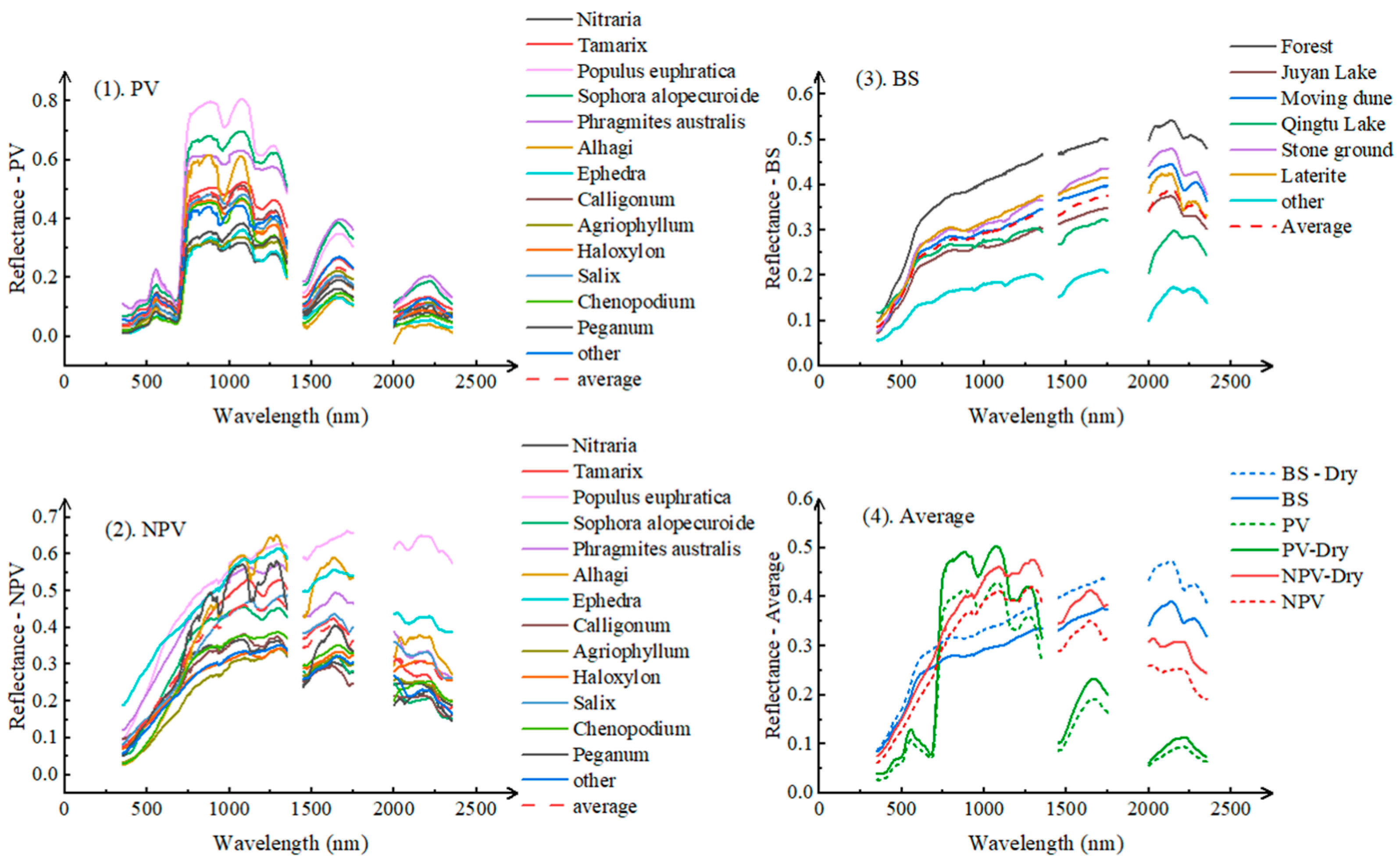
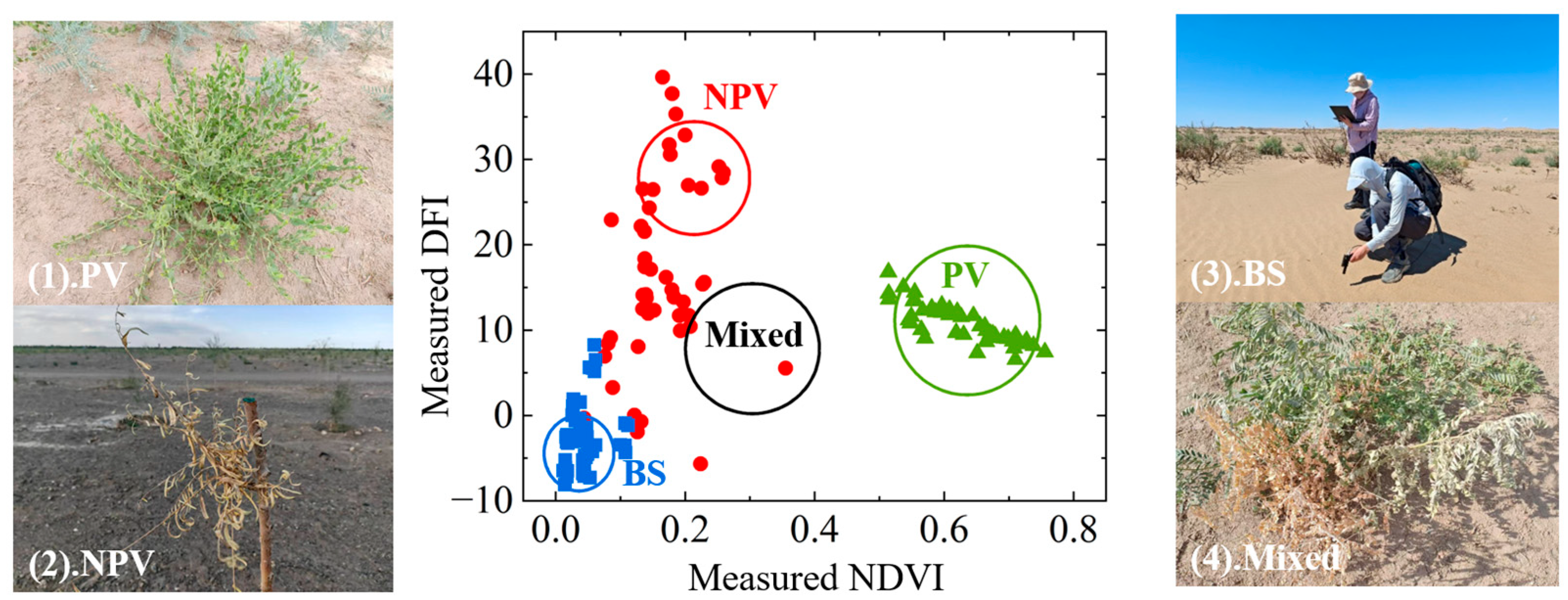
More than ten widely distributed dominant species were selected during fieldwork: Nitraria, Tamarix, Populus euphratica, Sophora alopecuroide, Phragmites australis, Alhagi, Ephedra, Calligonum, Agriophyllum, and Haloxylon, etc. In addition to the above vegetation spectrum information in arid areas, some vegetation in humid climate zones were also selected for research. Specific vegetation types and their spectral information are detailed in Figure 4. For spectral measurements, green leaves (PV) and yellowed leaves and large bare branches (NPV) were selected. Field spectral data were used to construct the feature space through commonly used spectral indices (Figure 5), specifically NDVI-DFI. In NDVI, PV > NPV > BS; In DFI, NPV > PV > BS; therefore, in the spectral index feature distribution of NDVI-DFI, the three components have obvious triangular spatial features, with PV in the lower right side of the triangle, NPV in the middle and upper end of the triangle, and BS in the lower left corner. Therefore, basic identification and classification can be achieved through the spectral characteristics of vegetation and soil under different vegetation indices. However, mixed pixel issues still exist for different land cover types (e.g., NPV and BS), requiring further selection and correction of vegetation indices.

2.2. Methods

2.2.1. Spectral Indexes

The preprocessing of spectra includes reading, checking, filtering, cropping, and resampling of hyperspectral data. Reflectance data were read, inspected, and averaged using the ViewSpecPro software. In the three wavelength ranges of 1350–1450 nm, 1750–2000 nm, and 2350–2500 nm, the water vapor is strongly absorbed, and three water vapor bands appear in these wavelength ranges, which need to be removed. Resampling refers to the convolution of the hyperspectral data [18]. To simulate the trend of spectral indexes in mixed scenarios, the selected spectral indices were divided into spectral indices of estimated PV and spectral indices of estimated NPV, and the specific formulas are shown in

Table 2. Spectral indices of simulated PV.

Index	Formula	References
NDVI	$(\mathit{NIR}-\mathit{RED})/(\mathit{NIR}+\mathit{RED})$	[21]
EVI	$2.5 \times ({\mathit{NIR}}_2-\mathit{RED})/({\mathit{NIR}}_2+6\times \mathit{RED}-7.5\times \mathit{BLUE}+1)$	[22]
MSAVI	$(2\times \mathit{NIR}+1)/2-\sqrt{{(2\times \mathit{NIR}+1)}^2-8\times (\mathit{NIR}-\mathit{RED})}$/2	[23]
LAIB	$-0.455+19.91\times (\mathit{SWIR}1-\mathit{SWIR}2)/(\mathit{SWIR}1+\mathit{SWIR}2)$	[13]
NDTI	$(\mathit{SWIR}1-\mathit{SWIR}2)/(\mathit{SWIR}1+\mathit{SWIR}2)$	[24]
STI	$\mathit{SWIR}1/\mathit{SWIR}2$	[25]

and

Table 3. Spectral indices of simulated NPV.

Index	Formula	References
DFI	$100\times (1-\mathit{SWIR}2/\mathit{SWIR}1)\times \mathit{RED}/\mathit{NIR}$	[26]
NSSI	$({\mathit{NIR}}_2-\mathit{REG})/({\mathit{NIR}}_2+\mathit{REG})$	[27]
NDSVI	$(\mathit{SWIR}1-\mathit{RED})/(\mathit{SWIR}1+\mathit{RED})$	[28]
SWIR32	$\mathit{SWIR}2/\mathit{SWIR}1$	[2]
NDI5	$(\mathit{NIR}-\mathit{SWIR}1)/(\mathit{NIR}+\mathit{SWIR}1)$	[24]
NDI7	$(\mathit{NIR}-\mathit{SWIR}2)/(\mathit{NIR}+\mathit{SWIR}2)$	[24]

. The selection of these spectral indices was informed by previous studies on vegetation and NPV spectral characteristics, particularly the work of Yuan, Luo et al. in the transition zone between the Minqin oasis and desert [19,20]. The indices were categorized into PV-oriented and NPV-oriented groups: NPV-oriented indices increase with higher non-photosynthetic vegetation cover, whereas PV-oriented indices increase with greater photosynthetic vegetation cover. To optimize the indices for NPV and PV estimation, field-measured spectra were convolved with sensor-specific spectral response functions to simulate coverage information representative of the study area. Each index was then evaluated through regression analysis against the simulated coverage data: NPV indices were tested against simulated NPV cover, while PV indices were assessed against simulated PV cover. This process ensured that the optimized indices exhibit strong, predictable responses to increasing fractional cover of their respective target components, thereby enhancing the separation between NPV and PV signals during spectral unmixing.

The performance of the model was evaluated by the coefficient of determination (R²) and the root mean square error (RMSE) as shown in Equations (2) and (3) below.

$$R^2={\left({\sum }_{i=1}^n\left(X_i-\overline{X}\right)\left(Y_i-\overline{Y}\right)\right)}^2/{\sum }_{i=1}^n{\left(X_i-\overline{X}\right)}^2{\sum }_{i=1}^n{\left(Y_i-\overline{Y}\right)}^2$$

(1)

$$\mathit{RMSE}=\sqrt{{\sum }_{i=1}^n{(X_i-Y_i)}^2/n}$$

(2)

where Xi and Yi are the simulated and measured values, $\overline{X}$ and $\overline{Y}$ are the means of the simulated and measured values, respectively, and n is the sample number.

The choice of R² and RMSE as the core validation metrics was based on the characteristics of the UAV-derived validation data and the specific requirements of model evaluation. R² measures the consistency between model predictions and UAV observations, reflecting how well the spectral mixture analysis model reproduces the spatial distribution patterns of PV and NPV cover. This is ecologically significant, as the spatial arrangement of vegetation directly influences ecosystem functioning. RMSE quantifies the absolute error in coverage estimation at the pixel level, which is essential for assessing the practical utility of the inversion results.

2.2.2. Optimized Spectral Mixture Analysis Model

The data framework for arid-zone field collections appears in Figure 1. Model derivation workflows proceed through these stages: (1) The processed spectra data. To develop the model and evaluate model parameters, spectral data require preprocessing to construct spectral datasets. Dual datasets were established: one modeling mixed-endmember scenarios across fractional gradients, another adopting administrative partitioning with regional spectral libraries. The preprocess employed response function convolution (Equation (3)) for sensor-specific calibration:

$$\overline{\rho }={\int }_{{\lambda }_1}^{{\lambda }_2}\rho \left(\lambda \right)·s\left(\lambda \right)d\lambda /{\int }_{{\lambda }_1}^{{\lambda }_2}s\left(\lambda \right)d\lambda$$

(3)

where $\overline{\rho }$ is the simulated satellite band reflectivity, $s\left(\lambda \right)$ is the spectral response function of different remote sensing sensors, ${\lambda }_1$ and ${\lambda }_2$ are the lower and upper limits of the corresponding bands, and $\rho \left(\lambda \right)$ is the collected hyperspectral data (Figure 6).

For the spectral dataset, the vegetation spectral information was derived from the average spectra of field dominant species, while the BS spectral information was selected from the average field soil spectra across multiple sites. The fractions of PV (f_PV), NPV (f_NPV), and BS (f_BS) were varied within the range of 0 to 1, with a step size of 0.1. Consequently, the variation in (f_PV, f_NPV, f_BS) spanned from (0.0, 0.0, 1.0) to (1.0, 0.0, 0.0), yielding a total of 66 simulated spectra with distinct coverages.

(2) The model development. Traditional spectral mixture analysis, a commonly used method for mixed image element decomposition, has been extensively applied in the estimation of NPV and PV fractional cover in arid and semi-arid regions globally [29]. Spectral mixture analysis assumes that the mixed image is a linear combination of the information from PV, NPV, and BS within the image, with the proportions of the image area they occupy serving as weighting coefficients [30]:

$$R\left(\lambda \right)=(f_{\mathit{PV}}{R\left(\lambda \right)}_{\mathit{PV}}+f_{\mathit{NPV}}{R\left(\lambda \right)}_{\mathit{NPV}}+f_{\mathit{BS}}{R\left(\lambda \right)}_{\mathit{BS}})$$

(4)

$$\sum f=f_{\mathit{PV}}+f_{\mathit{NPV}}+f_{\mathit{BS}}=1$$

(5)

where R(λ) is the spectral index of a pixel in the remote sensing image, f_PV, f_NPV, f_BS are the pixel distribution percentages of PV, NPV, and BS within the corresponding pixel, and R(λ)PV, R(λ)NPV, and R(λ)BS are the spectral index values of the three types of pure endmembers within the corresponding pixel, respectively. Equations (4) and (5) show the processing of the pixel values within the feature space, and the anomalous pixel values need to be processed with the following formulas:

$$C_x=\left\{\begin{array}{c}0,(-0.2<C_x<0)\\ 1,(1<C_x<1.2)\end{array}\right.$$

(6)

$$C_y=C_y/(C_y+C_z)$$

(7)

$$C_z=C_z/(C_z+C_y)$$

(8)

$$C_x=C_y=C_z=0,(C_x<-0.2\mathit{or}{C}_x>1.2)$$

(9)

Traditional models utilize globally uniform spectra across all regions. To overcome this limitation, globally invariant spectra are replaced by spectrally diverse datasets incorporating spatial constraints. The study area is partitioned into K administrative subregions, each allocated a dedicated spectral dataset. Within each subregion, regional instances of the primary spectral dataset are constructed. Subsequently, all regional spectra undergo standardization according to Equation (10), normalized to a mean of $r_i\left(\lambda \right)$ and standard deviation of ${\sigma }_i\left(\lambda \right)$. The parameter information of the model is provided in

Table 4. Definitions and significance of variables for the spectral mixture analysis model.

Variables	Definitions	Significance
R(λ)	The spectral index of a pixel	Used for spectral unmixing, with values varying across different regions.
Cx, Cy, Cz	Anomalous pixel values of different land covers	Reduces the impact of anomalous pixels.
$r_i\left(\lambda \right)$	Spectral mean of the sub-region	Unifies the spectral characteristics within sub-regions.
$e_i^K\left(\lambda \right)$	Endmember	Serves as a critical variable in pixel decomposition, representing the distinctive spectral values of different land cover types.
${\delta }_i\left(x,y\right)$	The fluctuation term of the i-th endmember	Represents spatial heterogeneity.

.

$$R_i^K\left(\lambda \right)=(e_i^K\left(\lambda \right)-r_i\left(\lambda \right))/{\sigma }_i\left(\lambda \right)$$

(10)

Using NPV as an example, spatial covariance matrices were developed to generate controlled spectral variations among administrative subregions:

$${\sum }_S^{\mathit{NPV}}={\displaystyle \frac{1}{K}}{\sum }_{K=1}^K(R_i^{\mathit{NPV}}\left(\lambda \right)-r_{\mathit{NPV}}){(R_i^{\mathit{NPV}}\left(\lambda \right)-r_{\mathit{NPV}})}^T$$

(11)

The optimized model incorporating spatial constraints is expressed as:

$$R(x,y)={\sum }_{i=1}^3{f}_i\left(x,y\right)\left(e_i^0+{\delta }_i\left(x,y\right)\right)+\epsilon (x,y)$$

(12)

where $e_i^0$ denotes the baseline endmember, and ${\delta }_i\left(x,y\right)$ represents the fluctuation term of the i-th endmember at location $\left(x,y\right)$, subject to spatial covariance constraints.

3. Results

3.1. Optimization of Vegetation Index

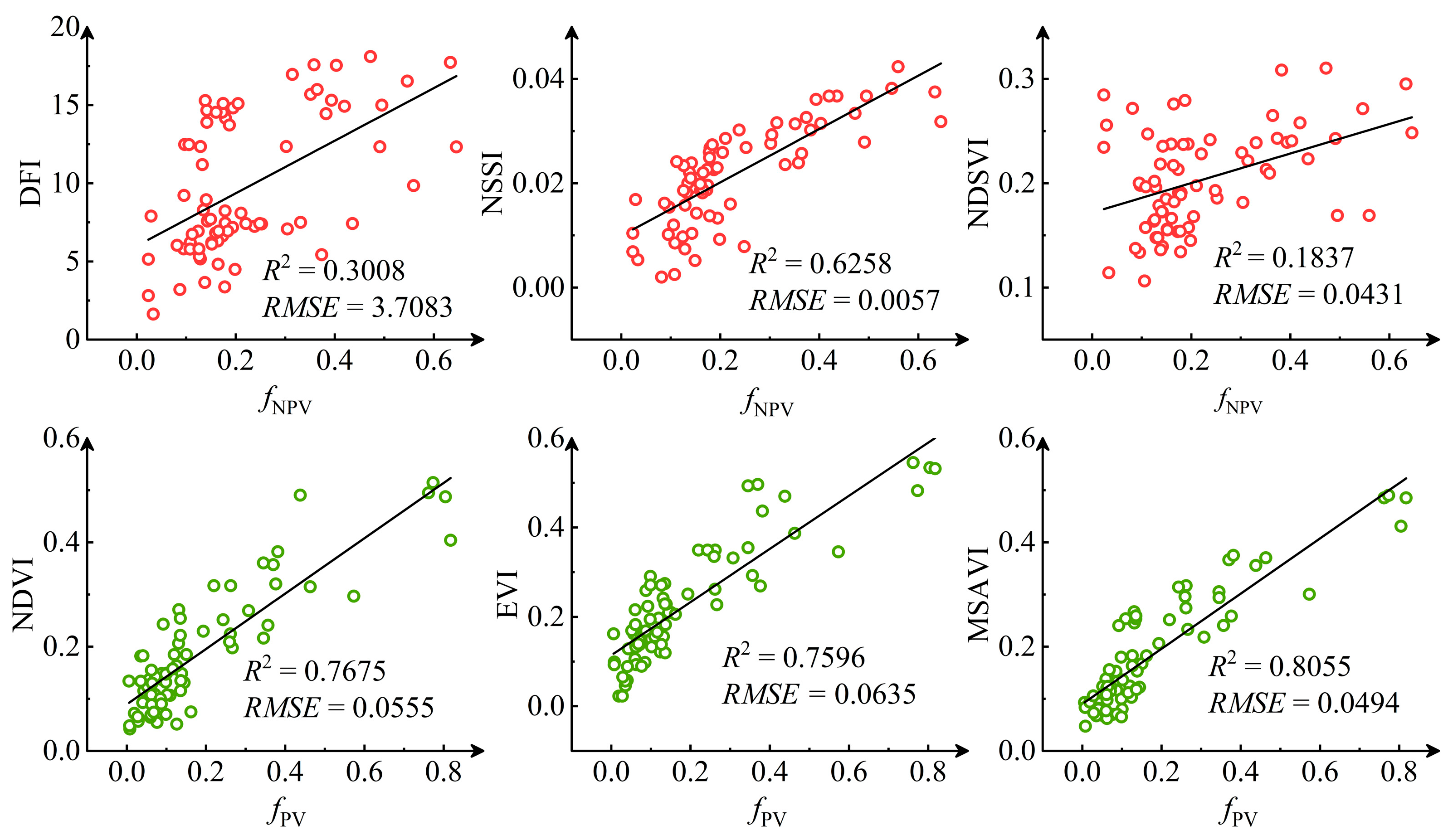
Vegetation index selection requires systematic optimization. Correlation analysis was performed between spectral indices of PV/NPV and their simulated coverage fractions using baseline endmember $e_i^0$. Underperforming indices were subsequently optimized and validated based on analytical outcomes.

Table 5. The simulated results of the index with f_NPV and f_PV in Sentinel-2.

NPV	Regression Formula	R2	RMSE	PV	Regression Formula	R2	RMSE
DFI	y = 0.1160fNPV + 0.0568	0.5443 *	0.0285	NDVI	y = 0.5775fPV + 0.1111	0.9667 *	0.0253
SWIR32	y = 0.0347fNPV + 0.0876	0.0098	0.0936	EVI	y = 0.6036fPV + 0.0965	0.9638 *	0.0314
NDSVI	y = 0.0653fNPV + 0.2707	0.1092 *	0.0501	MSAVI	y = 0.4421fPV + 0.1214	0.9739 *	0.0236
NSSI	y = 0.0398fNPV + 0.0111	0.9071 *	0.0034	LAIB	y = 0.4582fPV + 0.0451	0.6465 *	0.0911
NDI5	y = −0.1781fNPV + 0.1273	0.1450 *	0.1162	NDTI	y = 0.0233fPV + 0.1145	0.0066	0.0766
NDI7	y = −0.1349fNPV + 0.2276	0.0389	0.1802	STI	y = 0.0145fPV + 1.2924	0.0003	0.2153

Regression analysis, * p < 0.01.

lists the simulations of various commonly used indices of Sentinel-2 to the coverage when in the mixed NPV-PV-BS scenario, which exhibit distinct spectral features when encountering NPV. Table 4 shows that DFI, NDSVI, and NSSI increase with the increase of f_NPV, while SWIR32, NDI5, and NDI7 decrease with the increase of f_NPV, and these four indices are feasible to estimate f_NPV. Meanwhile, the two spectral indices, DFI and NSSI, had an R² of greater than 0.5 and an R² of determination of NSSI higher than 0.9 with the smallest fitting error. The coefficients of determination of NDI5 and NDSVI were less than 0.2.

Among the indices being fitted to f_PV, all four indices had linear relation to the f_PV with an R² of over 0.6 and all increased with f_PV, proving the feasibility of the four indices to estimate f_PV. However, the simulated LAIB results were relatively poor, and the errors were relatively the highest. The R² values of EVI, MSAVI, and NDVI were all greater than 0.9, among which the MSAVI had the highest R² and the lowest error since it was less affected by the NPV and BS. The remaining two metrics, NDTI and STI, did not pass the significance test and are not applicable to the estimation of f_PV. Using the same analytical method, the indices of MODIS and Landsat data were analyzed; the simulated results for MODIS are shown in

Table 6. The simulated results of the index with f_NPV and f_PV in Landsat8.

NPV	Regression Formula	R2	RMSE	PV	Regression Formula	R2	RMSE
DFI	y = 0.1132fNPV + 0.0568	0.5129 *	0.0296	NDVI	y = 0.5629fNPV + 0.1038	0.9562 *	0.0324
SWIR32	y = −0.0608fNPV + 0.8117	0.0183	0.1198	EVI	y = 0.4595fNPV + 0.0972	0.9472 *	0.0292
NDI5	y = 0.1634fNPV − 0.1341	0.1206 *	0.1186	MSAVI	y = 0.5530fNPV + 0.1294	0.9571 *	0.0315
NDSVI	y = 0.1174fNPV − 0.2321	0.0291	0.1822	LAIB	y = 0.4575fNPV + 0.0441	0.6385 *	0.0925

Regression analysis, * p < 0.01.

, and those for Landsat-8 are shown in

Table 7. The simulated results of the index with f_NPV and f_PV in MODIS.

NPV	Regression Formula	R2	RMSE	PV	Regression Formula	R2	RMSE
DFI	y = 0.1132fNPV + 0.0518	0.3398 *	0.0424	NDVI	y = 0.4484fPV + 0.1001	0.9444 *	0.0292
SWIR32	y = −0.0526fNPV + 0.8119	0.0099	0.1417	EVI	y = 0.5346fPV + 0.1039	0.9532 *	0.0318
NDI5	y = 0.1625fNPV − 0.1211	0.1284 *	0.1138	MSAVI	y = 0.5392fPV + 0.1336	0.9535 *	0.0220
NDSVI	y = 0.1253fNPV − 0.2222	0.0301	0.0301	LAIB	y = 0.5597fPV + 0.0105	0.6772 *	0.1038

Regression analysis, * p < 0.01.

.

Simulated results indicate that R² for f_NPV was relatively low under theoretical simulation, with DFI, NDSVI, and NDI5 exhibiting a positive correlation with f_NPV. In Sentinel data fitting validation, the R² of NSSI reached 0.9071; however, the high-precision Sentinel data’s cloud cover and update frequency were insufficient to meet large-scale inversion calculations during the vegetation growing season. Therefore, simulated correction and reconstruction of drought indices from medium-resolution sensors are required to enhance the applicability of parameters across diverse climatic regimes.

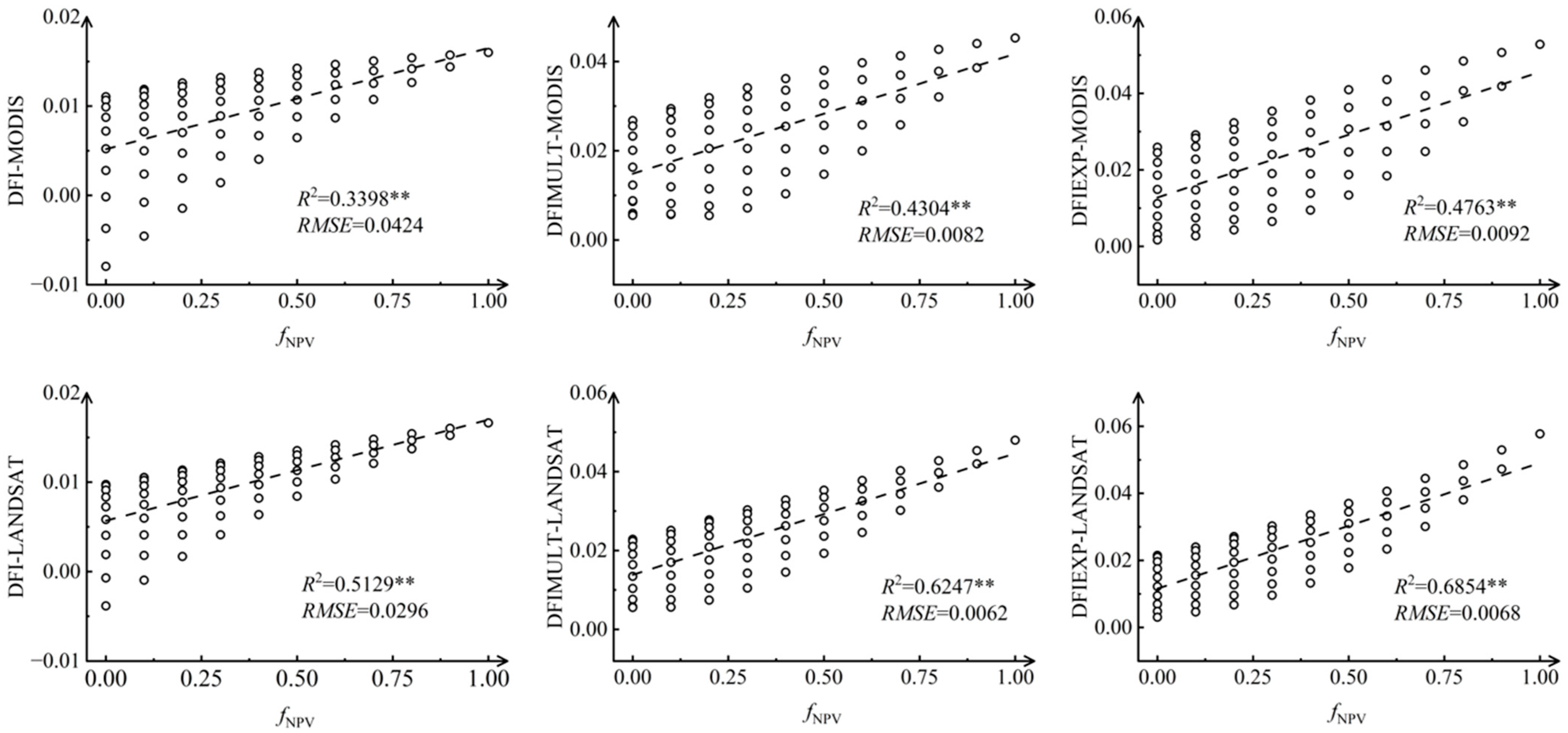
Using the positive correlation trend between DFI and both NSSI and f_NPV in Sentinel data, simulated correction was performed. After normalization, polynomial and exponential fitting were conducted, and the simulated indices were designated as DFIMULT and DFIEXP, with the formulas as follows:

$${DFI}_{MULT}=116.25\times {DFI}^2+0.5849\times DFI+0.0061$$

(13)

$${DFI}_{EYP}=0.0053\times e^{143.61\times DFI}$$

(14)

Based on the comparative results of optimized fitting validation, see Figure 7.

To validate the corrected indices, MODIS and Landsat8 data were selected for validation. The f_NPV distribution at 10 m spatial resolution was calculated using Sentinel-2A image data, followed by upscaling to 30 m and 500 m resolutions to match the pixel sizes of Landsat 8 and MODIS images. To upscale remote sensing data from finer to coarser spatial resolution, the 10 m resolution Sentinel-2 raster data were resampled to 30 m and 500 m resolutions, respectively, to ensure spatial consistency, and then cross-validated with Landsat and MODIS data accordingly [31].

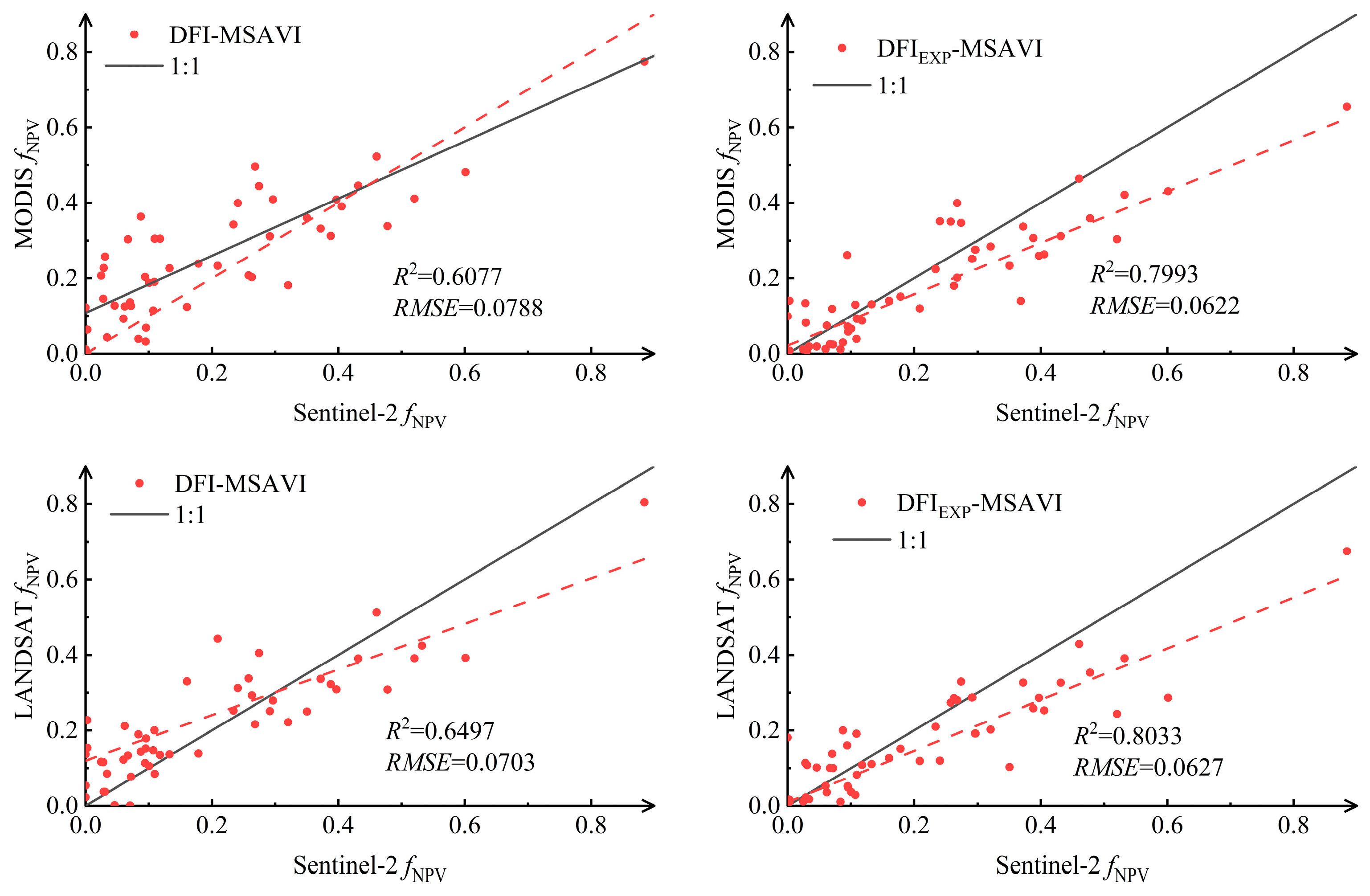
Then, 50 validation points were randomly distributed. Under theoretical conditions, the DFIEXP index demonstrated optimal fitting performance. Consequently, the estimation results of the f_NPV remote sensing models based on both DFI and DFIEXP indices were comparatively analyzed with scale-consistent MODIS-FNPV and Landsat-FNPV products, respectively. The validation results are presented in Figure 8, while comparative raster maps of inversion results for selected regions are shown in Figure 9.

The validation scatter plots clearly demonstrate that significant overestimation of vegetation coverage occurs when employing the uncorrected DFI index for inversion of low f_NPV values. Landsat 8 achieved a determination coefficient of 0.6077 while MODIS reached 0.6497, with data points scattered unevenly around the 1:1 reference line, indicating substantial deviations from Sentinel values (Figure 8). After the index correction, the model performance improved markedly, with the corrected DFI index yielding significantly higher determination coefficients of 0.7993 for Landsat 8 and 0.8033 for MODIS data, thereby confirming the effectiveness of the correction approach. These quantitative improvements align perfectly with the spatial patterns observed in the remote sensing imagery presented in Figure 9.

3.2. Calibration and Verification

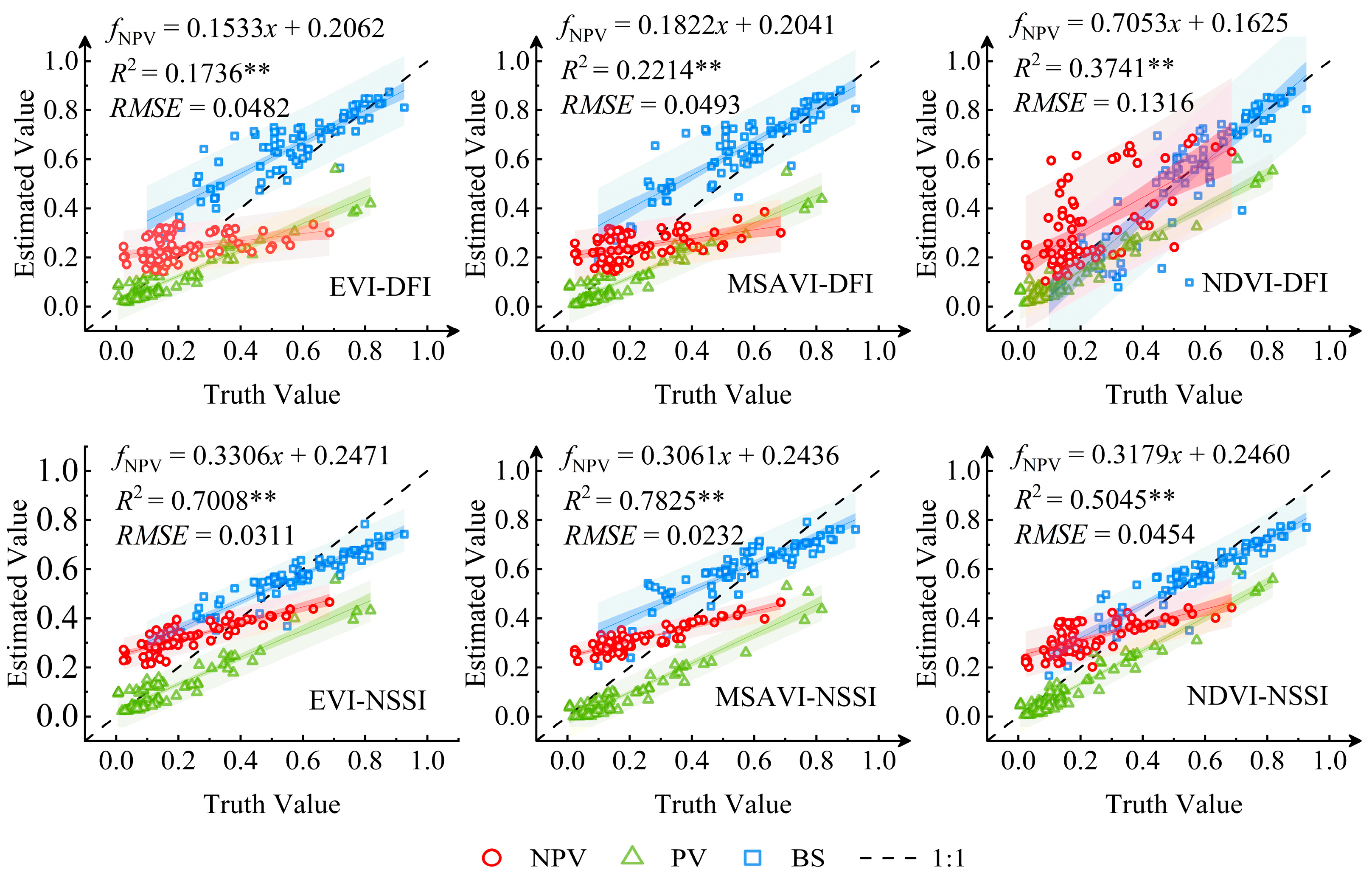
Leveraging optimized model parameters and sensor configurations, spectral indices demonstrating superior fitting performance (EVI-DFI, EVI-NSSI, MSAVI-DFI, MSAVI-NSSI, NDVI-DFI, NDVI-NSSI) were selected for fractional cover inversion, with validation conducted using UAV imagery. Across three study areas, a total of 75 sampling points were collected for validation and evaluation, covering regions with high, medium, and low vegetation coverage to mitigate overfitting. The UAV validation results are presented in Figure 10.

Among them, MSAVI-NSSI had the highest R² of 0.7825, which was also higher than that of the linear regression model established by using only the DFI index, and the RMSE was the lowest at 0.0232. Therefore, MSAVI-NSSI could be selected as the parameter and the ternary linear mixed model could be used to conduct the inversion and estimation. Among them, the R² of f_PV reached 0.8725, and the RMSE was 0.0063. Using the average of all endmember values as the model’s baseline endmember values, the endmember values of different sensors are shown in

Table 8. Corrected baseline endmember values.

Sensor	Sentinel-2A		Landsat8 OIL		MODIS
Index	MSAVI	NSSI	MSAVI	DFIEXP	MSAVI	DFIEXP
PV	0.6183	0.0188	0.5731	0.0209	0.5629	0.0258
NPV	0.1836	0.0687	0.1638	0.0717	0.1664	0.0728
BS	0.0461	−0.0024	0.0369	0.0031	0.0821	0.0017

The endmember values in the table serve as the baseline endmember values for field-observed spectral data, representing the spectral characteristic information employed in conventional spectral mixture analysis algorithms.

.

Then, an empirical vegetation index model was established based on the UAV-measured f_NPV and the spectral index under the Sentinel-2 remote sensing image in the same period, and in order to avoid the phenomenon of overfitting, the selected sample of measured points contained high-coverage and low-coverage areas and oasis and desert areas—the results are shown in Figure 11. The R² value of the obtained results was slightly lower than that of the simulated data, which was mainly affected by a variety of complex environmental factors such as rivers, biological activities, and human activities. These results indicate that the empirical vegetation index models are less applicable to large-scale regions compared to the spectral mixture analysis model.

A comparison of the two inversion methods shows that the optimized spectral mixture analysis model yields better validation results than the empirical vegetation index-based model, and outperforms single-index calculations in estimating both NPV and PV coverage. Here, PV can serve as an indicator of vegetation greenness, and the higher R² value compared to that achieved using direct vegetation indices such as NDVI suggests that the method also offers an improved approach to retrieving vegetation greenness. Moreover, the effective separation of senescent vegetation from healthy green vegetation allows for future application of change detection methods to independently monitor changes in PV and NPV coverage. This capability can provide a better foundation for assessing vegetation health in arid regions.

3.3. Inversion Results

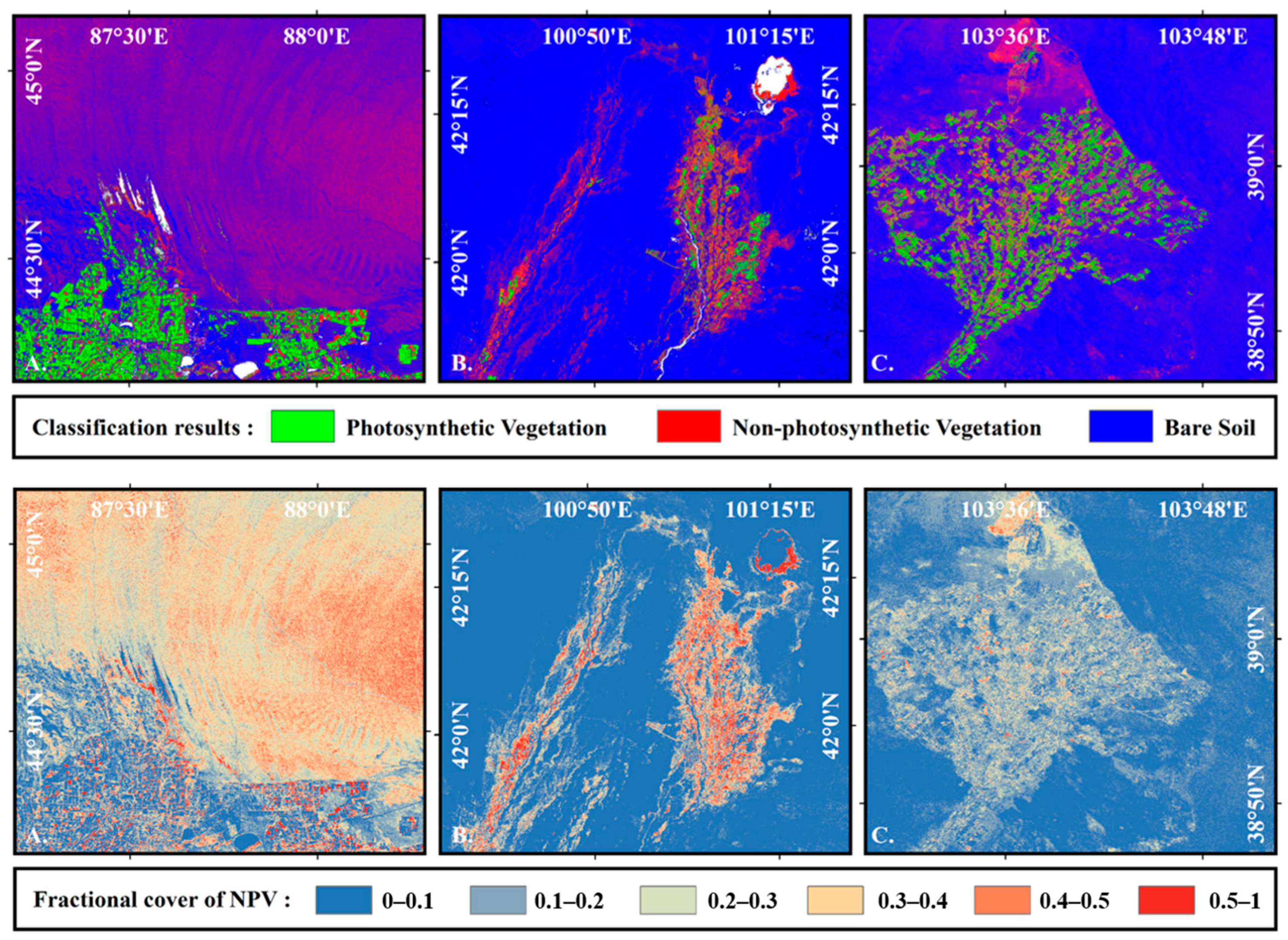
The optimized linear mixing model using MSAVI-NSSI parameters demonstrates effective performance in high spatial resolution small-area inversion, as shown in Figure 12. In the Sentinel-2A inversion results, blank or missing values mainly correspond to water bodies such as lakes and land cover types outside the triplet components. For example, the Heihe River, after water diversion, flows through the Ejina Banner in Inner Mongolia and crosses the oasis region along the southern margin of the Junggar Basin, including reservoirs and terminal lakes. The East Juyanhai lake area in northern Ejina Banner also exhibits these blank values. In contrast, the Qingtu lake region contains small, reed-covered water surfaces, which do not produce significant blank pixels in the inversion results.

In the Junggar Basin, most of the oasis farmland is characterized by PV, and most of the desert area is characterized by NPV and BS. Among them, the senescent mature wheat and maize post-harvest stumps and fallow land in the oasis area produce the characteristics of NPV, thus leading to the distribution of NPV in the farmland area in the form of block-area type. The Ejinagi Banner region in Inner Mongolia belongs to the lower reaches of the Heihe River and the vegetation growth and health condition are lacking, and the NPV accounts for a high percentage, with a large number of artificially constructed poplar forests and manmade forests around Ejinagi Banner, so the inversion results show photosynthesizing vegetation. The Qingtu lake region located at the lower reaches of the Shiyang River has been called to make efforts in the control of sand and afforestation in recent years, and the proportion of PV in this area is therefore high.

The three selected regions span from arid to semi-arid zones, covering different degrees of aridity from the deserts of Xinjiang to the lower and upper reaches of the Heihe River. The inversion results from the optimized spectral mixture analysis model show a gradually decreasing proportion of NPV pixels across these regions, which aligns with the actual conditions of different arid areas. This spatial pattern reflects the health status of vegetation growth across various arid zones and indirectly indicates regional aridity levels. Additionally, the model effectively separates water body information.

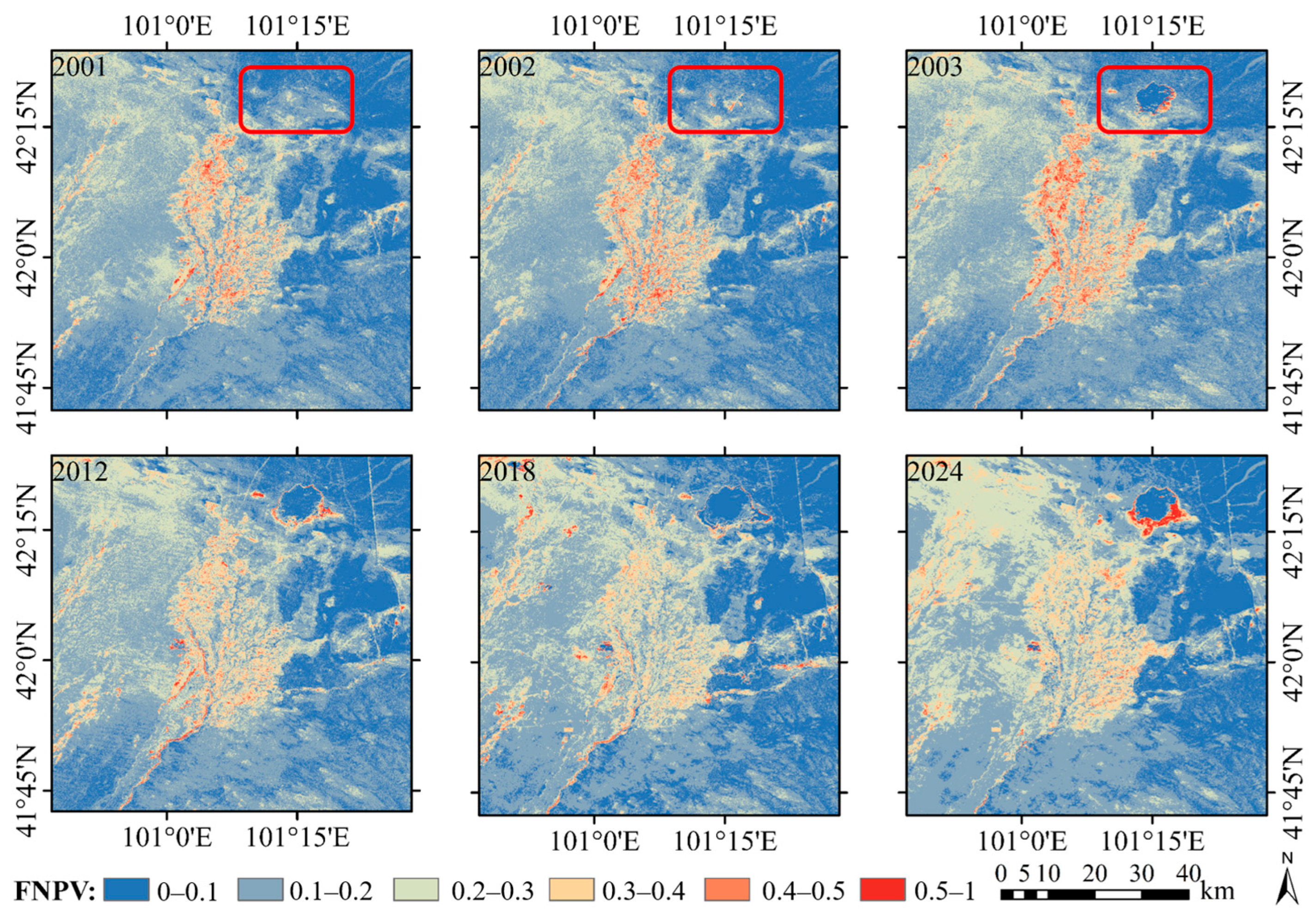
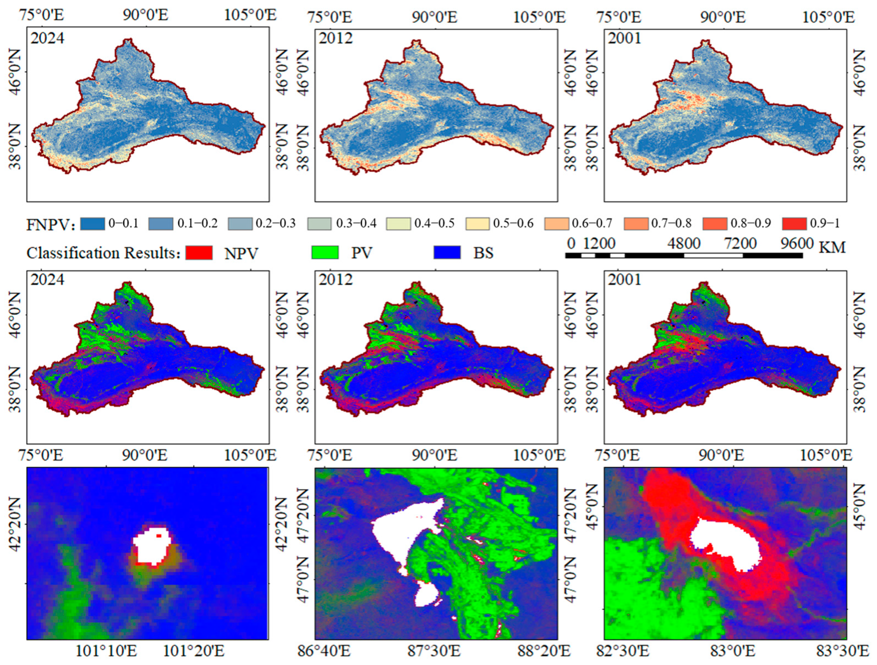
The inversion results derived from Landsat 8 data for selected regions are presented in Figure 13, while Figure 14 displays the corresponding results obtained from MOD09GA data across the entire inland river basins of China. Among these, according to the inversion data from Landsat8, Juyan Lake was in a dry state in 2001 and 2002, but regained vitality in 2003, which aligns with the actual evolutionary history of Juyan Lake. The model demonstrates effective capability in identifying regional land cover changes, making it suitable for long-term monitoring of the NPV dynamics and ecological health assessment. The model demonstrates effective capability in identifying regional land cover changes. It successfully discriminates between various vegetation and soil types while also effectively separating water bodies. This makes it suitable for long-term monitoring of dynamic changes in Juyan Lake and for assessing the ecological health of surrounding vegetation.

The identification results from MODIS data demonstrate that in 2024, both the Taklimakan Desert in southern Xinjiang and parts of northern Xinjiang exhibited a significant decrease in bare soil and NPV coverage compared to 2012 and 2001, while showing a notable increase in photosynthetic vegetation. Major terminal lakes including Juyan lake, Ulungur lake, and Ebinur lake were accurately identified, demonstrating the model’s capability in water body detection across arid areas. This indicates an improvement in local vegetation ecological health, where photosynthetically active green vegetation is progressively replacing non-photosynthetic withered vegetation and bare soil. Consequently, these parameters can serve as crucial indicators for monitoring vegetation ecological health in arid areas. Although the spatial resolution of the MODIS remote sensing sensor is coarser than that of Landsat and Sentinel-2 sensors, its 8-day revisit imagery still enables the identification of NPV and the effective separation of water bodies. Therefore, MODIS can serve as a primary sensor for large-scale monitoring of vegetation ecological health.

3.4. Optimization of Spectral Constraint Weights for Key Phenological Stages

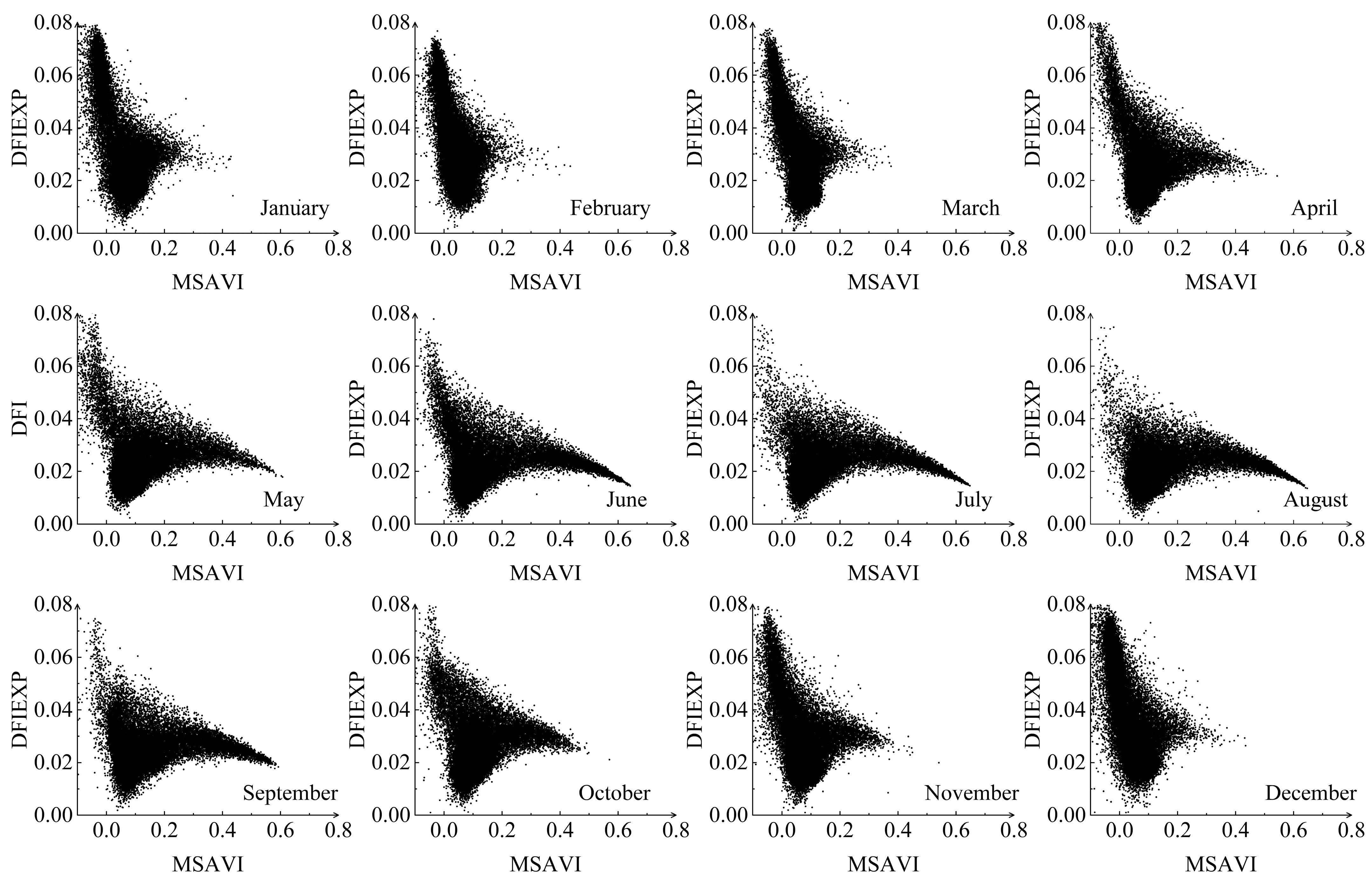
Under the optimization of spectral libraries, NPV during the growing season can be more effectively identified. However, addressing the requirements of long-term time series data involves challenges due to varying spectral characteristics under different phenological conditions. Collecting spectral information across all phenological stages entails substantial effort. Therefore, it is feasible to correct endmember values for various phenological stages in remote sensing by referencing endmember values from spectral libraries, incorporating spectral constraint weights. Accordingly, for arid regions in China, MODIS data were selected to statistically analyze endmember values across phenological stages. Endmember values from the same calendar date each month between 2020 and 2024 were averaged, and weights were ultimately calculated based on reference endmember values from spectral libraries. The spectral endmember values for different months are illustrated in Figure 15.

As observed from the spectral scatter distribution, vegetation enters a dormant period from December to February, characterized by sparse pixel distribution in the PV region and a dominant proportion of NPV. From March to April, vegetation enters the initial growth stage, showing signs of greening and an increase in PV pixels. Rapid growth begins in May and remains stable until August, representing the steady growth phase. From September to October, vegetation transitions into senescence, with aging plants leading to a noticeable rise in NPV pixels. From November to December, vegetation progresses into a completely withered state. Phenological changes are closely associated with air temperature, precipitation, and soil moisture, consequently leading to variations in the coverage of both PV and NPV. Accordingly, weighting calculations based on reference spectra from the growing season were performed, and the results are presented in

Table 9. Spectral constraint weights.

	Feature Type	Month
		1	2	3	4	5	6	7	8	9	10	11	12
PVI	PV	1.9036	3.0946	2.1194	1.2964	0.9872	0.8782	0.8687	0.8849	0.9634	1.1621	1.5140	1.7791
	NPV	−1.2597	−1.2635	−1.1358	−1.3248	1.4910	1.1954	1.2830	1.0472	1.5923	−1.4259	−1.3238	−1.2208
	BS	1.4204	1.4253	1.9138	1.6824	1.7176	1.4058	1.8830	1.6755	1.4034	1.4609	1.9501	2.1105
	PV	0.8805	0.8088	0.8459	1.0574	1.2709	1.6863	1.7793	1.7917	1.3368	0.9961	0.8990	0.8012
NPVI	NPV	0.9345	0.9746	0.9455	0.9825	1.1115	1.1357	1.1974	0.1056	1.0882	1.0643	0.9973	0.9467
	BS	0.2982	0.3036	0.3778	0.2742	0.3148	0.5862	0.3542	0.5313	0.3333	0.4146	0.3617	0.2073

PVI refers to the PV Index, while NPVI refers to the NPV Index.

.

4. Discussion

4.1. Development of a Spectral Angle Mapper (SAM) Model Based on Multiple Ecoregions

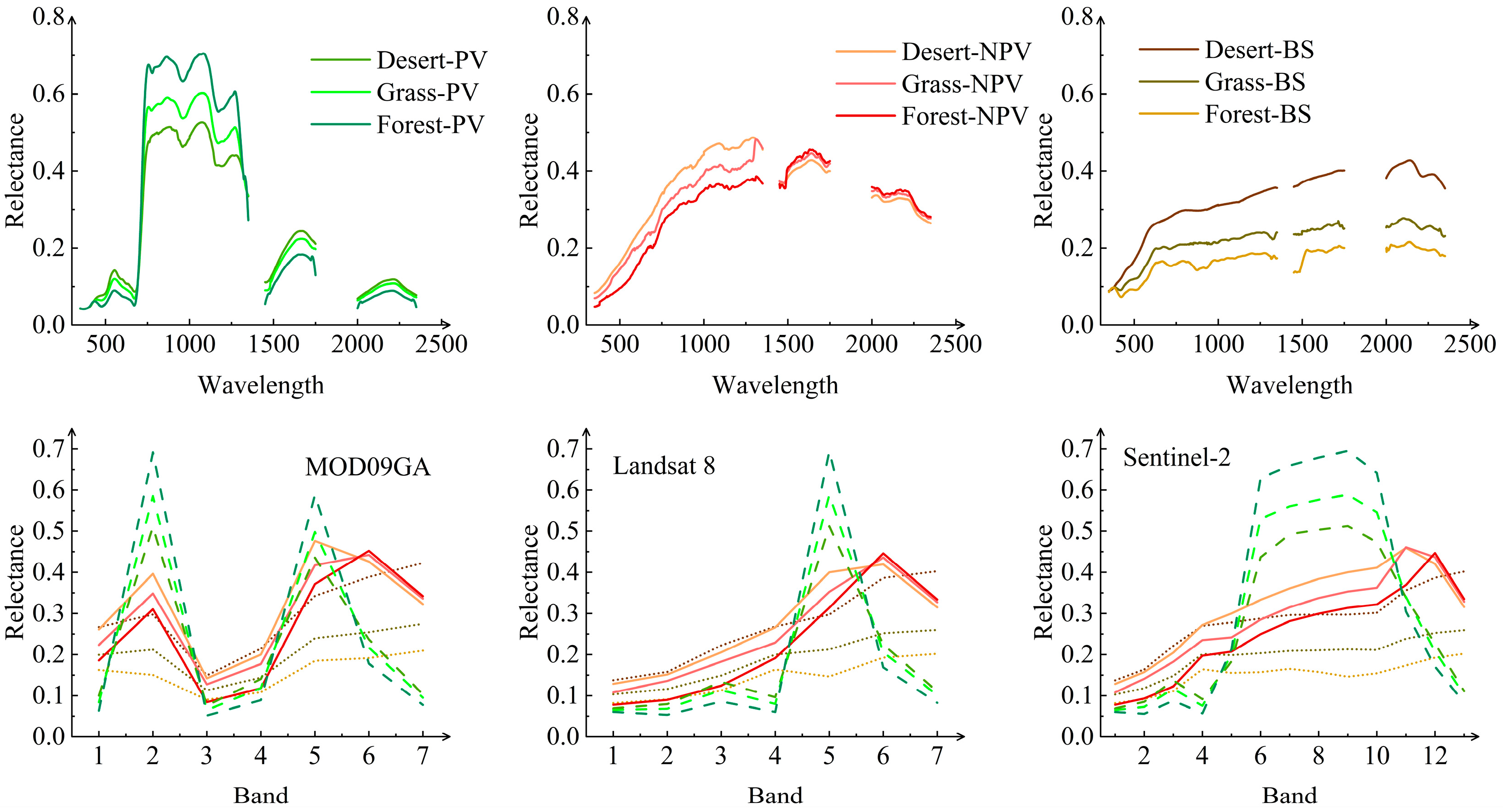
The primary ecoregion of focus in this study is the arid zone. Therefore, all spectral data were collected from arid regions, and only spectral datasets and spectral matrices specific to arid zones were constructed, ensuring the model is fully applicable to such environments. However, other ecological environments on Earth, such as temperate grasslands and forest ecoregions, also feature withered meadows, dry branches, and fallen leaves. To account for this, spectral data from Wang and Zhu’s research on grasslands in Inner Mongolia and forests in Chuzhou [3,20], as well as data from the USGS Spectral Library Version 7 [32], were referenced. Additional spectral data were incorporated for grassland species including Stipa capillata, Achnatherum splendens, Artemisia spp., Cleistogenes squarrosa, Bromus inermis, Nassella tenuissima, and for forest species such as Populus spp., Populus euphratica, Picea engelmannii, Pinus banksiana, Acer spp., and Quercus robur. The ecoregions were broadly categorized into arid zones, temperate semi-arid grasslands, and subtropical forests. The average spectral values were used as baseline reference spectra and convolved into the Sentinel-2, Landsat 8, and MODIS sensors according to Equation (3), as illustrated in Figure 16.

As observed from the spectral curve comparison, for the PV spectral curves, the forest exhibits the lowest reflectance in the visible region, followed by grassland, and the arid zone has the highest. This pattern is attributed to the dense forest canopy absorbing more photosynthetically active radiation, while vegetation is sparse in arid regions. In the near-infrared region, the forest shows the highest reflectance, followed by grassland, with the arid zone having the lowest. This is likely due to the lush foliage in forests causing multiple scattering. In the shortwave infrared region, the forest has the lowest reflectance, followed by grassland, and the arid zone has the highest. This is analyzed to result from the high water content in forests leading to lower reflectance, whereas vegetation in arid regions, under persistent water stress with low water content, exhibits the highest reflectance. For the NPV curves, in the near-infrared and shortwave infrared regions, the arid zone has the lowest reflectance, while forests have the highest. This is analyzed to be because arid regions are more susceptible to influences from the ground surface. For the BS curves, the arid zone overall shows the highest reflectance, and forests the lowest, which is primarily due to the effect of moisture.

Therefore, building upon the establishment of spectral databases and matrices for individual ecoregions, the framework has been expanded to incorporate multiple ecoregions. By integrating benchmark reference spectra from different ecological zones along with an indicator for evaluating spectral similarity, optimal endmembers can be selected across various regions, thereby enhancing the generalizability of the algorithm. Based on the reference spectra, the Spectral Angle Mapper (SAM) is constructed, Equation (15), which calculates the inverse cosine of the cosine value between two spectral vectors [33]:

$$\theta ={\cos }^{-1}\left(\frac{{\displaystyle {\sum }_{i=1}^n(T_i·R_i)}}{{\displaystyle \sqrt{{\sum }_{i=1}^n·T_i^2}·\sqrt{{\sum }_{i=1}^n·R_i^2}}}\right)$$

(15)

where θ represents the spectral angle to be determined, measured in degrees, and n denotes the number of bands. T_i is the reflectance value of the first spectral curve at the i-th band, while R_i is the reflectance value of the second spectral curve at the i-th band. A smaller θ value indicates that the two spectral curves have more similar shapes and are more likely to correspond to the same type of surface feature. Conversely, a larger θ value suggests greater dissimilarity in the shapes of the two curves, indicating a higher likelihood that they represent different surface features.

Three sites were selected for validation: a desert site in the Junggar Basin for Sentinel-2, a senescent grassland area in Inner Mongolia for Landsat 8, and a forest region in Anhui for MODIS. The specific geographic coordinates and corresponding validation results are presented in

Table 10. SAM validation results.

Site	Sensors	Region	BS			NPV			PV
			Desert	Grass	Forest	Desert	Grass	Forest	Desert	Grass	Forest
No.1	Sentinel-2	87°55′41″N, 44°22′14″E	1.3365	2.2635	3.6115	9.5842	9.4101	10.9228	29.6622	29.6622	37.4339
No.2	Landsat8	88°33′35″N, 44°48′43″E	8.0471	6.8514	9.4510	7.2022	4.6803	13.0862	29.8591	35.2856	42.2645
N0.3	MOD09GA	92°23′4″N, 40°36′33″E	28.1599	27.5533	28.9692	16.8658	18.9991	20.7574	19.5427	14.3263	11.2194

The unit of spectral angle mapper is degrees (°).

.

Site 1 was identified as BS in an arid region, Site 2 as NPV in a semi-arid grassland, and Site 3 as PV in a subtropical forest. The identification results are consistent with the characteristics of the selected sites, and the influence of sensor variability was minimal, demonstrating the reliability of the spectral angle mapper outcomes.

4.2. Comparison After Model Optimization

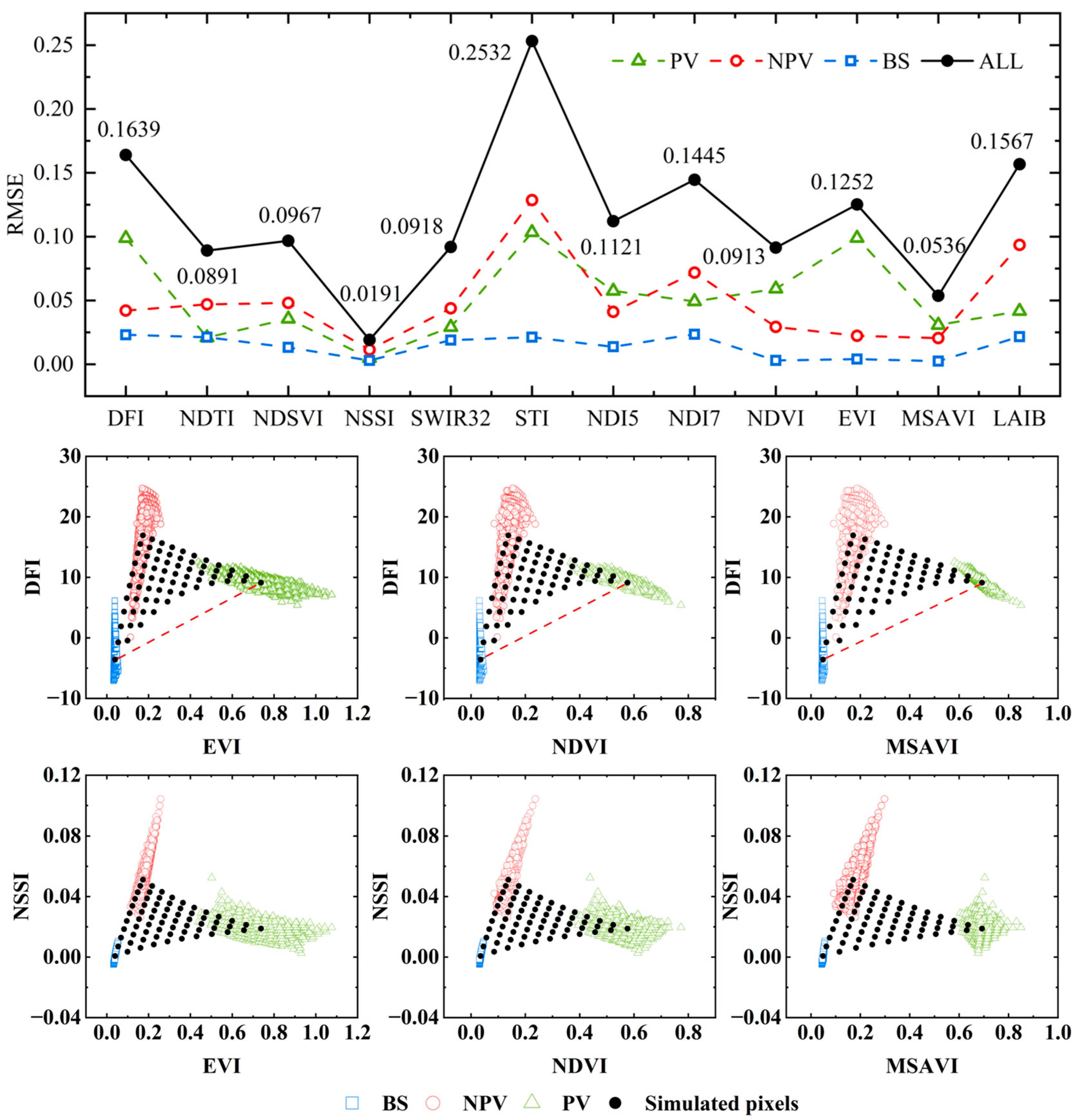
We compared the baseline endmember values with the discrete endmember values using the preprocessed spectral dataset. Taking Sentinel-2A data as an example, cross regional differences in vegetation indices were calculated. Furthermore, a feature space was constructed based on the NPV and PV index, with the results presented in Figure 17. Among the pure endmember values, the STI endmember value has the highest RMSE and the lowest stability, while the NSSI endmember value has the lowest RMSE and the highest stability. In the PV indices, the LAIB endmember value RMSE is the highest and the stability is the lowest, while the MSAVI endmember value RMSE is 0.0536 and the stability is the highest. The high stability of the endmember values indicates that the model is insensitive to vegetation types and regional changes in large-scale estimation.

The scattered points in Figure 17 are the distribution areas of endmember values collected in different areas, and the endmember values with the lowest error are selected through stability analysis to construct the feature space. The triangular feature space by DFI failed to effectively construct a typical triangular feature space. The simulated pixel points are concentrated at the bottom, especially in the intersection area between non photosynthetic vegetation and bare land. The triangle is concave inward, and the internal image element points are arranged tightly, which may lead to high overlap of pixel points and result in misclassification when inverting bare land and non-photosynthetic vegetation. On the contrary, the triangular feature space formed by the NSSI has a more uniform distribution of image elements and the smallest difference from the endmember values.

During inversion, when the target study area is a dense green vegetation zone, pixels of remote sensing images will be distributed in the green pixel region shown in Figure 17; when the target study area is a withered vegetation zone, the pixels will be distributed in the red pixel region; and when the target study area is large-scale bare land, the target pixels will be distributed in the blue pixel region. Significant deviations may occur when extracting endmember values, so measured endmember values should be used instead of remote sensing-derived endmember values. In indices such as EVI, MSAVI, and NDVI, the dominant relationship is PV > NPV > BS; in NSSI and DFI, the dominant relationship is NPV > PV > BS, which is consistent with the assumption of the ternary linear mixed model and verifies its application as a parameter selection for inversion modeling.

Comparative identification and analysis were performed for the oasis and desert regions using both traditional and optimized models (Figure 11). The coverage information estimated before and after optimization is presented in

Table 11. The coverage of Qingtu Lake estimated before and after optimization.

PVI	NPVI	NO.	fNPV	fPV	fBS
NDVI	NSSI	D.	39.94%	19.12%	40.94%
		E.	61.55%	20.12%	18.33%
EVI	NSSI	F.	38.75%	13.47%	47.78%
		G.	61.02%	18.94%	20.04%
MSAVI	NSSI	H.	40.08%	18.75%	41.17%
		I.	61.42%	21.12%	17.46%

PVI refers to PV Index, and NPVI refers to NPV Index.

. Field verification confirmed that the central transect represents a bare soil-covered roadway, which should be classified as BS in inversion results. The traditional model’s decomposition exhibited significant misclassification: road sections were consistently misidentified as NPV across all parameter sets, with additional erroneous NPV classification occurring in vegetated areas where bare soil patches were present, resulting in mixed NPV pixels. The estimated NPV coverage before optimization was approximately 20% higher than that after optimization across various parameters, indicating a substantial overestimation and misidentification phenomenon prior to the optimization process. In contrast, the optimized model correctly identified bare soil features while demonstrating enhanced spectral discrimination between NPV and bare soil. This systematic misclassification by the traditional model was corroborated by consistent error patterns observed across different vegetation indices in Figure 18, aligning with the feature space distributions presented in Figure 17.

4.3. Spatial Block Validation of Model Performance

In relevant studies, the validation method used involves global fitting verification between measured data and inverted data. However, spatial autocorrelation exists in remote sensing, which can lead to overestimation in validation results [34]. Therefore, based on the spatial sampling method proposed by Bahn [35], the accuracy of the model inversion was re-evaluated. The validation points were divided into five regions according to their regional characteristics during data collection: River, Oasis, Desert, Urban, and Mixed. Spatial block validation was then conducted again based on the optimal parameters. The validation results are shown in

Table 12. Comparison of model accuracy evaluation results.

Method	Validation Area	R2	RMSE
Global validation	All	0.7825 **	0.0232
Spatial block validation	Average	0.7017 **	0.0279
	River	0.6535 **	0.0287
	Oasis	0.7845 **	0.0212
	Desert	0.8031 **	0.0194
	Urban	0.5373 **	0.0376
	Mixed	0.7299 **	0.0324

Regression analysis, ** p < 0.01.

.

As can be seen from Table 12, the spatial block validation results show decreases in both R² and RMSE compared to the global validation results, but they still represent good validation outcomes. Due to the influence of various anthropogenic factors in urban areas and the impact of moisture in river areas, the validation results for these two regions declined. However, the validation results for the oasis, desert, and mixed regions remained good. Future research could focus on further optimization for urban and river areas.

While the spatial block validation implemented here provides a more robust evaluation, it also highlights a fundamental challenge: the spatial dependence inherent in remote sensing data can lead to inflated correlations in driver analyses. To unequivocally disentangle true functional relationships from spurious spatial correlations in future work, the application of spatially explicit statistical models is essential. This approach will allow for a more rigorous identification of the underlying environmental and anthropogenic drivers governing NPV dynamics.

4.4. Necessity of PV Indices Further Examination

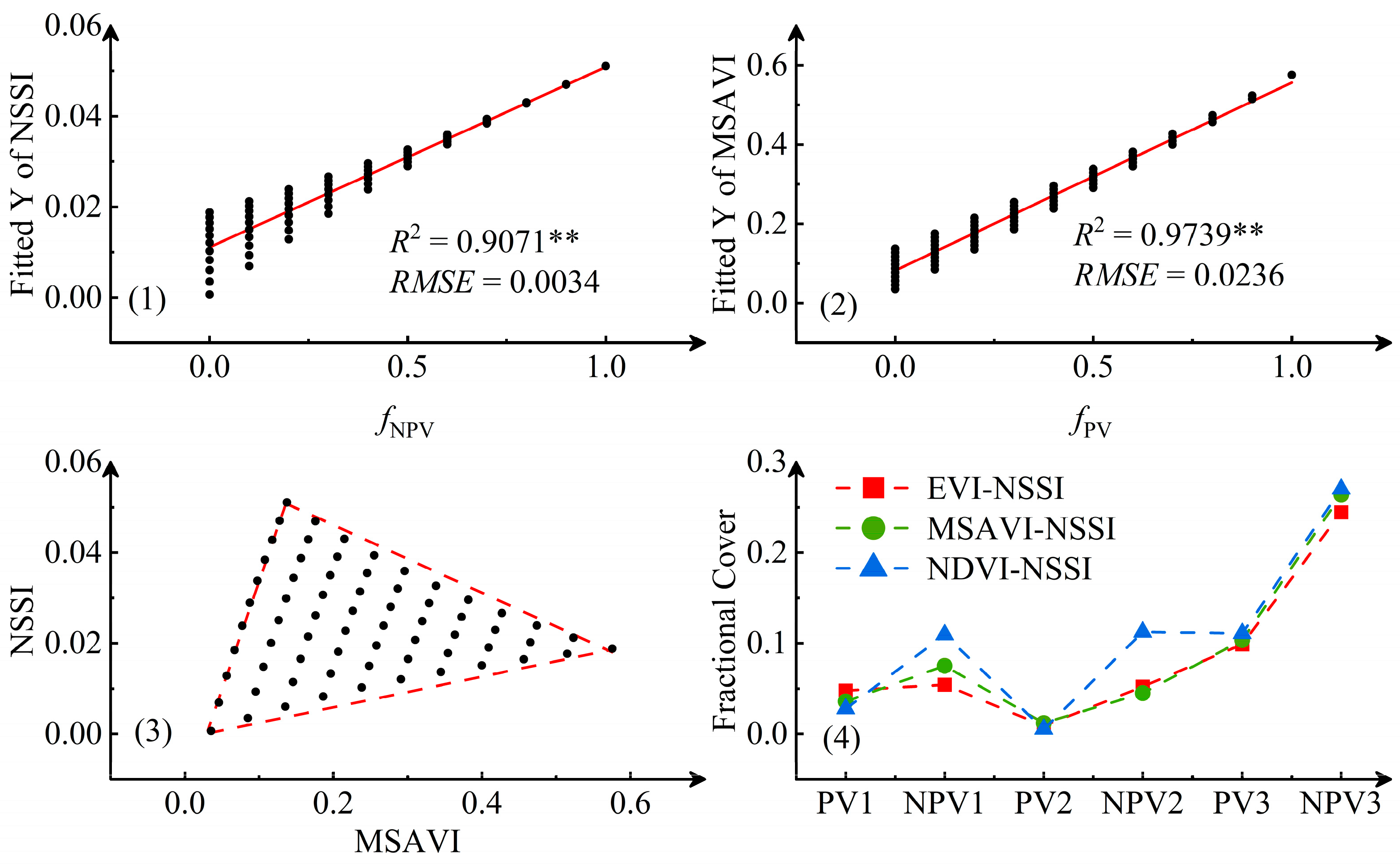
For the optimized NPV identification model in arid regions with sparse vegetation, the MSAVI and NSSI were selected for spectral inversion. As shown in Figure 19, MSAVI and NSSI demonstrated superior performance in the validation assessment of the spectral dataset. The feature space constructed by MSAVI and NSSI exhibited uniform pixel distribution, with MSAVI showing a significant positive correlation with photosynthetic vegetation fraction cover, indicating its enhanced potential for discriminating among the three target land cover types. Previous studies primarily evaluated linear regression results between NPV indices and coverage. However, following NPV index analysis, further examination of PV indices is essential. Figure 19(4) illustrates discrepancies between inversion results and ground truth values across parameters in the Qintu lake region. When NSSI was designated as the NPV index, inversion results using EVI, MSAVI, and NDVI to construct distinct feature spaces revealed significant variations. Consequently, the critical role of photosynthetic vegetation indices cannot be overlooked during index optimization and selection.

Many previous studies directly utilized the NDVI as the inversion index for calculations. Among them, Song used the NDVI-DFI to verify the calculation in the study of Junggar Basin [9]. Hou used the NDVI-DFI for the inversion of NPV in the analysis of the surface thermal environment differentiation effect of the intensive mining development area [8]; Zhu proposed that since the NDVI was easily saturated in environments with dense vegetation growth, such as forested areas, the EVI was used to allow the saturation problem to be alleviated by replacing the NDVI with the EVI [3]. Experimental evidence has shown that NDVI is sensitive to changes in the soil background and is influenced by either excessively high or low vegetation fractional cover. When vegetation fractional cover exceeds 80%, the NDVI becomes saturated and its sensitivity decreases; the NDVI value is too high below 25% vegetation fractional cover.

Additionally, spectral datasets constructed from field-measured spectra are critically important for model optimization. Under data-limited conditions, a step size of 0.1 is typically applied, whereas a 0.2 step size is predominantly utilized when handling diverse vegetation types in data-rich scenarios. Whether higher-precision step sizes (e.g., 0.05 or 0.02) in dataset construction can yield improved model evaluation results remains an open research question requiring further investigation.

Furthermore, it was observed that due to the inherent genetic and spectral coupling between soil organic matter (SOM) and NPV, spectral confusion exists, which represents an inherent challenge in optical remote sensing unmixing [36,37]. Therefore, the endmember spectra used in this study reflect macroscopic spectral characteristics under natural conditions rather than attempting to explicitly separate organically influenced soil components. Future work should prioritize the construction of a more refined spectral library based on pure crop residues and soils at different decomposition stages, combined with multi-temporal data to better decouple these spectrally entangled signals.

5. Conclusions

The objective of this study is to optimize traditional NPV cover inversion models while conducting vegetation index selection analysis and refining inversion indices for different sensors. Optimization is achieved through multi-source remote sensing data fusion, enhancing spatial heterogeneity representation in the traditional model. The main conclusions drawn from this study are as follows:

(1)

The incorporation of spatial heterogeneity analysis and additional field spectral matrix information into the traditional model significantly improved inversion accuracy by better aligning with actual conditions. The optimized model demonstrated enhanced performance with an R² of 0.7825 and RMSE of 0.0232, confirming the effectiveness of the model optimization. Compared to traditional spectral mixture analysis models, the incorporation of spatial heterogeneity analysis significantly enhances NPV detection accuracy, providing guidance for ecological health assessments under climate change in arid and semi-arid area.

(2)

Vegetation indices exhibit sensor-dependent performance variations due to spectral band differences. For Sentinel-2, the MSAVI and NSSI demonstrated optimal fitting with f_NPV, achieving R² values of 0.9739 and 0.9071, respectively, within the spectral dataset. In contrast, Landsat 8 and MODIS sensors showed improved performance when combining MSAVI with the optimized vegetation index DFIEXP, attributable to their respective band limitations.

(3)

By optimizing the spectral constraint weights of endmembers in remote sensing imagery, NPV can be more effectively identified across various phenological conditions, providing a solution for long-term vegetation health monitoring.

References

1. Verrelst, J.; Halabuk, A.; Atzberger, C.; Hank, T.; Steinhauser, S.; Berger, K. A comprehensive survey on quantifying non-photosynthetic vegetation cover and biomass from imaging spectroscopy. Ecol. Indic. 2023, 155, 110911. [Google Scholar] [CrossRef]
2. Guerschman, J.P.; Hill, M.J.; Renzullo, L.J.; Barrett, D.J.; Marks, A.S.; Botha, E.J. Estimating fractional cover of photosynthetic vegetation, non-photosynthetic vegetation and bare soil in the australian tropical savanna region upscaling the EO-1 hyperion and MODIS sensors. Remote Sens. Environ. 2009, 113, 928–945. [Google Scholar] [CrossRef]
3. Zhu, C.; Tian, J.; Tian, Q.; Wang, X.; Li, Q. Using NDVI-NSSI feature space for simultaneous estimation of fractional cover of non-photosynthetic vegetation and photosynthetic vegetation. Int. J. Appl. Earth Obs. Geoinf. 2023, 118, 103282. [Google Scholar] [CrossRef]
4. Jiapaer, G.; Chen, X.; Bao, A. A comparison of methods for estimating fractional vegetation cover in arid regions. Agric. For. Meteorol. 2011, 151, 1698–1710. [Google Scholar] [CrossRef]
5. Byambakhuu, I.; Sugita, M.; Matsushima, D. Spectral unmixing model to assess land cover fractions in Mongolian steppe regions. Remote Sens. Environ. 2010, 114, 2361–2372. [Google Scholar] [CrossRef]
6. Mishra, N.B.; Crews, K.A. Estimating fractional land cover in semi-arid central Kalahari: The impact of mapping method (spectral unmixing vs. object-based image analysis) and vegetation morphology. Geocarto Int. 2014, 29, 860–877. [Google Scholar] [CrossRef]
7. Zheng, B.; Campbell, J.B.; Serbin, G.; Daughtry, C.S.T. Multitemporal remote sensing of crop residue cover and tillage practices: A validation of the minNDTI strategy in the United States. J. Soil Water Conserv. 2013, 68, 120–131. [Google Scholar] [CrossRef]
8. Hou, C.H.; Li, F.P.; Feng, Y.F.; Gu, H.H.; Yuan, X.T.; Song, W.; Liu, H.X. Analysis of differentiation effect of sur-face thermal environment in intensive mining areas based on NDVI-DFI model. Trans. Chin. Soc. Agric. Eng. 2020, 36, 160–168. [Google Scholar] [CrossRef]
9. Song, J.; Xia, N.; Hai, W.; Tang, M.Y. Spatial-temporal variation of vegetation in Gobi region of Xinjiang based on NDVI-DFI model. Southwest China J. Agric. Sci. 2022, 35, 2867–2875. [Google Scholar] [CrossRef]
10. Tang, M.Y.; Ding, J.L.; Xia, N.; Zhang, Z. Estimation of vegetation in the Boertala mongolian autonomy prefecture based on NDVI-DFI mode. Sci. Surv. Mapp. 2019, 44, 74–81. [Google Scholar] [CrossRef]
11. Bai, X.L. Relationship of reflectance spectral and fractional cover of various non-photosynthetic vegetation. Acta Ecol. Sin. 2022, 42, 186–195. [Google Scholar] [CrossRef]
12. Chai, G.Q.; Wang, J.P.; Wang, G.Z.; Kang, L.; Wu, M.; Wang, Z. Estimation of fractional cover of non-photosynthetic vegetation in typical steppe based on MODIS data. Remote Sens. Land Resour. 2018, 31, 2836–2844. [Google Scholar] [CrossRef]
13. Delegido, J.; Verrelst, J.; Rivera, J.P.; Ruiz-Verdú, A.; Moreno, J. Brown and green LAI mapping through spectral indices. Int. J. Appl. Earth Obs. Geoinf. 2015, 35, 350–358. [Google Scholar] [CrossRef]
14. Wang, G.Z.; Wang, J.P.; Zou, X.Y.; Wang, Z.L.; Zong, M. Estimation of fractional cover of photosynthetic and non-photosynthetic vegetation in the xilingol steppe region using the NDVI-DFI model. Acta Ecol. Sin. 2017, 37, 5722–5731. [Google Scholar] [CrossRef]
15. Luo, Y.X.; Ji, C.C.; Li, X.S.; Xu, J.H. Vegetation Index Model for Estimating Sparse Photosynthetic/ Non-photosynthetic Vegetation Fractional Cover in Arid Zone. Remote Sens. Inf. 2022, 37, 57–64. [Google Scholar] [CrossRef]
16. Xu, M.Z.; Xu, H.; Kong, P.; Wu, Y.L. Remote Sensing Vegetation Classification Method Based on Vegetation Index and Convolution Neural Network. Laser Optoelectron. Prog. 2022, 59, 2428005. [Google Scholar] [CrossRef]
17. Han, X. Resaerch data: Measured hyperspectral data of vegetation and soil in northwest China. Mendeley Data 2025. [Google Scholar] [CrossRef]
18. Ji, C.; Jia, Y.; Gao, Z.; Wei, H.; Li, X. Nonlinear spectral mixture effects for photosynthetic/non-photosynthetic vegetation cover estimates of typical desert vegetation in western china. PLoS ONE 2017, 12, e0189292. [Google Scholar] [CrossRef]
19. Yuan, H.; Ji, C.C.; Yang, X.M.; Chen, M.L.; Pan, J.P.; Cao, Y.M. Construction of sparse non-photosynthetic vegetation index combining sentinel-2 data and spectral features. J. Geo-Inf. Sci. 2023, 25, 1894–1907. [Google Scholar] [CrossRef]
20. Wang, G.; Wang, J.; Zou, X.; Chai, G.; Wu, M.; Wang, Z. Estimating the fractional cover of photosynthetic vegetation, non-photosynthetic vegetation and bare soil from MODIS data: Assessing the applicability of the NDVI-DFI model in the typical xilingol grasslands. Int. J. Appl. Earth Obs. Geoinf. 2019, 76, 154–166. [Google Scholar] [CrossRef]
21. Tucker, C.J. Red and photographic infrared linear combinations for monitoring vegetation. Remote Sens. Environ. 1979, 8, 127–150. [Google Scholar] [CrossRef]
22. Huete, A.; Didan, K.; Miura, T.; Rodriguez, E.P.; Gao, X.; Ferreira, L.G. Overview of the radiometric and biophysical performance of the MODIS vegetation indices. Remote Sens. Environ. 2002, 83, 195–213. [Google Scholar] [CrossRef]
23. Qi, J.; Chehbouni, A.; Huete, A.R.; Kerr, Y.H.; Sorooshian, S. A modified soil adjusted vegetation index. Remote Sens. Environ. 1994, 48, 119–126. [Google Scholar] [CrossRef]
24. van Deventer, A.P.; Ward, A.D.; Gowda, P.H.; Lyon, J.G. Using Thematic Mapper Data to Identify Contrasting Soil Plains and Tillage Practices. Photogramm. Eng. Remote Sens. 1997, 63, 87–93. [Google Scholar]
25. Jacques, D.C.; Kergoat, L.; Hiernaux, P.; Mougin, E.; Defourny, P. Monitoring dry vegetation masses in semi-arid areas with MODIS SWIR bands. Remote Sens. Environ. 2014, 153, 40–49. [Google Scholar] [CrossRef]
26. Cao, X.; Chen, J.; Matsushita, B.; Imura, H. Developing a MODIS-based index to discriminate dead fuel from photosynthetic vegetation and soil background in the Asian steppe area. Int. J. Remote Sens. 2010, 31, 1589–1604. [Google Scholar] [CrossRef]
27. Tian, J.; Su, S.; Tian, Q.; Zhan, W.; Xi, Y.; Wang, N. A novel spectral index for estimating fractional cover of non-photosynthetic vegetation using near-infrared bands of sentinel satellite. Int. J. Appl. Earth Obs. Geoinf. 2021, 101, 102361. [Google Scholar] [CrossRef]
28. Qi, J.; Marsett, R.; Heilman, P.; Bieden-Bender, S.; Moran, S.; Goodrich, D.; Weltz, M. RANGES improves satellite-based information and land cover assessments in southwest United States. EoS Trans. 2002, 83, 601–606. [Google Scholar] [CrossRef]
29. Wang, G.; Wang, J.; Han, L.; Chai, G.; Wang, Z. Estimation of Non-Photosynthetic Vegetation Coverage Using Simulated Landsat-8 OLI Data Based on Measured Spectra. J. Geo-Inf. Sci. 2018, 20, 1667–1678. [Google Scholar]
30. Asner, G.P.; Heidebrecht, K.B. Spectral unmixing of vegetation, soil and dry carbon cover in arid regions: Comparing multispectral and hyperspectral observations. Int. J. Remote Sens. 2002, 23, 3939–3958. [Google Scholar] [CrossRef]
31. Chai, G. Estimation of Non-Photosynthetic Vegetation Coverage and Its Spatiotemporal Variations in Xilingol Grassland Based on MODIS Data. Master’s Thesis, Ludong University, Yantai, China, 2021. [Google Scholar]
32. Kokaly, R.F.; Clark, R.N.; Swayze, G.A.; Livo, K.E.; Hoefen, T.M.; Pearson, N.C.; Wise, R.A.; Benzel, W.M.; Lowers, H.A.; Driscoll, R.L.; et al. USGS Spectral Library Version 7 Data: U.S. Geological Survey Data Release; USGS: Reston, VA, USA, 2017. [Google Scholar] [CrossRef]
33. Boardman, J.W.; Kruse, F.A.; Green, R.O. Mapping Target Signatures via Partial Unmixing of AVIRIS Data (Report No. N95-33); Jet Propulsion Laboratory, California Institute of Technology: Pasadena, CA, USA, 1995. [Google Scholar]
34. Ploton, P.; Mortier, F.; Réjou-Méchain, M.; Barbier, N.; Picard, N.; Rossi, V.; Dormann, C.; Cornu, G.; Viennois, G.; Bayol, N.; et al. Spatial validation reveals poor predictive performance of large-scale ecological mapping models. Nat. Commun. 2020, 11, 4540. [Google Scholar] [CrossRef]
35. Bahn, V.; McGill, B.J. Testing the predictive performance of distribution models. Oikos 2012, 122, 321–331. [Google Scholar] [CrossRef]
36. Lehmann, J.; Kleber, M. The contentious nature of soil organic matter. Nature 2015, 528, 60–68. [Google Scholar] [CrossRef]
37. Ji, W.J.; Shi, Z.; Zhou, Q.; Zhou, L.Q. VIS-NIR reflectance spectroscopy of the organic matter in several types of soils: VIS-NIR reflectance spectroscopy of the organic matter in several types of soils. J. Infrared Millim. Waves 2012, 31, 277–282. [Google Scholar] [CrossRef]
Figure 1. Structure of research data.
Remotesensing 17 03480 g001
Figure 2. Composite spectral transmission curve and channel information of UAV.
Remotesensing 17 03480 g002
Figure 3. Classification of UAV data: red was classified as non-photosynthetic vegetation, green was classified as photosynthetic vegetation, and yellow was classified as bare soil.
Remotesensing 17 03480 g003
Figure 4. Hyperspectral curves of PV, NPV, BS, and mean values.
Remotesensing 17 03480 g004
Figure 5. Spatial distribution maps of measured spectral data under NDVI-DFI indices and field survey maps.
Remotesensing 17 03480 g005
Figure 6. The band characteristics of hyperspectral information following convolution with the spectral convolution functions of Sentinel-2, MOD09GA, and Landsat8.
Remotesensing 17 03480 g006
Figure 7. Comparison of validation between original and optimized indices.
Remotesensing 17 03480 g007
Figure 8. Validation and comparison of inversion results.
Remotesensing 17 03480 g008
Figure 9. Raster map comparison of inversion results.
Remotesensing 17 03480 g009
Figure 10. Results of validation of UAV data and remote sensing data.
Remotesensing 17 03480 g010
Figure 11. Results of fitting UAV data and remote sensing data.
Remotesensing 17 03480 g011
Figure 12. Sentinel-2A: Classification inversion results and fractional cover inversion results: (A) is the Junggar Basin region, (B) is the East Juyan lake, (C) is the Qintu lake.
Remotesensing 17 03480 g012
Figure 13. Landsat8: Fractional cover inversion results in East Juyan Lake.
Remotesensing 17 03480 g013
Figure 14. MOD09GA: Classification inversion results and fractional cover inversion results in China.
Remotesensing 17 03480 g014
Figure 15. Changes in spectral endmember values under the MODIS sensor.
Remotesensing 17 03480 g015
Figure 16. Spectral curves of PV, NPV, and BS in arid, grassland, and forest regions, as well as band-wise line charts after hyperspectral convolution with sensors. In the convolved images, the long dashed line represents PV, the short dotted line represents BS, and the solid line represents NPV.
Remotesensing 17 03480 g016
Figure 17. Results of the endmember values.
Remotesensing 17 03480 g017
Figure 18. (A). True-color remote sensing image of Qintu Lake, with the red box as the comparison area; (B). True-color remote sensing image of a selected small area; (C). False-color remote sensing image; (D,F,H) display the inversion results from the optimized model using NDVI, EVI, and MSAVI as parameters, respectively, whereas (E,G,I) present results with the conventional model. Red represents NPV, green represents PV, and blue represents BS.
Remotesensing 17 03480 g018
Figure 19. (1) Linear regression plot of MSAVI versus PV fractional cover under the simulated dataset, (2) linear regression plot of NSSI versus NPV fractional cover, (3) MSAVI-NSSI space under the simulated dataset, (4) different results with different PV indices.
Remotesensing 17 03480 g019