Angle-Controllable SAR Image Generation and Target Recognition via StyleGAN2

Highlights

What are the main findings?

• Conditional StyleGAN2 generates high-quality, angle-controllable SAR images.
• Recognition accuracy improves by 6.03% on self-constructed and 7.14% on SAMPLE dataset.

What is the implication of the main finding?

• Angle encoder and attention modules enhance image fidelity and generalization.
• The framework provides an effective solution for multi-view SAR image generation and recognition.

Abstract

Due to the inherent characteristics of synthetic aperture radar (SAR) imaging, variations in target orientation, and the challenges posed by non-cooperative targets (i.e., targets without cooperative transponders or external markers), limited viewpoint coverage results in a small-sample problem that severely constrains the application of deep learning to SAR image interpretation and target recognition. To address this issue, this paper proposes a multi-target, multi-view SAR image generation method based on conditional information and StyleGAN2, designed to generate high-quality, angle-controllable SAR images of typical targets from limited samples. The proposed framework consists of an angle encoder, a generator, and a discriminator. The angle encoder employs a sinusoidal encoding scheme that combines sine and cosine functions to address the discontinuity inherent in one-hot angle encoding, thereby enabling precise angle control. Moreover, the integration of SimAM and IAAM attention mechanisms enhances image quality, facilitates accurate angle control, and improves the network’s generalization to untrained angles. Experiments conducted on a self-constructed dataset of typical civilian targets and the SAMPLE subset of the MSTAR dataset demonstrate that the proposed method outperforms existing baselines in terms of structural fidelity and feature distribution consistency. The generated images achieve a minimum FID of 6.541 and a maximum MS-SSIM of 0.907, while target recognition accuracy improves by 6.03% and 7.14%, respectively. These results validate the feasibility and effectiveness of the proposed approach for SAR image generation and target recognition tasks.

1. Introduction

As one of the crucial imaging methods in remote sensing, surveying and mapping, reconnaissance, and other fields, synthetic aperture radar has also been playing an important role in military and civilian fields [1,2]. With the continuous development of deep learning technology, research methods for understanding and interpreting SAR images are in urgent need of new progress [3,4]. However, deep learning-based research methods generally require sufficient labeled data. Unfortunately, existing datasets are still very limited, and publicly available large-scale SAR image datasets are extremely scarce. Most current algorithms are based on limited public SAR image datasets such as MSTAR [5]. SAR image datasets are still expensive and difficult to obtain. This is especially difficult for non-cooperative targets, as obtaining target sample SAR images with multi-angle information is even more challenging. This limits the application of deep learning technology to SAR imagery and hinders the development of fields that include, but are not limited to, multi-target classification and detection [6,7,8,9], multi-target SAR automatic recognition [10,11], and multi-sensor SAR image fusion [12]. In particular, the small sample problem arises from insufficient view coverage due to factors such as satellite orbit constraints and the orientation of typical target scenes [13,14,15]. In addition to deep learning methods, traditional machine-learning classifiers such as Support Vector Machines (SVM) and Random Forests (RF) remain widely used in SAR ATR under limited-data regimes, especially when hand-crafted radiometric or texture features (e.g., ${\sigma }^0$, ${\gamma }^0$, ${\beta }^0$, GLCM, LBP) are available. These shallow classifiers are computationally efficient and often competitive for classification, but being discriminative rather than generative they cannot by themselves provide controllable multi-azimuth sample synthesis required for data augmentation of deep end-to-end ATR models [16].

Traditional small sample enhancement methods include translation, shearing, rotation, scaling, adding noise, etc. [17]. However, this method only changes the shape of the image at the geometric level, which is suitable for optical image amplification. It does not consider the imaging mechanism and special imaging geometry of SAR images [18]. It cannot change based on changes in pitch and azimuth angles, and it is difficult to reflect the sensitivity of SAR target samples to changes in physical characteristics [19,20]. Therefore, it is not effective in SAR image applications and cannot achieve controllable data enhancement at specific angles. However, for SAR image target recognition and detection, observing the target from multiple angles, particularly from various azimuths, can provide richer features that enhance recognition accuracy [21]. Therefore, how to combine the special mechanism of SAR images to complete multi-view image amplification and improve target recognition accuracy is a top priority in current research. Moreover, standard SAR radiometric normalizations—commonly referred to as beta-nought (${\beta }^0$), sigma-nought (${\sigma }^0$) and gamma-nought (${\gamma }^0$)—represent backscatter normalized with respect to different reference areas and are routinely used for radiometric calibration and terrain correction in SAR processing. Such physics-based corrections and derived radiometric features can improve target discrimination, but they typically rely on accurate imaging geometry and calibration parameters and therefore are not straightforward to generalise for continuous, azimuth-controllable sample synthesis across diverse multi-target datasets [22].

Existing multiview augmentation strategies for SAR imaging primarily include electromagnetic modeling and simulation, as well as deep learning-based approaches. Although high-precision SAR samples can be generated via electromagnetic computations, SAR echo simulation, and imaging simulation, deep learning models typically require tens of thousands to hundreds of thousands of samples for effective training. Given current computational resources and technological constraints, generating the entire dataset solely through these methods is highly time-consuming and, in some cases, infeasible [23]. A practical solution involves producing a moderate number of high-fidelity samples derived from accurate electromagnetic calculations and SAR echo simulations while ensuring sample balance and comprehensive parameter coverage. Leveraging these high-fidelity samples in conjunction with physical feature guidance, an efficient sample augmentation method can be employed to construct large-scale datasets, thereby mitigating model overfitting and enhancing generalisation and robustness.

Current generative adversarial networks (GANs) have been widely applied to SAR image augmentation. For example, Song et al. [24] proposed an adversarial autoencoder (AAE) for SAR representation and synthesis, showing that, from only 90 training samples with azimuth separations of at least 25°, a large set of previously unseen viewing angles (1748 samples) can be synthesized. Zhang et al. [25] extended DCGAN by incorporating an azimuth discriminator to generate SAR images at specified azimuths. Cui et al. [26] adopted WGAN-GP and cascaded a pretrained SVM classifier as an image filter, improving sample quality by selecting azimuth-consistent outputs. Wang et al. [27] used SAGAN to perform azimuthal interpolation for multi-view SAR targets, offering a practical approach for dataset expansion. Zeng et al. [28] proposed an angle-transformation GAN (ATGAN) that models inter-azimuth feature mappings in a spatial-transformation layer, enabling high-precision azimuth-controllable synthesis.

These studies collectively demonstrate that GANs substantially advance azimuth-controllable SAR synthesis. Meanwhile, diffusion models have recently been explored for SAR image generation; for instance, Qosja et al. applied denoising diffusion probabilistic models (DDPMs) to SAR synthesis. Although diffusion models often yield superior sample fidelity, their sampling typically requires tens to hundreds of iterative steps, resulting in substantially higher inference cost and reduced suitability for ATR data-augmentation pipelines that demand rapid bulk synthesis. Moreover, SAR datasets are frequently small-scale, and GANs endowed with suitable priors (e.g., StyleGAN2 [29]) can more rapidly learn target statistics from limited data while providing an explicit, manipulable latent space. Prior work has also shown that GAN-based augmentation can enhance the interpretability of SAR ATR models.

Therefore, when considering the combined requirements of controllability and generation efficiency, GANs retain practical advantages. In this work, we propose a multi-target, multi-azimuth SAR synthesis method that integrates StyleGAN2 with an explicit angle encoder. Compared with previous approaches that rely on conditional modules or local fusion mechanisms for azimuth interpolation, our method leverages StyleGAN2’s latent-space modeling and injects an explicit angle code (latent conditioning + explicit angle injection) to achieve fine-grained azimuth control while preserving style characteristics. Concretely, we first construct high-fidelity multi-target datasets via electromagnetic modeling [30] and SAR echo simulation [31], then combine StyleGAN2 with an angle encoder to produce high-quality azimuthal interpolation for multiple targets—providing a new avenue for small-sample augmentation and multi-azimuth dataset construction. Finally, we validate the quality and controllability of the generated images using several objective evaluation metrics. The main contributions of this paper are as follows:

1.

We propose a hybrid SAR data-augmentation strategy that combines electromagnetic simulation with deep generative modeling to efficiently produce multi-view samples for few-shot scenarios.

2.

We introduce a controllable StyleGAN2-based architecture augmented with an explicit angle encoder, enabling fine-grained azimuth interpolation in the latent space.

3.

We validate the proposed approach using multiple objective metrics and downstream recognition tasks, demonstrating improved fidelity and angle controllability compared with existing augmentation strategies.

2. Selection and Construction of Multi-Target Datasets

2.1. Multi-Target Selection and Detailed Modeling

Currently, research on GAN-based SAR image generation predominantly revolves around the MSTAR dataset. To tackle the challenge of limited diversity in multi-angle synthetic aperture radar (SAR) image datasets for typical civilian targets, and considering the wide-ranging applications of SAR in both military and civilian contexts, this paper develops a dataset that includes 15 common and representative targets from civilian domains. These include ground targets, maritime targets, and aerial targets. The dimensions and categories of typical targets are shown in

Table 1. Dimensions and categories of the fifteen typical targets used in the experiments.

Target	Length (m)	Category
Fire Truck	13.4	Ground
Heavy Truck	9.32	Ground
Bus	12.2	Ground
Tram (single car)	13.5	Ground
Airstairs	12.0	Ground
Coal Mining Truck	11.25	Ground
Radar Car	9.6	Ground
Barge	150.0	Maritime
Container Ship	365.0	Maritime
Oil Tanker	280.0	Maritime
Dredger 4017	103.0	Maritime
Sand Barge	80.0	Maritime
Piaggio P180	14.4	Aerial
Bell 412 helicopter	17.1	Aerial
Glider	7.85	Aerial

.

Subsequently, geometric modeling was conducted for the 15 selected typical targets using scaled-down models. Stepwise precision-controlled mapping techniques were employed to perform accurate measurements and high-fidelity reverse 3D modeling of these reduced-scale targets [32,33]. In comparison to conventional 3D geometric reconstruction approaches, the scaled-model-based method provides several advantages, including adaptable dimensions, high controllability, efficient data storage and processing, and strong interpretability.

Since actual targets or scenes are often large in size, while synthetic aperture radar (SAR) imaging simulations are typically constrained by computational resources and processing time, the use of scaled models enables size reduction to meet the practical requirements of such experiments. This approach significantly simplifies subsequent calculations and processing [34]. Moreover, scaling facilitates the adjustment of target dimensions to accommodate various simulation scenarios.

The detailed modeling workflow consists of three main stages: (1) data acquisition; (2) data preprocessing; (3) surface reconstruction. Data acquisition involves capturing geometric information of the target using specialized instruments; data preprocessing converts this information into 3D coordinates, shape, texture, and other relevant descriptors; surface reconstruction entails combining multiple modeling techniques according to the physical characteristics of the target and the requirements of the simulation scenario to generate the desired 3D model. Throughout this process, 3D model files in the .3ds format (a common format for storing 3D mesh data) and scene description files in the .pov format (used by the POV-Ray ray-tracing software) were produced for each typical target. Figure 1 presents optical images of all targets alongside their corresponding 3D models.

2.2. Multi-Target Electromagnetic Modeling and Echo Simulation

In order to construct a multi-angle dataset of typical civilian targets, this study employs electromagnetic scattering modelling for 15 representative targets. The electromagnetic scattering computations utilise a ray-tracing method [35] based on the Phong shading optical model to determine the three-dimensional coordinates of target scattering points. This is combined with the physical optics (PO) method to compute the scattering intensity of these points [36,37]. Together, these approaches enable efficient calculation of both the spatial coordinates and intensities of scattering points within a three-dimensional coordinate system (range, azimuth, and elevation). The physical optics method, also referred to as the Kirchhoff approximation under scalar assumptions, is applied to handle slightly rough surfaces that satisfy the following conditions [38]:

$$kl>6,l^2>2.76s\lambda ,m<0.25$$

(1)

where $k={\displaystyle \frac{2\pi }{\lambda }}$ is the wavenumber (rad m⁻¹) corresponding to the radar wavelength $\lambda$ (m); l is the surface correlation length representing the horizontal roughness scale (m); s is the root-mean-square (RMS) surface height (m); and $m=s/l$ is the surface slope parameter (dimensionless). These conditions ensure that the physical optics (PO) approximation, also known as the Kirchhoff approximation, is valid for slightly rough surfaces. The incoherent backscatter coefficient for pp polarisation is given by [39]:

$${\sigma }_{pp}^{\circ }\left(\theta \right)=k^2{\cos }^2\theta ·{\mathrm{\Gamma }}_p\left(\theta \right)\exp \left[-{\left(2ks\cos \theta \right)}^2\right]\sum _{n=1}^{\infty }{\displaystyle \frac{{\left(2ks\cos \theta \right)}^{2n}}{n!}}·I$$

(2)

where ${\sigma }_{pp}^{\circ }\left(\theta \right)$ denotes the normalized radar cross-section (NRCS) for $pp$-polarization; ${\mathrm{\Gamma }}_p\left(\theta \right)$ is the Fresnel reflectivity for p-polarization ($p=v$ or h); $\theta$ is the local incidence angle; and I represents the integral term derived from the surface autocorrelation function (not the image intensity used in SAR backscattering computation). For the surface of the Gaussian autocorrelation function,

$$I={\displaystyle \frac{l^2}{n}}\exp \left[-{\displaystyle \frac{{\left(kl\sin \theta \right)}^2}{n}}\right]$$

(3)

where n is a roughness-related integer parameter introduced in the series expansion of the incoherent term; l is the surface correlation length; and $\theta$ is the local incidence angle. For the exponential autocorrelation function,

$$I={\displaystyle \frac{n{l}^2}{{\left[n^2+2{\left(kl\sin \theta \right)}^2\right]}^{3/2}}}$$

(4)

where k is the wavenumber; l is the surface correlation length; n is the roughness-related integer parameter; and $\theta$ is the incidence angle.

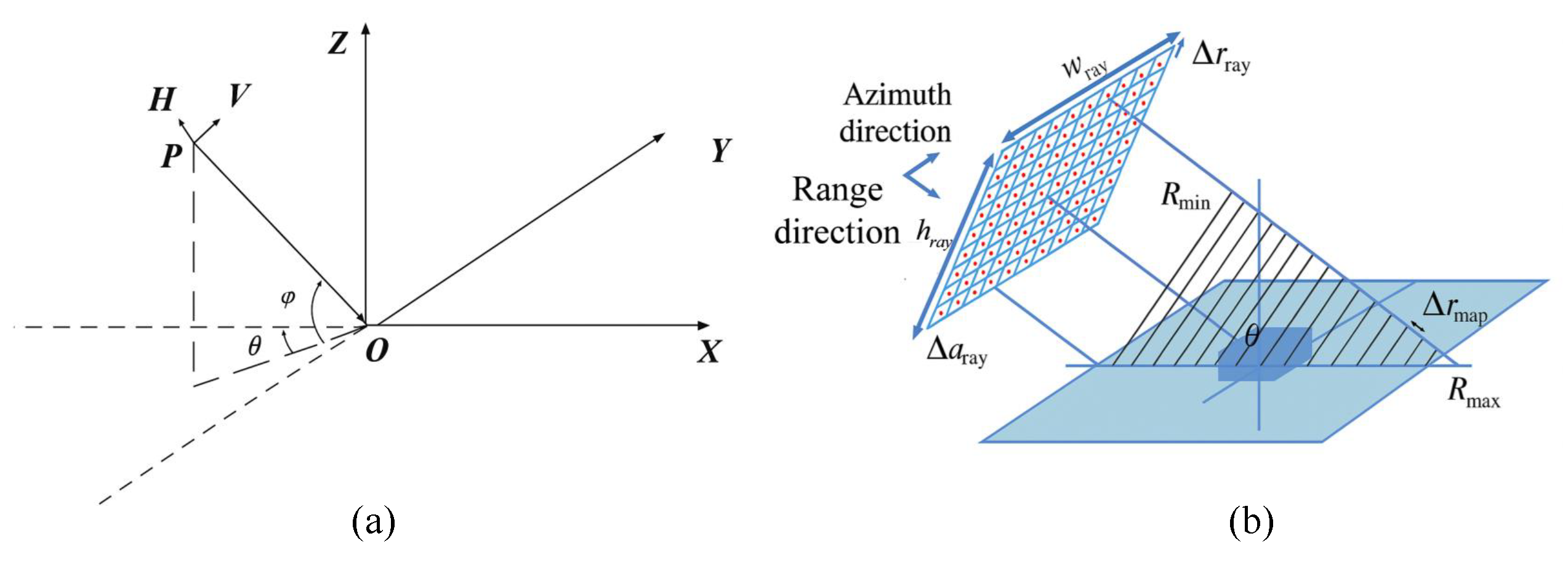
The specific workflow for electromagnetic scattering computation proceeds as follows. Using the geometric modeling results of the typical targets (i.e., target geometric model files in .pov format) along with the necessary radar system parameters for ray tracing simulation (X-band, HH polarisation, with an angular coverage from 10° to 360° at 10° intervals), the backscattering coefficient map is generated via the ray tracing method [40]. This map is subsequently converted into a header file for the electromagnetic scattering model to compute the target’s electromagnetic scattering parameters. Following the ray tracing process, the final electromagnetic modeling results of the scene targets are produced through image processing operations, including cropping and rotation. The coordinate system configuration and a schematic of the ray tracing process are illustrated in Figure 2.

Current spaceborne synthetic aperture radar (SAR) simulation methods typically integrate satellite platform models, ground scene models, and radar signal models to interactively simulate the reception process of actual echo signals. However, the high degree of coupling and complex interdependencies among these sub-models limit the modularity and scalability of the simulation system. Furthermore, the implementation of individual models often suffers from code redundancy and convoluted logic, resulting in poor maintainability and reusability. As observation scenarios continue to expand and resolution requirements become increasingly demanding, the computational complexity of echo data simulation grows exponentially, significantly extending the total simulation time. Thus, a major challenge in advancing SAR simulation technology is to effectively reduce computational complexity and time cost while preserving the imaging quality of the simulated outputs [41].

To address the aforementioned challenges, this paper proposes a novel multi-mode SAR echo simulation system characterised by high scalability and reusability. The system decomposes the echo simulation task into four core sub-algorithms that operate collaboratively, thereby reducing inter-model coupling at the architectural level and significantly enhancing system flexibility and parallelisation capabilities.

Satellite orbit dynamics modeling: Accurately generates satellite orbit and attitude information based on the spatial positioning constraints of the target region and input satellite parameters. The satellite motion equation is [42]:

$$\ddot{\mathbf{r}}\left(t\right)=-\mu {\displaystyle \frac{\mathbf{r}\left(t\right)}{r^3}}+{\mathbf{a}}_{\mathrm{pert}}\left(t\right)$$

(5)

where $\mathbf{r}\left(t\right)$ is the satellite position vector, $\mu$ is the Earth’s gravitational constant, and ${\mathbf{a}}_{\mathrm{pert}}\left(t\right)$ represents the perturbation acceleration (such as the gravitational pull of the sun and moon, atmospheric drag, etc.) The position of the satellite in the Earth-centered inertial system can be calculated from the six orbital elements $(a,e,i,\mathrm{\Omega },\omega ,M_0)$:

$$\mathbf{r}\left(t\right)=R_z\left(\mathrm{\Omega }\right)R_x\left(i\right)R_z\left(\omega \right){\mathbf{r}}_{\mathrm{orb}}\left(E\left(t\right)\right)$$

(6)

where ${\mathbf{r}}_{\mathrm{orb}}\left(E\right)={[a(\cos E-e),a\sqrt{1-e^2}\sin E,0]}^T$, the eccentric anomaly $E\left(t\right)$ is solved iteratively by the Kepler equation $E-e\sin E=M\left(t\right)$, and the mean anomaly $M\left(t\right)=n(t-t_0)$, $n=\sqrt{\mu /a^3}$.

Beam pointing trajectory deduction dynamically determines the instantaneous beam direction by integrating the platform’s three-axis attitude (pitch, yaw, and roll), antenna configuration, and orbital trajectory. This ensures that the computed beam orientation accurately reflects the platform’s full three-dimensional motion during imaging. The beam direction vector can be expressed as

$$\mathbf{b}\left(t\right)=R_z\left(\mathrm{\Omega }\right)R_x\left(i\right)R_z\left(\omega \right){\mathbf{b}}_0$$

(7)

where $R_x,R_z$ is the coordinate rotation matrix, $\mathrm{\Omega }$, i, and $\omega$ are the right ascension of the ascending node, the orbital inclination, and the argument of perigee in the orbital elements, respectively, and ${\mathbf{b}}_0$ is the initial antenna pointing vector.

Error modeling and injection: Enhances the realism and engineering applicability of the simulation by incorporating typical non-ideal factors—such as orbital errors, attitude disturbances, and system delays—into the simulation chain. The effect of velocity error on Doppler frequency modulation is

$$\Delta f_D\left(t\right)\approx {\displaystyle \frac{2}{\lambda }}\widehat{\mathbf{r}}\left(t\right)·\Delta \mathbf{v}\left(t\right)$$

(8)

where $\Delta f_D\left(t\right)$ is the Doppler frequency error, $\lambda$ is the wavelength, $\widehat{\mathbf{r}}\left(t\right)$ is the target pointing unit vector, and $\Delta \mathbf{v}\left(t\right)$ is the satellite velocity error vector. This formula shows that it is primarily affected by the flight direction velocity error and adjusts with changes in viewing angle. The impact of position error on Doppler cubic compensation:

$$R\left(t\right)\approx R_0+{\dot{R}}_{0}t+{\displaystyle \frac{1}{2}}{\ddot{R}}_0{t}^2+{\displaystyle \frac{1}{6}}{\stackrel{⃛}{R}}_0{t}^3$$

(9)

where $R\left(t\right)$ is the relative distance between the satellite and the target, ${\dot{R}}_0$, ${\ddot{R}}_0$, and ${\stackrel{⃛}{R}}_0$ are the first, second, and third derivatives of the equivalent slant range, respectively. Position measurement error $\Delta \mathbf{r}\left(t\right)$ affects the coefficients of each order, thereby affecting the accuracy of the cubic compensation.

Parallel computing optimisation for echo generation: Improves simulation efficiency through pulse coherence processing in the range-frequency domain combined with multi-threaded decomposition, enabling parallelised simulation of the echo reception process. The echo signal of a single point target can be simplified as follows [43]:

$$s_r(\tau ,\eta )=A_0{w}_r\left(\tau -{\displaystyle \frac{2R\left(\eta \right)}{c}}\right)w_a\left({\displaystyle \frac{\eta -{\eta }_c}{T_a}}\right)\exp \left(-j{\displaystyle \frac{4\pi R\left(\eta \right)}{\lambda }}\right)\exp \left(j\pi K_r{\left(\tau -{\displaystyle \frac{2R\left(\eta \right)}{c}}\right)}^2\right),$$

(10)

where $A_0$ is the complex amplitude including the target scattering and system gain, $w_r(·)$ and $w_a(·)$ are the range and azimuth envelope functions, $R\left(\eta \right)$ is the instantaneous slant range, c is the speed of light, $\lambda$ is the radar wavelength, ${\eta }_c$ is the reference azimuth time, $T_a$ is the azimuth window, and $K_r$ is the range chirp rate.

This approach effectively balances simulation performance with computational resource utilisation while maintaining accuracy, thereby offering theoretical support and engineering feasibility for the rapid simulation of large-scale, high-resolution SAR imaging tasks.

2.3. Implementation of a Multi-Target SAR Imaging Method

The core processing chain of spaceborne synthetic aperture radar (SAR) imaging typically involves steps such as range compression (RC), secondary range compression (SRC), azimuth matched filtering, and range cell migration correction (RCMC). Time-domain imaging methods are often associated with high computational complexity and low efficiency. As a result, mainstream SAR imaging algorithms are predominantly implemented in the frequency domain, including the range-Doppler (RD) algorithm, the chirp scaling (CS) algorithm, and the $\omega$-K algorithm algorithm [44,45]. These approaches perform key operations—including SRC, RCMC, and azimuth compression—within the Doppler domain.

This paper adopts the chirp scaling algorithm as the core method for the imaging process due to its advantages in high image quality, robustness against noise, and tolerance to incomplete data segments. These characteristics make it particularly suitable for application scenarios with constrained data acquisition conditions. The algorithm utilises chirp scaling to simultaneously accomplish range migration correction and range compression in the frequency domain, followed by azimuth compression to achieve fully focused two-dimensional imagery. The fundamental concept can be summarised as follows:

$$S_{\mathrm{RCMC}}(f_r,f_a)=S(f_r,f_a)·\exp \left(-j\pi {\displaystyle \frac{f_a^2}{K_r}}\right)$$

(11)

where $f_r$ is the range frequency, where $f_a$ is the azimuth frequency, and where $K_r$ is the chirp rate. Two-dimensional imaging focusing is then achieved through azimuth compression:

$$s_{\mathrm{image}}(x,y)={\mathcal{F}}^{-1}\left\{S_{\mathrm{RCMC}}(f_r,f_a)·H_a\left(f_a\right)\right\}$$

(12)

where $H_a\left(f_a\right)$ represents the azimuth matched filter and ${\mathcal{F}}^{-1}$ represents the two-dimensional inverse Fourier transform.

Finally, a multi-target dataset encompassing 15 typical targets across ground, maritime, and aerial categories was constructed. SAR images were generated at 10° intervals, yielding a total of 5940 images. A comparison between the 3D models and their corresponding SAR representations for all targets is provided in Figure 3. Each image was formatted to a size of 128 × 128 pixels, with amplitude values ranging from 0 to 255.

3. Proposed Method

This section details the proposed method’s key components: the overall network architecture, generator and discriminator models, angle encoder, attention mechanism, and loss function.

3.1. Proposed Network Framework

Synthetic Aperture Radar (SAR) images are characterised by significant noise and complex textures. As a result, StyleGAN2—known for its ability to capture intricate features and produce high-quality imagery—offers considerable potential for SAR image processing. This advantage stems primarily from its use of a mapping network that transforms random noise into a style space, allowing hierarchical control over various image layers (including both low-frequency and high-frequency information) to generate high-fidelity images with minimal distortion.

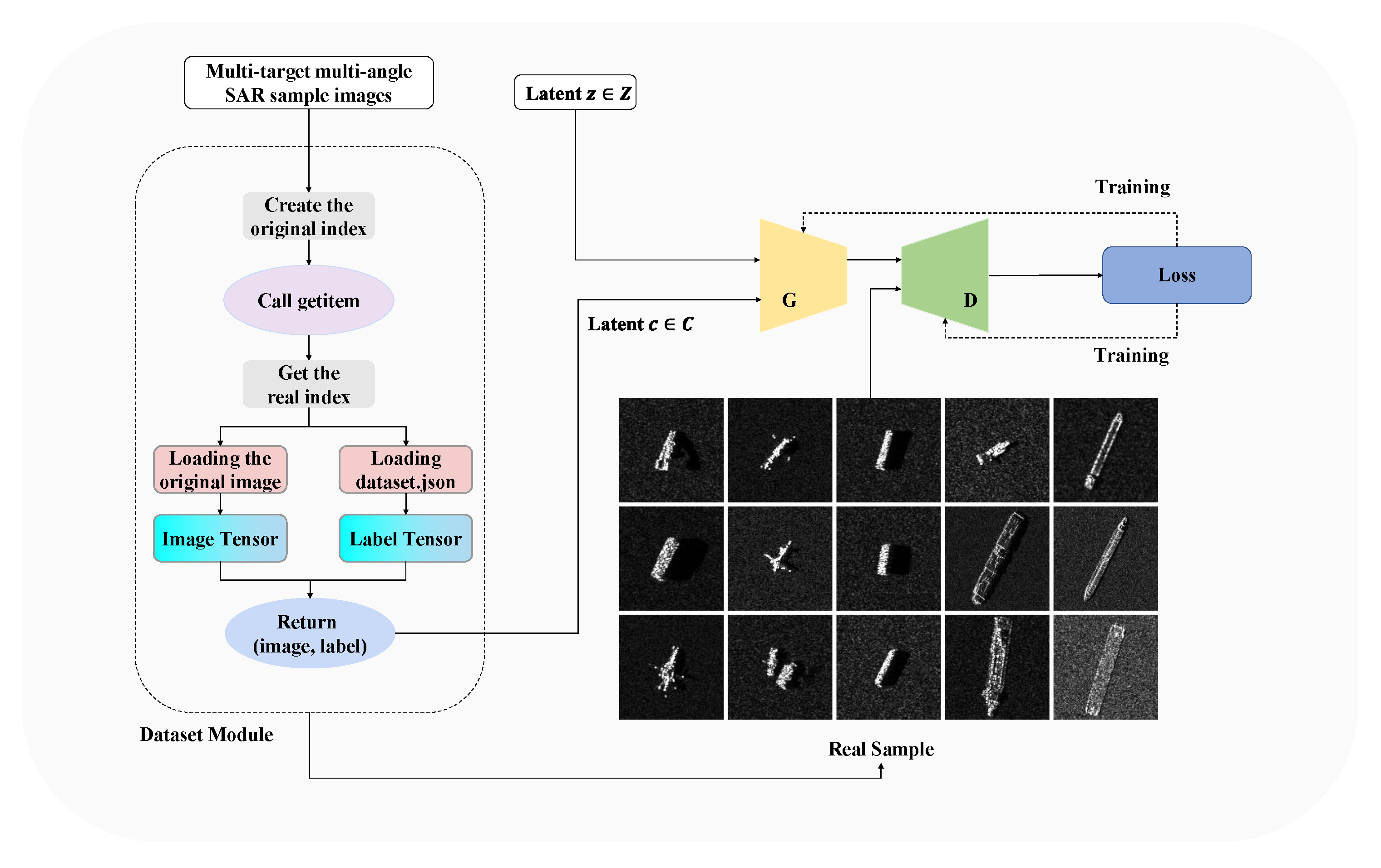
Furthermore, this work adopts a conditional StyleGAN2 framework, which incorporates additional conditional information alongside unconditional noise inputs. This enables the generator to produce images that adhere to specified conditions. In our method, the training dataset is first processed by the Dataset module, which returns images along with their corresponding conditional information. This conditional information—comprising the target category and angle label, both encoded in one-hot form—is then fed into the mapping network as conditional input to guide the image generation process. The inclusion of angle labels helps the generator better discern variations among different viewing angles, thereby alleviating the issue of limited angular samples in the dataset. Simultaneously, the introduction of target categories not only reduces the cost associated with multi-target training but also facilitates the comparison of feature and angle relationships across different targets, ultimately enhancing the generalisation capability of the network. The detailed network architecture is illustrated in Figure 4, and the formal expression of the conditional StyleGAN2 model is given as

$$G\left(z,c\right)=G\left(S\left(z\right)+E\left(c\right)\right)$$

(13)

where z is the latent noise vector, c denotes the conditional input consisting of target-category and angle labels, $S(·)$ is the mapping network that transforms z into an intermediate latent code, and $E(·)$ is the embedding network that projects the condition c into the same latent space. The combined representation $S\left(z\right)+E\left(c\right)$ serves as the condition-guided style vector for image synthesis.

3.2. Generator Module

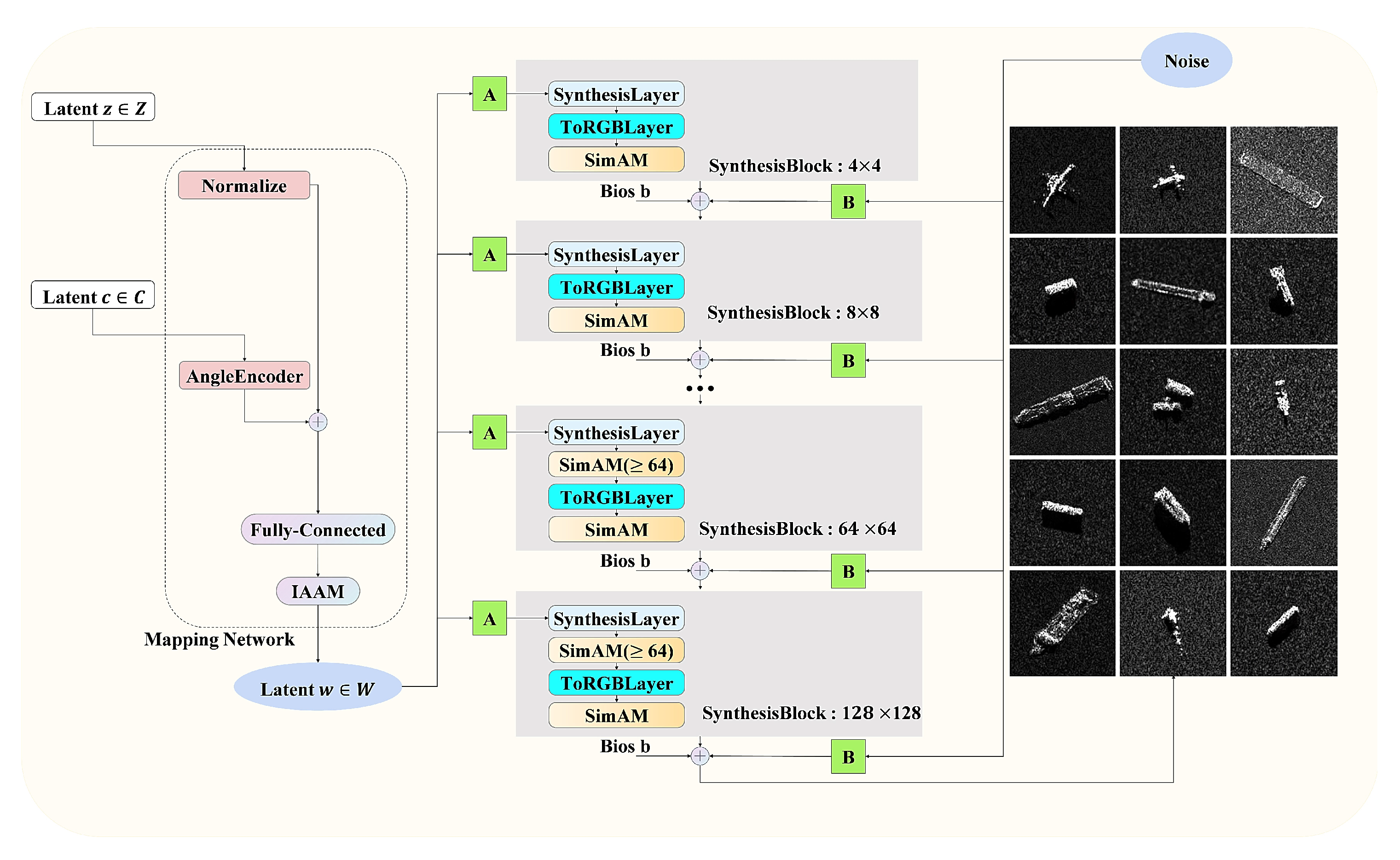
The generator consists of a mapping network and a synthesis network, as shown in Figure 5. Based on the StyleGAN2 architecture, the proposed generator incorporates an angle encoder (AngleEncoder) and a lightweight attention module (IAAM). The mapping network first modulates the style latent code, which is then progressively upsampled through a sequence of modulated convolutional layers to synthesise images from 4 × 4 up to 128 × 128 resolution. Each layer supports RGB output, yielding clearly structured and highly interpretable feature representations that make the model well-suited for multi-target and multi-angle SAR image generation. The main advantages of this generator design are summarised below:

1.

Target-category and angle labels (one-hot) are injected into the mapping network together with random noise to condition image synthesis. The angle encoder maps discrete angles to continuous, periodic-aware embeddings, enabling the generator to model inter-angle variations and alleviating limited-view/sample diversity.

2.

Conditioning on target categories reduces the cost of multi-target training and enables explicit comparison of feature–angle relationships across classes, thereby improving generalisation.

3.

We incorporate IAAM into the mapping network to strengthen conditional label representations, and add SimAM in the synthesis network to enhance fine-grained image details.

3.3. Discriminator Module

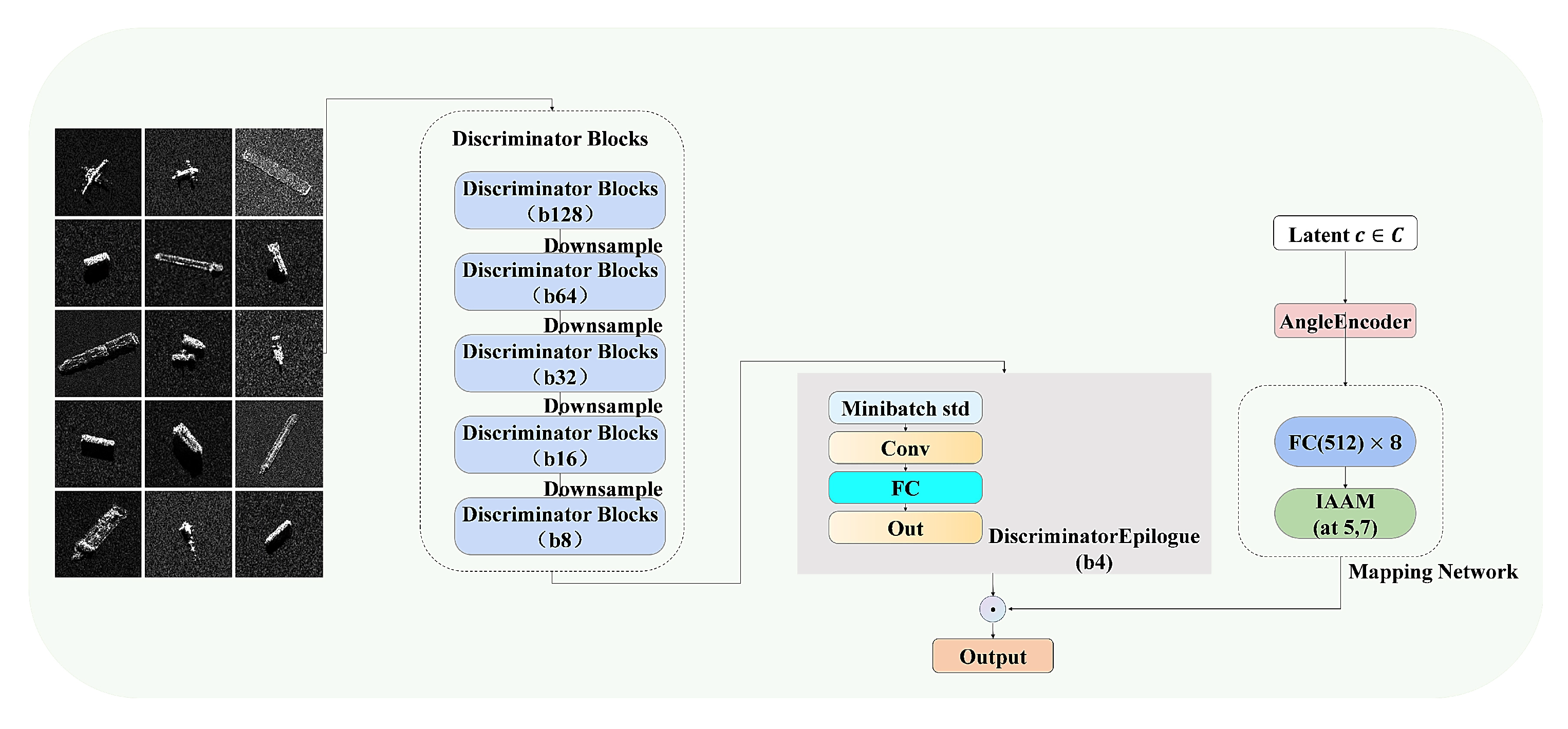
The detailed architecture of the proposed discriminator is illustrated in Figure 6.

The discriminator accepts either a generated SAR image or a real image sampled from the training dataset, together with the corresponding conditional information. Building upon the original StyleGAN2 discriminator, the proposed model incorporates a conditional discrimination mechanism. By integrating three modules—a conditional mapping network, a multi-scale feature pyramid, and a mini-batch statistical layer—it significantly enhances its capacity to assess angular consistency in generated images.

3.4. Angle Encoder

In the context of multi-target and multi-angle image generation, using one-hot encoding alone treats each angle as an entirely independent category. This approach fails to capture the inherent structure of the angular space, leading to issues such as excessive discreteness, lack of angular continuity, and difficulty in modeling periodicity [46,47]. To enhance the model’s ability to interpret angular information, this paper introduces a lightweight angle encoder module that incorporates sine and cosine periodic representations of angles. The angle encoder includes the following components:

• Discrete-angle selection: extract the 36 meaningful angle labels from the original 50-dimensional label set;
• Trigonometric precomputation: compute periodic features using sine and cosine functions;
• Feature transformation: concatenate, align dimensions, FC + LayerNorm + GELU;
• Output embedding: produce a 512-d embedding.

This design overcomes the limitations of one-hot encoding in representing continuity and periodicity—particularly the problem of boundary discontinuity—thereby strengthening the model’s perception of angular semantics and improving viewpoint control accuracy. The angle encoder is shown in the Figure 7, and the calculation process is as follows:

$$\mathbf{e}=\mathrm{GELU}\left(\mathrm{LayerNorm}\left(\mathrm{Linear}\left([\mathbf{o};{\mathbf{o}}^{\top }\sin \left(\theta \right);{\mathbf{o}}^{\top }\cos \left(\theta \right);{\mathbf{0}}_{34}]\right)\right)\right)$$

(14)

where: $\mathbf{o}\in {\{0,1\}}^K$ is the input one-hot angle vector, $K=36$ is the number of discrete angles, $\theta ={[1·{10}^{\circ },\dots ,K·{10}^{\circ }]}^{\top }$ (converted to radians), ${\mathbf{0}}_{34}$ is a zero-padding vector, ‘Linear’ denotes the trainable linear layer with parameters $W,b$, and $\mathbf{e}\in {\mathbb{R}}^E$ is the output angle embedding ($E=512$).

3.5. Attention Module

3.5.1. SimAM Attention Module

To further improve the detail quality of SAR images, the SimAM module [48] was integrated into the generator network. As a lightweight and parameter-free attention mechanism, SimAM enhances feature representation in image generation tasks. It introduces no additional learnable parameters and provides an inductive bias that enhances salient feature representation without increasing model capacity, thereby mitigating overfitting in limited-sample scenarios. Its minimal parameter footprint makes it particularly suitable for multi-view SAR image generation, which is often challenged by significant target deformation, highly nonlinear feature variations, strong reliance on fine details (e.g., edges and scattering centers), and substantial background interference, including shadows and artifacts. A block diagram illustrating the structure of the SimAM attention module is provided in Figure 8a. The computational process of the SimAM attention module is as follows:

Let $\mathbf{X}\in {\mathbb{R}}^{C\times H\times W}$ denote the input feature map, where C is the number of channels and $H,W$ are spatial dimensions. We index a channel by $c\in \{1,\dots ,C\}$ and a flattened spatial location by $t\in \{1,\dots ,HW\}$; let $x_{c,t}\in \mathbb{R}$ be the activation at channel c and position t. Denote by ${\mu }_{c,t}$ and ${\sigma }_{c,t}^2$ the mean and variance of activations in channel c computed excluding position t. Let $\lambda >0$ be a small regularizer (we use $\lambda ={10}^{-4}$). The scalar energy $e_{c,t}^{*}$ and the energy tensor $\mathbf{E}\in {\mathbb{R}}^{C\times H\times W}$ (with ${\left[\mathbf{E}\right]}_{c,t}=e_{c,t}^{*}$) are given by

$$e_{c,t}^{*}={\displaystyle \frac{4{(x_{c,t}-{\mu }_{c,t})}^2+4{\sigma }_{c,t}^2+2\lambda }{{(x_{c,t}-{\mu }_{c,t})}^2+2{\sigma }_{c,t}^2+2\lambda }}.$$

(15)

Following the “lower energy = more important” principle, we form an attention map via element-wise inversion and sigmoid, and obtain the enhanced feature map

$$\tilde{\mathbf{X}}=\mathbf{X}\otimes \sigma \left({\mathbf{E}}^{-1}\right),$$

(16)

where $\sigma (·)$ is the element-wise sigmoid, ⊗ denotes element-wise multiplication, and ${\left[{\mathbf{E}}^{-1}\right]}_{c,t}={\displaystyle \frac{1}{e_{c,t}^{*}+\epsilon }}$ with a small $\epsilon >0$ to avoid division by zero. Equivalently, at the scalar level ${\tilde{x}}_{c,t}=x_{c,t}\sigma \left(1/(e_{c,t}^{*}+\epsilon )\right)$.

3.5.2. IAAM Attention Module

Although SimAM exhibits notable effectiveness in modeling image features, it is fundamentally designed for spatially-structured feature maps in the format of a 4D tensor [B, C, H, W] (B: batch, C: channel, H: height, W: width). In this architecture, attention weights are derived independently for each spatial location through an energy function, rendering the mechanism particularly suitable for neuron-level feature enhancement within convolutional networks. However, mapping networks—such as those used for latent space transformation in generative adversarial networks (GANs) or multi-layer perceptrons—commonly process high-dimensional vectorized inputs (e.g., of shape [B, C]) that lack spatial extent. In such contexts, the direct application of SimAM not only introduces computational redundancy but also underutilizes its inherent capability for spatial feature modeling.

To more effectively strengthen the representation of conditional labels in mapping networks, we propose IAAM (Instance-wise Adaptive Attention Module), a lightweight, vector-oriented variant of SimAM, specifically designed for instance-level vector representation. Similar to SimAM, IAAM employs an energy function to compute attention values; however, it operates solely across the channel dimension. IAAM computes the channel-wise energy and attention as:

$${\tilde{\mathbf{x}}}_i={\mathbf{x}}_i·\sigma \left(-\left({\displaystyle \frac{{({\mathbf{x}}_i-\mu )}^2}{4({\sigma }^2+\epsilon )}}+0.5\right)\right),\mu ={\displaystyle \frac{1}{C}}\sum _{j=1}^C{\mathbf{x}}_j,{\sigma }^2={\displaystyle \frac{1}{C}}\sum _{j=1}^C{({\mathbf{x}}_j-\mu )}^2$$

(17)

where $\mathbf{x}=({\mathbf{x}}_1,\dots ,{\mathbf{x}}_C)\in {\mathbb{R}}^C$ is the input vector of a single instance, $\mu$ and ${\sigma }^2$ are the channel-wise mean and variance, $\epsilon >0$ is a small constant for numerical stability, $\sigma (·)$ is the sigmoid function, and ${\tilde{\mathbf{x}}}_i$ is the attended output.

IAAM is parameter-free in our implementation and reduces the complexity per sample from $\mathcal{O}\left(CHW\right)$ (SimAM on feature maps) to $\mathcal{O}\left(C\right)$ (IAAM on vectors). Numerical complexity examples are given in

Table 2. Numerical complexity examples (per-sample FLOPs) for typical configs.

Module	Input Shape	Trainable Params	FLOPs per Sample
SimAM	[B, 512, 16, 16]	0	1,311,744
IAAM	[B, 512]	0	5122

. SimAM attains approximately 1,311,744 FLOPs per sample, whereas IAAM (vector) requires approximately 5122 FLOPs per sample. The difference is about $1.31\times {10}^6$ FLOPs, indicating that SimAM is roughly 256 times more computationally expensive than IAAM.

Without requiring any trainable parameters or elaborate components, IAAM maintains high computational efficiency and is well-adapted to vector-level representation learning tasks, including those common in mapping networks. The block diagram of the IAAM attention module is shown in Figure 8b.

Table 3. Comparison of different attention mechanisms.

Feature	SE [49]	CBAM [50]	IAAM
Attention Dimension	1D	2D	1D
Trainable parameters	✔	✔	×
Computational complexity	$\mathcal{O}\left(C^2\right)$	$\mathcal{O}\left(HWC\right)$	$\mathcal{O}\left(BC\right)$
Instance Adaptation	×	×	✔
Energy function guidance	×	×	✔
Gradient stability	Medium	Medium	High

Legend: ✔ = present / Yes; × = absent / No.

compares the module features of IAAM and various attention modules.

3.6. Loss Function

3.6.1. Generator Adversarial Loss

The generator adversarial loss follows the StyleGAN2 formulation, where the conventional $-\log \left(\mathrm{sigmoid}\right(D\left(G\right(z\left)\right)\left)\right)$ term is replaced by the numerically stable softplus function:

$${\mathcal{L}}_G={\mathbb{E}}_{\mathbf{z}\sim p\left(\mathbf{z}\right),\mathbf{c}\sim p\left(\mathbf{c}\right)}\left[\mathrm{softplus}\left(-D\left(G\right(\mathbf{z},\mathbf{c}\left)\right)\right)\right].$$

(18)

Here, $\mathbf{z}$ denotes the latent noise vector, $\mathbf{c}$ the conditional information (category or angle label), $G(·)$ and $D(·)$ represent the generator and discriminator, respectively, and $\mathrm{softplus}(·)$ provides smoother gradients and enhanced numerical stability.

3.6.2. Discriminator Adversarial Loss

The discriminator aims to assign higher scores to real samples and lower scores to generated ones, formulated as

$${\mathcal{L}}_D={\mathbb{E}}_{(\mathbf{x},\mathbf{c})\sim p_{\mathrm{data}}}\left[\log \left(1+\exp (-D(\mathbf{x},\mathbf{c}\left)\right)\right)\right]+{\mathbb{E}}_{\mathbf{z},\mathbf{c}}\left[\log \left(1+\exp \left(D\right(G(\mathbf{z},\mathbf{c}),\mathbf{c}\left)\right)\right)\right],$$

(19)

where $\mathbf{x}$ denotes a real image sampled from the data distribution $p_{\mathrm{data}}$; $\mathbf{z}$ is the latent vector drawn from the prior distribution $p\left(\mathbf{z}\right)$ (usually standard normal); $\mathbf{c}$ represents the conditional information (e.g., category or angle label); $G(·)$ and $D(·)$ denote the generator and discriminator networks, respectively; and $\log (1+\exp (·\left)\right)$ is the numerically stable softplus function used for adversarial optimization.

3.6.3. Perceptual Loss

To improve visual quality and semantic consistency, a VGG16-based perceptual loss is adopted:

$${\mathcal{L}}_{\mathrm{perc}}={\mathbb{E}}_{\mathbf{z},\mathbf{c},\mathbf{x}}\left[{\parallel {\varphi }^{[1:16]}\left(\mathbf{x}\right)-{\varphi }^{[1:16]}\left(G(\mathbf{z},\mathbf{c})\right)\parallel }_1\right],$$

(20)

where $\varphi (·)$: VGG16 network pre-trained on ImageNet, ${\varphi }^{[1:16]}(·)$: means taking the first 16 layers of VGG-16 as feature extractors, ${\parallel ·\parallel }_1$: L1 norm (i.e., sum of absolute errors). This encourages the generated images to resemble real ones in the feature space. This constraint encourages the generated images to resemble real images in the VGG feature space. Although VGG16 is pretrained on natural images, its shallow and mid-level features primarily capture generic visual patterns such as edges and textures, which exhibit reasonable generalization to SAR imagery [51,52].

3.6.4. R1 Regularization

Following StyleGAN2, an ${\mathcal{R}}_1$ gradient penalty regularizes the discriminator [53] to prevent overfitting:

$${\mathcal{L}}_{R_1}={\displaystyle \frac{{\gamma }_1}{2}}{\mathbb{E}}_{(\mathbf{x},\mathbf{c})\sim p_{\mathrm{data}}}\left[{∥{\nabla }_{\mathbf{x}}D(\mathbf{x},\mathbf{c})∥}_2^2\right],$$

(21)

where $\mathbf{x}$ is a real image sampled from the data distribution $p_{\mathrm{data}}$, $\mathbf{c}$ denotes the conditioning vector (if any), $D(·,·)$ is the discriminator, ${\nabla }_{\mathbf{x}}D$ the gradient of D w.r.t. $\mathbf{x}$, and ${\gamma }_1>0$ is the R₁ regularization strength (we use ${\gamma }_1=10$ by default). This penalty term is computed exclusively on real images and controls the discriminator’s gradients to mitigate overfitting.

4. Experiments and Results

4.1. Experimental Datasets

This study employs two distinct datasets: (1) a self-constructed multi-target, multi-angle synthetic aperture radar (SAR) dataset, and (2) the SAMPLE dataset [54], which is derived from MSTAR benchmark measurements. Both datasets are split into training and testing subsets in an 8:2 ratio. The self-constructed SAR dataset was acquired in the X-band under HH polarisation, with an image resolution of 128 × 128. It comprises 15 types of typical civilian targets. The imaging geometry is fixed at a pitch angle of 60°, while the azimuth angle ranges from 10° to 360° in increments of 10°. A comparison between optical images and their corresponding SAR images for the targets in this dataset is provided in Figure 9. The SAMPLE dataset consists of 10 types of military vehicles, including 2S1, BMP2, BTR70, M1, M2, M35, M60, M548, T72, and ZSU23. Each image has a resolution of 128 × 128. The data were collected at a pitch angle of 17°, with azimuth angles varying from 10° to 80° in steps of 1°. The labels in this dataset are one-hot encoded to represent both target categories and angle categories, resulting in 10 class labels for targets and 70 class labels for angles. A comparison between optical and corresponding SAR images for the SAMPLE dataset targets is presented in Figure 10.

4.2. Experimental Settings

The experiments were run on a Linux workstation with an NVIDIA V100 GPU (NVIDIA Corporation, Santa Clara, CA, USA; 16 GB) and an Intel Core processor (Intel Corporation, Santa Clara, CA, USA; 6 cores, 49 GB RAM). The implementation was based on PyTorch 2.4.1 and executed on a system with CUDA Toolkit 12.1 (NVIDIA Corporation). All images were rescaled to a resolution of 128 × 128 pixels. The model was trained using the Adam optimiser with a learning rate of 0.0025 and a batch size of 8. The generator employed a latent space dimension of 512.

4.3. Evaluation Metrics

To comprehensively evaluate the quality of the generated SAR images from multiple perspectives, this paper adopts a multi-metric evaluation approach. Specifically, the evaluation is divided into two categories: Distributional and perceptual metrics, and Diversity and memorization checks. The former includes the Fréchet Inception Distance (FID), Kernel Inception Distance (KID), and Multi-Scale Structural Similarity Index (MS-SSIM), which are used to quantify the quality and diversity of the generated images. The latter is employed to assess the alignment between the generated distribution and the real distribution, as well as to examine whether the model is overfitting.

4.3.1. Distributional and Perceptual Metrics [55]

The Fréchet Inception Distance (FID) quantifies the discrepancy between the distributions of real and generated images by comparing Gaussian approximations (mean and covariance) of their deep features; it is particularly sensitive to global statistical deviations and a lower FID indicates closer alignment to the real data distribution:

$$\mathrm{FID}={\parallel {\mu }_r-{\mu }_g\parallel }_2^2+\mathrm{Tr}\left({\mathrm{\Sigma }}_r+{\mathrm{\Sigma }}_g-2{\left({\mathrm{\Sigma }}_r{\mathrm{\Sigma }}_g\right)}^{1/2}\right),$$

(22)

where ${\mu }_r,{\mathrm{\Sigma }}_r$ represent the mean and covariance of the real image features, and ${\mu }_g,{\mathrm{\Sigma }}_g$ represent those of the generated image features. A lower FID value indicates that the distribution of generated images is closer to that of the real images.

As an unbiased alternative, the Kernel Inception Distance (KID) measures the squared Maximum Mean Discrepancy (MMD) between real and generated feature sets using a polynomial kernel; lower KID values indicate better distributional match:

$$\mathrm{KID}={\displaystyle \frac{1}{m(m-1)}}\sum _{i\ne j}k(x_i,x_j)+{\displaystyle \frac{1}{n(n-1)}}\sum _{i\ne j}k(y_i,y_j)-{\displaystyle \frac{2}{mn}}\sum _{i,j}k(x_i,y_j),$$

(23)

where $x_i\sim P_r$ denotes a real sample, $y_j\sim P_g$ denotes a generated sample, and $k(·,·)$ is a polynomial kernel function. A lower KID value indicates a smaller discrepancy between the two distributions.

The Multi-Scale Structural Similarity (MS-SSIM) [56] index evaluates structural fidelity across scales by combining luminance, contrast and structure comparisons; values lie in $[0,1]$ with values closer to 1 indicating higher perceptual/structural similarity:

$$\mathrm{MS}\text{-}\mathrm{SSIM}(x,y)={\left[l_M(x,y)\right]}^{{\alpha }_M}\prod _{j=1}^M{\left[c_j(x,y)\right]}^{{\beta }_j}{\left[s_j(x,y)\right]}^{{\gamma }_j},$$

(24)

where M is the number of scales, and ${\alpha }_M,{\beta }_j,{\gamma }_j$ are weighting factors. An MS-SSIM value closer to 1 indicates higher multi-scale structural similarity between the generated image and the real image.

4.3.2. Diversity and Memorization Checks

The PRD curve quantifies the trade-off between precision (sample quality) and recall (sample diversity) across different density ratios $\beta$. Given feature histograms $\mathbf{p}$ and $\mathbf{q}$ estimated from real and generated samples via K-means clustering, the precision–recall pair is computed as

$$\mathrm{Precision}\left(\beta \right)=\sum _i\min (q_i,\beta p_i),\mathrm{Recall}\left(\beta \right)=\sum _i\min (p_i,q_i/\beta ),$$

(25)

and the best F1-score [57] is defined as

$${\mathrm{PRD}}_{\mathrm{best}\_\mathrm{F}1}=\underset{\beta }{\max }{\displaystyle \frac{2\mathrm{Precision}\left(\beta \right)\mathrm{Recall}\left(\beta \right)}{\mathrm{Precision}\left(\beta \right)+\mathrm{Recall}\left(\beta \right)}}.$$

(26)

A higher ${\mathrm{PRD}}_{\mathrm{best}\_\mathrm{F}1}$ indicates both high-quality and diverse generation.

We measure memorization using a nearest-neighbor-based proxy following the implementation of the Alan Turing Institute [58]. The theoretical leave-one-out (LOO) log-probability definition is given by

$$P_A(x\mid D)=\int p(x\mid D,a)p\left(a\right)\mathrm{d}a\approx {\displaystyle \frac{1}{T}}\sum _{t=1}^{T}p(x\mid D,a_t),$$

(27)

$$M_{\mathrm{LOO}}=\log P_A(x_i\mid D)-\log P_A(x_i\mid D_{\left[n\right]\setminus i}),$$

(28)

where $P_A(x\mid D)$ denotes the expected likelihood under randomized algorithm instances a, and $M_{\mathrm{LOO}}$ quantifies how much more likely $x_i$ is when included in the training set compared to when it is excluded.

Let $\varphi (·)$ be a deep feature extractor, and denote by ${\parallel ·\parallel }_2$ the Euclidean distance in the feature space. The implemented nearest-neighbor-based approximation to memorization is computed as

$$d_{\mathrm{gen}\text{-}\mathrm{to}\text{-}\mathrm{train}}={\displaystyle \frac{1}{N_g}}\sum _{i=1}^{N_g}\underset{1\le j\le N_r}{\min }{\parallel {\mathbf{f}}_g^{\left(i\right)}-{\mathbf{f}}_r^{\left(j\right)}\parallel }_2,$$

(29)

where ${\mathbf{f}}_g^{\left(i\right)}$ and ${\mathbf{f}}_r^{\left(j\right)}$ denote the feature representations of generated and real images, respectively.

$$d_{\mathrm{gen}\to \mathrm{train}}\left(x_i^{\left(g\right)}\right)=\underset{1\le j\le N_r}{\min }{\parallel \varphi \left(x_i^{\left(g\right)}\right)-\varphi \left(x_j^{\left(r\right)}\right)\parallel }_2,$$

(30)

$${\tau }_p=\mathrm{Percentile}\left(\left\{d_{\mathrm{train}\_\mathrm{self}}\left(x_j^{\left(r\right)}\right)\right\},p\%\right),$$

(31)

where ${\tau }_p$ is the p-th percentile of nearest-neighbor distances among real training samples (typically $p=5\%$).

Finally, the memorization score is defined as

$${\mathrm{MemorizationScore}}_p={\displaystyle \frac{1}{N_g}}\sum _{i=1}^{N_g}\mathbf{1}\left(d_{\mathrm{gen}\to \mathrm{train}}\left(x_i^{\left(g\right)}\right)\le {\tau }_p\right),$$

(32)

which measures the fraction of generated samples that are closer to the training set than the threshold ${\tau }_p$.

4.4. Qualitative Evaluation

In this experiment, the evaluation is performed at the image level and feature level by evaluating the generated images and deep feature visualisation, respectively.

4.4.1. Multi-Target Multi-Angle Image Generation

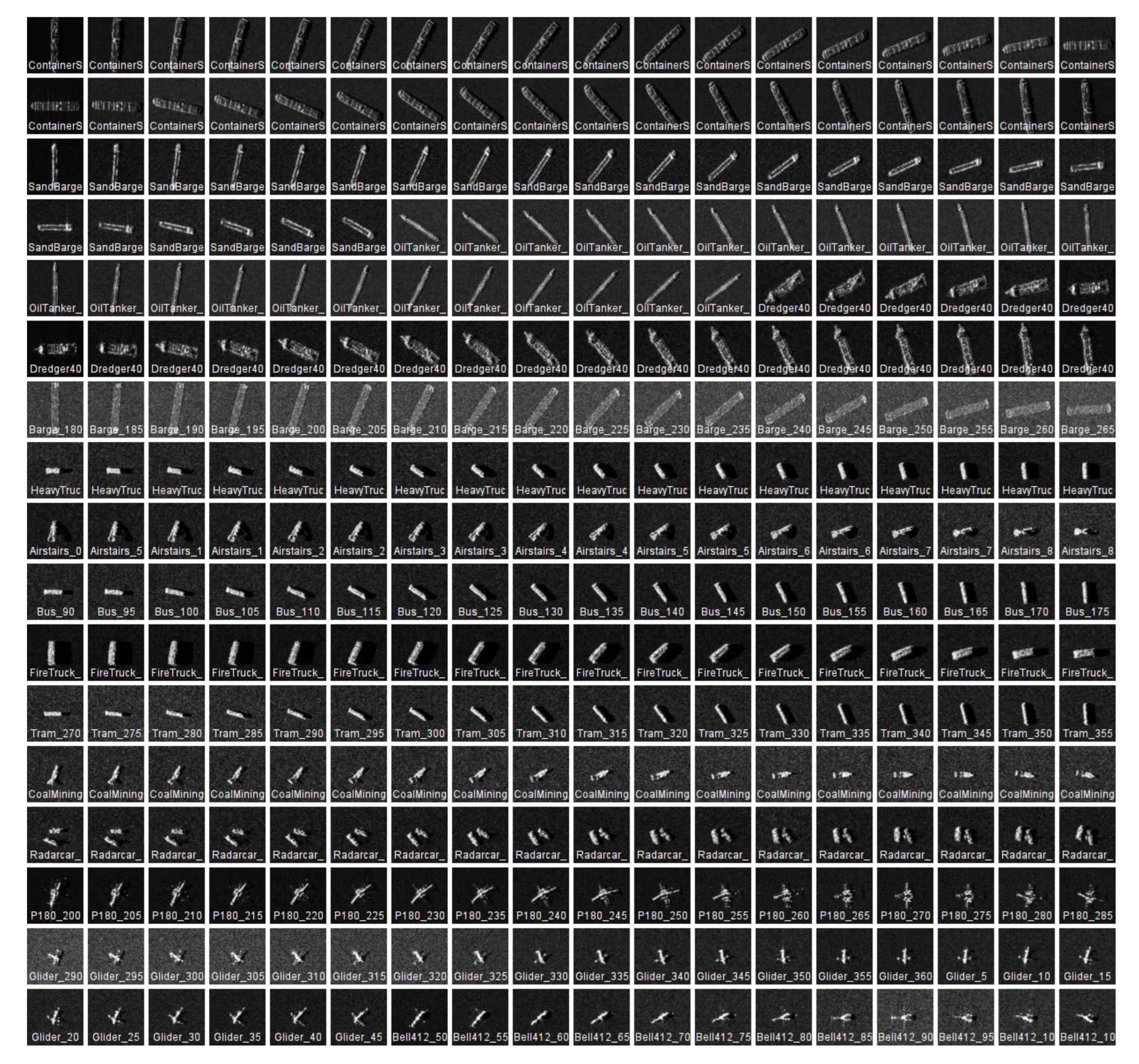
For the self-constructed dataset, Figure 11 illustrates the use of StyleGAN2 to augment a multi-target, multi-angle SAR image collection. During training, 15 target category labels and 36 angle labels were used to guide the network in capturing both the variations and consistencies in target appearance across different azimuth angles. By integrating these labels with an angle interpolation strategy, synthetic SAR images were generated covering the full azimuth range from 0° to 360° at intervals of 5°. This method provides an effective means of filling in missing angular perspectives in SAR target datasets. Note that all generated samples are shown at 5° intervals to demonstrate continuous angular transitions. The figure is intended for completeness rather than comparative counting.

To facilitate clear visualisation, the figure composites generated examples across all fifteen target categories, each depicted over a designated angular segment: Container Ship (0–175°), Sand Barge (180–295°), Oil Tanker (300–55°), Dredger4017 (60–175°), Barge (180–265°), Heavy Truck (270–355°), Airstairs (0–85°), Bus (90–175°), Fire Truck (180–265°), Tram (270–355°), Coal Mining Truck (20–105°), Radarcar (110–195°), P180 (200–285°), Glider (290–45°), and Bell412 (50–105°). The results demonstrate that the model generates images with enhanced clarity, standardised shapes and structures, and consistently high quality across all angles, with no noticeable blurring or overlapping artefacts.

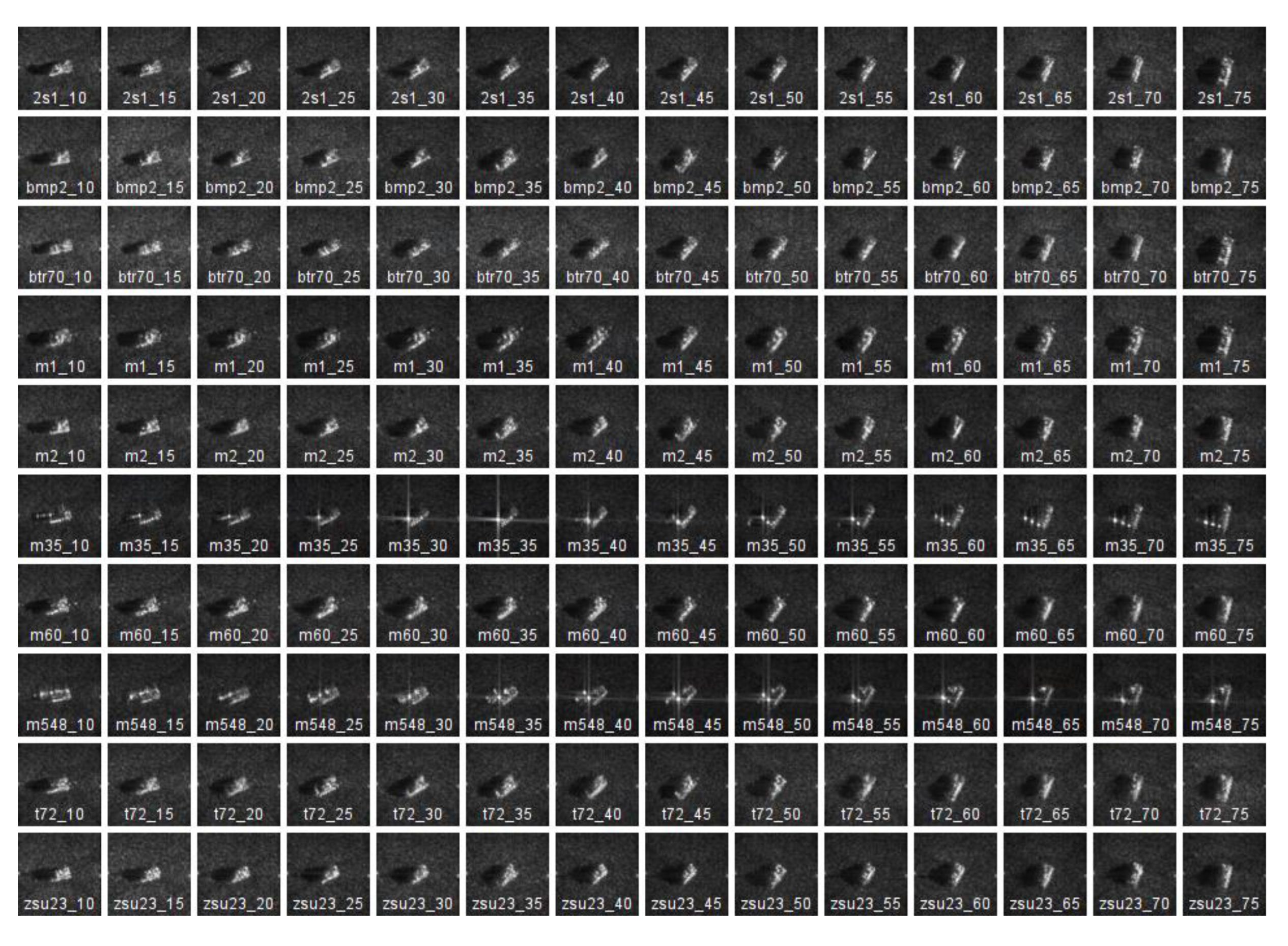
Figure 12 illustrates a sample augmentation result based on the SAMPLE dataset, using 10 target category labels and 70 angle labels to guide the image generation process. The generated images span azimuth angles from 10° to 75° at regular 5° intervals. The results show that all targets remain clearly visible and well-defined across every angle, with no discernible blurring or ghosting artifacts, reflecting consistently high image quality throughout.

4.4.2. Ablation Experiments

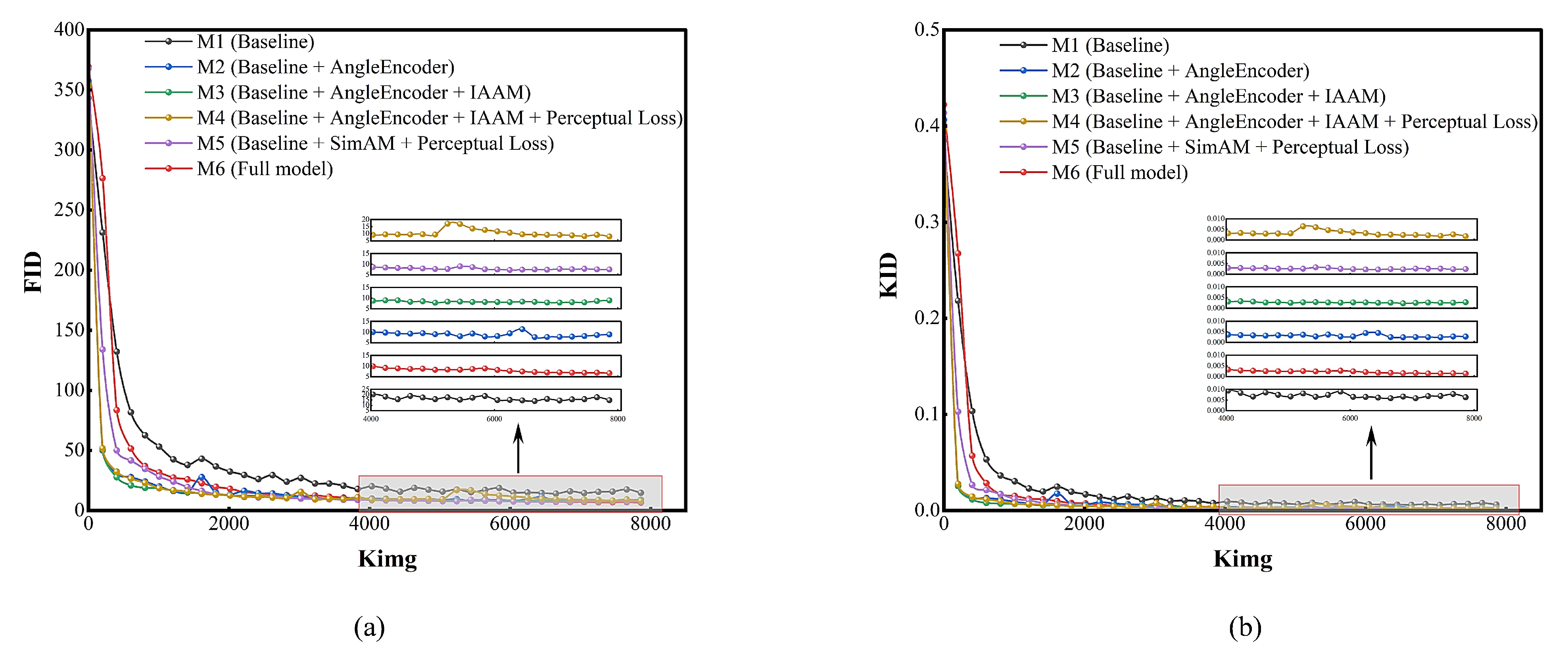
To evaluate the contribution of each component in the proposed model, we performed a series of ablation studies on a self-constructed multi-target, multi-angle SAR dataset. Under consistent training and data settings, six model configurations (denoted M1–M6) were compared: M1 (Baseline): original StyleGAN2; M2 (Baseline + AngleEncoder): StyleGAN2 with the angle encoder; M3 (Baseline + AngleEncoder + IAAM): add the proposed IAAM module; M4 (Baseline + AngleEncoder + IAAM + Perceptual Loss): M3 plus the perceptual loss; M5 (Baseline + SimAM + Perceptual Loss): baseline augmented by SimAM and perceptual loss (no IAAM/AngleEncoder); M6 (Full model): Baseline + AngleEncoder + IAAM + SimAM + Perceptual Loss. The Fréchet Inception Distance (FID) and Kernel Inception Distance (KID) were adopted as the primary quantitative metrics.

The corresponding training FID/KID curves for these six models are presented in Figure 13 (see legend for mapping M1–M6 to colors). The horizontal axis represents the number of training steps (in thousands of images, Kimg), with a detailed view from 4000 to 8000 Kimg provided in the inset at the lower right.

Table 4. Ablation results: FID and KID (mean ± std) for six model configurations (M1–M6).

Model	FID (Mean ± Std)	KID (Mean ± Std)
M1 (Baseline)	$14.758\pm 0.134$	$0.00628\pm 0.00018$
M2 (Baseline + AngleEncoder)	$8.977\pm 0.100$	$0.00293\pm 0.00013$
M3 (Baseline + AngleEncoder + IAAM)	$8.874\pm 0.018$	$0.00272\pm 0.00003$
M4 (Baseline + AngleEncoder + IAAM + Perceptual Loss)	$8.002\pm 0.033$	$0.00174\pm 0.00008$
M5 (Baseline + SimAM + Perceptual Loss)	$7.466\pm 0.016$	$0.00238\pm 0.00004$
M6 (Full model)	$6.541\pm 0.123$	$0.00139\pm 0.00012$

reports the quantitative results (mean ± std) for the six evaluated model configurations in terms of FID and KID. Relative to the baseline (M1), the inclusion of the angle encoder alone (M2) reduces the mean FID by approximately 39.2% (from 14.758 to 8.977) and KID by about 53.3%, indicating that the angle encoder substantially improves generation fidelity and mitigates mode oscillations. Adding the proposed IAAM module (M3) yields a modest additional improvement (FID down to 8.874, KID to 0.00272). Further incorporating the perceptual loss (M4) achieves more pronounced gains, reducing FID to 8.002 (≈45.8%reduction vs. M1) and KID to 0.00174 (≈72.3%reduction vs. M1). Replacing IAAM with SimAM (M5) also provides notable benefits (FID 7.466, KID 0.00238), suggesting that the perceptual constraint synergizes well with attention mechanisms. Finally, the full model (M6: AngleEncoder + IAAM + SimAM + Perceptual Loss) achieves the best overall performance (FID $6.541\pm 0.123$, KID $0.00139\pm 0.00012$), corresponding to approximately 55.7% and 77.9% reductions in FID and KID, respectively, relative to the baseline. The introduction of the angle encoder alone leads to a notable decrease in FID and alleviates early training oscillations. Subsequent incorporation of IAAM and perceptual loss further reduces the FID mean and results in a smoother curve. The combination of SimAM and perceptual loss also contributes significantly to the preservation of structural and detailed features. In conclusion, the ablation study confirms that the angle encoder plays a critical role in performance improvement, while the attention mechanism and perceptual loss collectively enhance both generation quality and training stability. The complete model achieves the lowest FID among all configurations.

4.4.3. Feature Visualization

In feature visualisation, we employed t-SNE [59] for target type discrimination and UMAP [60] for azimuth distribution analysis. Specifically, t-SNE inherently emphasises discrete clustering and local noise separation, thereby enhancing the inter-class distinguishability among different target categories. In contrast, UMAP is more suitable for continuous variables, such as azimuth, as it preserves the global geometric structure and effectively reveals the cyclic nature of angular variation (ranging from 10° to 360°). This complementary selection allows us to simultaneously demonstrate both categorical separability and angular continuity within a unified framework.

Furthermore, to compare the distributions of different angular features, we designed two visualisation modes: single-point mode and circular-cluster mode. The single-point mode represents each observed azimuth as an individual feature point, which intuitively reflects the overall distribution trend of different angles in the feature space. However, this mode lacks information on intra-class variation and fails to capture the angular uncertainty inherent in practical SAR imaging, which arises from sensor precision limitations or target posture perturbations. In contrast, the circular-cluster mode introduces slight Gaussian perturbations to the azimuth values, forming compact point clusters for each angle. This approach not only more closely aligns with real imaging conditions but also effectively reveals the continuity and periodicity of angular distribution (exhibiting a circular characteristic from 10° to 360°), while highlighting the model’s robustness to angular disturbances.

As illustrated in Figure 14a and Figure 15a, the self-constructed multi-target SAR dataset (15 targets) and the MTAR dataset (10 targets) exhibit well-separated feature distributions. The inter-class boundaries are clearly defined with minimal overlap, highlighting the effectiveness of the target-conditional one-hot encoding strategy. Figure 14b,c and Figure 15b,c further depict the distributions of angle variations.

Specifically, the UMAP dimensionality reduction results are shown for targets sampled in the embedding space with angular step sizes of 10°, covering the ranges of 10–360° and 10–70°, respectively. The resulting embeddings form a continuous, approximately circular trajectory in the two-dimensional space, with angle samples arranged in a clockwise order. Neighboring angular samples remain closely connected, producing a smooth transition across the full observation range. This behavior demonstrates that the extracted features faithfully capture the underlying variations in target observation angles. Moreover, the sequentially annotated angle labels in the figures clearly illustrate the correspondence between the learned feature embeddings and the true angular positions. Overall, the distribution results confirm the capability of the proposed method to preserve angular continuity and verify the effectiveness and feasibility of the designed angle encoder.

4.5. Quantitative Evaluation

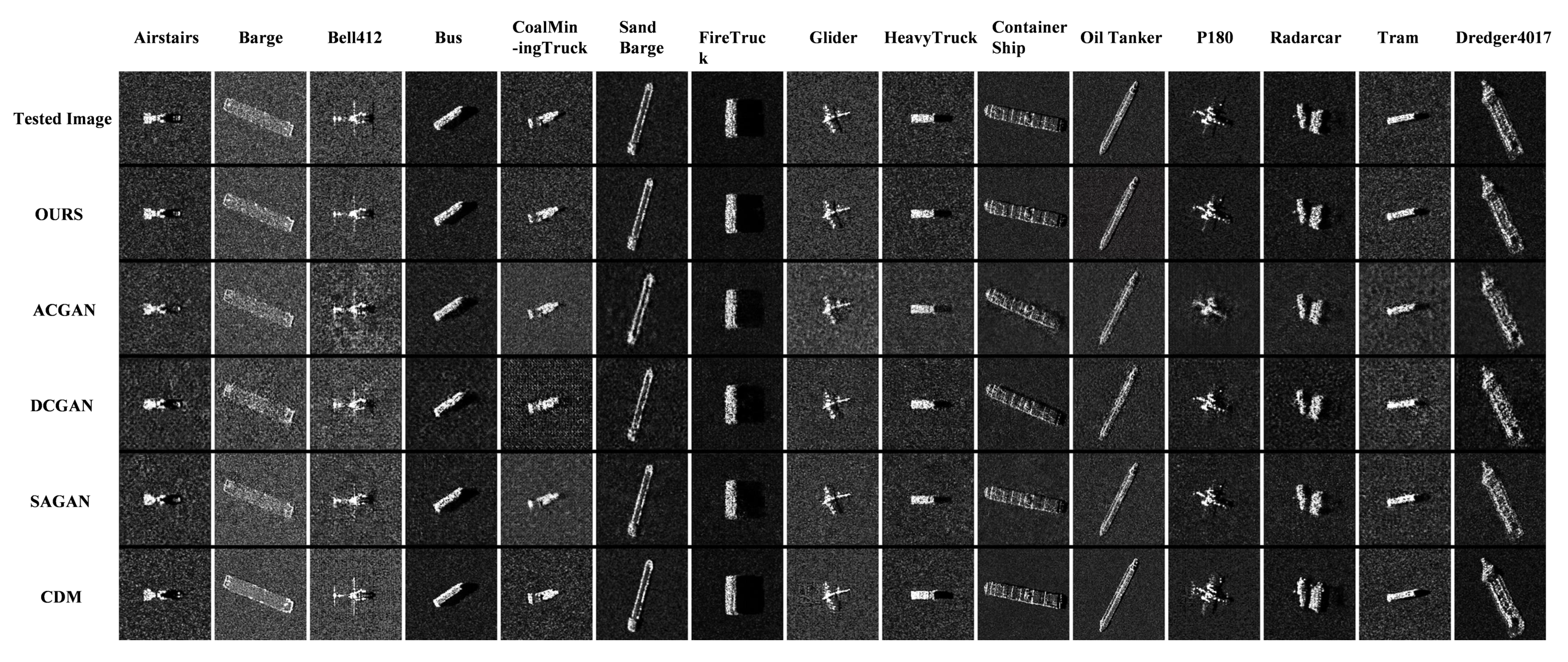
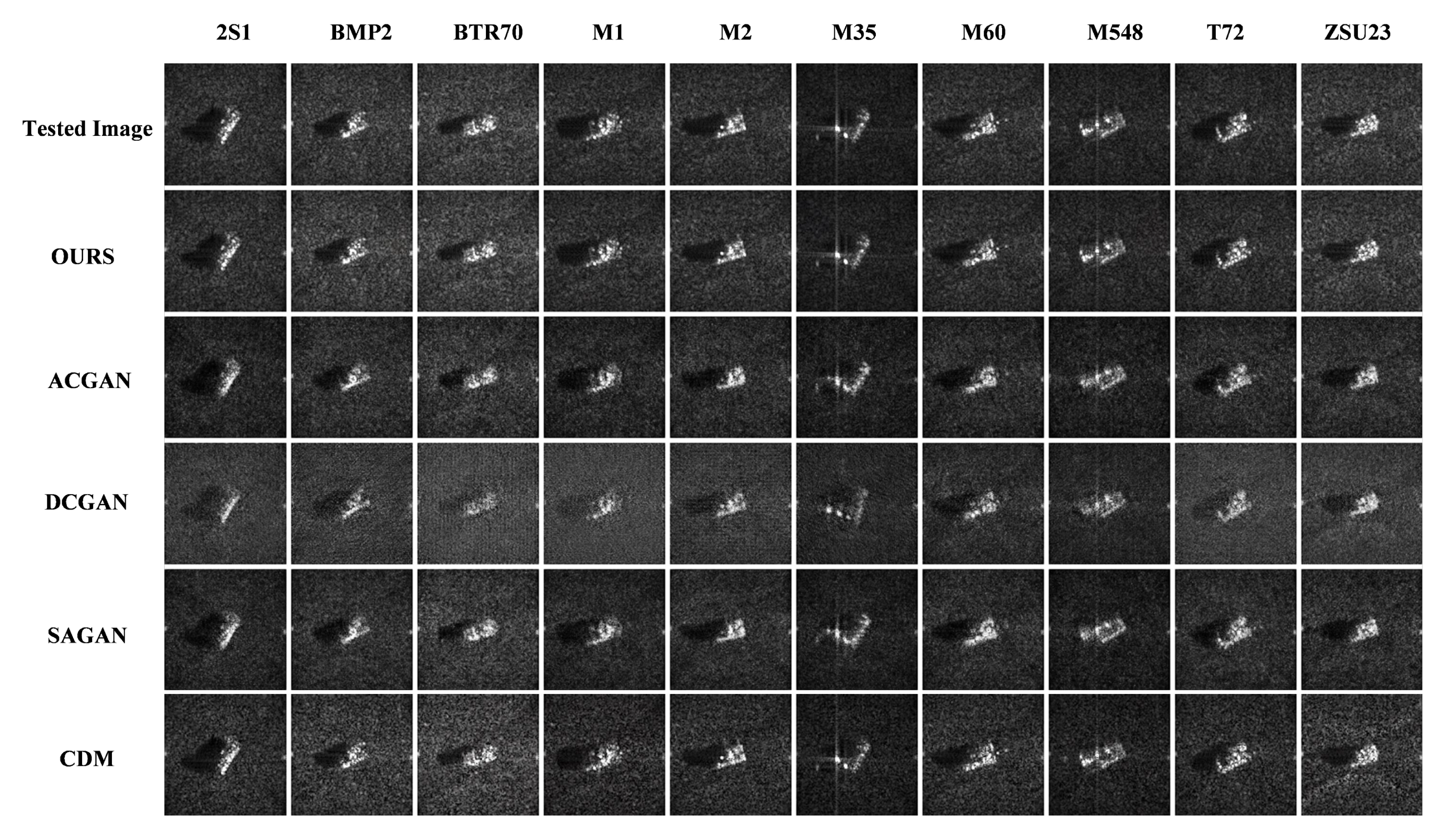
To further evaluate the effectiveness of the proposed model, we conducted comparative experiments against four widely adopted baseline methods: DCGAN, ACGAN, SAGAN and CDM (Conditional Diffusion Model). The implementations of all baseline models were reproduced from open-source code and trained using the same dataset as employed in this study. The quantitative evaluation of generated results for the training dataset angles is presented in Figure 16 and Figure 17 and

Table 5. Quantitative results for different generation methods.

Method	FID	KID	MS-SSIM	${\mathbf{PRD}}_{\mathbf{best}\_\mathbf{F}1}$	MemScore
OURS	$6.541\pm 0.123$	$0.001\pm 0.000$	$0.907\pm 0.029$	$0.875\pm 0.007$	$0.000\pm 0.000$
DCGAN	$90.927\pm 1.704$	$0.087\pm 0.003$	$0.569\pm 0.046$	$0.537\pm 0.019$	$0.000\pm 0.000$
ACGAN	$73.840\pm 1.595$	$0.062\pm 0.001$	$0.619\pm 0.063$	$0.565\pm 0.017$	$0.000\pm 0.000$
SAGAN	$68.691\pm 2.398$	$0.062\pm 0.003$	$0.658\pm 0.023$	$0.614\pm 0.016$	$0.000\pm 0.000$
CDM	$21.610\pm 0.381$	$0.004\pm 0.001$	$0.837\pm 0.019$	$0.816\pm 0.012$	$0.028\pm 0.000$

.

The quantitative results in Table 5 demonstrate that the proposed method (OURS) achieves the best overall fidelity and perceptual quality among the evaluated approaches. Our model attains a mean FID of $6.541\pm 0.123$, a KID of $0.001\pm 0.000$, and an MS-SSIM of $0.907\pm 0.029$, indicating both high realism and strong structural consistency with the real data distribution. The conventional GAN baselines perform slightly worse: DCGAN exhibits inferior performance relative to the other GAN variants (FID $90.927\pm 1.704$, KID $0.087\pm 0.003$, MS-SSIM $0.569\pm 0.046$), which manifests in a small number of instances with unclear object boundaries and irregular target geometries. ACGAN reduces FID relative to DCGAN (FID $73.840\pm 1.595$) and improves structural similarity (MS-SSIM $0.619\pm 0.063$), yet residual artifacts such as edge blurring and uneven background noise persist. The inclusion of self-attention in SAGAN further improves global texture modeling and edge delineation (FID $68.691\pm 2.398$, MS-SSIM $0.658\pm 0.023$), although SAGAN still falls short in reproducing the finest local scattering details.

Introducing a CDM (Conditional Diffusion Model) substantially narrows the gap between GAN-based generators and our approach: it attains markedly lower FID ($21.610\pm 0.381$) and KID ($0.004\pm 0.001$) than the GAN baselines, together with high MS-SSIM ($0.837\pm 0.019$) and PRD_best_f1 ($0.816\pm 0.012$), indicating improved fidelity of both global structure and local texture. Overall, while the Conditional Diffusion Model represents a substantial improvement over classic GAN architectures in capturing SAR scattering characteristics, our method still provides the most faithful and consistent synthesis according to the evaluated metrics (particularly FID and KID). The reported means and standard deviations demonstrate that these differences are stable across repeated runs.

Furthermore, given that the primary objective of this study is to address the problem of missing observation angles in the target SAR image dataset, we extend the evaluation beyond generating images at angles already included in the dataset (i.e., 10° intervals from 10° to 360°). Specifically, we interpolate intermediate angles at 5° intervals (e.g., 5°, 15°, and 355°) to assess the network’s generalization capability to untrained angles and to examine the feasibility and reliability of the generated images for dataset augmentation. Using the Oil Tanker target as a representative example, we provide a comparative analysis of images generated by different GAN-based networks at 5° increments between 10° and 90°. The interpolated angles are highlighted with red bounding boxes, and the corresponding generated results are presented in Figure 18.

The Figure 18 highlights substantial differences in the performance of various conditional generative models for interpolated angle generation. Specifically, models including DCGAN, ACGAN, and SAGAN achieve satisfactory performance when trained on discrete angles (e.g., 10°, 20°, …, 360°). The generated samples exhibit discernible boundaries and regular shapes, indicating acceptable image fidelity and diversity. However, their generation quality degrades markedly at untrained interpolated angles (e.g., 15° and 25°), where visual artifacts increase and quantitative metrics deteriorate significantly compared with the trained cases. In contrast, the proposed model consistently maintains high-quality generation even for untrained angles. StyleGAN2-ADA incorporates a mapping network combined with an angle encoder to embed angles into a continuous latent space. This design effectively conveys angular continuity, enabling the model to learn smooth relationships across adjacent observation angles and thereby significantly improving the quality of generated images for untrained interpolated angles.

4.6. SAR Target Recognition Application Evaluation

To evaluate the effectiveness of the generated multi-target, multi-angle SAR images for target recognition, the classical VGG16 network [61] is employed as the evaluation model, and experiments are conducted on two datasets. Specifically, both the self-constructed multi-target SAR dataset and the SAMPLE dataset are partitioned into a baseline dataset and a sample-augmented dataset.

To ensure a rigorous evaluation, all StyleGAN2-generated images were used exclusively for augmentation and were never included in the test baseline set. That is, the test baseline set contained no SAR images synthesized by StyleGAN2. For the self-constructed dataset, the baseline dataset consists of SAR images generated via electromagnetic scattering modeling, while the augmented dataset additionally incorporates StyleGAN2-generated SAR images at 5° intervals. For the SAMPLE dataset, SAR images acquired at 5° intervals between 10° and 79° are used to construct the baseline training and testing sets, whereas the augmented dataset is enriched with StyleGAN2-generated SAR images at 3° intervals. The detailed distribution of samples is summarized in

Table 6. Per-class sample distribution summary for the self-constructed and SAMPLE datasets.

Dataset	Classes	Samples per Class (Baseline)	Samples per Class (Augmented)	Total Samples (Baseline/Augmented)
Airstairs-Dredger4017	15	36 (uniform)	43 (uniform)	540/645
2S1-ZSU23	10	15 (uniform)	35 (uniform)	150/350

.

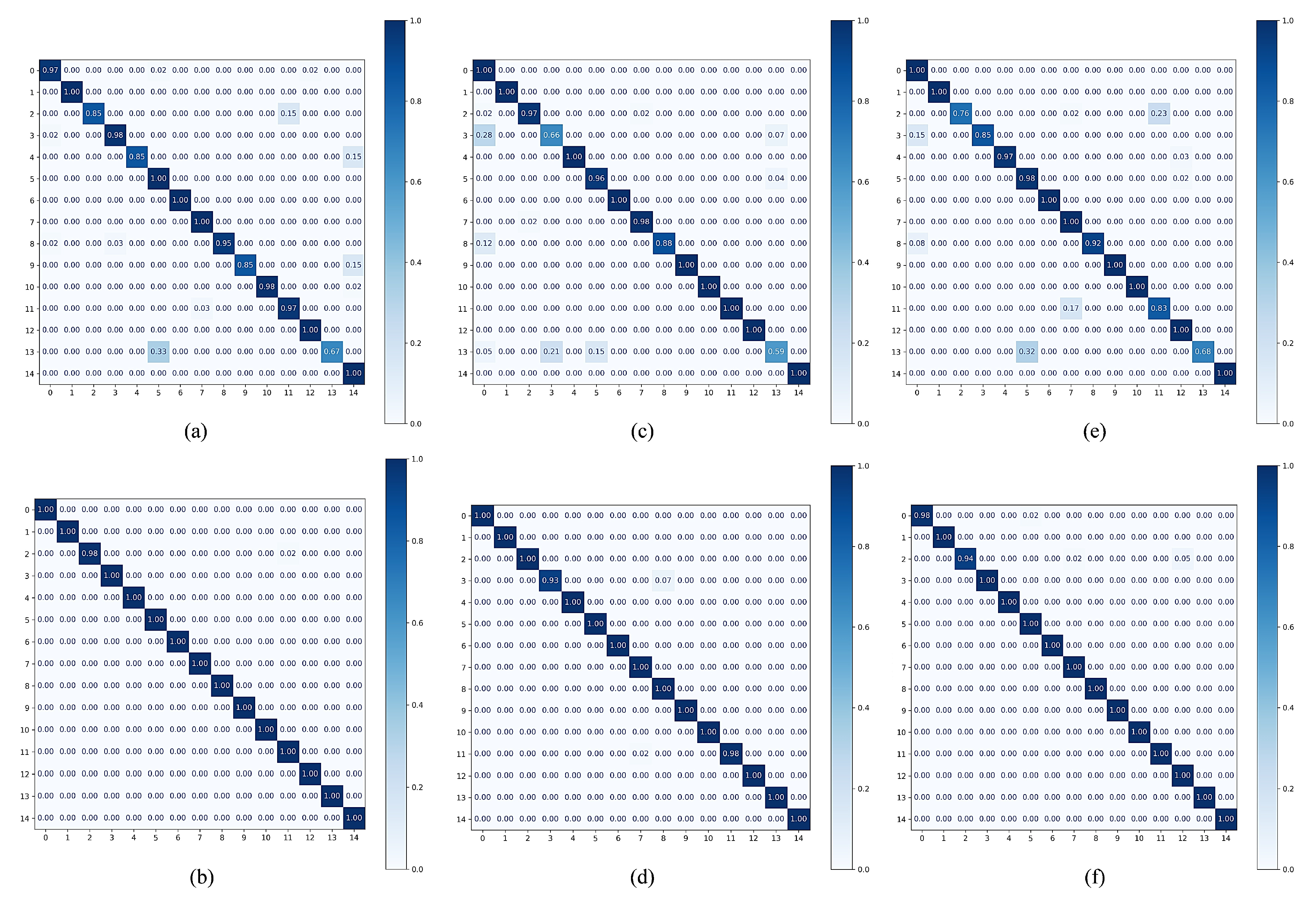
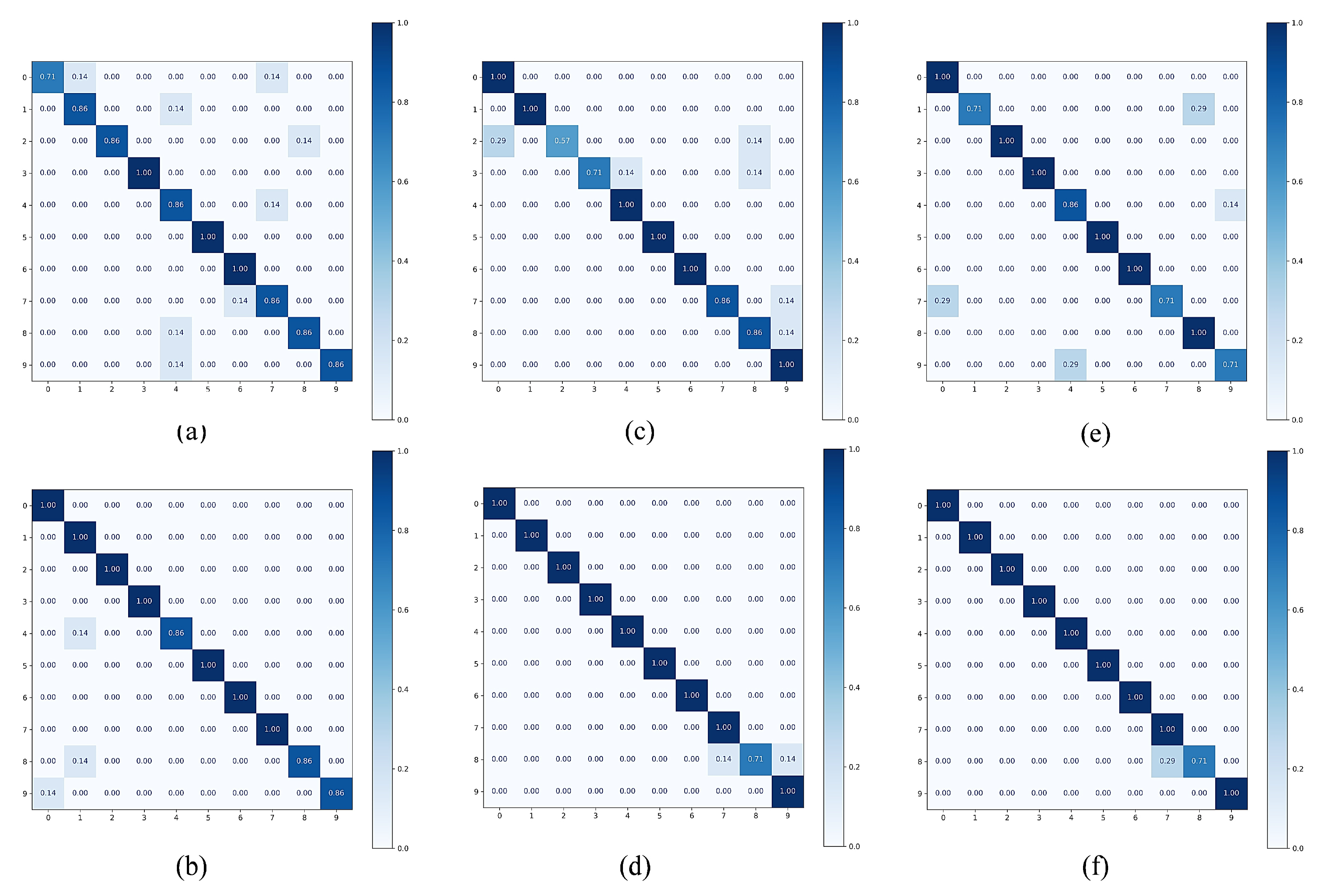
To ensure the reliability of the results, each experiment was independently repeated three times under identical hyperparameter and random seed settings to mitigate the impact of random variations. Figure 19 presents the recognition accuracy confusion matrix of the VGG16 network on the self-constructed dataset. As shown in Figure 19, average recognition accuracy is substantially improved after sample augmentation. A similar trend is observed in Figure 20, which reports the confusion matrix of VGG16 recognition on the MSTAR dataset. These results consistently confirm that the proposed image generation approach effectively enhances recognition performance by augmenting the diversity and coverage of training samples.

The experimental results for VGG16 are presented in

Table 7. Average recognition performance of VGG16 on self-constructed datasets.

Trials	Accuracy (%)	Macro-F1
	Before/After	Before/After
1	93.83/99.90	0.938/0.999
2	93.61/99.46	0.935/0.995
3	93.33/99.49	0.933/0.995
Average ± std	93.59 ± 0.25/99.62 ± 0.23	0.935 ± 0.002/0.996 ± 0.002

,

Table 8. Average recognition performance of VGG16 on the SAMPLE dataset.

Trials	Accuracy (%)	Macro-F1
	Before/After	Before/After
1	88.57/95.71	0.8858/0.9578
2	90.00/97.14	0.8956/0.9700
3	90.00/97.14	0.8986/0.9708
Average ± std	89.52 ± 0.83/96.66 ± 0.83	0.8933 ± 0.0055/0.9662 ± 0.0060

,

Table 9. Aggregated per-class F1 (mean ± std) over three trials for VGG16 on self-constructed datasets.

Class	Before Aug	After Aug	Class	Before Aug	After Aug
0	0.894 ± 0.064	0.998 ± 0.004	7	0.962 ± 0.032	0.995 ± 0.004
1	1.000 ± 0.000	1.000 ± 0.000	8	0.958 ± 0.017	0.989 ± 0.015
2	0.919 ± 0.047	0.987 ± 0.014	9	0.973 ± 0.039	1.000 ± 0.000
3	0.867 ± 0.119	0.989 ± 0.016	10	0.998 ± 0.004	1.000 ± 0.000
4	0.968 ± 0.036	1.000 ± 0.000	11	0.908 ± 0.078	0.995 ± 0.004
5	0.871 ± 0.027	0.998 ± 0.004	12	0.989 ± 0.010	0.992 ± 0.011
6	1.000 ± 0.000	1.000 ± 0.000	13	0.769 ± 0.052	1.000 ± 0.000
—			14	0.954 ± 0.065	1.000 ± 0.000

and

Table 10. Aggregated per-class F1 (mean ± std) over three trials for VGG16 on the SAMPLE dataset.

Class	Before Aug	After Aug	Class	Before Aug	After Aug
0	0.860 ± 0.021	0.978 ± 0.031	5	1.000 ± 0.000	1.000 ± 0.000
1	0.896 ± 0.074	0.958 ± 0.059	6	0.977 ± 0.032	1.000 ± 0.000
2	0.883 ± 0.115	1.000 ± 0.000	7	0.851 ± 0.052	0.936 ± 0.051
3	0.944 ± 0.080	1.000 ± 0.000	8	0.842 ± 0.033	0.863 ± 0.042
4	0.826 ± 0.078	0.974 ± 0.036	9	0.854 ± 0.064	0.952 ± 0.034

. Table 7 and Table 8 report recognition Accuracy and Macro-F1 for each trial on our self-constructed dataset and the SAMPLE dataset, respectively; Macro-F1 is computed as the unweighted mean of per-class F1 scores. Table 9 and Table 10 further list the category-wise F1 scores (mean ± std) for the respective datasets. Although Accuracy and Macro-F1 are numerically similar in our tables (Macro-F1 is reported in the 0–1 range and corresponds to the percentage values shown for Accuracy), this similarity reflects the near-uniform per-class performance and the approximately balanced test sets rather than metric redundancy. The results indicate consistent and significant enhancements in both overall and per-class performance after data augmentation. Specifically, for the self-constructed multi-target SAR dataset, the three-run average accuracy increases from 93.59% to 99.62% (an improvement of 6.03%); Macro-F1 increases from 0.935 to 0.996. For the SAMPLE dataset, accuracy improves from 89.52% to 96.66% (a gain of 7.14%); Macro-F1 increases from 0.8933 to 0.9662. These results confirm that the generated images not only conform to the true data distribution but also effectively compensate for missing observation angles through interpolation. To further demonstrate robustness, we also report per-class F1 (Table 9 and Table 10), class/angle sample balances.

5. Conclusions

In this study, multi-target and multi-angle conditional information is first processed through an angle encoder and then combined with random noise to serve as input to the StyleGAN2 framework, providing an effective approach for controllable generation of multi-view synthetic aperture radar (SAR) images. During the generation process, attention mechanisms (SimAM and IAAM) and perceptual loss are incorporated to enhance image fidelity, achieve precise angle control, and improve the network’s generalization to untrained angles.

Extensive experiments on two datasets demonstrate that the proposed method outperforms baseline approaches in structural detail, feature distribution, and stability of synthesized angles. The results further confirm that the approach effectively enhances SAR target recognition accuracy, highlighting its feasibility and robustness under limited-sample conditions.

Future work will focus on developing more efficient generation strategies and expanding SAR sample datasets to address challenges related to small sample sizes and mode collapse. This will provide a solid foundation for SAR-based target detection, recognition, and three-dimensional reconstruction, thereby facilitating broader practical applications of SAR technology. Additionally, we will focus on advancing evaluation metrics tailored for SAR images, particularly by developing Fréchet distance-based metrics grounded in ATR backbone networks.

References

1. Wang, C.; Pei, J.; Liu, X.; Huang, Y.; Yang, J. A Deep Deformable Residual Learning Network for SAR Image Segmentation. In Proceedings of the 2021 IEEE Radar Conference (RadarConf21), Atlanta, GA, USA, 7–14 May 2021; pp. 1–5. [Google Scholar]
2. Wang, C.; Pei, J.; Li, M.; Zhang, Y.; Huang, Y.; Yang, J. Parking information perception based on automotive millimeter wave SAR. In Proceedings of the 2019 IEEE Radar Conference (RadarConf), Boston, MA, USA, 22–26 April 2019; pp. 1–6. [Google Scholar]
3. Ma, L.; Liu, Y.; Zhang, X.; Ye, Y.; Yin, G.; Johnson, B.A. Deep Learning in Remote Sensing Applications: A Meta-Analysis and Review. ISPRS J. Photogramm. Remote Sens. 2019, 152, 166–177. [Google Scholar] [CrossRef]
4. Wang, C.; Xu, R.; Huang, Y.; Pei, J.; Huang, C.; Zhu, W.; Yang, J. Limited-data SAR ATR causal method via dual-invariance intervention. IEEE Trans. Geosci. Remote Sens. 2025, 63, 5203319. [Google Scholar] [CrossRef]
5. Diemunsch, J.R.; Wissinger, J. Moving and stationary target acquisition and recognition (MSTAR) model-based automatic target recognition: Search technology for a robust ATR. In Proceedings of the Algorithms for Synthetic Aperture Radar Imagery V, Orlando, FL, USA, 14–17 April 1998; SPIE: Cergy, France, 1998; Volume 3370, pp. 481–492. [Google Scholar]
6. Zheng, J.; Li, M.; Zhang, P.; Wu, Y.; Chen, H. Position-aware graph neural network for few-shot SAR target classification. IEEE J. Sel. Top. Appl. Earth Observ. Remote Sens. 2024, 17, 8028–8042. [Google Scholar] [CrossRef]
7. Sun, Z.; Leng, X.; Lei, Y.; Xiong, B.; Ji, K.; Kuang, G. BiFA-YOLO: A novel YOLO-based method for arbitrary-oriented ship detection in high-resolution SAR images. Remote Sens. 2021, 13, 4209. [Google Scholar] [CrossRef]
8. Deng, J.; Wang, W.; Zhang, H.; Zhang, T.; Zhang, J. PolSAR ship detection based on superpixel-level contrast enhancement. IEEE Geosci. Remote Sens. Lett. 2024, 21, 4008805. [Google Scholar] [CrossRef]
9. Guan, T.; Chang, S.; Deng, Y.; Xue, F.; Wang, C.; Jia, X. Oriented SAR ship detection based on edge deformable convolution and point set representation. Remote Sens. 2025, 17, 1612. [Google Scholar] [CrossRef]
10. Zheng, J.; Li, M.; Li, X.; Zhang, P.; Wu, Y. SVD-Based Feature Reconstruction Metric Network With Active Contrast Loss for Few-Shot SAR Target Recognition. IEEE J. Sel. Top. Appl. Earth Observ. Remote Sens. 2025, 18, 7391–7405. [Google Scholar] [CrossRef]
11. Zhao, Y.; Zhao, L.; Zhang, S.; Ji, K.; Kuang, G.; Liu, L. Azimuth-aware subspace classifier for few-shot class-incremental SAR ATR. IEEE Trans. Geosci. Remote Sens. 2024, 62, 5203020. [Google Scholar] [CrossRef]
12. Salcedo-Sanz, S.; Ghamisi, P.; Piles, M.; Werner, M.; Cuadra, L.; Moreno-Martínez, A.; Izquierdo-Verdiguier, E.; Muñoz-Marí, J.; Mosavi, A.; Camps-Valls, G. Machine learning information fusion in Earth observation: A comprehensive review of methods, applications and data sources. Inf. Fusion 2020, 63, 256–272. [Google Scholar] [CrossRef]
13. Sun, X.; Wang, B.; Wang, Z.; Li, H.; Li, H.; Fu, K. Research Progress on Few-Shot Learning for Remote Sensing Image Interpretation. IEEE J. Sel. Top. Appl. Earth Obs. Remote Sens. 2021, 14, 2387–2402. [Google Scholar] [CrossRef]
14. Huang, Z.; Pan, Z.; Lei, B. What, Where, and How to Transfer in SAR Target Recognition Based on Deep CNNs. IEEE Trans. Geosci. Remote Sens. 2020, 58, 2324–2336. [Google Scholar] [CrossRef]
15. Hu, X.; Zhang, P.; Ban, Y.; Rahnemoonfar, M. GAN-based SAR and optical image translation for wildfire impact assessment using multi-source remote sensing data. Remote Sens. Environ. 2023, 289, 113522. [Google Scholar] [CrossRef]
16. Li, J.; Yu, Z.; Yu, L.; Cheng, P.; Chen, J.; Chi, C. A Comprehensive Survey on SAR ATR in Deep-Learning Era. Remote Sens. 2023, 15, 1454. [Google Scholar] [CrossRef]
17. Mumuni, A.; Mumuni, F. Data Augmentation: A Comprehensive Survey of Modern Approaches. Array 2022, 16, 100258. [Google Scholar] [CrossRef]
18. Zhang, P.; Xu, H.; Tian, T.; Gao, P.; Li, L.; Zhao, T.; Zhang, N.; Tian, J. SEFEPNet: Scale Expansion and Feature Enhancement Pyramid Network for SAR Aircraft Detection With Small Sample Dataset. IEEE J. Sel. Top. Appl. Earth Observ. Remote Sens. 2022, 15, 3365–3375. [Google Scholar] [CrossRef]
19. Wang, C.; Pei, J.; Liu, X.; Huang, Y.; Mao, D.; Zhang, Y.; Yang, J. SAR target image generation method using azimuth-controllable generative adversarial network. IEEE J. Sel. Top. Appl. Earth Observ. Remote Sens. 2022, 15, 9381–9397. [Google Scholar] [CrossRef]
20. Zhang, H.; Wang, W.; Deng, J.; Guo, Y.; Liu, S.; Zhang, J. MASFF-Net: Multiazimuth scattering feature fusion network for SAR target recognition. IEEE J. Sel. Top. Appl. Earth Observ. Remote Sens. 2025, 18, 19425–19440. [Google Scholar] [CrossRef]
21. Zhao, P.; Huang, L.; Xin, Y.; Guo, J.; Pan, Z. Multi-aspect SAR target recognition based on prototypical network with a small number of training samples. Sensors 2021, 21, 4333. [Google Scholar] [CrossRef]
22. Dostalova, A.; Navacchi, C.; Greimeister-Pfeil, I.; Small, D.; Wagner, W. The Effects of Radiometric Terrain Flattening on SAR-Based Forest Mapping and Classification. Remote Sens. Lett. 2022, 13, 855–864. [Google Scholar] [CrossRef]
23. Malmgren-Hansen, D.; Kusk, A.; Dall, J.; Nielsen, A.A.; Engholm, R.; Skriver, H. Improving SAR Automatic Target Recognition Models with Transfer Learning From Simulated Data. IEEE Geosci. Remote Sens. Lett. 2017, 14, 1484–1488. [Google Scholar] [CrossRef]
24. Song, Q.; Xu, F.; Zhu, X.X.; Jin, Y.-Q. Learning to Generate SAR Images with Adversarial Autoencoder. IEEE Trans. Geosci. Remote Sens. 2022, 60, 5210015. [Google Scholar] [CrossRef]
25. Zhang, M.; Cui, Z.; Wang, X.; Cao, Z. Data augmentation method of SAR image dataset. In Proceedings of the IGARSS 2018—2018 IEEE International Geoscience and Remote Sensing Symposium, Valencia, Spain, 22–27 July 2018; pp. 5292–5295. [Google Scholar]
26. Cui, Z.; Zhang, M.; Cao, Z.; Cao, C. Image data augmentation for SAR sensor via generative adversarial nets. IEEE Access 2019, 7, 42255–42268. [Google Scholar] [CrossRef]
27. Ruyi, W.; Zhang, H.; Han, B.; Zhang, Y.; Guo, J.; Hong, W.; Sun, W.; Hu, W. Multiangle SAR dataset construction of aircraft targets based on angle interpolation simulation. J. Radar 2022, 11, 637–651. [Google Scholar]
28. Zeng, Z.; Tan, X.; Zhang, X.; Huang, Y.; Wan, J.; Chen, Z. ATGAN: A SAR target image generation method for automatic target recognition. IEEE J. Sel. Top. Appl. Earth Observ. Remote Sens. 2024, 17, 6290–6307. [Google Scholar] [CrossRef]
29. Karras, T.; Aittala, M.; Hellsten, J.; Laine, S.; Lehtinen, J.; Aila, T. Training generative adversarial networks with limited data. Adv. Neural Inf. Process. Syst. 2020, 33, 12104–12114. [Google Scholar]
30. Ahmadibeni, A.; Borooshak, L.; Jones, B.; Shirkhodaie, A. Aerial and ground vehicles synthetic SAR dataset generation for automatic target recognition. Algorithms Synth. Aperture Radar Imag. XXVII 2020, 11393, 96–107. [Google Scholar]
31. Leng, X.; Ji, K.; Kuang, G. Ship detection from raw SAR echo data. IEEE Trans. Geosci. Remote Sens. 2023, 61, 5207811. [Google Scholar] [CrossRef]
32. Li, G.; Yang, X.; Zhang, Y.; Liu, B.; Ren, H. Three-Dimensional Reconstruction of Multi-View SAR Ship Targets Based on Semantic Information. In Proceedings of the IGARSS 2024—2024 IEEE International Geoscience and Remote Sensing Symposium, Athens, Greece, 7–12 July 2024; pp. 9794–9797. [Google Scholar]
33. Eker, T.A.; Heslinga, F.G.; Ballan, L.; den Hollander, R.J.M.; Schutte, K. The effect of simulation variety on a deep learning-based military vehicle detector. In Artificial Intelligence for Security and Defence Applications; SPIE: Cergy, France, 2023; Volume 12742, pp. 183–196. [Google Scholar]
34. Chiang, C.-Y.; Chen, K.-S.; Yang, Y.; Zhang, Y.; Zhang, T. SAR image simulation of complex target including multiple scattering. Remote Sens. 2021, 13, 4854. [Google Scholar] [CrossRef]
35. Ghanbarabad, S.J.H.; Asadi, Z.; Mohtashami, V. Adaptive supersampling of rays for accurate calculation of physical optics scattering from parametric surfaces. IEEE Antennas Wirel. Propag. Lett. 2018, 17, 960–963. [Google Scholar] [CrossRef]
36. Shan, J.; Xu, X. Multipath Model Enhanced SBR Technique for Prediction of Near-Field EM Scattering from Objects on Rough Surfaces. IEEE Trans. Antennas Propag. 2025, 73, 539–553. [Google Scholar] [CrossRef]
37. Feng, T.-T.; Guo, L.-X. An improved ray-tracing algorithm for SBR-based EM scattering computation of electrically large targets. IEEE Antennas Wireless Propag. Lett. 2021, 20, 818–822. [Google Scholar] [CrossRef]
38. Karam, M.A.; McDonough, R.S. Analytic models for bistatic scattering from a randomly rough surface with complex relative permittivity. ITU J. ICT Discov. 2019, 2, 7. [Google Scholar] [PubMed]
39. Yahia, O.; Guida, R.; Iervolino, P. Novel weight-based approach for soil moisture content estimation via synthetic aperture radar, multispectral and thermal infrared data fusion. Sensors 2021, 21, 3457. [Google Scholar] [CrossRef] [PubMed]
40. Yun, Z.; Iskander, M.F. Radio Propagation Modeling and Simulation Using Ray Tracing. In The Advancing World of Applied Electromagnetics: In Honor and Appreciation of Magdy Fahmy Iskander; Springer: Cham, Switzerland, 2024; pp. 251–279. [Google Scholar]
41. Wu, K.; Jin, G.; Xiong, X.; Zhang, H.; Wang, L. Fast SAR image simulation based on echo matrix cell algorithm including multiple scattering. Remote Sens. 2023, 15, 3637. [Google Scholar] [CrossRef]
42. Danby, J.M.A. Fundamentals of Celestial Mechanics, 2nd ed.; Willmann-Bell, Inc.: Richmond, VA, USA, 1988; Chapter 11; ISBN 978-0-943396-20-0. [Google Scholar]
43. Li, H.; An, J.; Jiang, X. Accurate Range Modeling for High-Resolution Spaceborne Synthetic Aperture Radar. Sensors 2024, 24, 3119. [Google Scholar] [CrossRef]
44. Bamler, R. A comparison of range-Doppler and wavenumber domain SAR focusing algorithms. IEEE Trans. Geosci. Remote Sens. 2002, 30, 706–713. [Google Scholar] [CrossRef]
45. Raney, R.K.; Runge, H.; Bamler, R.; Cumming, I.G.; Wong, F.H. Precision SAR processing using chirp scaling. IEEE Trans. Geosci. Remote Sens. 2002, 32, 786–799. [Google Scholar] [CrossRef]
46. Rodríguez, P.; Bautista, M.A.; Gonzalez, J.; Escalera, S. Beyond one-hot encoding: Lower dimensional target embedding. Image Vis. Comput. 2018, 75, 21–31. [Google Scholar] [CrossRef]
47. Sun, Y.; Zheng, J.; Zhao, H.; Zhou, H.; Li, J.; Li, F.; Xiong, Z.; Liu, J.; Li, Y. Modifying the one-hot encoding technique can enhance the adversarial robustness of the visual model for symbol recognition. Expert Syst. Appl. 2024, 250, 123751. [Google Scholar] [CrossRef]
48. Yang, L.; Zhang, R.-Y.; Li, L.; Xie, X. Simam: A simple, parameter-free attention module for convolutional neural networks. In Proceedings of the 38th International Conference on Machine Learning, PMLR, Virtual, 18–24 July 2021; pp. 11863–11874. [Google Scholar]
49. Hu, J.; Shen, L.; Sun, G. Squeeze-and-excitation networks. In Proceedings of the 2018 IEEE/CVF Conference on Computer Vision and Pattern Recognition, Salt Lake City, UT, USA, 18–23 June 2018; pp. 7132–7141. [Google Scholar]
50. Woo, S.; Park, J.; Lee, J.-Y.; Kweon, I.S. CBAM: Convolutional block attention module. In Proceedings of the Computer Vision—ECCV 2018: 15th European Conference, Munich, Germany, 8–14 September 2018; pp. 3–19. [Google Scholar]
51. Anggreyni, D.P.; Indriatmoko; Arymurthy, A.M.; Setiyoko, A. Enhancing Remote Sensing Image Quality through Data Fusion and Synthetic Aperture Radar (SAR): A Comparative Analysis of CNN, Lightweight ConvNet, and VGG16 Models. J. Online Inform. 2024, 9, 210–218. [Google Scholar] [CrossRef]
52. Tao, J.; Gu, Y.; Sun, J.; Bie, Y.; Wang, H. Research on VGG16 Convolutional Neural Network Feature Classification Algorithm Based on Transfer Learning. In Proceedings of the 2021 2nd China International SAR Symposium (CISS), Shanghai, China, 3–5 November 2021; IEEE: Beijing, China, 2021; pp. 1–3. [Google Scholar]
53. Karras, T.; Laine, S.; Aittala, M.; Hellsten, J.; Lehtinen, J.; Aila, T. Analyzing and improving the image quality of StyleGAN. In Proceedings of the 2020 IEEE/CVF Conference on Computer Vision and Pattern Recognition (CVPR), Seattle, WA, USA, 13–19 June 2020; pp. 8110–8119. [Google Scholar]
54. Lewis, B.; Scarnati, T.; Sudkamp, E.; Nehrbass, J.; Rosencrantz, S.; Zelnio, E. A SAR dataset for ATR development: The Synthetic and Measured Paired Labeled Experiment (SAMPLE). In Algorithms for Synthetic Aperture Radar Imagery XXVI; SPIE: Cergy, France, 2019; Volume 10987, pp. 39–54. [Google Scholar]
55. Yu, Q.; Wang, N.; Tang, H.; Zhang, J.; Xu, R.; Liu, L. In Situ Root Dataset Expansion Strategy Based on an Improved CycleGAN Generator. Plant Phenom. 2024, 6, 0148. [Google Scholar] [CrossRef] [PubMed]
56. Wang, Z.; Simoncelli, E.P.; Bovik, A.C. Multiscale Structural Similarity for Image Quality Assessment. Proc. Asilomar Conf. Signals Syst. Comput. 2003, 2, 1398–1402. [Google Scholar] [CrossRef]
57. Sun, Z.; Leng, X.; Zhang, X.; Zhou, Z.; Xiong, B.; Ji, K.; Kuang, G. Arbitrary-Direction SAR Ship Detection Method for Multiscale Imbalance. IEEE Trans. Geosci. Remote Sens. 2025, 63, 5208921. [Google Scholar] [CrossRef]
58. van den Burg, G.; Williams, C. On Memorization in Probabilistic Deep Generative Models. Adv. Neural Inf. Process. Syst. 2021, 34, 27916–27928. [Google Scholar]
59. Maaten, L.v.d.; Hinton, G. Visualizing data using t-SNE. J. Mach. Learn. Res. 2008, 9, 2579–2605. [Google Scholar]
60. McInnes, L.; Healy, J.; Melville, J. Umap: Uniform manifold approximation and projection for dimension reduction. arXiv 2018, arXiv:1802.03426. [Google Scholar]
61. Simonyan, K.; Zisserman, A. Very deep convolutional networks for large-scale image recognition. arXiv 2014, arXiv:1409.1556. [Google Scholar]
Figure 1. Comparison of the dataset target optical image and its corresponding 3D model.The first row is the target optical image, and the second row is the target 3D model. (a) Airstairs; (b) Barge; (c) Bell412; (d) Bus; (e) Coal Mining Truck; (f) Sand Barge; (g) Fire Truck; (h) Glider; (i) Heavy Truck; (j) Container Ship; (k) Oil Tanker; (l) P180; (m) Radarcar; (n) Tram; (o) Dredger4017.
Remotesensing 17 03478 g001
Figure 2. Ray tracing method. (a) Coordinate system setup diagram, (b) Ray tracing schematic.
Remotesensing 17 03478 g002
Figure 3. Dataset 3D models and their corresponding SAR images. The first row is the target 3D model, and the second row is the target SAR image. (a) Airstairs; (b) Barge; (c) Bell412; (d) Bus; (e) Coal Mining Truck; (f) Sand Barge; (g) Fire Truck; (h) Glider; (i) Heavy Truck; (j) Container Ship; (k) Oil Tanker; (l) P180; (m) Radarcar; (n) Tram; (o) Dredger4017.
Remotesensing 17 03478 g003
Figure 4. Network framework (Dataset → Mapping/Embedding → Synthesis).
Remotesensing 17 03478 g004
Figure 5. Generator (mapping, AngleEncoder, IAAM, synthesis).
Remotesensing 17 03478 g005
Figure 6. Discriminator (conditional mapping + multi-scale + minibatch stats).
Remotesensing 17 03478 g006
Figure 7. Angle encoder.
Remotesensing 17 03478 g007
Figure 8. Block diagrams of SimAM and IAAM attention modules. (a) SimAM attention module, (b) IAAM attention module.
Remotesensing 17 03478 g008
Figure 9. Comparison of the optical and SAR images of the targets in the self-constructed multi-target multi-angle SAR dataset. The first row shows the multi-target optical images, and the second row shows the corresponding SAR images of the targets. Each column represents a different target type. (a) Airstairs; (b) Barge; (c) Bell412; (d) Bus; (e) Coal Mining Truck; (f) Sand Barge; (g) Fire Truck; (h) Glider; (i) Heavy Truck; (j) Container Ship; (k) Oil Tanker; (l) P180; (m) Radarcar; (n) Tram; (o) Dredger4017.
Remotesensing 17 03478 g009
Figure 10. Comparison of optical and corresponding SAR images of targets in the SMPLE dataset. The first row shows the optical images of multiple targets, and the second row shows the corresponding SAR images of the targets. Each column represents a different target type. (a) 2S1; (b) BMP2; (c) BTR70; (d) M1; (e) M2; (f) M35; (g) M60; (h) M548; (i) T72; (j) ZSU23.
Remotesensing 17 03478 g010
Figure 11. Image generation for 15 types of targets: 0° to 355°, captured every 5°.
Remotesensing 17 03478 g011
Figure 12. Image generation for 10 types of targets: 10° to 75°, captured every 5°.
Remotesensing 17 03478 g012
Figure 13. Training FID (a) and KID (b) curves for each ablation model (horizontal axis: training scale Kimg; vertical axis: FID/KID). The six compared models are M1–M6 with the following mapping: M1 (Baseline—gray), M2 (Baseline + AngleEncoder—blue), M3 (Baseline + AngleEncoder + IAAM—green), M4 (Baseline + AngleEncoder + IAAM + Perceptual Loss—yellow), M5 (Baseline + SimAM + Perceptual Loss—purple), and M6 (Full model—red).
Remotesensing 17 03478 g013
Figure 14. Visualization of the self-constructed multi-target SAR dataset. (a) t-SNE embedding based on target categories; (b) UMAP embedding in the single-point mode; (c) UMAP embedding in the ring-cluster mode.
Remotesensing 17 03478 g014
Figure 15. Visualization of the SAMPLE dataset. (a) t-SNE embedding colored by target category; (b) UMAP embedding in the single-point pattern; (c) UMAP embedding in the ring-shaped cluster pattern.
Remotesensing 17 03478 g015
Figure 16. Comparison of image generation by different methods based on a self-constructed dataset.
Remotesensing 17 03478 g016
Figure 17. Comparison of image generation by different methods based on the SAMPLE dataset.
Remotesensing 17 03478 g017
Figure 18. Comparison of untrained angle results from 10 to 90 degrees generated by Oil Tanker based on different methods.
Remotesensing 17 03478 g018
Figure 19. Confusion matrices of VGG16 on the self-constructed dataset. Panels (af) display the results of three experiments: (a,b) for the first experiment, (c,d) for the second, and (e,f) for the third, with each pair comparing the baseline dataset and the sample-augmented dataset.
Remotesensing 17 03478 g019
Figure 20. Confusion matrices of VGG16 on the SAMPLE dataset. Panels (af) display the results of three experiments: (a,b) for the first experiment, (c,d) for the second, and (e,f) for the third, with each pair comparing the baseline dataset and the sample-augmented dataset.
Remotesensing 17 03478 g020