Enhanced Bathymetric Inversion for Tectonic Features via Multi-Gravity-Component DenseNet: A Case Study of Rift Identification in the South China Sea

Highlights

What are the main findings?

• We develop a multi-gravity-component fusion model based on an improved DenseNet architecture, which significantly outperforms GEBCO_2024, SRTM15+, and Topo_27.1.
• Removing vertical deflection components (ξ, η) would increase bathymetric prediction errors more significantly than the exclusion of other gravity components.

What is the implication of the main finding?

• The proposed framework enables high-resolution modeling of complex tectonic features such as rifts.
• Our proposed adaptive transition layers and curvature stratification together enhance high-frequency tectonic features’ preservation and terrain generalization.

Abstract

Submarine rift systems represent critical tectonic features whose accurate bathymetric characterization remains challenging yet essential for understanding plate boundary dynamics. However, traditional bathymetric inversion methods based on altimetric gravity data exhibit poor performance in resolving rift and steep-slope terrains. To address this limitation and enhance accuracy in complex topographic regions, we propose a multi-gravity-component fusion framework based on an improved DenseNet architecture. By integrating shipborne bathymetry, gravity anomaly (GA), vertical gravity gradient (VGG), vertical deflection components (meridian component ξ and prime vertical component η), and GEBCO_2024, we construct a 16 × 16 × 9 input tensor. The model incorporates adaptive transition layers to preserve fine-scale tectonic features and curvature-based stratification to balance learning across diverse terrains. Validation using 43,035 independent points yields an RMSE of 84.75 m, representing a 47.6% reduction relative to GEBCO_2024. Crucially, in the identified rift targets, errors decreased by 69.3–87.1%. Ablation studies reveal that vertical deflection components (ξ, η) dominate the physical constraints, with their removal increasing the RMSE by 91.08 m (a 107.5% increase relative to the baseline error). Architectural innovations and stratification reduce steep-slope RMSE by 6.1%. These results validate the efficacy of directional gravity derivatives for tectonic feature inversion and demonstrate significant potential for application to mid-ocean ridge systems.

1. Introduction

High-precision seafloor topographic models are essential for marine geological research, resource exploration, ocean engineering [1,2], tectonic feature studies (e.g., rift systems and fault zones), as well as practical applications including deep-sea mining, carbon sequestration site selection, and submarine navigation safety assessments [3,4,5,6,7,8]. However, existing models exhibit significant limitations in spatial resolution and accuracy within tectonically active regions characterized by dramatic topographic variations, such as the seamounts groups and associated rift systems in the South China Sea.

Traditional bathymetric inversion methods, including the Gravity–Geologic Method (GGM) [1,9,10,11,12,13,14], the admittance method [15,16], the Smith and Sandwell (S&S) method [17], and the least-squares collocation [18,19], have achieved foundational success. Critically, these methods predominantly rely on a linear gravity–topography relationship derived from approximations of the Parker formula [20]. This linear assumption leads to significant accuracy degradation in complex tectonic terrains such as rifts and seamounts due to the neglect of nonlinear coupling effects [21]. The nonlinearity becomes particularly significant for high-relief features. Although inversion in shallow waters is also limited by factors like the proximity to the continental signal, the inherent nonlinearity of the gravity–topography relationship remains a fundamental challenge for traditional methods across various depth regimes [20]. To address this question, modifications incorporating nonlinear terms have been explored. For instance, iterative inversion methods have been employed to solve higher-order terms in the Parker series expansion, improving topographic expression [22]. Simulated annealing algorithms have been used to establish nonlinear mappings, particularly utilizing vertical gravity gradient anomalies [23]. Adaptive nonlinear iterative methods have also been developed, demonstrating significant improvements by quantifying and mitigating various error sources [24]. Physical model-driven approaches such as the Enhanced Gravity–Geologic Method (EGGM) leverage equivalent mass line approximations to account for the nonlinear gravitational effects of the surrounding topography, achieving 13.73% accuracy gains in complex regions like the Sea of Japan [25]. However, these nonlinear approaches often suffer from high computational complexity, sensitivity to initial parameters, and challenges in handling multi-source data integration, hindering their robust application to fine-scale tectonic features like rift boundaries. Consequently, there remains an urgent need to develop efficient and robust nonlinear modeling methods to overcome the inversion bottleneck for complex seafloor topography.

In recent years, deep learning has emerged as a significant paradigm for nonlinear inversion, demonstrating notable advantages in computational efficiency and flexibility. With the application of deep learning models, the research focus has progressively shifted towards the fusion of multi-source geodetic data and efficient feature extraction. Sun et al. [26] implemented the joint modeling of gravity anomaly (GA) and vertical gravity gradient (VGG) using a parallel-linked backpropagation (BP) network model. Their results showed a 19% accuracy improvement over GGM models in the Mariana Trench region, with approximately 90% of errors constrained within ±100 m. Dechao An et al. [27] and Annan et al. [28] established convolutional neural network (CNN) models to directly fuse raw vertical deflection components (meridian component ξ and prime vertical component η) with GA/VGG data. Experimental findings indicated that the predicted bathymetry accuracy surpassed both traditional methods and benchmark models like GEBCO and Topo. Their work further confirmed that the predictive accuracy achieved by combining all three gravity data types was superior to that obtained using any one or two types in combination. Zhou et al. [2,29,30] enhanced bathymetry prediction accuracy by introducing a multi-source differential strategy (e.g., gridded differences in longitude/latitude, reference depths, slopes, vertical deflection components, GA, VGG, and mean dynamic topography). This approach, implemented via a multilayer perceptron (MLP) network model, achieved breakthroughs in accuracy both regionally (e.g., the Caribbean Sea) [29,30] and globally (SDUST2023BCO model) [2]. Nevertheless, while one model may exhibit the highest overall accuracy, it may not be optimal in specific localized areas [27]. Furthermore, performance validation regarding the identification of specific linear tectonic structures, such as rifts, particularly in topographically complex regions, remains lacking.

In this study, we propose a multi-source fusion inversion framework based on an improved Densely Connected Convolutional Network (DenseNet) architecture. This framework integrates shipborne soundings, multiple gravity field components (GA, VGG, ξ, η), spatial position encoding, and a reference model (GEBCO_2024) into a structured input tensor. It incorporates architectural innovations (adaptive transition layers) to preserve fine-scale features and a novel curvature-based stratification strategy to balance learning across diverse terrain complexities. The framework specifically aims to: (1) quantitatively assess global and rift-specific inversion accuracy in the South China Sea study area; (2) elucidate the constraining mechanisms of different marine gravity field components, particularly for rift structures; and (3) advance methodologies for high-resolution modeling of complex deep-sea topography.

2. Materials and Methods

2.1. Study Area and Data

This study focuses on the seamounts group region in the central South China Sea (110°E–118°E, 10°N–18°N). Located within an active collision zone between the Eurasian and Philippine Sea plates, this region exhibits intense tectonic activity and complex geomorphology, featuring N–S trending rifts (3–7 km wide, 200–500 m deep) coupled with isolated seamounts (1000–2000 m high) [31,32] (Figure 1). This complexity makes it an ideal experimental site for validating high-precision seafloor topographic modeling methods.

Shipborne bathymetry data were sourced from the National Oceanic and Atmospheric Administration (NOAA) National Centers for Environmental Information (NCEI) (https://www.ncei.noaa.gov/maps/trackline-geophysics/, accessed on 1 August 2025), encompassing 55 shipborne single-beam survey tracks totaling 222,910 soundings within the study area. To ensure data quality, the 3σ criterion was applied for outlier detection and removal. The procedure involved calculating the absolute depth difference between each sounding and its nearest neighbor within the GEBCO_2024 grid, computing the mean (μ) and standard deviation (σ) of all differences, and eliminating points where the difference exceeded $\mathsf{\mu }+\left|3\mathsf{\sigma }\right|$. This process removed 7739 outliers (3.47% rejection rate), leaving 215,171 high-quality soundings for model training and validation. The maximum measured depth was 4992.7 m, and the average depth was 3327.7 m.

Vertical gravity gradient (VGG), gravity anomaly (GA), and vertical deflection (meridian component ξ and prime vertical component η) data from the Scripps Institution of Oceanography (SIO) V32.1 dataset (https://topex.ucsd.edu/pub/global_grav_1min/, accessed on 27 March 2025) were utilized. The original spatial resolution of the data is 1 arc-min, which was resampled to a grid resolution of 15 arc-seconds. These components provided crucial geophysical field constraints for the model.

Three benchmark datasets are utilized. The GEBCO_2024 model [33], released July 2024, jointly published by the International Hydrographic Organization (IHO) and the Intergovernmental Oceanographic Commission (IOC) of the United Nations Educational, Scientific and Cultural Organization (UNESCO), can be downloaded at https://www.gebco.net/data-products-gridded-bathymetry-data/gebco2024-grid (accessed on 25 June 2025). This model, with a 15 arc-second resolution, was used both to construct input features and as a core validation baseline for prediction accuracy. The SRTM15+ V2.7 model [34], delivers 15 arc-second mid-latitude coverage (81°S–81°N) from multi-satellite altimetry, and is available at https://topex.ucsd.edu/WWW_html/srtm15_plus.html (accessed on 25 June 2025). The Topo_27.1 model ([8]), released by the SIO in 2025, establishes a 30 arc-second global standardization baseline (90°N–90°S), and can be downloaded from https://topex.ucsd.edu/pub/global_topo_1min/ (accessed on 27 June 2025). The SRTM15+ model and Topo_27.1 models serve as independent references for marine accuracy assessments.

2.2. Methods

2.2.1. Multi-Source Data Fusion and Feature Tensor Construction

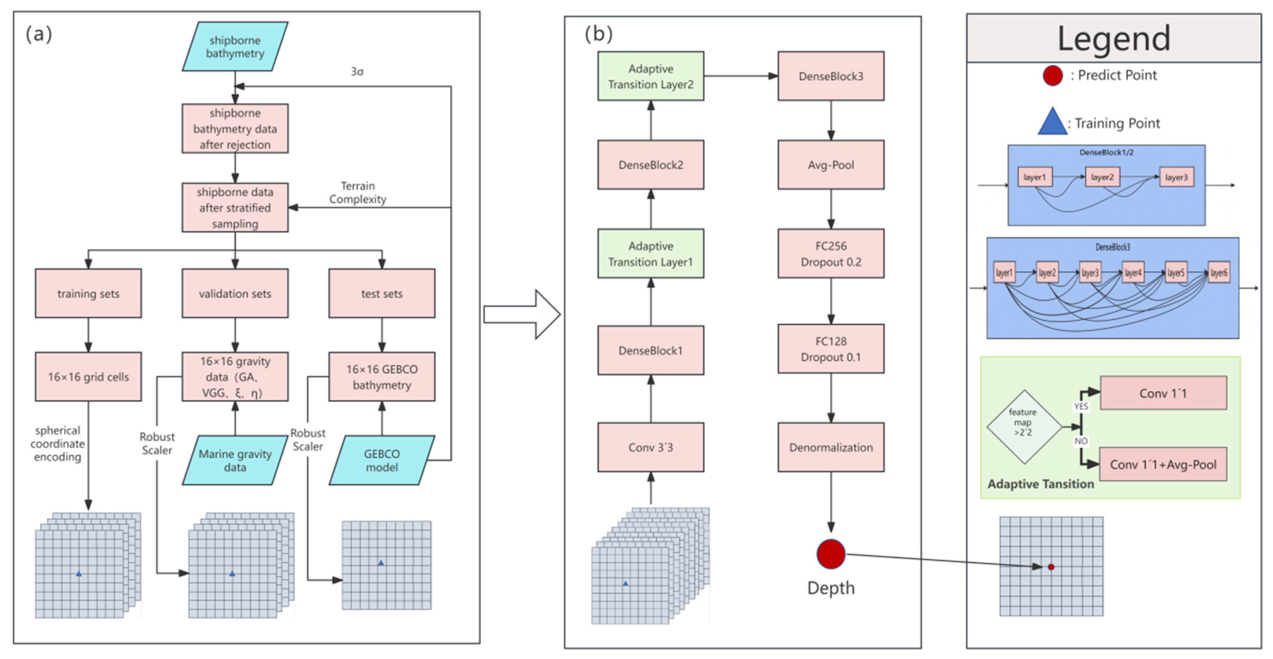
Leveraging the established physical correlation between seafloor topography and gravity field data [35], we constructed a fused multi-source input feature tensor and used shipborne soundings as control points. For each point, multi-source information from the surrounding 16 × 16 grid cells (covering approximately 7.4 km × 7.4 km) was extracted to form a three-dimensional input tensor with dimensions 16 × 16 × 9 (Figure 2). The nine channels comprised: Gravity Field Features (4 channels): VGG, GA, ξ, and η; Reference Depth (1 channel): H_ref, derived from the GEBCO_2024 model, providing baseline elevation reference; and Spatial Position Encoding (4 channels): sin(λ), cos(λ), sin(φ), cos(φ) (where λ is longitude and φ is latitude), embedding geographical location information. Unlike the RobustScaler applied to other features for numerical standardization, this encoding transforms the absolute coordinates into a continuous representation that better preserves relative spatial proximity, thereby facilitating the model’s ability to learn location-dependent patterns. To mitigate the impact of differing physical units and enhance model robustness, input data are standardized using RobustScaler (based on median and interquartile range), resulting in the normalized input tensor $\mathrm{X}\in {\mathrm{R}}^{16 \times 16 \times 9}$.

2.2.2. Data Stratification Based on Terrain Complexity

To improve the model’s generalization capability across diverse geomorphologies, the study area is stratified based on terrain complexity [36] using the curvature feature matrix |C| computed from the GEBCO_2024 model. The curvature matrix |C| is calculated as follows:

$$\mathrm{C}={\displaystyle \frac{{\partial }^2\mathrm{z}}{\partial {\mathrm{x}}^2}}+{\displaystyle \frac{{\partial }^2\mathrm{z}}{\partial {\mathrm{y}}^2}}$$

(1)

where z represents terrain elevation, and x, y are planar Cartesian coordinates. Terrain is classified into four complexity levels based on |C| values: flat (|C| ≤ 0.01), gentle slope (0.01 < |C| ≤ 0.05), slope (0.05 < |C| ≤ 0.1), and steep slope (|C| > 0.1). The dataset is then partitioned into training (65%), validation (15%), and test (20%) sets using stratified sampling according to the proportion of each complexity level within the overall data, ensuring consistent terrain feature distributions across subsets.

2.2.3. Improved DenseNet Prediction Model Architecture

DenseNet [37] achieves efficient feature reuse through dense connections; each layer receives feature maps from all preceding layers as input and passes its own output to all subsequent layers, forming highly feature-sharing “dense blocks.” Transition layers regulate feature map dimensions to balance computational complexity. This architecture facilitates high feature utilization, stable gradient propagation, and exceptional parameter efficiency during deep network training [38], resulting in robust performance on complex datasets. Building upon the core DenseNet concept, we developed an improved model for bathymetric prediction. The model extracts the spatial correlation between the nine-channel geophysical feature tensor (16 × 16 × 9) and water depth to perform regression predictions of the water depth value at the grid center. The architecture comprises four key modules (Figure 2):

Feature Initialization Layer: Initial feature extraction was performed on the input tensor using a 3 × 3 convolutional kernel (stride = 1, same padding), followed by the Swish activation function.

Dense Feature Extraction Blocks: A three-stage progressive design is employed. The number of layers within each DenseBlock is configured as 3-6-3, with a feature growth rate k = 32. Each layer adhered to the dense connectivity rule received the concatenated output feature maps from all preceding layers as input and passes its own feature maps to all subsequent layers.

Adaptive Transition Layer: Positioned between adjacent DenseBlocks, this layer dynamically regulates feature map dimensions. For feature maps larger than 2 × 2, an adaptive transition layer with a compression factor of 0.5 is applied: sequential 1 × 1 convolution for channel dimension compression and 2 × 2 average pooling for downsampling. For feature maps of size 2 × 2 or smaller, only 1 × 1 convolution is used to adjust the channel count, avoiding pooling.

Depth Regression Module: Spatial dimension information is first integrated via global average pooling. Subsequently, two fully connected layers performed feature decoding: the first layer contains 256 neurons with Dropout (rate = 0.2); the second layer contains 128 neurons with Dropout (rate = 0.1). The final water depth prediction is the output via a linear activation layer.

Model training is conducted on an NVIDIA GeForce RTX 3080 Laptop GPU. Parameters: initial learning rate 0.0003, Adam optimizer, gradient clipping threshold 1.0, batch size 128, and total epochs 80. The loss function is Mean Squared Error (MSE), defined as the average squared difference between predicted and measured depths (see Equation (6) in Section 3.1 for the mathematical expression). After training, the prediction region is traversed using a 4 × 4 sliding window strategy (preprocessing consistent with training) to generate the seafloor topographic model, which is smoothed for analysis.

3. Results

Figure 3 presents the three-dimensional topography of the seamounts group region in the central South China Sea generated by the DenseNet inversion model, clearly depicting complex tectonic features such as seamounts and rifts. Model performance is quantitatively evaluated using the independent test set (43,035 shipborne soundings) and compared against benchmark models (GEBCO_2024, SRTM15+, Topo_27.1) in terms of global accuracy and representative topographic profiles.

3.1. Inversion Accuracy Comparison

Table 1. Comparison of accuracy metrics for different seafloor topography models (n = 43,035).

Model	MAE (m)	RMSE (m)	R2	MAPE (%)	Std (m)
DenseNet	30.01	84.75	0.9935	1.26	84.74
GEBCO_2024	48.05	161.63	0.9762	2.19	161.53
SRTM15+	55.58	166.40	0.9748	2.52	166.40
Topo_27.1	55.17	165.56	0.9751	2.50	165.56
CNN	50.90	122.53	0.9863	2.56	121.81

presents accuracy metrics for each model on the test set, with the calculation formulas of these metrics (MAE: Mean Absolute Error; RMSE: Root Mean Square Error; R²: Coefficient of Determination; MAPE: Mean Absolute Percentage Error; Std: Standard Deviation) shown as follows:

$$\mathrm{RMSE}=\sqrt{{\displaystyle \frac{1}{n}}{\sum }_{i=1}^n{\left(y_i-{\widehat{y}}_i\right)}^2}$$

(2)

$${\mathrm{R}}^2=1-{\displaystyle \frac{\sum _{i=1}^n{\left(y_i-{\widehat{y}}_i\right)}^2}{{\sum }_{i=1}^n{\left(y_i-\overline{y}\right)}^2}}$$

(3)

$$\mathrm{MAPE}={\displaystyle \frac{1}{n}}{\sum }_{i=1}^n\left|{\displaystyle \frac{y_i-{\widehat{y}}_i}{y_i}}\right|\times 100\%$$

(4)

$$\mathrm{MAE}={\displaystyle \frac{1}{n}}{\sum }_{i=1}^n\left|y_i-{\widehat{y}}_i\right|$$

(5)

$$\mathrm{Bias}={\displaystyle \frac{1}{n}}{\sum }_{i=1}^n\left({\widehat{y}}_i-y_i\right), \mathrm{Std}=\sqrt{{\displaystyle \frac{1}{n-1}}{\sum }_{i=1}^n{\left(e_i-\overline{e}\right)}^2}$$

(6)

$$\mathrm{MSE}={\displaystyle \frac{1}{n}}{\sum }_{i=1}^n{\left(y_i-{\widehat{y}}_i\right)}^{2 }$$

(7)

where $y_{\mathrm{i}}$ is the measured depth of the i-th sample, ${\widehat{y}}_i$ is the corresponding model-predicted depth, n is the total number of validation samples, $e_i = {\widehat{y}}_i-y_i$ is the single-point prediction error, and $\overline{e} = \mathrm{Bias}$ is the mean error.

The DenseNet model outperforms all benchmark models across all core metrics. Its RMSE (84.75 m) is 47.6% lower than GEBCO_2024 (161.63 m), with greater improvements over SRTM15+ and Topo_27.1. The R² value (0.9935) indicates that the model explains most of the depth variability. MAE (30.01 m) and MAPE (1.26%) are also optimal. The relatively small Std (84.74 m) suggests stable prediction results.

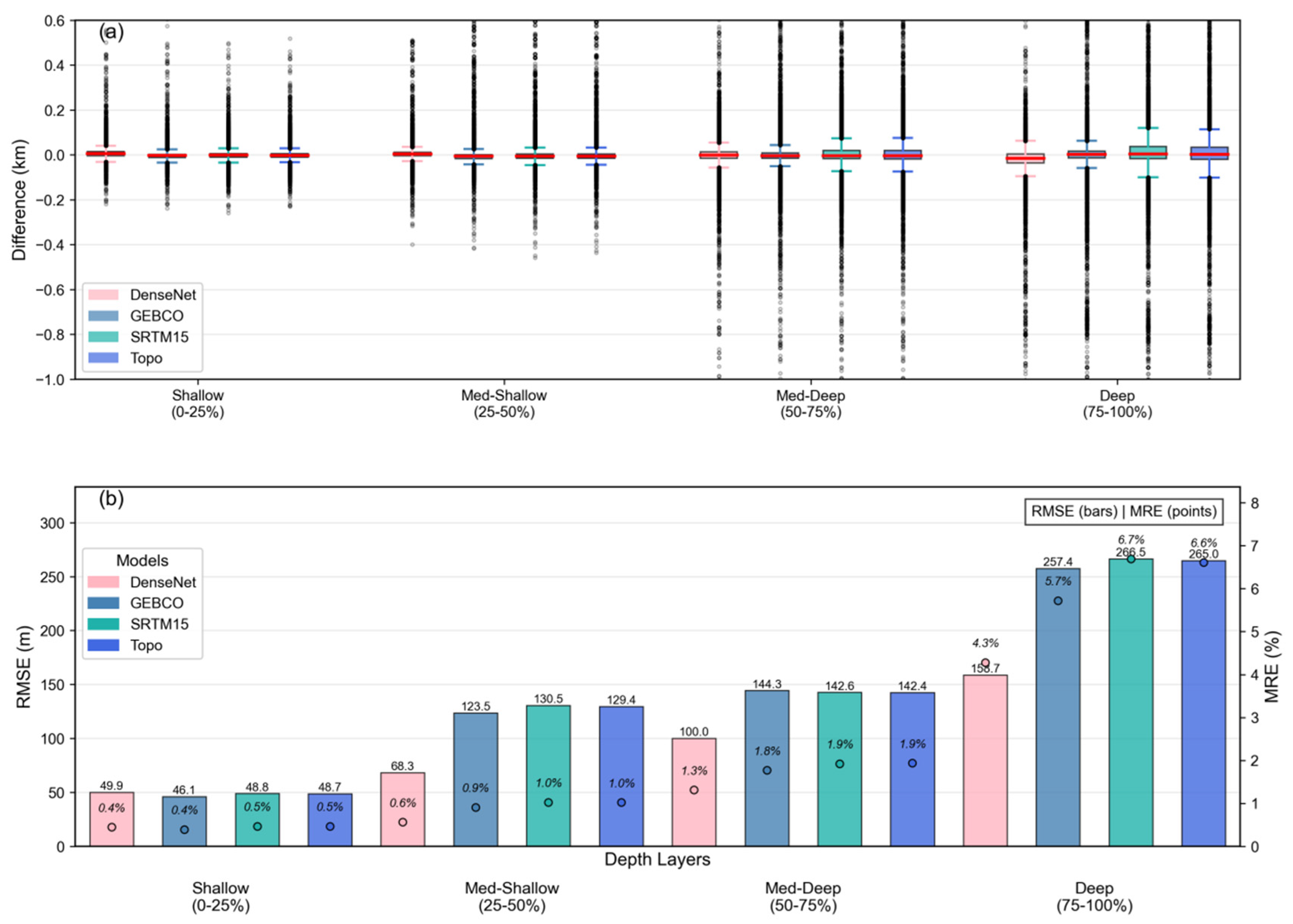
The test set is equally divided into four depth intervals (0–25%, 25–50%, 50–75%, and 75–100%), with each interval containing approximately 10,758 points. As shown in Figure 4, model performance exhibits depth dependence. The DenseNet model’s accuracy advantage is most pronounced in deep-water regions (75–100%), where ship survey data are typically sparse, achieving an RMSE reduction of 44.7% compared to GEBCO_2024. In the shallowest water layer (0–25%), the model’s RMSE is slightly higher than GEBCO_2024 (though still superior to SRTM15+ and Topo_27.1).

3.2. Complex Rift Terrain Modeling Performance

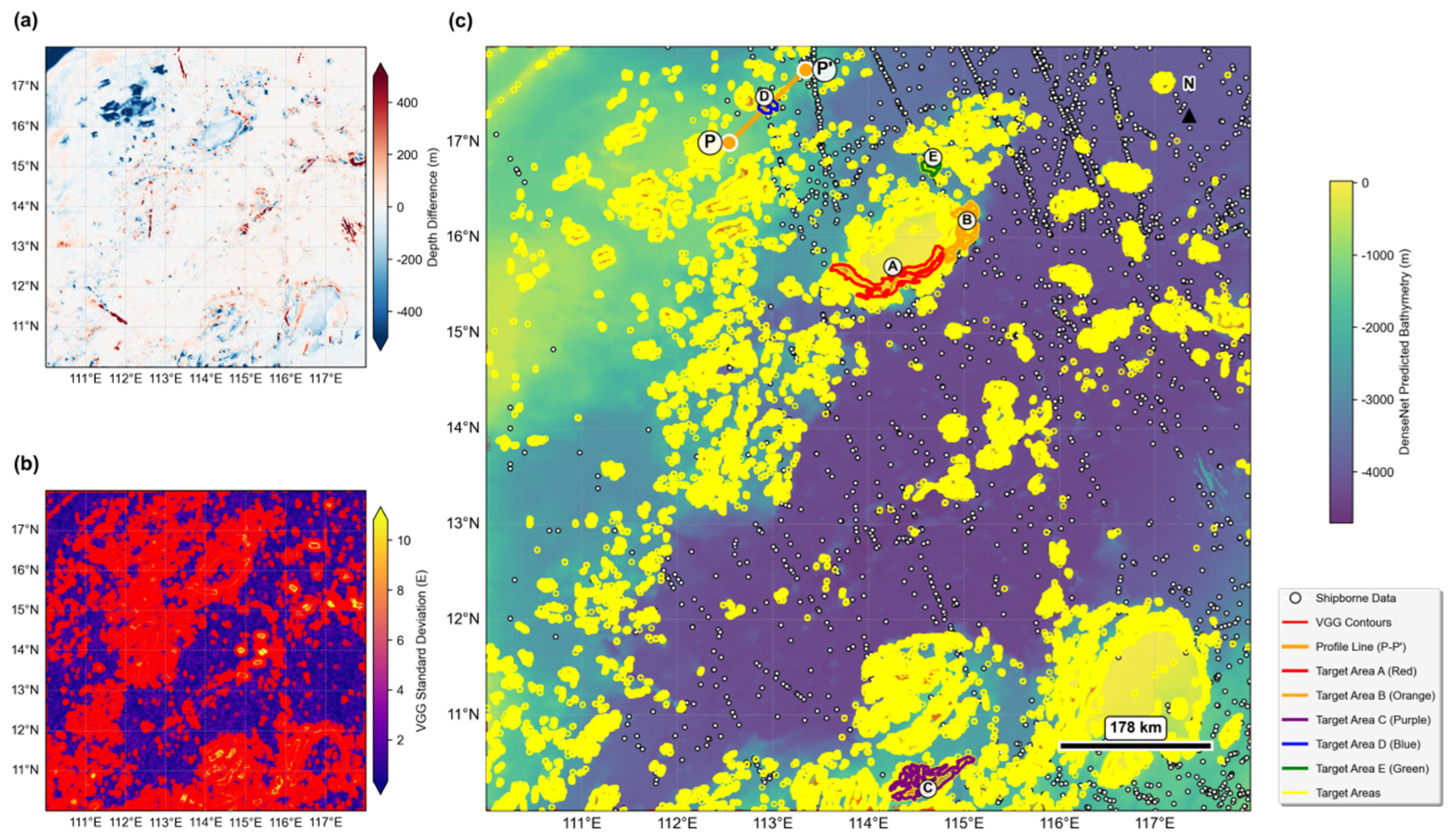
To quantitatively evaluate the model’s performance in extremely complex rift terrains, a dual-threshold identification methodology is developed based on geophysical signatures. The bathymetric difference threshold (|ΔH| > 50 m) captured regions of significant model deviation, while the 80th percentile of vertical gravity gradient variability (σ_VGG > 3.36 E) indicates abrupt topographic transitions. Validation confirmed strong spatial coherence between the thresholds, with 44.0% of high-difference areas concurrently exhibiting high σ_VGG (IoU = 31.3%). Independent shipborne sounding verification shows that 6.6% of control points lay within identified targets, which exhibited RMSE improvements of 69.3–87.1% relative to GEBCO_2024, demonstrating the method’s efficacy in isolating tectonically significant zones with enhanced model performance.

As illustrated in Figure 5, the scientifically identified target areas exhibit significant spatial distribution patterns. The bathymetric difference map (Figure 5a) reveals systematic discrepancies between the DenseNet and GEBCO_2024 models within rift structures, where regions of substantial variation (|ΔH| > 50 m, depicted in red) predominantly cluster at seamount–rift junctions. Figure 5b demonstrates that zones of high vertical gravity gradient variability (σ_VGG, shown in yellow) exhibit strong spatial correspondence with significant depth-difference areas, validating the diagnostic capability of gravity gradient variations for detecting abrupt morphological transitions. Figure 5c presents the final target areas overlaid on the DenseNet-predicted bathymetric background, where yellow-filled polygons denote targets satisfying the dual-threshold criteria, and pentagram markers (A–E) indicate the centroids of the top five quality-ranked targets.

Quantitative evaluation results (

Table 2. Model prediction accuracy comparison for representative submarine rift targets.

Rank	Target	Centroid Coordinates	Area (km2)	Validation Points	DenseNet RMSE (m)	GEBCO_2024 RMSE (m)	Improvement (%)
1	A	114.242°E, 15.596°N	1710	471	64.6	229.1	71.8
2	B	114.992°E, 16.087°N	803	480	75.6	283.9	73.4
3	C	114.608°E, 10.329°N	1492	117	71.1	231.7	69.3
4	D	112.942°E, 17.375°N	242	108	62.8	485.2	87.1
5	E	114.654°E, 16.742°N	214	138	73.9	355.2	79.2

Note: Targets ranked by quality score = Improvement% × ln (Area) × ln (Validation Points).

) confirm the exceptional performance of the DenseNet model in the rift target areas. At Target D, the RMSE decreases substantially from 485.16 m (GEBCO_2024) to 62.80 m, representing a relative improvement of 87.1%. Target A (1710 km²), the largest identified area, achieves a 71.8% error reduction, demonstrating the model’s capacity for large-scale complex terrain reconstruction. Spatial distribution analysis further indicates that the majority of targets reside within high σ_VGG zones (>3.36 E), establishing a robust physical linkage between gravity gradient anomalies and tectonic geomorphology.

3.3. Typical Structural Profile Validation

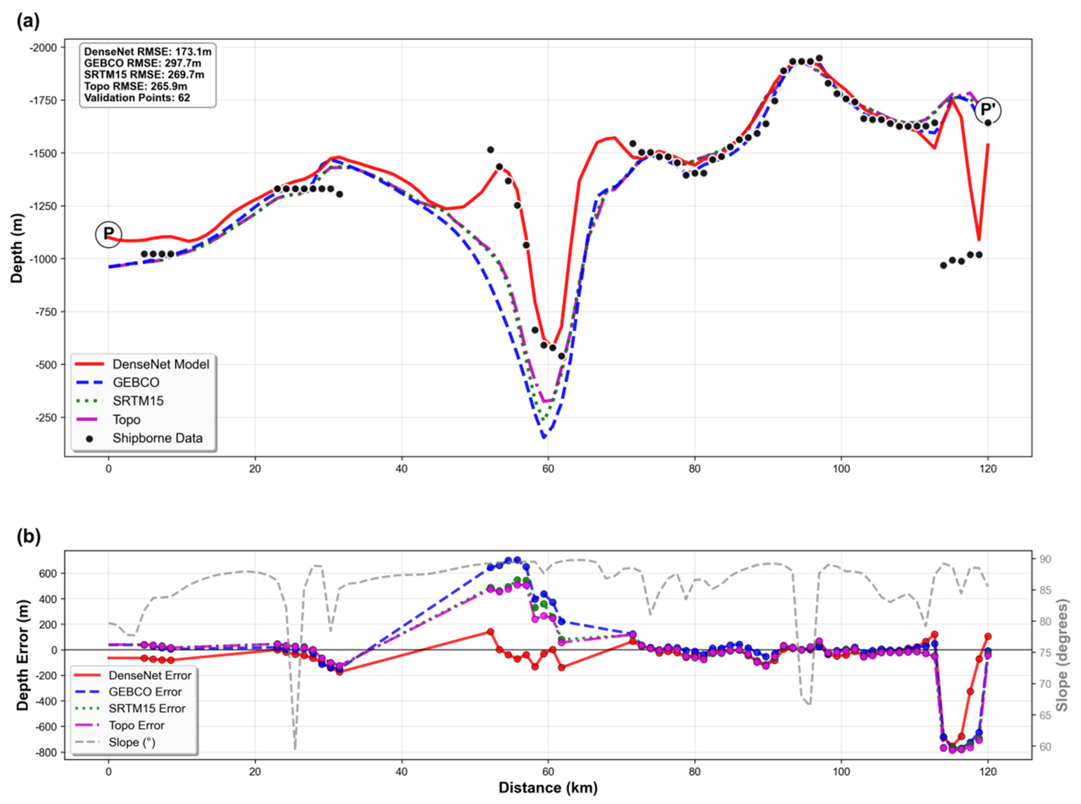
To verify model performance in complex rift terrains, we analyzed bathymetric inversion results along profile PP’ (120 km length) within a region of significant gravity gradient variation (Figure 5c). As shown in Figure 6a, the DenseNet model curve closely aligns with shipborne depths, achieving an RMSE of 173.1 m. It accurately captures abrupt depth changes exceeding 500 m in steep rift slope zones (x = 50–70 km and x = 100–120 km). In contrast, benchmark models exhibit pronounced smoothing effects and systematic biases. Error distribution analysis (Figure 6b) reveals that DenseNet maintains minimal error fluctuations, with deviations stably constrained within ±200 m across the rift section (x = 40–120 km). Benchmark models show significantly amplified errors: GEBCO_2024 reaches 600 m errors in the rift center (x = 50–60 km); SRTM15+ and Topo_27.1 produce error peaks of ∼400 m at abrupt slope transitions (>3° gradient; x = 60 km). Note that DenseNet sustains high prediction accuracy (deviations < 200 m from measurements) even in data-sparse rift core sections, demonstrating its capability to overcome systematic terrain attenuation inherent in conventional models through gravity gradient-constrained inversion.

4. Discussion

4.1. Dominant Role of Vertical Deflection Components in Rift Identification

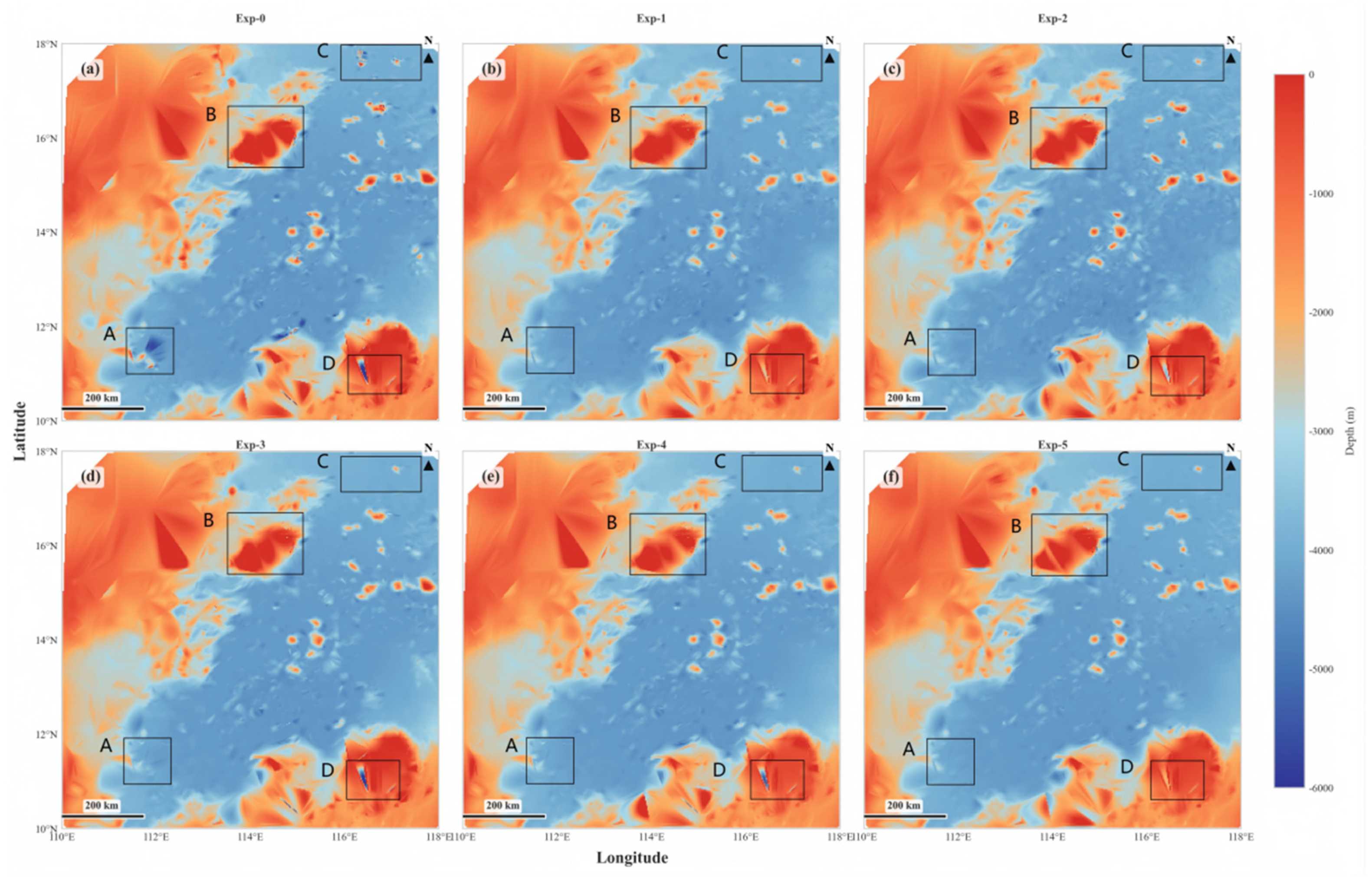
To quantify the contribution of the gravity data, we conduct ablation experiments by sequentially masking different gravity components. Accuracy metrics are computed using the 43,035 test points (

Table 3. Quantitative analysis of the impact of gravity gradient components on accuracy.

Model Configuration	RMSE (m)	R2	ΔRMSE vs. Baseline (m)	Rel. ΔRMSE vs. Baseline (%)
Baseline (GA + VGG + ξ + η + Pos + H_ref)	84.75	0.9935	-	-
Exp-1: GA + Pos + H_ref	178.92	0.9709	+94.17	+111.1%
Exp-2: GA + VGG + Pos + H_ref	175.83	0.9719	+91.08	+107.5%
Exp-3: GA + ξ+η + Pos + H_ref	151.61	0.9791	+66.86	+78.9%
Exp-4: ξ + η + Pos + H_ref	156.62	0.9777	+71.87	+84.8%
Exp-5: No Gravity (Pos + H_ref only)	177.03	0.9715	+92.28	+108.9%

). The experimental results demonstrate that the vertical deflection components (ξ, η) dominate the inversion accuracy for rift structures. Table 3 shows that removing the vertical deflection components (ξ, η) increased the RMSE by 91.08 m (a 107.5% increase relative to the baseline), a significantly larger impact than removing the VGG. Topographic effect comparisons (Figure 7) reveal that the absence of ξ/η causes edge to blur in rift structures (Figure 7d vs. Figure 7a), particularly at seamount–rift junctions (Figure 5c).

This dominance aligns with rift formation mechanics: extensional tectonics generate lateral density contrasts perpendicular to rift axes; during rift formation, extensional tectonics generate lateral density contrasts perpendicular to the extension direction, creating directional gravity gradients [39,40]. The vertical deflection components (ξ = ∂g/∂y, η = ∂g/∂x), as horizontal derivatives of the gravity field, exhibit high sensitivity to near-vertical tectonic boundaries and lateral density discontinuities at crust–mantle interfaces [41]. In contrast, GA primarily integrates mass effects vertically, while the VGG responds strongly to density interfaces with significant vertical extent, limiting its capability to resolve steep rift walls. Visual analysis confirms this, showing edge blurring at seamount–rift junctions when ξ/η are excluded (Figure 7b vs. Figure 7a), while their inclusion reduces the RMSE by 69.3–87.1% in identified rift targets (Table 2).

4.2. Architectural Innovations for Topographic Complexity Adaptation

4.2.1. Adaptive Transition Layer: Resolving the Detail-Efficiency Trade-Off

The dynamic pooling suppression in small feature maps (≤2 × 2) directly addresses steep-slope attenuation in traditional CNNs [42]. Key evidence includes the following: 6.1% RMSE reduction in Q4 steep slopes (

Table 4. Performance comparison between stratified sampling and random sampling models.

Complexity Class	Model	MAE (m)	RMSE (m)	R2	|∆RMSE| (m)
Overall	DenseNet	30.01	84.75	0.9935	6.8464
	Random	40.43	91.59	0.9924
Q1 (Flat)	DenseNet	23.80	81.71	0.9904	5.6911
	Random	32.09	87.40	0.9890
Q2 (Gentle Slope)	DenseNet	26.18	88.41	0.9909	8.8007
	Random	36.01	97.21	0.9890
Q3 (Slope)	DenseNet	26.83	62.88	0.9963	6.4344
	Random	37.63	69.32	0.9955
Q4 (Steep Slope)	DenseNet	43.24	101.39	0.9917	6.6026
	Random	56.00	108.00	0.9906

Note: Q1, Q2, Q3, and Q4 in the table correspond to regions with complexity levels of 0–25%, 25–50%, 50–75%, and 75–100%, respectively, that is, the regions where the complexity ranges from 0.0000 to 0.0233, 0.0233 to 0.0480, 0.0480 to 0.0934, and 0.0934 to 1.0000.

). Accurate capture of 500 m relief jumps in rift margins (Profile PP’, x = 40–60 km, Figure 6a), where benchmark models underestimated depths by >400 m. This innovation preserves high-frequency tectonic features that standard pooling operations discard (e.g., CNN’s 122.53 m RMSE in Table 1).

4.2.2. Curvature Stratification: Mitigating Data Sparsity Bias

Ship soundings are highly uneven (Figure 1b: 145,519 deep vs. 11,466 shallow points), causing conventional models to overfit gentle terrains. Our curvature-based stratification is as follows: reduced steep-slope RMSE by 6.1% (Table 4) by balanced learning. A reduced RMSE for each terrain type confirms the strategy’s effectiveness in enhancing generalization capability within complex regions.

Despite strong performance in deep waters, the model exhibits slightly higher errors than GEBCO_2024 in shallow depths (0–25%). It is also noteworthy that this limitation likely stems from two key factors: first, the sparsity of ship soundings in shallow zones (accounting for only 5.3% of the total data), which reduces the model’s training constraints for shallow terrain; second, the complex gravity–topography coupling in shallow areas, where hydrodynamic noise and non-bathymetric signals (e.g., from marine sediments) further complicate the signal-to-noise ratio. While the data-driven model attempts to prioritize bathymetry-relevant features, the interference from these shallow-specific factors still represents a potential source of uncertainty.

5. Conclusions

We developed an enhanced DenseNet framework integrating multi-gravity-component fusion and curvature-adaptive stratification to address bathymetric inversion challenges in tectonically complex regions. By constructing a 16 × 16 × 9 input tensor from shipborne soundings, gravity derivatives (GA, VGG, ξ, η), and GEBCO_2024, the model achieved a global RMSE of 84.75 m—47.6% lower than GEBCO_2024. Crucially, vertical deflection components (ξ/η) were identified as the dominant physical constraint for rift recognition, with their removal increasing prediction errors by 107.5% (significantly exceeding impacts from other gravity components). Architectural innovations—notably the adaptive transition layer that suppresses pooling on small feature maps—reduced steep-slope RMSE by 6.1%, outperforming standard CNNs. Concurrently, curvature-based stratification mitigated ship-data sparsity bias, enhancing prediction stability by 6.1% across complex geomorphologies.

Furthermore, future research will extend this framework to mid-ocean ridge regions and incorporate physical constraints into data-driven models—specifically by exploring the integration of external models of sediment thickness (e.g., from global sediment databases or seismic surveys) and crustal structure to preprocess gravity inputs. This strategy aims to more explicitly isolate the gravitational signature of bedrock topography, which could not only further enhance inversion accuracy in regions with thick sediment cover but also address the current limitation of slightly higher errors in shallow water areas, ultimately supporting the establishment of high-precision seafloor topographic models in global environments.

References

1. An, D.; Guo, J.; Li, Z.; Ji, B.; Liu, X.; Chang, X. Improved Gravity-Geologic Method Reliably Removing the Long-Wavelength Gravity Effect of Regional Seafloor Topography: A Case of Bathymetric Prediction in the South China Sea. IEEE Trans. Geosci. Remote Sens. 2022, 60, 4211912. [Google Scholar] [CrossRef]
2. Zhou, S.; Guo, J.; Zhang, H.; Jia, Y.; Sun, H.; Liu, X.; An, D. SDUST2023BCO: A Global Seafloor Model Determined from a Multi-Layer Perceptron Neural Network Using Multi-Source Differential Marine Geodetic Data. Earth Syst. Sci. Data 2025, 17, 165–179. [Google Scholar] [CrossRef]
3. Abulaitijiang, A.; Andersen, O.B.; Sandwell, D. Improved Arctic Ocean Bathymetry Derived DTU17 Gravity Model. Earth Space Sci. 2019, 6, 1336–1347. [Google Scholar] [CrossRef]
4. Baudry, N.; Calmant, S. Seafloor Mapping from High-Density Satellite Altimetry. Mar. Geophys. Res. 1996, 18, 135–146. [Google Scholar] [CrossRef]
5. Fan, D.; Li, S.; Feng, J.; Sun, Y.; Xu, Z.; Huang, Z. A New Global Bathymetry Model STO_IEU2020. Remote Sens. 2022, 14, 5744. [Google Scholar] [CrossRef]
6. Hu, M.; Jin, T.; Jiang, W.; Chu, Y.; Wen, H.; Li, J. Bathymetry Model in the Northwestern Pacific Ocean Predicted from Satellite Altimetric Vertical Gravity Gradient Anomalies and Ship-Board Depths. Mar. Geod. 2022, 45, 24–46. [Google Scholar] [CrossRef]
7. Sandwell, D.T.; Goff, J.A.; Gevorgian, J.; Harper, H.; Kim, S.-S.; Yu, Y.; Tozer, B.; Wessel, P.; Smith, W.H.F. Improved Bathymetric Prediction Using Geological Information: SYNBATH. Earth Space Sci. 2022, 9, e2021EA002069. [Google Scholar] [CrossRef]
8. Harper, H.; Sandwell, D.T. Global Predicted Bathymetry Using Neural Networks. Earth Space Sci. 2024, 11, e2023EA003199. [Google Scholar] [CrossRef]
9. Hsiao, Y.-S.; Kim, J.; Kim, K.B.; Lee, B.; Hwang, C. Bathymetry Estimation Using the Gravity-Geologic Method: An Investigation of Density Contrast Predicted by the Downward Continuation Method. Terr. Atmos. Ocean. Sci. 2011, 22, 347–358. [Google Scholar] [CrossRef]
10. Kim, J.W.; von Frese, R.R.B.; Lee, B.Y.; Roman, D.R.; Doh, S.-J. Altimetry-Derived Gravity Predictions of Bathymetry by the Gravity-Geologic Method. Pure Appl. Geophys. 2011, 168, 815–826. [Google Scholar] [CrossRef]
11. Kim, K.B.; Lee, C.K. Bathymetry Change Investigation of the 2011 Tohoku Earthquake. J. Korean Soc. Surv. Geod. Photogramm. Cartogr. 2015, 33, 181–192. [Google Scholar] [CrossRef]
12. Kim, K.B.; Yun, H.S. Satellite-Derived Bathymetry Prediction in Shallow Waters Using the Gravity-Geologic Method: A Case Study in the West Sea of Korea. KSCE J. Civ. Eng. 2018, 22, 2560–2568. [Google Scholar] [CrossRef]
13. Hsiao, Y.-S.; Hwang, C.; Cheng, Y.-S.; Chen, L.-C.; Hsu, H.-J.; Tsai, J.-H.; Liu, C.-L.; Wang, C.-C.; Liu, Y.-C.; Kao, Y.-C. High-Resolution Depth and Coastline over Major Atolls of South China Sea from Satellite Altimetry and Imagery. Remote Sens. Environ. 2016, 176, 69–83. [Google Scholar] [CrossRef]
14. Wei, Z.; Guo, J.; Zhu, C.; Yuan, J.; Chang, X.; Ji, B. Evaluating Accuracy of HY-2A/GM-Derived Gravity Data with the Gravity-Geologic Method to Predict Bathymetry. Front. Earth Sci. 2021, 9, 636246. [Google Scholar] [CrossRef]
15. Dixon, T.H.; Parke, M.E. Bathymetry Estimates in the Southern Oceans from Seasat Altimetry. Nature 1983, 304, 406–411. [Google Scholar] [CrossRef]
16. Baudry, N.; Calmant, S. 3-D Modelling of Seamount Topography from Satellite Altimetry. Geophys. Res. Lett. 1991, 18, 1143–1146. [Google Scholar] [CrossRef]
17. Smith, W.H.F.; Sandwell, D.T. Bathymetric Prediction from Dense Satellite Altimetry and Sparse Shipboard Bathymetry. J. Geophys. Res. Solid Earth 1994, 99, 21803–21824. [Google Scholar] [CrossRef]
18. Calmant, S.; Berge-Nguyen, M.; Cazenave, A. Global Seafloor Topography from a Least-Squares Inversion of Altimetry-Based High-Resolution Mean Sea Surface and Shipboard Soundings. Geophys. J. Int. 2002, 151, 795–808. [Google Scholar] [CrossRef]
19. Ramillien, G.; Wright, I.C. Predicted Seafloor Topography of the New Zealand Region: A Nonlinear Least Squares Inversion of Satellite Altimetry Data. J. Geophys. Res. Solid Earth 2000, 105, 16577–16590. [Google Scholar] [CrossRef]
20. Sun, H.; Jin, T.; Feng, Y.; Sun, W.; Zhou, M.; Sun, H. The Nonlinear Effects in Bathymetric Prediction from Altimetric Gravity Data. J. Geod. 2025, 99, 39. [Google Scholar] [CrossRef]
21. Xu, H.; Yu, J. Using an Iterative Algorithm to Predict Topography From Vertical Gravity Gradients and Ship Soundings. Earth Space Sci. 2022, 9, e2022EA002437. [Google Scholar] [CrossRef]
22. Fan, D.; Li, S.; Li, X.; Yang, J.; Wan, X. Seafloor Topography Estimation from Gravity Anomaly and Vertical Gravity Gradient Using Nonlinear Iterative Least Square Method. Remote Sens. 2021, 13, 64. [Google Scholar] [CrossRef]
23. Yang, J.; Jekeli, C.; Liu, L. Seafloor Topography Estimation From Gravity Gradients Using Simulated Annealing. J. Geophys. Res. Solid Earth 2018, 123, 6958–6975. [Google Scholar] [CrossRef]
24. Xu, C.; Li, J.; Jian, G.; Wu, Y.; Zhang, Y. An Adaptive Nonlinear Iterative Method for Predicting Seafloor Topography From Altimetry-Derived Gravity Data. J. Geophys. Res. Solid Earth 2023, 128, e2022JB025692. [Google Scholar] [CrossRef]
25. Jiang, X.; Guo, J.; Lin, M.; Sun, H.; Jiang, T. Enhanced Gravity-Geologic Method to Predict Bathymetry by Considering Non-Linear Effects of Surrounding Seafloor Topography. Geophys. J. Int. 2024, 239, 754–767. [Google Scholar] [CrossRef]
26. Sun, H.; Feng, Y.; Fu, Y.; Sun, W.; Peng, C.; Zhou, X.; Zhou, D. Bathymetric Prediction Using Multisource Gravity Data Derived From a Parallel Linked BP Neural Network. J. Geophys. Res. Solid Earth 2022, 127, e2022JB024428. [Google Scholar] [CrossRef]
27. An, D.; Feng, W.; Chen, X.; Sun, M.; Zhang, Z.; Meng, Y.; Zhong, M. Predicting Intermediate Wavelength Depth Using a Deep Neural Network Combined with Gravity Data in the Sea of Japan. Int. J. Digit. Earth 2024, 17, 2430679. [Google Scholar] [CrossRef]
28. Annan, R.F.; Wan, X. Recovering Bathymetry of the Gulf of Guinea Using Altimetry-Derived Gravity Field Products Combined via Convolutional Neural Network. Surv. Geophys. 2022, 43, 1541–1561. [Google Scholar] [CrossRef]
29. Zhou, S.; Liu, X.; Sun, Y.; Chang, X.; Jia, Y.; Guo, J.; Sun, H. Predicting Bathymetry Using Multisource Differential Marine Geodetic Data with Multilayer Perceptron Neural Network. Int. J. Digit. Earth 2024, 17, 2393255. [Google Scholar] [CrossRef]
30. Zhou, S.; Liu, X.; Guo, J.; Jin, X.; Lei, Y.; Sun, Y.; Sun, H. Bathymetry of the Gulf of Mexico Predicted with Multilayer Perceptron From Multisource Marine Geodetic Data. IEEE Trans. Geosci. Remote Sens. 2023, 61, 4208911. [Google Scholar] [CrossRef]
31. Trung, N.N.; Lee, S.-M.; Que, B.C. Satellite Gravity Anomalies and Their Correlation with the Major Tectonic Features in the South China Sea. Gondwana Res. 2004, 7, 407–424. [Google Scholar] [CrossRef]
32. Yan, Q.; Shi, X.; Yuan, L.; Yan, S.; Liu, Z. Tectono-Magmatic Evolution of the Philippine Sea Plate: A Review. Geosyst. Geoenviron. 2022, 1, 100018. [Google Scholar] [CrossRef]
33. GEBCO. Gridded Bathymetry Data. Available online: https://www.gebco.net/data-products/gridded-bathymetry-data (accessed on 27 July 2025).
34. Tozer, B.; Sandwell, D.T.; Smith, W.H.F.; Olson, C.; Beale, J.R.; Wessel, P. Global Bathymetry and Topography at 15 Arc Sec: SRTM15+. Earth Space Sci. 2019, 6, 1847–1864. [Google Scholar] [CrossRef]
35. Marks, K.M.; Smith, W.H.F. Radially Symmetric Coherence between Satellite Gravity and Multibeam Bathymetry Grids. Mar. Geophys. Res. 2012, 33, 223–227. [Google Scholar] [CrossRef]
36. Wang, D.; Dong, J.; Tang, L.; Ma, M.; Xie, T. An Automatic Generalization Method of a Block-Based Digital Depth Model Based on Surface Curvature Features. J. Mar. Sci. Eng. 2024, 12, 2299. [Google Scholar] [CrossRef]
37. Huang, G.; Liu, Z.; Van Der Maaten, L.; Weinberger, K.Q. Densely Connected Convolutional Networks. In Proceedings of the 2017 IEEE Conference on Computer Vision and Pattern Recognition (CVPR), Honolulu, HI, USA, 21–26 July 2017; pp. 2261–2269. [Google Scholar]
38. Zhu, Y.; Newsam, S. DenseNet for Dense Flow. In Proceedings of the 2017 IEEE International Conference on Image Processing (ICIP), Beijing, China, 17–20 September 2017; pp. 790–794. [Google Scholar]
39. Ekinci, Y.L. A Comparative Study on Computing Horizontal Derivatives of Gravity Data for Geological Contact Mapping. Geol. Bull. Turk. 2017, 60, 209–221. [Google Scholar] [CrossRef]
40. Kim, S.-S.; Wessel, P. New Analytic Solutions for Modeling Vertical Gravity Gradient Anomalies. Geochem. Geophys. Geosyst. 2016, 17, 1915–1924. [Google Scholar] [CrossRef]
41. Prasad, K.N.D.; Nguyen, D.V.; Le-Huy, M.; Tran, K.V.; Do, T.D.; Pham, L.T.; Rehman, H. Mapping Structural Geometry and Tectonics of the Central Continental Margin of Vietnam and Adjacent Areas Using an Enhanced Horizontal Gradient of Gravity Data. Tectonophysics 2025, 905, 230719. [Google Scholar] [CrossRef]
42. Krizhevsky, A.; Sutskever, I.; Hinton, G.E. ImageNet Classification with Deep Convolutional Neural Networks. In Proceedings of the Advances in Neural Information Processing Systems, Lake Tahoe, NV, USA, 3–6 December 2012; Volume 25. [Google Scholar]
Figure 1. Regional overview and study area. (a) Regional bathymetric map of the Northwest Pacific based on GEBCO_2024. The red rectangle delineates the study area (110°E–118°E, 10°N–18°N). Major geographic features are annotated. (b) High-resolution bathymetry of the study area showing complex seafloor morphology. Three bathymetric point datasets are displayed: yellow points: 11,466 shallow measurements (<1000 m); orange points: 65,925 mid-depth measurements (1000–3000 m); red points: 145,519 deep measurements (>3000 m).
Remotesensing 17 03453 g001
Figure 2. Feature tensor construction and training model framework. (a) Data preprocessing workflow, showing the pipeline from raw bathymetry data cleaning through 3σ criterion and curvature-based stratified sampling to multi-source feature integration. Gravity components (GA, VGG, ξ, η) and reference depth are standardized via RobustScaler, while spherical coordinate encodings are incorporated directly. (b) Improved DenseNet architecture comprising dense blocks with adaptive transition layers that suppress pooling on small feature maps to preserve high-frequency tectonic features, followed by a depth regression module with fully connected layers. The legend illustrates the dense connectivity and adaptive transition mechanisms.
Remotesensing 17 03453 g002
Figure 3. Three-dimensional topographic rendering of the seamounts group region in the central South China Sea retrieved by the improved DenseNet model.
Remotesensing 17 03453 g003
Figure 4. RMSE comparison of different models (DenseNet, GEBCO_2024, SRTM15+, and Topo_27.1) across four equal-depth intervals (0–25%, 25–50%, 50–75%, and 75–100%). (a) Presents each model’s relative error distribution trend and error fluctuation characteristics across shallow (0–25%), medium-shallow (25–50%), medium-deep (50–75%), and deep (75–100%) water intervals. (b) Uses combined bar charts (for RMSE) and scatter plots (for MRE) to compare each model’s performance in the above depth intervals based on the two accuracy metrics.
Remotesensing 17 03453 g004
Figure 5. Rift target identification and model improvement validation based on gravity gradient features. (a) Inter-model depth differences between DenseNet and GEBCO_2024 (red: |ΔH| > 50 m). (b) VGG variation intensity (yellow: σ_VGG > 3.36 E). (c) Target distribution over DenseNet bathymetry (A–E: Top 5 targets in Table 2).
Remotesensing 17 03453 g005
Figure 6. Bathymetric profile along line PP’ (~120 km) shown in Figure 5c. (a) Comparison of bathymetric profile characteristics. (b) Comparison of the coupling relationship between error distribution and terrain slope.
Remotesensing 17 03453 g006
Figure 7. Topographic effect comparison of ablation experiments (focusing on a typical rift area). (a) Baseline model (complete gravity: GA + VGG + ξ+η + Position + H_ref). (b) Exp-1 (GA + Position + H_ref only). (c) Exp-2 (GA + VGG + Position + H_ref). (d) Exp-3 (GA + ξ+η + Position + H_ref). (e) Exp-4 (ξ + η+Position + H_ref). (f) Exp-5 (No gravity, Position + H_ref only). The black rectangles (labeled A–D) highlight representative areas where the exclusion of specific gravity components, particularly the vertical deflection components (ξ, η), leads to significant topographic degradation, such as blurred rift edges and diminished seamount-rift junction definition. Color shading represents depth.
Remotesensing 17 03453 g007