Highlights
What are the main findings?
- A distance-transform-based spatiotemporal model, combining Laplacian inpainting and B-Spline fitting with a Bézier decay function which offers significant improvements in NDVI approximation accuracy over other methods that work within similar computational budget, across 16 Canadian fields (2018–2023).
- The model is computationally efficient, processing in seconds on consumer level hardware using single-source data, and empirically optimized decay parameters enhance performance in diverse cloud patterns.
What is the implication of the main finding?
- It provides a computationally efficient and interpretable solution for cloud-contaminated satellite imagery, enabling reliable vegetation monitoring without dependency on multiple data sources.
- Improves applications like peak green day identification that are used in agriculture management systems.
Abstract
One widely used method for analyzing vegetation growth from satellite imagery is the Normalized Difference Vegetation Index (NDVI), a key metric for assessing vegetation dynamics. NDVI varies not only spatially but also temporally, which is essential for analyzing vegetation health and growth patterns over time. High-resolution, cloud-free satellite images, particularly from publicly available sources like Sentinel, are ideal for this analysis. However, such images are not always available due to cloud and shadow contamination. To address this limitation, we propose a model that integrates both the temporal and spatial aspects of the data to approximate the missing or contaminated regions. In this method, we separately approximate NDVI using spatial and temporal components of the time-varying satellite data. Spatial approximation near the boundary of the missing data is expected to be more accurate, while temporal approximation becomes more reliable for regions further from the boundary. Therefore, we propose a model that leverages the distance transform to combine these two methods into a single, weighted model, which is more accurate than either method alone. We introduce a new decay function to control this transition. We evaluate our spatiotemporal model for approximating NDVI across 16 farm fields in Western Canada from 2018 to 2023. We empirically determined the best parameters for the decay function and distance-transform-based model. The results show a significant improvement compared to using only spatial or temporal approximations alone (up to a 263% improvement as measured by RMSE relative to the baseline). Furthermore, our model demonstrates a notable improvement compared to simple combination (up to 51% improvement as measured by RMSE) and Spatiotemporal Kriging (up to 28% improvement as measured by RMSE). Finally, we apply our spatiotemporal model in a case study related to improving the specification of the peak green day for numerous fields.
1. Introduction
Monitoring and analyzing vegetation are essential for understanding ecosystem dynamics and improving agricultural productivity. Tracking temporal changes in vegetation is crucial for understanding ecological trends, while monitoring crop growth, development, and condition is vital for enhancing crop management and optimizing yields [1]. Optical satellite imagery is a powerful tool for global vegetation and crop monitoring. Publicly available Earth observation satellites like Sentinel-2, the Landsat series, and MODIS provide essential optical imagery for vegetation monitoring. A key metric extracted from satellite imagery is the Normalized Difference Vegetation Index (NDVI), which quantifies vegetation health [2]. NDVI is a widely used and effective indicator for monitoring crop conditions and detecting environmental changes over time [1,3].
Using time-varying satellite data, the calculation of NDVI is straightforward and can be determined by combining multiple bands of satellite images. However, publicly available satellite imagery is produced every 3 to 16 days, depending on the satellite and the location on Earth, and is susceptible to obstructions such as clouds and cloud shadows. This can result in situations where NDVI cannot be calculated for crop monitoring for extended periods, affecting NDVI analyses, while also highlighting the broader challenge of extracting reliable vegetation metrics from large-scale geospatial datasets—a key concern in big geospatial data and advanced satellite-based modelling.
Current methods either rely on combining multiple sensors from multiple satellites using complex computations [4,5,6,7,8,9] or approximate the missing NDVI using simple mathematical forms, which fail to accurately approximate the missing NDVI [10,11]. To address the challenge of missing data and data contamination in resource-constrained environments, we introduce a model that combines spatial and temporal approximation methods. For spatial approximation, we employ an inpainting technique based on Partial Differential Equations (PDE) to approximate the missing areas in each image [12,13]. For the temporal aspect, we utilize B-Spline fitting, a simple yet effective method for approximating time-series data with smooth curves [14,15]. B-Splines provide a flexible approach for approximating the missing parts of a time series, even if it exhibits complex patterns, such as those seen in NDVI due to climate and human activity [16,17].
Combining spatial and temporal approximation may not necessarily lead to better accuracy. The approximation error of the spatial method is related to the homogeneity and size of the missing area. Meanwhile, the accuracy of the temporal method depends primarily on the temporal resolution of the data available to the model. Consequently, the spatial approximation tends to be more effective nearer to the perimeter of the missing area, whereas the temporal method is more effective farther from the perimeter.
A simple combination method that does not consider these properties may result in lower approximation accuracy; one may achieve the best or worst of both methods. The main hypothesis of this work is that the impact of the spatial approximation must be controlled by the distance of the missing pixel from the perimeter of the missing area. This requires a weight function to control this impact. By incorporating this mechanism into a unified spatial–temporal model, we hypothesize that the resulting weighted approach will enhance overall reconstruction accuracy. To implement the weighting mechanism, we propose a weighted combination based on the distance from the perimeter, utilizing the distance transform (DT). The distance transform generates a distance map, where the value of each pixel represents its distance from the nearest perimeter of an object within the image [18]. Our weight function is defined by applying a decay function to the result of a distance transform to control the transition between spatial and temporal approximations. To have full control over the weight function, we introduce a parametric decay function using Bézier curves. We empirically evaluate and derive the decay function parameters through a dataset that includes the missing patterns in our data.
To evaluate our final model’s performance, we compare the results against known ground truth using obstruction-free NDVI images. We then systematically introduce obstruction masks to synthesize regions and compare the model’s output for these synthesized regions to the ground-truth images. The accuracy of the approximation is quantified using Root Mean Square Error (RMSE). For a fair comparison, we use a dataset of real-world cloud and shadow patterns from 16 farm fields in western Canada, sourced from the Sentinel-2 platform between 2018 and 2023. These patterns are used as obstruction masks and to derive the decay function parameters. The results show a significant improvement compared to using only purely spatial, purely temporal approximations and the simple weighted combined spatiotemporal model, as measured by RMSE. As a case study, we identify the peak green day for fields using Sentinel-2 imagery during the growth season. The NDVI on this day serves as a performance indicator for the fields. This peak green data is used for various applications, such as creating zone delineation maps for field management [19,20].
The main contribution of this work is the development of a novel distance-transform-based spatiotemporal model for NDVI reconstruction, designed to approximate missing data both accurately and efficiently. The model leverages a distance transform alongside a decay function to regulate transitions between spatial and temporal approximations. Unlike machine learning approaches, which often require rich datasets, significant computational resources, and extensive training, the proposed method creates reliable results using only single-source NDVI data, with processing times measured in seconds. This makes our model a computationally lightweight and scalable alternative, particularly suited to data-constrained environments. Furthermore, its strength lies not in isolated spatial or temporal techniques but in its ability to seamlessly integrate both components into a unified, adaptive framework. Additionally, the model provides tunable flexibility through well-known interactive curve models—specifically, B-Spline and Bézier curve parameters—allowing domain experts to refine reconstruction outputs in human-in-the-loop workflows.
To enhance the depth and structure of our literature review, we have elected to present the related work in a separate section rather than within the Introduction. This approach enables a more thorough analysis of a wider spectrum of pertinent studies, thereby improving both the clarity and overall organization of the paper.
2. Related Work
To contextualize this work, we start by showing the importance of NDVI (Section 2.1) and time-varying satellite imaging (Section 2.2). Then we cover spatial approximation methods (Section 2.3), temporal methods (Section 2.4) and Spatiotemporal models (Section 2.5) used for approximating missing parts of time-varying NDVI data. Lastly, we explore the machine learning methods for approximating NDVI data (Section 2.6).
2.1. NDVI
Spectral vegetation indices are vital tools in remote sensing for assessing vegetation health by analyzing the reflectance of different wavelengths of light [21]. These indices, derived from satellite or aerial imagery, help in monitoring plant health, growth, and stress by combining information from multiple spectral bands. Among them, the Normalized Difference Vegetation Index (NDVI) is particularly significant due to its simplicity and effectiveness [22]. This index provides a clear, standard metric of vegetation health, making it a widely used and reliable indicator in environmental monitoring and agricultural management [23]. In agriculture, NDVI aids in evaluating crop conditions, forecasting yields, and optimizing resource management practices like irrigation and fertilization, thereby enhancing precision farming techniques [1,24]. Environmental applications of NDVI include tracking deforestation, assessing land degradation, and studying the impacts of climate change on vegetation dynamics, which are crucial for biodiversity conservation and ecological research [25,26,27].
A useful vegetation performance metric derived from NDVI imagery is the peak green image, which captures the maximum NDVI values observed over a specified time period and serves as an indicator of optimal vegetation conditions in agricultural fields [19,20]. The concept of the peak green day refers to the specific date whose NDVI image most closely reflects ideal vegetation conditions—defined by the pixelwise maximum NDVI across the field (referred to as the ideal image). Since individual pixels reach their peak NDVI on different dates, the ideal image may not correspond to any single acquisition date. However, the peak green day image is selected from the available daily images as the one that best approximates these optimal conditions across the entire field.
2.2. Time-Varying Satellite Imaging and Its Applications
Time-varying satellite imaging (TVSI) refers to sequential satellite images of the same area over a period of time. In literature, TVSI is also denoted as “Satellite Image Time Series” (SITS) [28]. TVSI has become an essential tool for observing and understanding dynamic Earth processes, as it captures both the temporal and spatial dimensions of the satellite images [29,30]. TVSI is well-suited for applications that need to detect or analyze the changes to an area over time, such as drought monitoring, fire impact assessment and crop yield estimation [31,32,33]. As NDVI can be used for large-scale analysis of an area, it is common to calculate the NDVI of each pixel in all the images in TVSI, creating the “NDVI-TVSI” as the result [34]. NDVI-TVSI is especially important in precision agriculture, as it is a vital part of many analysis methods that produce results similar to more costly and labour-intensive methods of monitoring the agricultural field [35]. As such, NDVI-TVSI is used in a plethora of methods in precision agriculture [19,20,36].
2.3. Image Inpainting
Image inpainting is the process of reconstructing lost or deteriorated parts of an image by mathematically propagating information from the surrounding areas [13]. Techniques like Laplacian inpainting solve the Laplace equation to smoothly interpolate pixel values, ensuring that the transition between known and unknown regions is gradual and visually seamless [37]. Poisson inpainting extends this approach by solving the Poisson equation, which takes into account the gradient of the image to preserve edge information and texture continuity. This method also minimizes the difference between the gradients of the inpainted area and its surroundings, effectively blending the new content with the existing image [38].
To approximate the obstructed part of a TVSI for NDVI analysis, image inpainting could be employed. In image inpainting, the values of missing parts of the image are approximated based on the available values in the neighbouring regions. A sparse dictionary learning method has been proposed, which uses the pattern of other NDVI images to create a dictionary of patterns (a sparse set of representative image patches learned from the data) and then uses this information to fill the missing part of the NDVI image by matching the patterns based on the non-missing pixels [39]. There are also methods that use partial differential equations (PDE) to use the smoothness of transition between neighbouring pixels in the NDVI image to propagate the values from the known pixels to unknown pixels smoothly. The Navier–Stokes-Based method proposed in [40] does exactly that. Similarly, the Laplacian method we employ in this work also falls into the PDE group of methods.
Image inpainting methods are important in approximating missing parts of NDVI-TVSI, but they only use one aspect of NDVI-TVSI which is the neighbouring regions. To better approximate the missing data, we should also use the temporal aspect of NDVI-TVSI, as it has information that could be useful in better approximating the missing regions.
2.4. Temporal Approximation
Temporal methods are a natural fit for approximating the missing parts of an NDVI image, as each pixel in a TVSI can be viewed as a time series that can be approximated using various available time series approximation methods. A linear regression model, in conjunction with a Savitzky-Golay filter, has been employed to approximate NDVI values [41]. Wavelet transform has also been used to smooth out and approximate missing NDVI values to research vegetation dynamics [42]. Harmonic analysis has also been used to approximate missing NDVI values in MODIS satellite images [43]. Approximating NDVI by fitting a piecewise linear curve, an asymmetric Gaussian curve, a double logistic curve, a polynomial curve, and a uniform cubic spline curve has also been proposed, with the uniform cubic spline having the all-around best solution for approximating NDVI values using temporal data [44]. Although there is no precedence for using B-Spline for approximating NDVI-TVSI in the literature, B-Spline has been used for fitting a spline to a time series, due to the numerical stability and local control [45,46]. A double-logistic model has also been used to find a prediction over NDVI historical data [2]. The use of the Fourier series to approximate NDVI is also explored in this context [44].
Similar to spatial methods, temporal methods only use one aspect of NDVI-TVSI, which is the temporal aspect, and ignore the spatial aspect. This means that there is room for improving the approximation of missing parts of NDVI-TVSI using both the spatial and temporal aspects of NDVI-TVSI. On top of that, in methods that only use the temporal aspect of NDVI-TVSI in the literature, none of them use B-Spline. The most similar method used is the cubic spline. B-Spline has local control, better numerical stability and better computational efficiency [47]. This results in B-Spline producing better approximations in comparison to cubic splines when used properly [48].
2.5. Spatiotemporal
In the literature, the term Spatiotemporal refers to two distinct ideas that we need to distinguish from each other. Sometimes, the term Spatiotemporal refers to the combination of two satellite image sources, one with high temporal resolution but low pixel resolution, the other with high pixel resolution but low temporal resolution [49]. We call this “data fusion” in this work. In other times, Spatiotemporal refers to using both the temporal and spatial aspects of a TVSI, as each pixel in a TVSI has both nearby pixels in the image it is on and also has the value of that same pixel position in other images in the time series [50]. In this work, we are interested in the latter definition of Spatiotemporal and only use this term in the context of using both the temporal and spatial aspects of a TVSI.
Some data fusion works combine multiple satellite images from different sources [49] or use different datasets such as climate data [51] to create an improved historical NDVI dataset. They do not approximate NDVI directly, but by improving the temporal and spatial resolution of the NDVI dataset available, they add NDVI values to some days and areas that did not have a valid NDVI value before.
Outside of data fusion, methods that use the spatial and temporal dimensions of NDVI-TVSI usually rely on machine learning techniques to combine these two aspects. One work that does not rely on machine learning is [36]. In this work, Amirfakhrian et al. propose the “Variational-Based Spatial–Temporal” method, which is an image blending method to combine a temporal approximation in the form of an asymmetric double-sigmoid curve fitting and a spatial approximation in the form of a Laplacian approximation of missing areas.
Combining the spatial and temporal aspects of NDVI-TVSI in approximating NDVI can be done in one of two ways. Either the spatial and temporal aspects are used by two separate methods, each coming up with separate results, which are then combined after the fact. Or the spatial and temporal aspects are both used in the process of producing the approximation. In the first approach, current methods can be improved by using the fact that spatial solutions have better approximation performance in the parts of the missing area that are closer to the perimeter of the missing area. The methods that take the second approach are all data fusion methods, which usually use data from 3 or more different sensors. This means that they need to solve many problems, such as how different data from different sensors relate to each other and how to combine information with different resolutions [49]. This means that these methods use several times more data, computing power and computation time to produce results comparable to those of our method.
Spatiotemporal fusion methods include linear approaches like STARFM (Spatial and Temporal Adaptive Reflectance Fusion Model) [4], ESTARFM (Enhanced STARFM) [5], and FSDAF (Flexible Spatiotemporal Data Fusion) [6], which blend coarse-resolution (e.g., MODIS) and fine-resolution (e.g., Landsat, Sentinel-2) data to reconstruct NDVI. These methods need data from multiple sources and complex computations to be able to combine different data sources, making them especially computationally intensive.
Traditional NDVI-specific reconstruction includes Savitzky-Golay (SG) filtering [10], which smooths time series by polynomial fitting, effective for noise and cloud removal. Another traditional method is Spatiotemporal Kriging [11], a geostatistical interpolation leveraging spatial autocorrelation and harmonic analysis (e.g., HANTS) [52], modeling periodic components for NDVI recosnstruction. These are computationally lighter than fusion models but less adaptive to complex changes.
2.6. Machine Learning Methods
Machine learning methods are widely used to reconstruct the NDVI-TVSI datasets. Machine learning methods can be used to enhance the process of data fusion and achieve an approximation for the NDVI values through the combination of multiple data sources. For instance, there are proposed machine learning methods that approximate the cloudy areas on NDVI images using the combination of SAR and Optical satellite images [7,8,9]. The use of SAR images is important as it uses microwave imaging that can penetrate clouds, although it comes with its own downsides, such as noise patterns that are not common in optical images.
Machine learning methods that solely rely on optical satellite images either rely on graph neural networks (GNN) [53] that, by design, capture both the spatial and temporal characteristics of the NDVI-TVSI or use a convolution-based method to capture the spatial aspect of the NDVI-TVSI and some form of recurrent neural network (RNN) to capture the temporal aspect of the data. For example, Bayer et. al. (2023) propose a method that uses Graph WaveNet, which uses a GNN to forecast NDVI [54]. Similarly, there are multiple works that are using the combination of convolutional and RNN methods to create NDVI reconstruction or forecasting systems [55,56].
Despite their capabilities, these machine learning approaches share some drawbacks compared to explicit and simple spatiotemporal models, amplified by their complexity. These methods commonly need extensive labeled datasets, prolonged training times and intricate parameter adjustments. More advanced neural networks with multiple data sources often demand specialized hardware and long computation time, making them resource-intensive compared to simpler analytical mathematical models. This inefficiency is a well-documented challenge in time-series forecasting and approximation, where statistical or mathematical techniques frequently outperform machine learning methods in both accuracy and speed, requiring only a fraction of the computational effort [57,58]. Our proposed model prioritizes simplicity and clarity, eliminating the reliance on extensive machine learning techniques.
3. Methodology
3.1. Satellite Image
Satellite images provide invaluable data about the Earth’s surface. A satellite can capture images of the same area every few days, providing up-to-date information. Satellites used in precision agriculture typically have multiple sensors, each capturing data across different parts of the electromagnetic spectrum. The data from these sensors is distributed as satellite images, a data type that contains multiple layers referred to as ‘bands’.
For the purposes of this work, we define a satellite image I as , where is a set of two-dimensional matrices (i.e., image bands), M is a two-dimensional binary matrix (i.e., obstruction mask), and d is the date of data collection. Each matrix in is an matrix representing the values of the k-th band of the satellite image. The matrix M is an binary matrix, where each pixel with an obstruction in the satellite image is marked as 1 (invalid), and pixels that are obstruction-free are marked as 0 (valid). Lastly, d denotes the date on which the data was collected by the satellite.
There are efficient algorithms [59,60,61] to detect the clouds, their shadows and other obstructions. Also, some satellites, like Sentinel-2A, provide their own obstruction mask. With this definition, we create a satellite image I for each day that data has been collected by the satellite. This means that an NDVI-TVSI can be represented as a series of satellite images I. In the preprocessing step, we do a resampling using the bilinear method to a consistent 10 m resolution using GDAL [62], to ensure that all images share the same resolution and georeferencing, with the top-left corner aligned to identical latitude and longitude coordinates. This guarantees that corresponding pixel positions across multiple images represent the same land patch.
3.2. NDVI
As discussed in (Section 2.1), NDVI is a fundamental index in remote sensing that has been widely applied due to its simplicity and effectiveness in monitoring vegetation health [63]. NDVI quantifies vegetation health by using the near-infrared and red light reflected by the plant. Healthy vegetation strongly reflects near-infrared and absorbs the red light; as a result, the NDVI increases as the difference of near-infrared and red reflected by the plant increases. The following equation computes this index:
where NIR is the near-infra-red band of the satellite and red is the red band of the RGB sensor. In the Sentinel-2A, band 8 is used for NIR (near-infrared, central wavelength 842 nm) and band 4 for the Red (red, central wavelength 665 nm). Similarly to the satellite images we defined in the previous section, we define where V is the NDVI matrix created from the satellite image . NDVI calculations are done per pixel and the is generated using and in Equation (1).
When processing a satellite image, it is common to have an image that also includes the surrounding areas of the land that we are interested in. We define the subset of pixels that represent the land that we are interested in as analysis zone (AZ).
The methods in this work aim to reconstruct missing sections of NDVI images, approximating values as closely as possible to their unobstructed counterparts. The obstructed area, defined as the Region of Interest (ROI), is represented by the matrix M in . Two types of obstructions can hinder the acquisition of NDVI for ROI throughout the year:
- NDVI images with partial obstructions:Partial obstructions, such as clouds, can invalidate portions of the AZ. In these cases, some elements of the M matrix are 1, while others remain valid. Examples of this scenario are shown in Figure 1 (5 July 2020 and 10 July 2020).
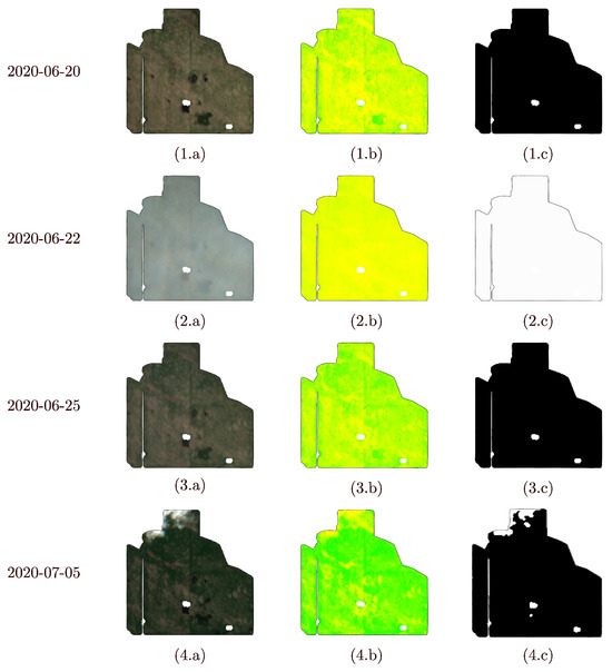
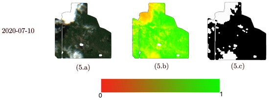 Figure 1. RGB image (column a), NDVI image V (column b) and obstruction matrix M (column c) for a selection of days between 20 June 2020 and 10 July 2020. 20 June 2020 and 25 June 2020 are examples of days with no obstructions. 5 July 2020 and 10 July 2020 are examples of type 1 obstructions (partial obstructions), and 22 June 2020 is an example of type 2 obstruction (full obstruction). In NDVI images, the NDVI values are proportionally mapped to a colormap ranging from green to red.
 - Fully missing NDVI images: The most common scenario of this type occurs when obstructions completely cover the AZ, resulting in all elements of the M matrix for the AZ having a value of 1, indicating total invalidation. An example of this is shown in Figure 1 (22 June 2020). Similarly, the scenario where the satellite fails to capture the AZ due to temporal resolution limitations can also be classified under this type.
For type 1 images (with partial obstructions), in addition to a temporal approximation, we can utilize valid pixels outside of the ROI. This is feasible as nearby pixels are usually expected to have similar values. Spatial approximation methods rely on valid nearby pixels to estimate the value of the invalid pixels. Additionally, by combining spatial and temporal approximation methods, we can achieve better results.
For type 2 images, we cannot directly use the spatial approximation method as we do not have other valid pixels in the AZ to rely on; we can only use temporal approximations. However, the improvements made in the type 1 images of other days can implicitly enhance the temporal approximations.
These methods operate on a set of images captured from the same location. Let represent a series of satellite images taken over a fixed period, sorted by date in ascending order. Sentinel-2 satellites have a revisit time of 3 to 5 days, resulting in a maximum of 121 images per year in S. For each image in the S, a corresponding NDVI image is generated using the NDVI Equation (1).
This process generates the series , where is the NDVI image corresponding to .
3.3. Spatial Approximation
As discussed in Section 3.2, two types of obstructions must be addressed: type 1, partially obstructed images and type 2, fully obstructed images. Spatial approximation methods are only applicable for approximating invalid pixels in type 1 images, as these methods rely on the availability of surrounding valid pixels in .
Various spatial approximation methods can be utilized for this task. Siravenha et al. (2011) have tested two families of spatial approximation methods, namely nearest neighbour methods and variational methods, which result in a partial differential equation-based approach [64]. In this work, we adapt the second-order partial differential equations, specifically the Laplacian inpainting method, which has been reported as a highly effective technique in previous studies [64]. The Laplacian method is also a widely used technique in image restoration due to its ability to preserve smooth transitions across pixels. This property aligns well with the characteristics of the farm field images, where gradual variations between neighbouring regions are expected.
Let I represent the NDVI image for a day affected by a type 1 obstruction. To reconstruct the missing NDVI values within the region of interest (), we employ the Laplacian method. By solving the Laplace equation, we ensure a smooth reconstruction that minimizes deviations from the values at the boundary of () (see Figure 2).
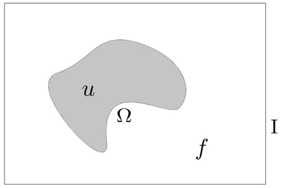
Figure 2.
The function f represents the available NDVI values in the image I, which are missing within the region of interest . Inside , u denotes the function that approximates these missing values.
Let f represent the NDVI values for I in . The function f is defined and known outside , but its values are missing within . To approximate the missing values, we seek an approximating function u that matches f along the boundary of .
The Laplacian equation forms the foundation of this approximation. The goal is to minimize the variation of u by minimizing the variation metric over , represented as:
where ∇ denoted the gradient operator, and represents the spatial coordinates. Using principles from the calculus of variations, solving this minimization problem corresponds to finding a function u that satisfies the associated Euler-Lagrange equation [65]. In the case of Equation (2) the resulting equation is the Laplace equation:
subject to the Dirichlet boundary condition:
where is the Laplace operator. This ensures that the reconstructed values within vary smoothly from the known values along the boundary.
The Laplace equation with the Dirichlet boundary condition,
defined on the images, can be converted into a linear system of equations. The resulting system can then be solved efficiently to approximate u within . For 2D images, the discrete Laplace operator at a pixel is defined in term of the neighbourhood pixels:
To solve the Laplace equation with Dirichlet boundary conditions on a discretized domain , we construct a linear system of size , where r corresponds to the number of pixels located within or on the boundary of . Each row of the system encodes the Laplacian weights for a specific pixel, as defined in Equation (4). For improved structure and computational efficiency, the unknown (interior) pixels can be ordered first, followed by the known (boundary) pixels [66]. This formulation enables efficient solution of the Laplace system using sparse linear algebra techniques:
where
is the discrete Laplacian matrix for all involved pixels and
represents the pixels values. Here, corresponds to the values of pixels inside , and corresponds to the values of pixels on the boundary of ().
Equation (5) simplifies to:
This system forms a sparse matrix, which, with an appropriate mapping, can be transformed into a banded matrix for efficient implementation [67]. The mapping involves converting the 2D pixel coordinates into a 1D index k by assigning each pixel a unique index based on its position in the image grid. For instance, in an image with dimensions , a row-wise mapping can be utilized, following the rule:
Figure 3 shows an example of the Laplacian method applied to an NDVI image.
Figure 3.
Visualization of the Spatial (Laplacian) method applied to an NDVI image. (a) shows the obstruction-free ground truth, while (b) introduces artificial obstructions used as input for the spatial approximation method. (c) presents the result of the spatial approximation. The visualization is produced by proportionally mapping NDVI values to a red-green colour map as demonstrated by the accompanying legend.
3.4. Temporal Approximation Using Non-Uniform B-Splines
There are many effective curve-fitting techniques available for temporal approximations [41,42,43,44,55,56]. We aim to use a method that is simple and explicit, allowing it to be seamlessly combined with spatial approximations to form the basis of our spatiotemporal model for NDVI. Due to missing data caused by clouds, shadows, and temporal resolution limitations, we prefer a curve model that offers sufficient flexibility to control time spans. Therefore, we use non-uniform B-Spline models, which provide versatility in adjusting control points, knot values, and their degrees. Control points are the points that define the shape of the B-Spline curve; knot values are the parameters where basis functions are joined; and degree refers to the polynomial order of the basis functions (e.g., cubic for degree 3) [47]. The non-uniformity of the knot values provides flexibility, allowing for dynamic adjustment of the time spans to accommodate the irregular patterns found in the available temporal data. Additionally, the locality of the basis functions can be leveraged for efficient computation and better representation of localized variations in the NDVI data.
The temporal approximation utilizes pixel values over time to estimate the missing values in . Let represent the NDVI values at pixel for various dates, derived from the available NDVI images while excluding missing values based on M (see Section 3.2).
This time series serves as the input to our temporal method, representing the values of the same pixel position throughout the analysis period (one year, in this case). The primary objective of the temporal method is to estimate y for any specified d. Figure 4 illustrates this time series, showcasing the variations in NDVI values at a single pixel over time. Rather than directly using d as the variable for y, we adopt a more general parameter domain, represented by the variable t, and focus on approximating (as shown in Figure 4).
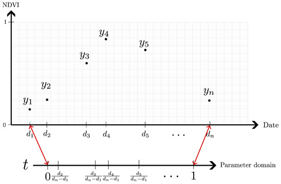
Figure 4.
An example of Y time series, plotted using NDVI-Data axis, with the d to parametric domain t mapping.
3.4.1. Constructing Non-Uniform B-Splines for Temporal Variations
We employ non-uniform B-Splines for approximating . The general form of a B-Spline function is given by:
where denotes the control points, p represents the order of the B-Spline, and are the basis functions. These basis functions are defined recursively as:
where refers to the knot sequence . The first-order B-Spline, which serves as the base case for the recursive definition, is defined as:
To construct the B-Spline curve for approximating the NDVI function, both the knot sequence and the control points are required. In this work, we utilize a least squares curve fitting problem based on the data Y:
In this minimization problem, there is an additional unknown to be resolved: the parameter values , which correspond to the available dates (i.e., ). We employ a simple proportional relationship for this:
as illustrated in Figure 4. Furthermore, rather than incorporating the knot sequence directly into the optimization model in (9), we can enforce a predefined distribution for the knot sequence based on the pattern of available dates in the data. While satellite images are typically captured at regular intervals, obstructions—such as those caused by cloud cover—can vary significantly depending on the time of year and location. For example, cloud cover in December is often drastically different from that in August, particularly in the Canadian Prairies.
We propose a method to distribute the knot sequence based on the data pattern, ensuring a more predictable and robust optimization process (refer to Section 3.4.2). Including the knot sequence directly within the optimization model, however, transforms the problem into a non-linear one, which is computationally less efficient compared to the linear model derived from least squares minimization for determining the control points.
Using a low-order B-Spline function, such as or , is preferred due to its efficient construction. Moreover, the basis functions exhibit compact support, allowing for more localized modifications influenced by the control points.
Determining the number of control points m for the B-Spline curve in relation to the number of available NDVI data points n depends on several factors, including the desired smoothness, flexibility of the results, and the expected NDVI pattern shapes influenced by the phenology of crop and vegetation growth [68]. If m is excessively large (in the extreme case where , the curve essentially becomes an interpolation of the data points), it may capture noise within the data and exhibit highly oscillatory or wiggly behavior. This pattern can be seen in Figure 5, where the curve with 30 control points demonstrates oscillatory patterns. On the other hand, if too few control points are used, the model may fail to approximate the data accurately due to an insufficient number of parameters for optimization, as shown in panel (a) of Figure 5. Hence, it is logical to define the number of control points as being proportional to the number of data points:
where D is a constant representing the number of data points per control point. Our experimental results suggest that D around 9 or 10 provides a good balance (see panel (b) in Figure 5).
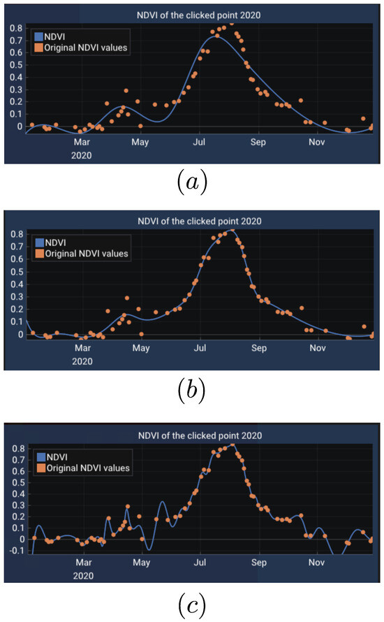
Figure 5.
An example of the effect of the number of control points chosen for B-Spline on the shape of the final curve. The figures show the B-Spline approximation curve on the data of a single pixel in 2020 using (a) 6 control points (b), 18 control points (c), and 30 control points. The curve in (a) cannot capture the trend of the data well. The panel (b) captures the expected behaviour of NDVI. (c) Shows overfitting and oscillatory behaviour due to having too many control points, as a result, capturing the inherent noise in the data as well.
3.4.2. Dynamic Knot Sequence Distribution
The common approaches for fitting B-Splines typically involve either using a predefined uniform distribution or incorporating the knot sequence into the optimization model [47]. However, when approximating NDVI values, the knot sequence can be dynamically adjusted to reflect the availability of the data.
The core idea of our method is to enforce D units in the knot space by stepping through the available dates . This process is formalized in Algorithm 1, which specifies the knot sequence distribution.
| Algorithm 1 Temporal approximation and dynamic knots |
 |
3.4.3. Solving the Least Squares Problem for Control Points
With the knot sequence determined using Algorithm 1 and the parameter values obtained (Equation (10)), we can solve the least squares problem (9) to compute the set of control points [14]. This results in a banded linear system, which can be solved efficiently using the banded Cholesky factorization method [67].
The examples shown in Figure 6 were derived using this method.
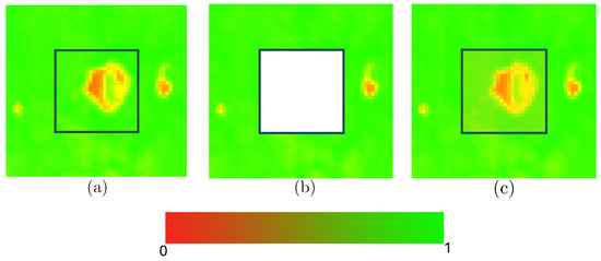
Figure 6.
Visualization of the Temporal (B-Spline) method applied to an NDVI image. (a) shows the obstruction-free ground truth, while (b) introduces artificial obstructions used as input for the temporal approximation method. (c) presents the result of the temporal approximation. The visualization is produced by proportionally mapping NDVI values to a red-green colourmap as demonstrated by the accompanying legend.
3.5. Spatiotemporal Model Based on Distance Transform
In the previous two subsections, we discussed the application of Laplacian and B-Spline methods for reconstructing missing sections of NDVI images. By combining these approaches, a more robust Spatiotemporal model for NDVI can be developed, enabling greater accuracy in the reconstruction of missing data.
To estimate the missing NDVI values at () for the date , we start by using a linear combination of the spatial approximation and the temporal approximation as follows:
where is a weighting factor that controls the relative influence of the spatial and temporal components. Setting the results in the “simple combination” method, where we average out the result of temporal and spatial approximation without considering any other factors.
However, this simple blending has limitations. Although provides a highly accurate approximation near the boundary of , its accuracy decreases for points further from the boundary as approximation errors tend to accumulate. This behavior is visualized in Figure 7, where the error increases with distance from the boundary.
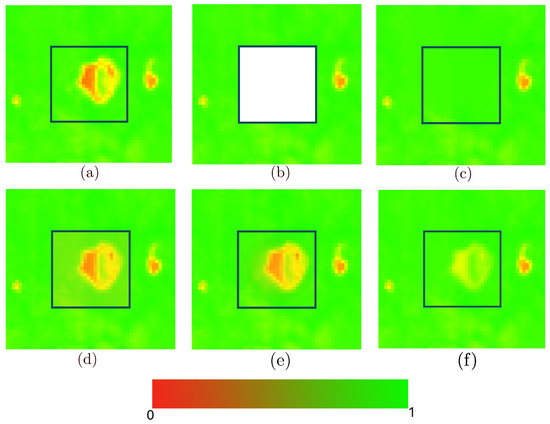
Figure 7.
Comparison of Temporal (B-Spline), Spatial (Laplacian), and distance-transform-based spatiotemporal methods on an NDVI image. (a) represents the obstruction-free ground truth, while (b) introduces artificial obstructions used as input for all methods. Results include the spatial method with RMSE of 0.0372 (c), the temporal method with RMSE of 0.0156 (d), our distance-based Spatiotemporal method with RMSE of 0.0118 (e) and the simple Spatiotemporal model (f).
To address this issue, we propose a more advanced model that varies w dynamically based on the distance of x to the boundary of . This requires calculating the distance of each point within from its boundary. The distance transform operation [69] provides a systematic and efficient solution to achieve this computation. Figure 8 illustrates the result of applying the distance transform to a square-shaped missing region.
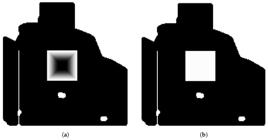
Figure 8.
Visualization of an artificial and the distance transform of that . (a) Distance Transform of , (b) .
In our ultimate model, the weight w is defined as a function of the distance of x from the boundary of :
where represents the distance of x from .
The weight function w must be defined such that , ensuring complete reliance on the spatial approximation near the boundary, and for , where L represents the maximum allowable distance for applying the spatial approximation, thereby restricting its range.
To achieve optimal performance for NDVI data across various regions and fields, it is essential to control the behavior of w (as a decay function), including the parameter L. To this end, we introduce a flexible representation of w using Bézier curves, enabling precise tuning and adaptability to real-world data.
Constructing the Decay Function
To construct the decay function w, our goal is to achieve a smooth, monotonic transition from 1 to 0—or, more broadly, from spatial to temporal approximations—with explicit control over both the rate of change and the behavior near the endpoints. Smoothness is essential for avoiding artifacts during blending, as it ensures that the transition between the interior and exterior of the domain is as seamless as possible. It is also important to include parameters that allow control over the rate of change or flatness at the beginning and end of the decay function. In general, simple and controllable parametric curves are well-suited for this purpose. We adopt a cubic Bézier curve due to its ideal balance of analytic simplicity, computational efficiency, and parametric flexibility. Unlike other monotonic functions, such as the double sigmoid or hyperbolic tangent, the Bézier formulation enables:
- Explicit control of flatness and smoothness at the endpoints
- Flexible shape adjustment via control points of a low-degree polynomial curve
Quadratic Bézier curves lack the necessary degrees of freedom to provide meaningful control over both the transition shape and endpoint behavior. Conversely, higher-degree Bézier curves offer additional control points but introduce increased computational complexity and may suffer from unwanted oscillations or reduced stability, particularly when precise localized adjustments are needed.
To define the cubic Bézier curve, four control points—, , , and —must be specified. To preserve the general structure of the decay function, the first control point is set to , and the last control point is set to . The tangent at the starting point is determined by , while at the endpoint , it is governed by (see Figure 9). Positioning on the line and on the line ensures that the tangents are horizontal at both endpoints. The x-coordinates of and control the flatness of the curve near the beginning and the end, providing flexibility in constructing the decay function. This flexibility will be leveraged in Section 4 to determine optimal parameters for a range of cloud and shadow patterns.
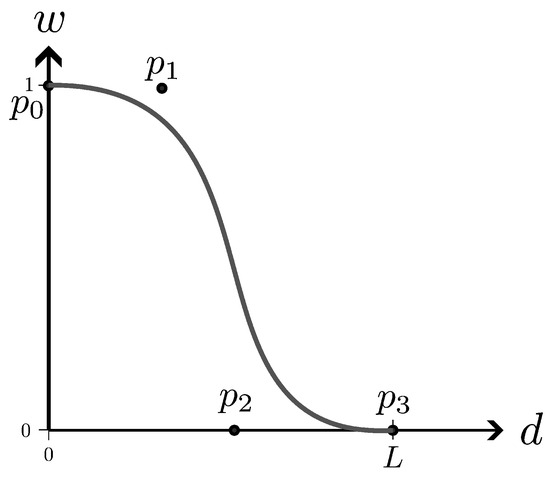
Figure 9.
Cubic Bézier curve used as the weight function , with control points , , , and , ensuring zero tangents at and . This smoothly transitions the weighting from spatial () to temporal () approximations over the d. The black line indicates the Bézier curve. is set at L, which is the distance threshold where we switch from a weighted combination to using the temporal solution only.
To guarantee that the resulting Bézier curve is a decreasing function, we impose the condition , which restricts the feasible parameter space.
With the decay function in place, the construction of our proposed distance-transform-based spatiotemporal model, as defined in Equation (13), is now complete. From this point forward, we will use the terms ‘distance-based’ and ‘distance-transform-based’ interchangeably. In the next section, we rigorously evaluate our model performance and apply it to a case study.
4. Results and Evaluations
This section presents the results of our spatiotemporal model alongside their corresponding evaluations, with an emphasis on the accuracy of the approximations. Additionally, we showcase the application of this model through a case study in precision agriculture, where it is employed to determine the peak green day for agricultural fields.
To evaluate the model’s performance, the results of the construction are compared against known ground truth, providing a reliable measure of its accuracy. For this assessment, obstruction-free NDVI images are utilized, and obstruction masks are systematically introduced to synthesize . The model’s output for the synthesized is then compared to the ground-truth images. The accuracy of the approximation is quantified using Root Mean Square Error (RMSE), which measures how closely the approximations align with the true values of the function f on .
4.1. Data
One critical challenge in ensuring fair evaluation is the selection of patterns used to synthesize , as these patterns can influence the performance of the methods. Furthermore, the parameters of the exact form of the decay function (see Section 3.4.2) must be derived from these patterns. To address this, rather than relying on arbitrary obstruction patterns, we leverage a dataset of real-world cloud and shadow patterns.
This dataset is derived from 16 farm fields located in Western Canada, primarily within the provinces of Alberta and Saskatchewan. The bounding boxes for all 16 fields are provided in the Supplementary Material. A subset of five tested fields is illustrated in Figure 10. Notably, several of these fields exhibit considerable complexity. Field #5 and Field #12, for instance, feature heterogeneous land cover, irregular boundaries, and spatial discontinuities. This complexity is further amplified by the presence of cloud formations exemplified in panel (5.c) of Figure 1. Despite these challenges, our method demonstrates robust performance and maintains reconstruction accuracy across such visually and structurally demanding scenarios. As illustrated in Figure 11, the reconstruction of Field #12 and Field #5 achieves a low RMSE, underscoring the method’s resilience in handling both spatial and atmospheric variability.
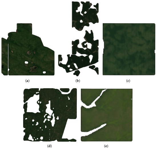
Figure 10.
5 of the 16 fields used for testing. (a) Field #1, (b) Field #5, (c) Field #8, (d) Field #12, (e) Field #13.
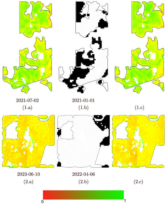
Figure 11.
Examples of reconstruction in complex fields from the 16 Canadian fields dataset under challenging cloud patterns. Top row (Field #5) and bottom row (Field #12): (Column a) shows the NDVI image from a cloud-free day; (Column b) shows a cloud mask from a different day; (Column c) shows the reconstructed NDVI image after applying the cloud mask in (column b) to the clear NDVI in (column a) using the proposed distance-transform-based spatiotemporal method.
Additionally, to enhance the geographical diversity of the test areas, the one field in Scotland and one in India used in the work of Czerkawski et al. has also been added to the dataset, with roads and buildings removed using a low variation filter [70]. Also, a selection of patterns from the 16 Canadian fields is included in the Supplementary Material. For each field, we compiled all available satellite images taken between 1 January 2018, and 30 December 2023. These images were sourced from the Sentinel-2 platform (through Sentinel-Hub, https://www.sentinel-hub.com/, (accessed on 12 November 2024)), specifically Level-2A atmospherically corrected products at 10 m ground resolution for the bands used in NDVI calculation (Band 4: red, Band 8: NIR). Each field yielded approximately 110–150 images annually over the 6-year period (varying due to orbital coverage and data availability). The nominal revisit time is 5 days at the equator and 2–3 days in mid altitudes, which include Canada, but usable images were reduced by cloud cover (average of 55.10% of initial images were clear or partially clear images after initial filtering). Cloud masks were generated using the method proposed by Layton et al. [71] with no extra buffering, as they use a statistical model to extend the cloud-shadow map with better accuracy, which eliminates the need to extend the map with a buffer.
To establish the set of ground-truth images, obstruction-free images, referred to as clear days , are first identified. Each image in is then paired with the masks extracted from all cloudy days. Specifically, the M matrix from the cloudy images is applied to the clear images to create a synthesized for these days.
4.2. Comparing Spatial, Temporal and Spatial Temporal Methods
In this subsection, we compare the distance transform-based model (13) with purely temporal, purely spatial, simple Spatiotemporal models and a machine learning model. The B-Spline, Laplacian, simple combination, and distance-based methods are all implemented as described in the methodology section. Savitzky-Golay filtering is implemented based on [10]. Spatiotemporal Kriging is performed using [72] with the OrdinaryKriging3D option and a linear variogram model. For ConvLSTM, we modified an implementation from [55] available at [73] to use only NDVI images and their dates as inputs. This modification ensures that ConvLSTM is on the same footing as the other methods. The date data is incorporated as a dense vector. For the distance-based model, it is first necessary to determine the optimal x-coordinates of and within the decay function. As discussed in Section 3.4.2, the relationship must hold. Additionally, it is crucial to determine the parameter L, which represents the decay length. L can be defined in terms of the maximum distance of points within , denoted as , and it must satisfy the condition . To approximate the optimal values, we discretize the range of to into approximately 30 intervals and L into 10 bins. We then exhaustively evaluate all possible forms of the decay functions across the obstruction patterns for each field. Following this, we compute and assess the average RMSE error across all fields and all available years, providing a comprehensive evaluation of the model’s performance. We also did the same processes for the India and Scotland fields. Table 1 shows the results of this evaluation.

Table 1.
RMSE of each method over all the 16 Canadian fields collected in six years (2018–2023), India and Scotland.
The process of exhaustively searching for the optimal values of , , and L is computationally expensive, as all possible combinations of , , and L need to be tested. A fixed set of parameter values can be determined to develop a more practical approach and eliminate the need for exhaustive searches. This means rather than defining a decay function specific to each field, we can adopt a standardized and constant decay function that applies uniformly across all fields.
The core idea is to apply the same process used for a single field across all fields and years, then compute the average of the resulting values. Through this approach, we determined that , and .
Table 2 presents a comparison between applying a variable decay function tailored to each field and a standardized (constant) decay function applied uniformly across all 16 fields. As anticipated, the variable decay function achieves a marginal improvement in accuracy; however, this comes at the expense of increased computational demands.
Table 2.
Comparison of average RMSE across all 16 Canadian fields for variational method and distance-based methods using constant and variable decay functions.
Additionally, to assess the statistical significance of these RMSE differences, we conducted independent two-sample t-tests comparing the Distance-based method against each of the baseline methods, using per-field RMSE values aggregated across years. Results, as shown in Table 3, indicate the Distance-based method significantly outperforms all baseline methods, especially the simple combination method, which is another spatiotemporal method and the ConvLSTM method, which is a deep learning approach. This confirms the observed RMSE reduction (0.0417 vs. baselines) is not due to chance, supporting the model’s efficacy in balancing spatial and temporal approximations.
Table 3.
p-value of each method against the DT method, calculated on the 16 Canadian farm fields.
The runtime characteristics of the distance-based combination method were evaluated on a consumer-grade personal computer equipped with an AMD Ryzen (TM) 7 5800X @ 4.7 GHz CPU, 32 GB of RAM running at 3200 MHz, and an RTX 3070 GPU, which was used solely for display purposes. On average, the method required 942.68 ms to reconstruct the obstructed section of a field, utilizing 789.40 MB of memory across the 16 Canadian fields. The timing data exhibited a median of 976.31 ms, with a maximum of 1357.12 ms, a minimum of 464.43 ms, a standard deviation of 63.77, and a skewness of −1.58. Similarly, for memory usage, the median was 812.38 MB, with a maximum of 986.84 MB, a minimum of 533.68 MB, a standard deviation of 49.32, and a skewness of −1.39. These results underscore the method’s computational efficiency on standard hardware, supporting its practical deployment in resource-constrained environments.
4.3. Sensitivity Analysis of Temporal Resolution
Temporal resolution can influence the performance of models with temporal components. Therefore, it is useful to explore how models such as B-Spline, simple combination, and distance-based approaches respond to changes in temporal data availability. The spatial model (Laplacian), as expected, remains unaffected by temporal resolution due to its reliance solely on spatial information.
To examine this, we conducted tests to evaluate the impact of varying temporal resolution on model performance. Initially, any image captured within 2 days before or after the test date was removed, and the tests were rerun. This process was then repeated by removing images within 4, 6, and 8 days before or after the test date, progressively decreasing the temporal data surrounding the goal date.
Table 4 present the results of this analysis for one of the test fields, highlighting the response of each model to changes in temporal resolution.
Table 4.
RMSE of each method for field #0 under varying temporal resolutions. The constant decay function uses parameters determined through an exhaustive search across all 16 fields with full temporal resolution based on data from 2018 to 2021.
4.4. Comparison with Variational-Based Spatial–Temporal Approximation
Our distance-based model (13) is constructed from simple yet efficient spatial (i.e., Laplacian) and temporal (i.e., B-Spline) components. The primary focus of this work, however, lies in exploring and analyzing the transition from spatial to temporal components in the combined model. While there are numerous ways to enhance the performance of either temporal or spatial models independently, we anticipate that integrating them through our distance-based model will yield superior results.
However, when spatial and temporal models are more interconnected, the distinction between their contributions becomes less clear. Recently, Amirfakhrian et al. introduced a variational model that leverages the temporal component to extract vector fields, which guide the reconstruction of the spatial model through a variational (i.e., Poisson) approach [36]. The interconnections between spatial and temporal components in this model make it logical to compare its results with those of our distance-based model.
Table 2 presents the comparison between their variational model and our distance-based model, which incorporates both constant and variable decay functions. The results demonstrate that our method has the potential to outperform the variational model when utilizing variable decay functions.
4.5. Comparison of Each Method’S Performance in the Presence of Cloud
A key factor influencing method performance is the extent of cloud cover in the test image. To evaluate this, we categorized cloud masks into three groups: low cloud (covering <33% of the field area), medium cloud (34–66%), and high cloud (67–95%). The 95% cutoff for high cloud excludes fully obstructed days, which would otherwise dominate and bias results toward temporal methods. Across all masks, these categories represent 38%, 26%, and 35% of cases, respectively.
Table 5 shows the RMSE for each method under these categories, averaged over the 16 fields from 2018–2023. The temporal method exhibits minimal impact from cloud amount, as it relies on NDVI-TVSI data independent of spatial obstructions. In contrast, all three spatial methods degrade sharply with increasing cloud coverage, as larger obstructions reduce available boundary information for accurate inpainting. Spatiotemporal methods are affected similarly but to a lesser degree, where the DT method handles this best, mitigating degradation through adaptive weighting that favors temporal approximations in larger gaps.
Table 5.
Average RMSE of each method over all the 16 Canadian fields collected in six years (2018–2023), separated by the cloud presence.
4.6. Comparison of Band Approximation vs. Direct Approximation
A critical consideration in our methodology is the choice to reconstruct NDVI directly from NDVI time-series data, rather than first reconstructing the underlying near-infrared (NIR) and red spectral bands and subsequently computing NDVI via Equation (1). To evaluate the differences, we tested the indirect method by using the distance-based spatiotemporal method on NIR and red bands instead of on the resulting NDVI, without altering any other aspect of the test as described in Section 4.2. Table 6 represents the result of this test on the 16 Canadian fields and shows that the direct approach has two advantages: computational efficiency and reduced error. Reconstructing individual bands requires processing multiple data layers individually, which increases memory use and processing time. Moreover, NDVI, as a normalized ratio, is sensitive to errors in the NIR and red values. Small inaccuracies in band reconstruction can be amplified through the ratio, leading to compounded uncertainties in the derived index. As such, directly approximating NDVI is the preferred approach using the proposed distance-based spatiotemporal method.
Table 6.
Comparison of characteristics of NDVI approximation over 16 Canadian fields using NDVI data as input (Direct NDVI) vs. approximating the missing areas of RED and NIR bands separately (Indirect NDVI). Both approaches use the proposed distance-based spatiotemporal method.
4.7. Case Study: Finding the Peak-Green Day in a Field
In this subsection, as a case study, we consider identifying the peak green day for fields using Sentinel-2 imagery during the growth season. The NDVI on the peak green day serves as a performance indicator for the fields. The peak green data has been utilized for various applications, including the creation of zone delineation maps for field management [19,20].
To algorithmically identify the peak green day among the available clear days = {}, we first define the ideal peak green image . This image serves as an idealized composite and does not necessarily correspond to any specific day. Each pixel in is assigned the maximum NDVI value observed for that pixel across all available images. In constructing , both clear images and cloudy images are utilized, provided the pixel in cloudy images is not obscured by their cloud mask M.
Using this definition of , the peak green day p is mathematically defined as the day whose image most closely matches the ideal image (following the approach in [19]). Specifically, p is calculated as follows:
This approach enables precise identification of the peak green day. Algorithm 2 identifies the peak-green day from an input series of NDVI images.
| Algorithm 2 Finding peak green |
 |
In practical applications, a common challenge is that many NDVI images may contain obstructions, necessitating their exclusion from the search space in Equation (14). As a result, the peak-green image is selected from a reduced subset of images, rather than the complete set of both clear and cloudy images. This restriction means that obstructions in satellite imagery can significantly influence the identification of the peak green day.
To overcome this limitation, we propose reconstructing the cloudy images using our Spatiotemporal model. By reconstructing these images, we can incorporate them into Equation (14), along with the clear images, thereby mitigating the impact of obstructions and enhancing the robustness of the peak green day estimation.
Figure 12 provides an example of the improvement achieved with this approach. Additionally, Table 7 presents the RMSE of peak green, when image is used as the ground truth. In most cases, using the distance-based spatiotemporal reconstruction provided a peak-green that is closer to the image. As shown in the table, the peak green has improved across 16 fields. For four of the fields (7, 12, 14, and 15), the peak green remains unchanged, as the images near the peak days are cloud-free.
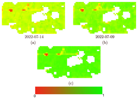
Figure 12.
An example of improved peak-green selection by using reconstructed images in field #3 in the year 2022. Image (a) is the peak-green that would have been chosen if we restricted our choice to clear day images, (b) is the peak-green resulting from the complete set of both clear and reconstructed cloudy images using the distance-based spatiotemporal method, and (c) is the ID image. The visualization is achieved by proportionally mapping NDVI values to a red-green colourmap, similar to Figure 3.
Table 7.
Comparison of average RMSE regarding the difference of the chosen image as peak-green and the image, using the data from the year 2020. Other than fields 7, 12, 14 and 15, in all other cases, we can see an improvement.
5. Discussion
The proposed spatiotemporal distance-based combination method is an NDVI approximation algorithm, meant to be used for agricultural fields, where the computational budget is limited. Our approach introduces a novel integration of distance transform logic, including the parametric decay function, within a spatiotemporal framework—a combination that, to our knowledge, is not present in any existing method. This design enables the model to simultaneously leverage spatial proximity and temporal continuity, offering a computationally efficient, interpretable, and low-overhead alternative to more complex machine learning approaches.
The majority of recent research utilizes multiple satellite data and combines them using machine learning methods to obtain an accurate approximation of NDVI. This results in the need for specialized hardware and considerable computational resources, such as memory and time to process. In contrast, our proposed method works using a single data source (calculated NDVI using one satellite’s images) and needs less than 1 s to process and less than 800 MB of memory on a conventional consumer-grade computer. Unlike many existing techniques that rely on extensive training data or intricate parameter tuning, our model is lightweight and interpretable to the end user, making it well-suited for operational deployment in smart agriculture workloads. We tested this method on 16 fields in Western Canada, Scotland, and India, and demonstrated its effectiveness compared to other methods that utilize only one data source and have similar hardware and processing needs to our proposed method.
The proposed spatiotemporal distance-based combination method is reliant on the performance of the underlying temporal and spatial methods used. We tested two scenarios where the performance of one method is decreased, with minimal effect on the other method. In Table 4 and Table 5, we can see the result of the tests that decreased the performance of the temporal and spatial method respectively and the result shows that the distance-based method although is reliant on the effectiveness of its underlying methods, it still manages to stay more effective than the affected method itself. One notable observation, using the variable decay approach, is that when temporal resolution is higher, the temporal model performs better, and the transition from spatial to temporal components can occur more rapidly. Conversely, when temporal resolution is extremely low, the spatial component becomes more reliable, allowing the transition to progress more gradually. Similarly, in low cloud situations, the result of the spatial method is more accurate, which means that reliance on the spatial method is needed.
The Bézier curve, used for the combination weight function, has a set of 3 parameteres that can determine its efficacy as well. We propose two methods of obtaining the parameters based on the data. The choice between these methods depends on the specific use case. The variable decay function is ideal for scenarios requiring maximum accuracy, particularly when computational resources are not a constraint. On the other hand, the constant decay function offers a practical and efficient alternative for large-scale applications where computational efficiency is prioritized over slight accuracy gains. The difference between the effectiveness of these methods is shown in Table 2. Our empirical method for determining the decay function is based on the dataset derived from Sentinel-2. Consequently, for other datasets—especially those with spatial and temporal resolutions significantly different from Sentinel-2— the decay function should be re-evaluated using the approach outlined in Section 4.2.
Our method operates effectively throughout the typical growing season in the Northern Hemisphere, spanning from early spring to mid-fall. During this period, agricultural landscapes undergo substantial changes in vegetation structure, soil exposure, and spectral characteristics due to crop emergence, maturation, and harvest cycles. The proposed approach demonstrates resilience to these seasonal variations, maintaining reconstruction accuracy despite shifts in texture, colour, and canopy density. Although our focus is on this seasonal window, the method is not geographically constrained and can be applied to Southern Hemisphere regions by aligning with their respective agricultural calendars. While validation on off-season imagery remains a direction for future work, it was not necessary for this study or its intended applications.
6. Conclusions
The proposed distance-based spatiotemporal model demonstrates a robust, simple, and effective approach for approximating NDVI in scenarios where cloud and shadow contamination limit the analysis. By integrating spatial and temporal components through the distance transform and the newly introduced decay function, the model achieves significant improvements in accuracy compared to standalone or simple combined methods, as evidenced by RMSE evaluations. Unlike machine learning-based methods, which often require large labeled datasets, extensive computational resources, and complex parameter tuning, our model offers a straightforward and interpretable solution. This simplicity makes it more accessible, practical, and directly applicable to scenarios where data availability or computational capacity is limited. The results, derived from testing across 16 farm fields in Western Canada, confirm the model’s capability to address practical challenges in vegetation analysis. Furthermore, the application of this model to refining the specification of peak green day highlights its potential for broader agricultural monitoring applications.
The strength of our proposed distance-transform-based approach lies not merely in the specific spatial or temporal approximation techniques it employs, but in its robust capacity to seamlessly integrate these components into a unified model that outperforms either in isolation.
As possible directions for future work, investigating more dynamic and adaptive decay functions that account for larger datasets with more spatial and environmental variations could be considered. This may require more advanced optimization methods and potentially leveraging machine learning techniques to complement the model’s foundational framework.
Expanding the proposed model to address missing data in other spectral indices, applicable across various domains and use cases, presents a compelling opportunity for future research.
Finally, our analysis demonstrates that the simple distance-based spatiotemporal model, when paired with an appropriately designed decay function, performs at a level comparable to advanced variational models, such as the Poisson model. Moreover, our findings indicate that with a carefully chosen decay function, the performance of the distance-based model can exceed that of the variational model. This serves as a strong indication of the potential for further enhancement and refinement. A promising future direction could involve investigating the practical and efficient integration of the distance transform and decay function with variational methods, aiming to achieve even greater performance and broaden the model’s applicability.
Supplementary Materials
The following supporting information can be downloaded at: https://www.mdpi.com/article/10.3390/rs17203399/s1.
Author Contributions
Conceptualization, A.M., M.A. and F.F.S.; Methodology, A.M. and F.F.S.; Software, A.M. and L.W.; Validation, A.M.; Formal analysis, A.M. and F.F.S.; Investigation, A.M.; Resources, F.F.S.; Data curation, A.M. and L.W.; Writing—original draft, A.M. and M.A.; Writing—review & editing, A.M., L.W. and F.F.S.; Visualization, A.M.; Supervision, F.F.S.; Project administration, F.F.S. All authors have read and agreed to the published version of the manuscript.
Funding
This research was funded by MITACS, TELUS Agriculture, Application Ref. IT32167.
Data Availability Statement
No new data were created or analyzed in this study. Data sharing is not applicable to this article.
Acknowledgments
We gratefully acknowledge the support from the Mathematics of Information Technology and Complex Systems (MITACS), Decisive Farming (TELUS Agriculture), and the Natural Sciences and Engineering Research Council of Canada (NSERC). We’d also like to extend our thank to the full GIV research team at the University of Calgary for their insights and dynamic discussions throughout this project.
Conflicts of Interest
The authors declare no conflicts of interest.
References
- Mulla, D.J. Twenty five years of remote sensing in precision agriculture: Key advances and remaining knowledge gaps. Biosyst. Eng. 2013, 114, 358–371. [Google Scholar] [CrossRef]
- Berger, A.; Ettlin, G.; Quincke, C.; Rodríguez-Bocca, P. Predicting the Normalized Difference Vegetation Index (NDVI) by training a crop growth model with historical data. Comput. Electron. Agric. 2019, 161, 305–311. [Google Scholar] [CrossRef]
- Pettorelli, N. The Normalized Difference Vegetation Index; Oxford University Press: Oxford, UK, 2013. [Google Scholar] [CrossRef]
- Gao, F.; Masek, J.; Schwaller, M.; Hall, F. On the blending of the Landsat and MODIS surface reflectance: Predicting daily Landsat surface reflectance. IEEE Trans. Geosci. Remote Sens. 2006, 44, 2207–2218. [Google Scholar]
- Zhu, X.; Chen, J.; Gao, F.; Chen, X.; Masek, J.G. An enhanced spatial and temporal adaptive reflectance fusion model for complex heterogeneous regions. Remote Sens. Environ. 2010, 114, 2610–2623. [Google Scholar] [CrossRef]
- Zhu, X.; Helmer, E.H.; Gao, F.; Liu, D.; Chen, J.; Lefsky, M.A. A flexible spatiotemporal method for fusing satellite images with different resolutions. Remote Sens. Environ. 2016, 172, 165–177. [Google Scholar] [CrossRef]
- Li, J.; Li, C.; Xu, W.; Feng, H.; Zhao, F.; Long, H.; Meng, Y.; Chen, W.; Yang, H.; Yang, G. Fusion of optical and SAR images based on deep learning to reconstruct vegetation NDVI time series in cloud-prone regions. Int. J. Appl. Earth Obs. Geoinf. 2022, 112, 102818. [Google Scholar] [CrossRef]
- Abdelaziz Htitiou, A.B.; Benabdelouahab, T. Deep Learning-Based Spatiotemporal Fusion Approach for Producing High-Resolution NDVI Time-Series Datasets. Can. J. Remote Sens. 2021, 47, 182–197. [Google Scholar] [CrossRef]
- dos Santos, E.P.; da Silva, D.D.; do Amaral, C.H.; Fernandes-Filho, E.I.; Dias, R.L.S. A Machine Learning approach to reconstruct cloudy affected vegetation indices imagery via data fusion from Sentinel-1 and Landsat 8. Comput. Electron. Agric. 2022, 194, 106753. [Google Scholar] [CrossRef]
- Chen, J.; Jönsson, P.; Tamura, M.; Gu, Z.; Matsushita, B.; Eklundh, L. A simple method for reconstructing a high-quality NDVI time-series data set based on the Savitzky–Golay filter. Remote Sens. Environ. 2004, 91, 332–344. [Google Scholar] [CrossRef]
- Heuvelink, G.B.; Pebesma, E.J. Spatial aggregation and soil process modelling. Geoderma 2006, 140, 351–361. [Google Scholar] [CrossRef]
- Chan, T.F.; Shen, J. Nontexture Inpainting by Curvature-Driven Diffusions. J. Vis. Comun. Image Represent. 2001, 12, 436–449. [Google Scholar] [CrossRef]
- Bertalmio, M.; Sapiro, G.; Caselles, V.; Ballester, C. Image inpainting. In Proceedings of the 27th Annual Conference on Computer Graphics and Interactive Techniques (SIGGRAPH ’00), New Orleans, LA, USA, 23–28 July 2000; pp. 417–424. [Google Scholar] [CrossRef]
- Samavati, F.F.; Amiri, N.M. A Filtered B-spline Model of Scanned Digital Images. J. Sci. Islam. Repub. Iran 1999, 10, 258–264. [Google Scholar]
- Aguilera, A.; Aguilera-Morillo, M. Comparative study of different B-spline approaches for functional data. Math. Comput. Model. 2013, 58, 1568–1579. [Google Scholar] [CrossRef]
- Eilers, P.H.C.; Marx, B.D. Flexible smoothing with B-splines and penalties. Stat. Sci. 1996, 11, 89–121. [Google Scholar] [CrossRef]
- Eilers, P.H.C.; Marx, B.D. Splines, knots, and penalties. WIREs Comput. Stat. 2010, 2, 637–653. [Google Scholar] [CrossRef]
- Borgefors, G. Distance transformations in digital images. Comput. Vis. Graph. Image Process. 1986, 34, 344–371. [Google Scholar] [CrossRef]
- Heidari, R.; Samavati, F.F. A New Dissimilarity Metric for Anomaly Detection in Management Zones Delineation Constructed from Time-Varying Satellite Images. Agriculture 2024, 14, 688. [Google Scholar] [CrossRef]
- Kazemi, M.; Samavati, F.F. Automatic Soil Sampling Site Selection in Management Zones Using a Multi-Objective Optimization Algorithm. Agriculture 2023, 13, 1993. [Google Scholar] [CrossRef]
- Vélez, S.; Martínez-Peña, R.; Castrillo, D. Beyond Vegetation: A Review Unveiling Additional Insights into Agriculture and Forestry through the Application of Vegetation Indices. J 2023, 6, 421–436. [Google Scholar] [CrossRef]
- Viana, C.M.; Oliveira, S.; Oliveira, S.C.; Rocha, J. 29—Land Use/Land Cover Change Detection and Urban Sprawl Analysis. In Spatial Modeling in GIS and R for Earth and Environmental Sciences; Pourghasemi, H.R., Gokceoglu, C., Eds.; Elsevier: Amsterdam, The Netherlands, 2019; pp. 621–651. [Google Scholar] [CrossRef]
- Li, C.; Li, H.; Li, J.; Lei, Y.; Li, C.; Manevski, K.; Shen, Y. Using NDVI percentiles to monitor real-time crop growth. Comput. Electron. Agric. 2019, 162, 357–363. [Google Scholar] [CrossRef]
- Sishodia, R.P.; Ray, R.L.; Singh, S.K. Applications of Remote Sensing in Precision Agriculture: A Review. Remote Sens. 2020, 12, 3136. [Google Scholar] [CrossRef]
- Huang, S.; Tang, L.; Hupy, J.P.; Wang, Y.; Shao, G. A commentary review on the use of normalized difference vegetation index (NDVI) in the era of popular remote sensing. J. For. Res. 2021, 32, 1–6. [Google Scholar] [CrossRef]
- Yengoh, G.T.; Dent, D.; Olsson, L.; Tengberg, A.E.; Tucker, C.J. Applications of NDVI for Land Degradation Assessment. In Use of the Normalized Difference Vegetation Index (NDVI) to Assess Land Degradation at Multiple Scales: Current Status, Future Trends, and Practical Considerations; Springer International Publishing: Cham, Switzerland, 2016; pp. 17–25. [Google Scholar] [CrossRef]
- Zhao, Q.; Qu, Y. The Retrieval of Ground NDVI (Normalized Difference Vegetation Index) Data Consistent with Remote-Sensing Observations. Remote Sens. 2024, 16, 1212. [Google Scholar] [CrossRef]
- Petitjean, F.; Gançarski, P.; Masseglia, F.; Forestier, G. Analysing Satellite Image Time Series by Means of Pattern Mining. In Intelligent Data Engineering and Automated Learning—IDEAL 2010; Hutchison, D., Kanade, T., Kittler, J., Kleinberg, J.M., Mattern, F., Mitchell, J.C., Naor, M., Nierstrasz, O., Pandu Rangan, C., Steffen, B., et al., Eds.; Springer: Berlin/Heidelberg, Germany, 2010; Volume 6283, pp. 45–52. [Google Scholar] [CrossRef]
- Zhu, Z.; Woodcock, C.E. Continuous change detection and classification of land cover using all available Landsat data. Remote Sens. Environ. 2014, 144, 152–171. [Google Scholar] [CrossRef]
- Inglada, J.; Vincent, A.; Arias, M.; Tardy, B.; Morin, D.; Rodes, I. Operational High Resolution Land Cover Map Production at the Country Scale Using Satellite Image Time Series. Remote Sens. 2017, 9, 95. [Google Scholar] [CrossRef]
- Zhang, A.; Jia, G. Monitoring meteorological drought in semiarid regions using multi-sensor microwave remote sensing data. Remote Sens. Environ. 2013, 134, 12–23. [Google Scholar] [CrossRef]
- Chu, T.; Guo, X.; Takeda, K. Remote sensing approach to detect post-fire vegetation regrowth in Siberian boreal larch forest. Ecol. Indic. 2016, 62, 32–46. [Google Scholar] [CrossRef]
- Son, N.; Chen, C.; Chen, C.; Chang, L.; Minh, V. Monitoring agricultural drought in the Lower Mekong Basin using MODIS NDVI and land surface temperature data. Int. J. Appl. Earth Obs. Geoinf. 2012, 18, 417–427. [Google Scholar] [CrossRef]
- Gao, F.; Anderson, M.C.; Zhang, X.; Yang, Z.; Alfieri, J.G.; Kustas, W.P.; Mueller, R.; Johnson, D.M.; Prueger, J.H. Toward mapping crop progress at field scales through fusion of Landsat and MODIS imagery. Remote Sens. Environ. 2017, 188, 9–25. [Google Scholar] [CrossRef]
- Johnson, D.M. A comprehensive assessment of the correlations between field crop yields and commonly used MODIS products. Int. J. Appl. Earth Obs. Geoinf. 2016, 52, 65–81. [Google Scholar] [CrossRef]
- Amirfakhrian, M.; Samavati, F.F. Variational-Based Spatial–Temporal Approximation of Images in Remote Sensing. Remote Sens. 2024, 16, 2349. [Google Scholar] [CrossRef]
- Shen, J.; Chan, T.F. Mathematical Models for Local Nontexture Inpaintings. SIAM J. Appl. Math. 2002, 62, 1019–1043. [Google Scholar] [CrossRef]
- Shao, X.; Liu, Z.; Li, H. An image inpainting approach based on the Poisson equation. In Proceedings of the Second International Conference on Document Image Analysis for Libraries (DIAL’06), Lyon, France, 27–28 April 2006; pp. 368–372. [Google Scholar] [CrossRef]
- Meng, F.; Yang, X.; Zhou, C.; Li, Z. A Sparse Dictionary Learning-Based Adaptive Patch Inpainting Method for Thick Clouds Removal from High-Spatial Resolution Remote Sensing Imagery. Sensors 2017, 17, 2130. [Google Scholar] [CrossRef]
- Maduskar, D.; Dube, N. Navier–Stokes-Based Image Inpainting for Restoration of Missing Data Due to Clouds. In Proceedings of the Innovations in Computational Intelligence and Computer Vision, Jaipur, India, 5–6 August 2021; Sharma, M.K., Dhaka, V.S., Perumal, T., Dey, N., Tavares, J.M.R.S., Eds.; Springer: Singapore, 2021; pp. 497–505. [Google Scholar]
- Pan, Z.; Hu, Y.; Cao, B. Construction of smooth daily remote sensing time series data: A higher spatiotemporal resolution perspective. Open Geospat. Data Softw. Stand. 2017, 2, 25. [Google Scholar] [CrossRef][Green Version]
- Martínez, B.; Gilabert, M.A. Vegetation dynamics from NDVI time series analysis using the wavelet transform. Remote Sens. Environ. 2009, 113, 1823–1842. [Google Scholar] [CrossRef]
- Zhou, J.; Jia, L.; Menenti, M. Reconstruction of global MODIS NDVI time series: Performance of Harmonic ANalysis of Time Series (HANTS). Remote Sens. Environ. 2015, 163, 217–228. [Google Scholar] [CrossRef]
- Vorobiova, N.; Chernov, A. Curve fitting of MODIS NDVI time series in the task of early crops identification by satellite images. In Procedia Engineering, Proceedings of the 3rd International Conference “Information Technology and Nanotechnology”, ITNT-2017, Samara, Russia, 25–27 April 2017; Elsevier: Amsterdam, The Netherlands, 2017; Volume 201, pp. 184–195. [Google Scholar] [CrossRef]
- de Boor, C. On calculating with B-splines. J. Approx. Theory 1972, 6, 50–62. [Google Scholar] [CrossRef]
- Dierckx, P. Curve and Surface Fitting with Splines; Oxford University Press: Oxford, UK, 1993. [Google Scholar] [CrossRef]
- de Boor, C. A Practical Guide to Spline; Springer: New York, NY, USA, 1978; Volume 27. [Google Scholar] [CrossRef]
- Epperson, J. An Introduction to Numerical Methods and Analysis; Wiley: Hoboken, NJ, USA, 2021. [Google Scholar]
- Li, J.; Li, Y.; He, L.; Chen, J.; Plaza, A. Spatio-temporal fusion for remote sensing data: An overview and new benchmark. Sci. China Inf. Sci. 2020, 63, 140301. [Google Scholar] [CrossRef]
- Xu, L.; Li, B.; Yuan, Y.; Gao, X.; Zhang, T. A Temporal-Spatial Iteration Method to Reconstruct NDVI Time Series Datasets. Remote Sens. 2015, 7, 8906–8924. [Google Scholar] [CrossRef]
- Chen, Y.; Cao, R.; Chen, J.; Liu, L.; Matsushita, B. A practical approach to reconstruct high-quality Landsat NDVI time-series data by gap filling and the Savitzky–Golay filter. ISPRS J. Photogramm. Remote Sens. 2021, 180, 174–190. [Google Scholar] [CrossRef]
- Roerink, G.; Menenti, M.; Verhoef, W. Synthesizing cloud free NDVI composites through temporal domain analysis. Remote Sens. Environ. 2000, 75, 99–115. [Google Scholar]
- Bui, T.D.; Ravi, S.; Ramavajjala, V. Neural Graph Machines: Learning Neural Networks Using Graphs. arXiv 2017, arXiv:1703.04818. [Google Scholar] [CrossRef]
- Beyer, M.; Ahmad, R.; Yang, B.; Rodríguez-Bocca, P. Deep spatial-temporal graph modeling for efficient NDVI forecasting. Smart Agric. Technol. 2023, 4, 100172. [Google Scholar] [CrossRef]
- Ahmad, R.; Yang, B.; Ettlin, G.; Berger, A.; Rodríguez-Bocca, P. A machine-learning based ConvLSTM architecture for NDVI forecasting. Int. Trans. Oper. Res. 2023, 30, 2025–2048. [Google Scholar] [CrossRef]
- Su, Z.; Shen, J.; Sun, Y.; Hu, R.; Zhou, Q.; Yong, B. Deep Spatio-Temporal Fuzzy Model for NDVI Forecasting. IEEE Trans. Fuzzy Syst. 2024, 33, 290–301. [Google Scholar] [CrossRef]
- Makridakis, S.; Spiliotis, E.; Assimakopoulos, V. The M4 Competition: Results, findings, conclusion and way forward. Int. J. Forecast. 2018, 34, 802–808. [Google Scholar] [CrossRef]
- Elsayed, S.; Thyssens, D.; Rashed, A.; Schmidt-Thieme, L.; Jomaa, H.S. Do We Really Need Deep Learning Models for Time Series Forecasting? arXiv 2021, arXiv:2101.02118. [Google Scholar] [CrossRef]
- Candra, D.S.; Phinn, S.; Scarth, P. Cloud and cloud shadow masking using multi-temporal cloud masking algorithm in tropical environmental. Int. Arch. Photogramm. Remote Sens. Spat. Inf. Sci. 2016, 41, 95–100. [Google Scholar] [CrossRef]
- Skakun, S.; Wevers, J.; Brockmann, C.; Doxani, G.; Aleksandrov, M.; Batič, M.; Frantz, D.; Gascon, F.; Gómez-Chova, L.; Hagolle, O.; et al. Cloud Mask Intercomparison eXercise (CMIX): An evaluation of cloud masking algorithms for Landsat 8 and Sentinel-2. Remote Sens. Environ. 2022, 274, 112990. [Google Scholar] [CrossRef]
- Candra, D.S.; Phinn, S.; Scarth, P. Automated Cloud and Cloud-Shadow Masking for Landsat 8 Using Multitemporal Images in a Variety of Environments. Remote Sens. 2019, 11, 2060. [Google Scholar] [CrossRef]
- GDAL/OGR Contributors. GDAL/OGR Geospatial Data Abstraction Software Library; Open Source Geospatial Foundation: Beaverton, OR, USA, 2025. [Google Scholar] [CrossRef]
- Jiang, Z.; Huete, A.R.; Chen, J.; Chen, Y.; Li, J.; Yan, G.; Zhang, X. Analysis of NDVI and scaled difference vegetation index retrievals of vegetation fraction. Remote Sens. Environ. 2006, 101, 366–378. [Google Scholar] [CrossRef]
- Siravenha, A.C.; Sousa, D.; Bispo, A.; Pelaes, E. Evaluating Inpainting Methods to the Satellite Images Clouds and Shadows Removing. In Proceedings of the Signal Processing, Image Processing and Pattern Recognition, Jeju Island, Republic of Korea, 16–18 November 2011; Kim, T.h., Adeli, H., Ramos, C., Kang, B.H., Eds.; Springer: Berlin/Heidelberg, Germany, 2011; pp. 56–65. [Google Scholar]
- van Brunt, B. The Calculus of Variations; Universitext; Springer: New York, NY, USA, 2003. [Google Scholar]
- libigl. Laplace Equation. 2023. Available online: https://libigl.github.io/tutorial/#laplace-equation (accessed on 31 March 2025).
- Golub, G.; Kahan, W. Calculating the Singular Values and Pseudo-Inverse of a Matrix. J. Soc. Ind. Appl. Math. Ser. B Numer. Anal. 1965, 2, 205–224. [Google Scholar] [CrossRef]
- Bhatti, M.T.; Gilani, H.; Ashraf, M.; Iqbal, M.S.; Munir, S. Field validation of NDVI to identify crop phenological signatures. Precis. Agric. 2024, 25, 2245–2270. [Google Scholar] [CrossRef]
- Felzenszwalb, P.F.; Huttenlocher, D.P. Distance Transforms of Sampled Functions. Theory Comput. 2012, 8, 415–428. [Google Scholar] [CrossRef]
- Czerkawski, M.; Upadhyay, P.; Davison, C.; Werkmeister, A.; Cardona, J.; Atkinson, R.; Michie, C.; Andonovic, I.; Macdonald, M.; Tachtatzis, C. Deep Internal Learning for Inpainting of Cloud-Affected Regions in Satellite Imagery. Remote Sens. 2022, 14, 1342. [Google Scholar] [CrossRef]
- Layton, J.C.; Wecker, L.; Runions, A.; Samavati, F.F. Cloud Shadow Detection via Ray Casting with Probability Analysis Refinement Using Sentinel-2 Satellite Data. Remote Sens. 2023, 15, 3955. [Google Scholar] [CrossRef]
- Murphy, B.; Yurchak, R.; Müller, S. GeoStat-Framework/PyKrige: V1.7.2; Zenodo: Geneva, Switzerland, 2024. [Google Scholar] [CrossRef]
- Kylalangotsky (Username). ndvi_timeseries_forcasting. GitHub Repository. 2025. Available online: https://github.com/kylalangotsky/ndvi_timeseries_forcasting (accessed on 10 June 2025).


Disclaimer/Publisher’s Note: The statements, opinions and data contained in all publications are solely those of the individual author(s) and contributor(s) and not of MDPI and/or the editor(s). MDPI and/or the editor(s) disclaim responsibility for any injury to people or property resulting from any ideas, methods, instructions or products referred to in the content. |
© 2025 by the authors. Licensee MDPI, Basel, Switzerland. This article is an open access article distributed under the terms and conditions of the Creative Commons Attribution (CC BY) license (https://creativecommons.org/licenses/by/4.0/).