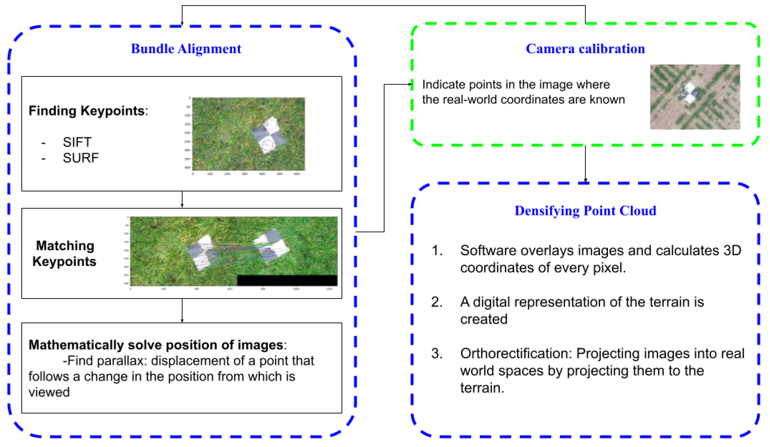
Figure 1.
Simplified diagram of some steps for the photogrammetry workflow.
Figure 1.
Simplified diagram of some steps for the photogrammetry workflow.
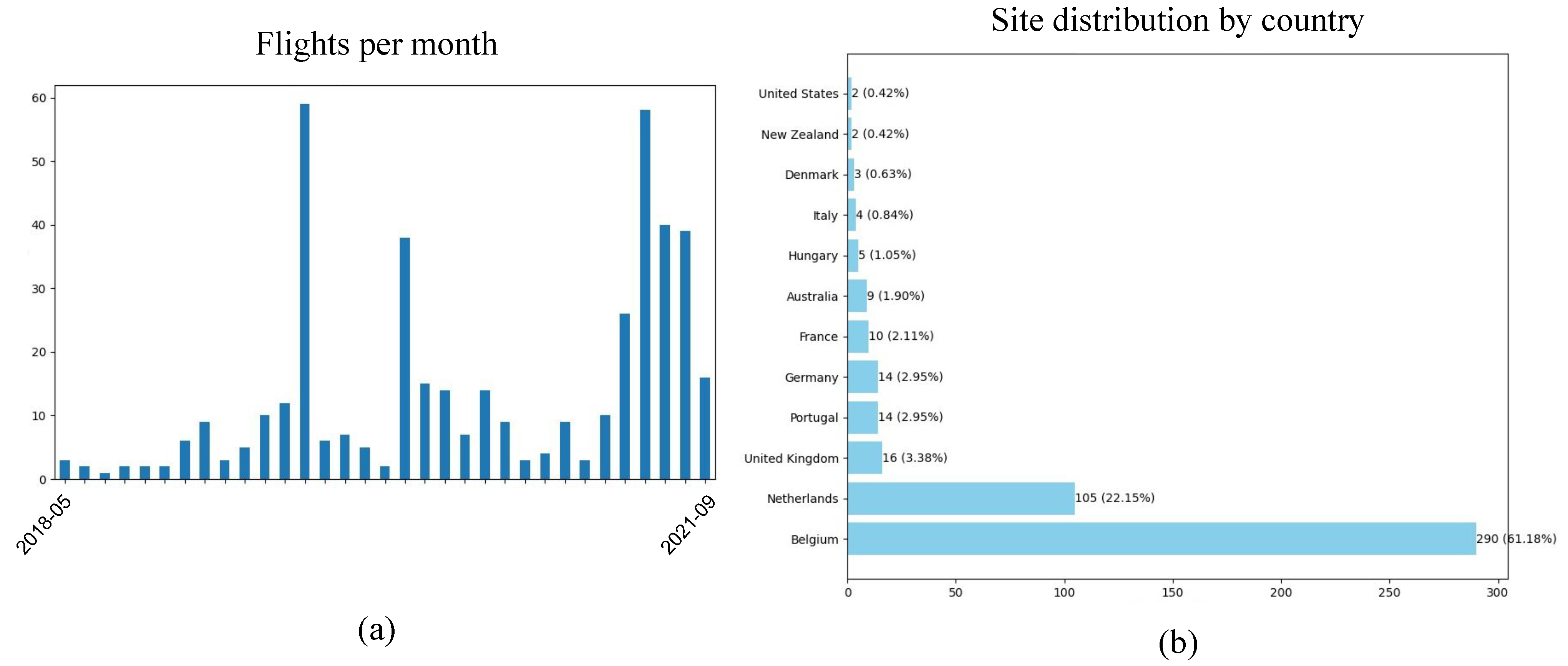
Figure 2.
Distribution of sites surveyed (a), distribution of flights per month (b).
Figure 2.
Distribution of sites surveyed (a), distribution of flights per month (b).
Figure 3.
Example of a 6016 × 4008-pixel image captured with a FC6540 with 1/100 s of exposure time, 50 mm of focal length, and 2.97 max aperture.
Figure 3.
Example of a 6016 × 4008-pixel image captured with a FC6540 with 1/100 s of exposure time, 50 mm of focal length, and 2.97 max aperture.
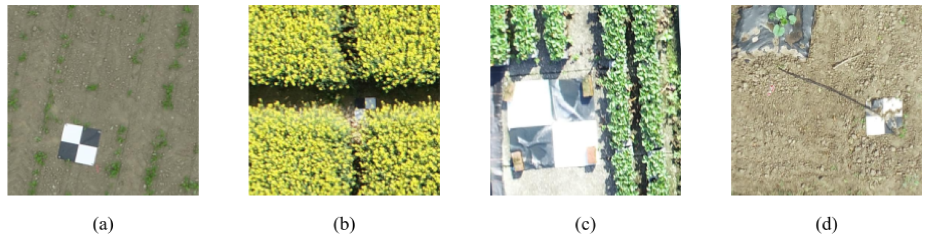
Figure 4.
Examples of 512 × 512-pixel tiles, (a) a perfectly visible GCP, (b) GCP partially covered by the crop, (c) GCP reflecting sunlight, (d) GCP covered by sand.
Figure 4.
Examples of 512 × 512-pixel tiles, (a) a perfectly visible GCP, (b) GCP partially covered by the crop, (c) GCP reflecting sunlight, (d) GCP covered by sand.
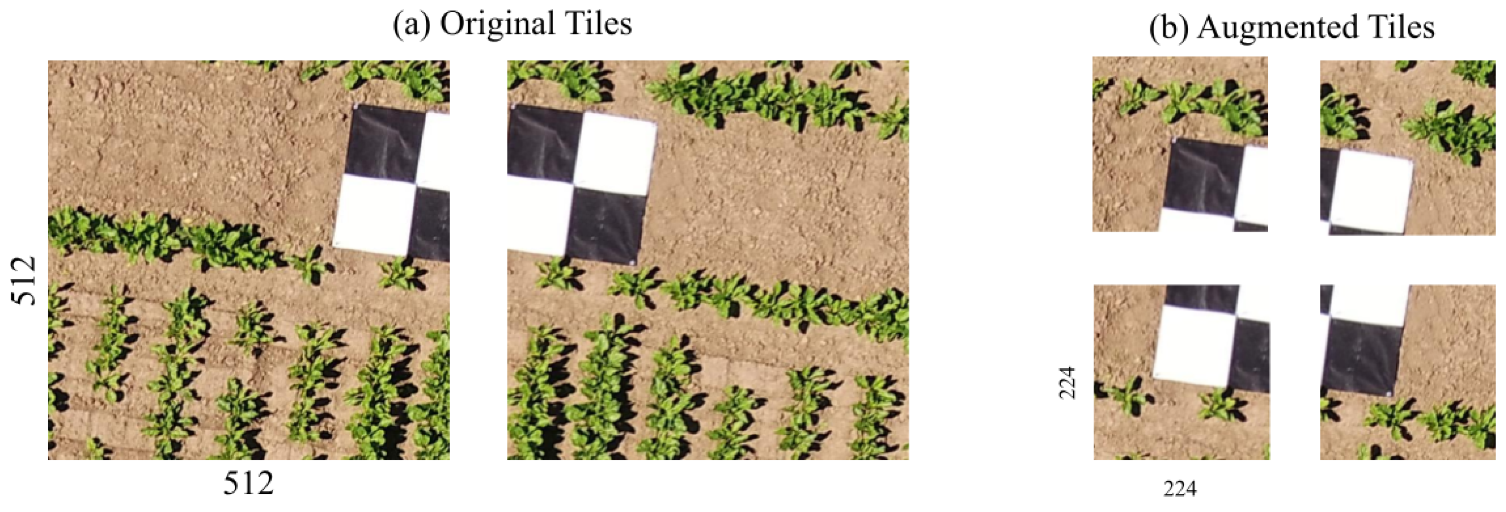
Figure 5.
Comparison of the same ground control point tiled in 512 × 512-pixel tiles, as presented by figure (a) and tiled in 224 × 224 pixel tiles as presented by figure (b).
Figure 5.
Comparison of the same ground control point tiled in 512 × 512-pixel tiles, as presented by figure (a) and tiled in 224 × 224 pixel tiles as presented by figure (b).
Figure 6.
Visual representation of the computer vision pipeline, (a) original tile, (b) binary mask with white pixels, (c) binary mask after morphological operations, (d) Canny edge detection, (e) Hough Line Transform, (f) intersections of lines, (g) intersection of 90º angles, (h) average point.
Figure 6.
Visual representation of the computer vision pipeline, (a) original tile, (b) binary mask with white pixels, (c) binary mask after morphological operations, (d) Canny edge detection, (e) Hough Line Transform, (f) intersections of lines, (g) intersection of 90º angles, (h) average point.
Figure 7.
Workflow of the main steps performed in this study.
Figure 7.
Workflow of the main steps performed in this study.
Figure 8.
Visualization of the computer vision algorithm predicting the center points of different GCPs with the parameters utilized and the absolute error between the predicted point and the human-labeled point.
Figure 8.
Visualization of the computer vision algorithm predicting the center points of different GCPs with the parameters utilized and the absolute error between the predicted point and the human-labeled point.
Figure 9.
Example of the computer vision pipeline with non-optimal parameters for the tile (a) unaltered tile, (b) Canny edge detection, (c) crossing points, red points for intersections of lines, blue point as the average crossing point.
Figure 9.
Example of the computer vision pipeline with non-optimal parameters for the tile (a) unaltered tile, (b) Canny edge detection, (c) crossing points, red points for intersections of lines, blue point as the average crossing point.
Figure 10.
Graphs representing the results of testing the computer vision pipeline on a thousand images with different Rho values for the Hough Line Transform. (a) Number of unpredicted tiles vs. Rho, (b) MAE vs. Rho, and (c) time to predict 1000 images vs. Rho.
Figure 10.
Graphs representing the results of testing the computer vision pipeline on a thousand images with different Rho values for the Hough Line Transform. (a) Number of unpredicted tiles vs. Rho, (b) MAE vs. Rho, and (c) time to predict 1000 images vs. Rho.
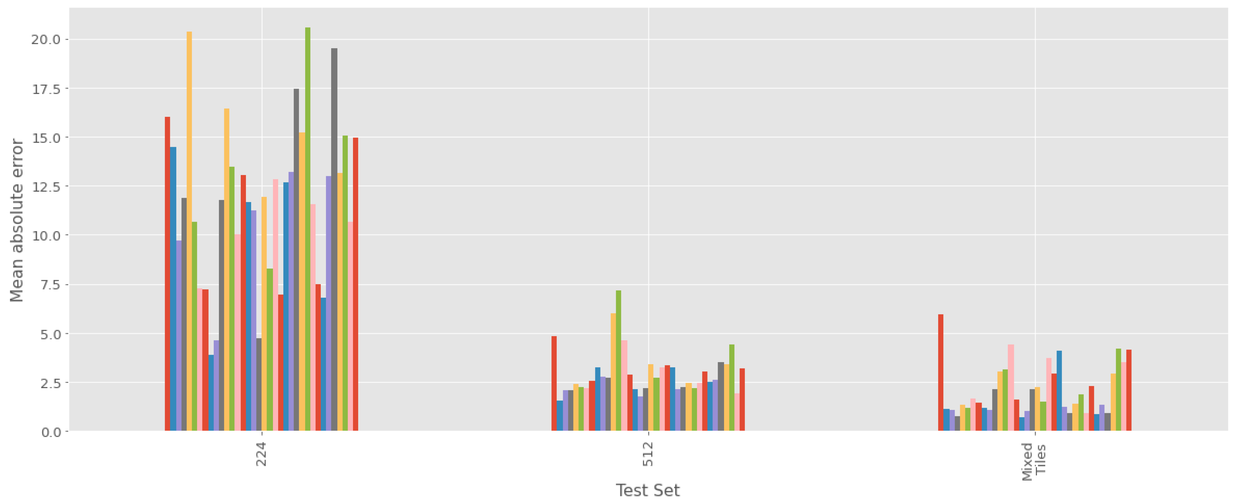
Figure 11.
Mean absolute error of three ResNet-50 models trained for 50 epochs with: 224 × 224-pixel tiles, 512 × 512-pixel tiles and a mix of both. Learning rate of 0.001 and a Batch Size of 32. Results displayed against a test set containing only 224 × 224-pixel tiles (orange), 512 × 512-pixel tiles (light blue), and a mix of both (dark blue).
Figure 12.
Mean absolute error of three models: ResNet-50, ResNet-101 and ResNet-152, trained for 50 epochs with a mix of 224 × 224- and 512 × 512-pixel tiles, with a learning rate of 0.001 and a Batch Size of 32. Results displayed against a test set containing only 224 × 224-pixel tiles (orange), 512 × 512-pixel tiles (light blue), and a mix of both (dark blue).
Figure 13.
Comparison of mean absolute error of all trained models in order against a test set composed of 224 × 224-pixel tiles, 512 × 512-pixel tiles and a mix of both. Each color represents a single ResNet model with specific hyperparameters.
Figure 13.
Comparison of mean absolute error of all trained models in order against a test set composed of 224 × 224-pixel tiles, 512 × 512-pixel tiles and a mix of both. Each color represents a single ResNet model with specific hyperparameters.
Figure 14.
Accuracy (MAE) of ResNet50 with different hyperparameters (batch size and learning rate) after 50 Epochs of training.
Figure 14.
Accuracy (MAE) of ResNet50 with different hyperparameters (batch size and learning rate) after 50 Epochs of training.
Figure 15.
Accuracy (MAE) of ResNet101 with different hyperparameters (batch size and learning rate) after 50 Epochs of training.
Figure 15.
Accuracy (MAE) of ResNet101 with different hyperparameters (batch size and learning rate) after 50 Epochs of training.
Figure 16.
Accuracy (MAE) of ResNet152 with different hyperparameters (batch size and learning rate) after 50 Epochs of training.
Figure 16.
Accuracy (MAE) of ResNet152 with different hyperparameters (batch size and learning rate) after 50 Epochs of training.
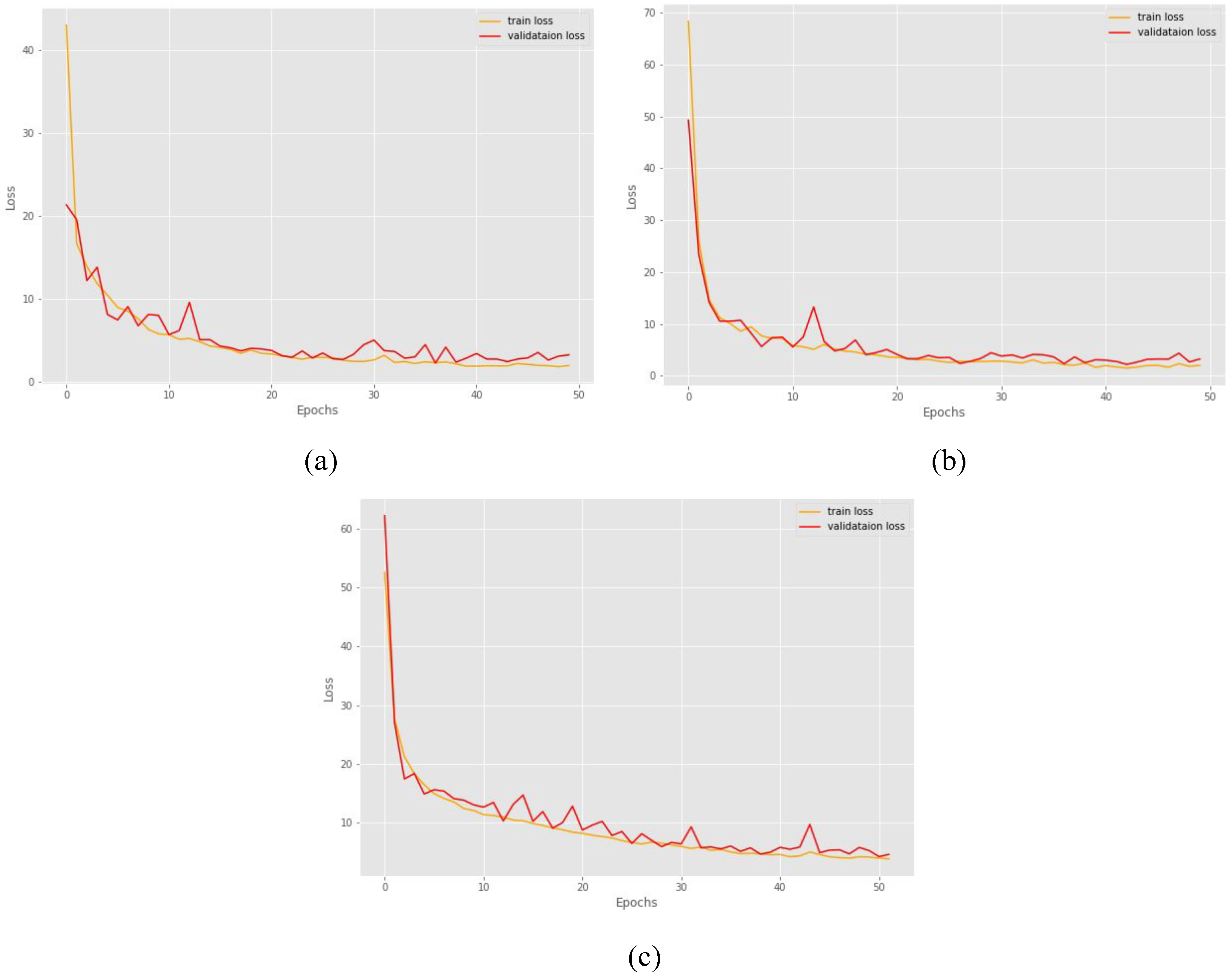
Figure 17.
Graphs comparing the training loss MAE (orange) and validation loss MAE (red) on different models across 50 epochs of training. (a) ResNet 50: learning rate = 0.01, batch size = 64, (b) ResNet 101: learning rate = 0.001, batch size = 96 and (c) ResNet 152: learning rate = 0.01, batch size = 16.
Figure 18.
Frequency distribution plot for the difference between the human-labeled and model-predicted point coordinates (X red and Y blue). Three architectures trained for 50 epochs are displayed: (a) ResNet 50: learning rate = 0.001, batch size = 32, (b) ResNet 101: learning rate = 0.0001, batch size = 64 and (c) ResNet 152: learning rate = 0.001, batch size = 32.
Figure 19.
Frequency distribution plot for the difference between the human-labeled and model-predicted point coordinates (X red and Y blue). Three architectures trained for 200 epochs are displayed: (a) ResNet-50: learning rate = 0.001, batch size = 32, (b) ResNet-101: learning rate = 0.0001, batch size = 64 and (c) ResNet-152: learning rate = 0.001, batch size = 32.
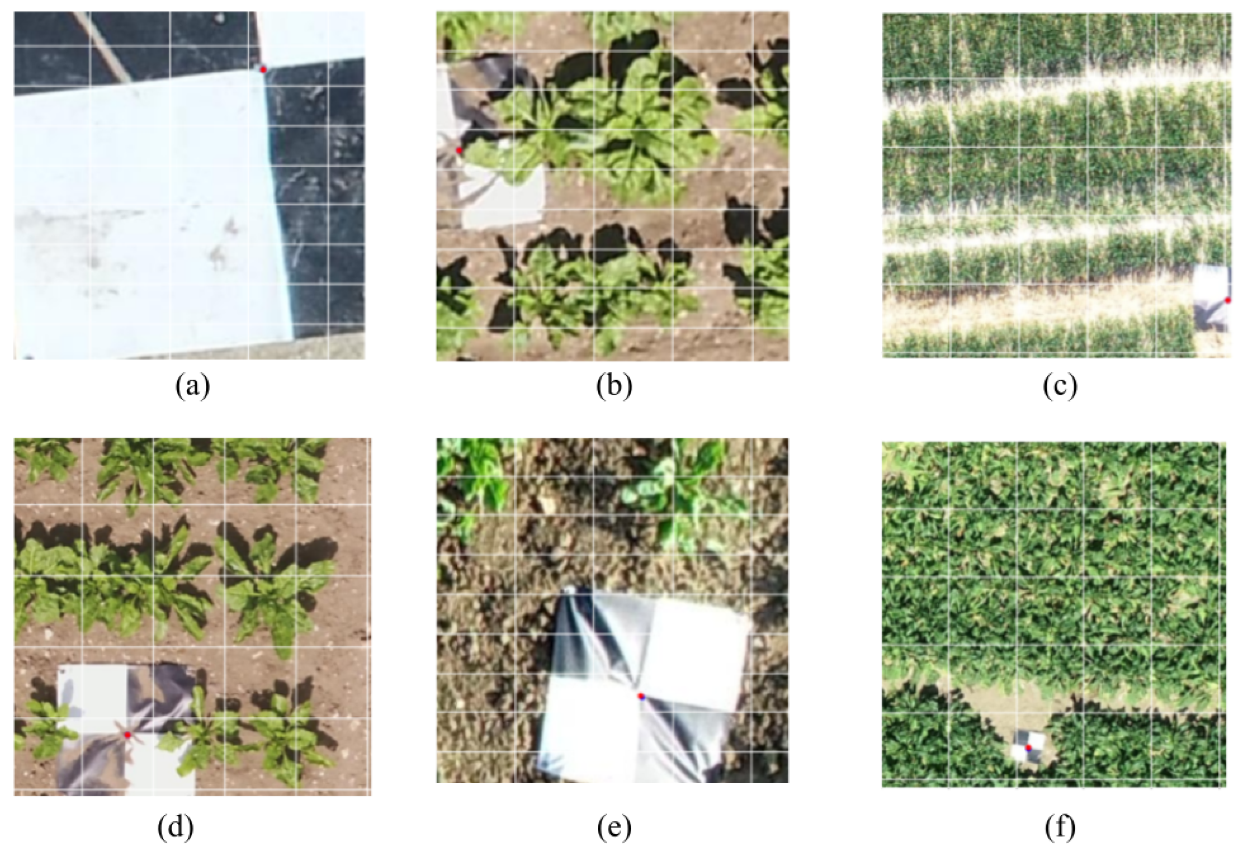
Figure 20.
Examples of the top 50% predictions of the ResNet-152 trained for 200 epochs with batch size = 32 and learning rate = 0.0001. The blue point represents the human-labeled keypoint and the red point represents the prediction.
Figure 20.
Examples of the top 50% predictions of the ResNet-152 trained for 200 epochs with batch size = 32 and learning rate = 0.0001. The blue point represents the human-labeled keypoint and the red point represents the prediction.
Figure 21.
Examples of the bottom 5% predictions of the ResNet-152 trained for 200 epochs with batch size = 32 and learning rate = 0.0001. The blue point represents the human-labeled center point and the red point represents the prediction.
Figure 21.
Examples of the bottom 5% predictions of the ResNet-152 trained for 200 epochs with batch size = 32 and learning rate = 0.0001. The blue point represents the human-labeled center point and the red point represents the prediction.
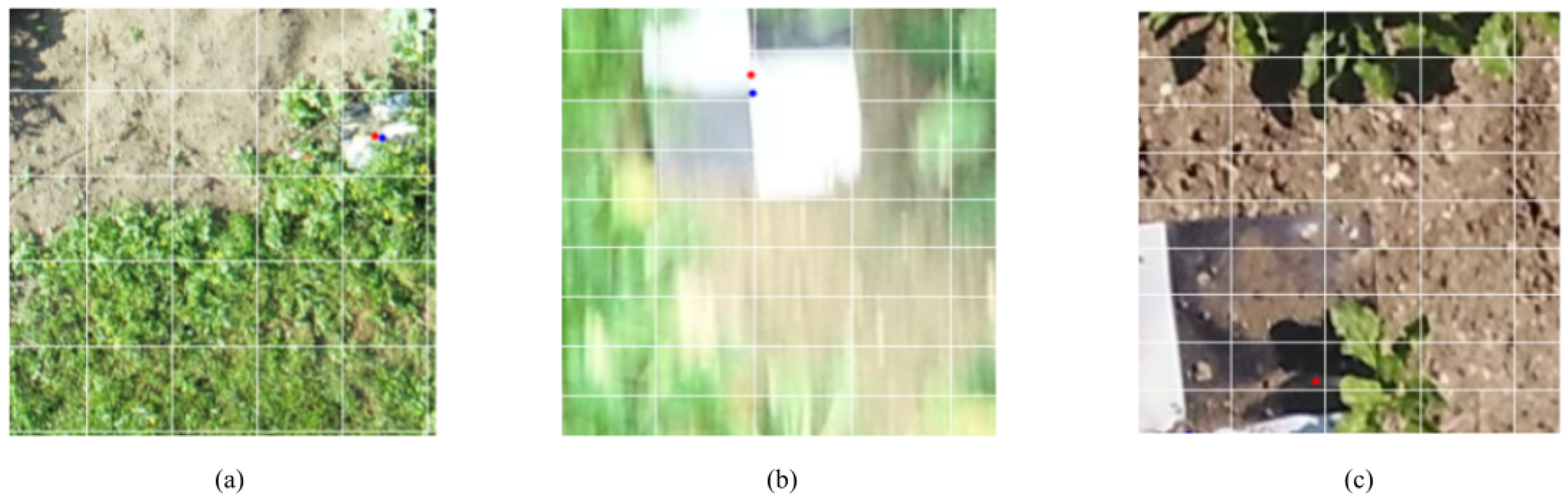
Figure 22.
Three prediction examples with human error by the ResNet152 batch size = 32, learning rate = 0.0001, the blue point represents the human-labeled center point and the red point represents the prediction. Images (a,c) are 512 × 512-pixel tiles, and (b) is 224 × 224-pixel tiles.
Figure 22.
Three prediction examples with human error by the ResNet152 batch size = 32, learning rate = 0.0001, the blue point represents the human-labeled center point and the red point represents the prediction. Images (a,c) are 512 × 512-pixel tiles, and (b) is 224 × 224-pixel tiles.
Figure 23.
Example of the classifier on a full size image. The blue tinted tiles are the ones classified as containing a GCP.
Figure 23.
Example of the classifier on a full size image. The blue tinted tiles are the ones classified as containing a GCP.
Table 1.
Maker, model, and number of pictures taken by each drone used in the study.
Table 1.
Maker, model, and number of pictures taken by each drone used in the study.
Maker
Pictures Taken | Model | Pictures Taken |
|---|
| DJI | FC550 | 120 |
| DJI | FC6310 | 1077 |
| DJI | FC6310R | 763 |
| DJI | FC6310S | 25 |
| DJI | FC6510 | 79 |
| DJI | FC6520 | 334 |
| DJI | FC6540 | 132 |
| DJI | M600_X5R | 28 |
| DJI | ZenmuseP1 | 299 |
| Hasselblad | L1D-20c | 24 |
| SONY | DSC-RX1RM2 | 76 |
Table 2.
Size and number of parameters for residual neural networks utilized.
Table 2.
Size and number of parameters for residual neural networks utilized.
| Model | Number of Parameters | Size of Model |
|---|
| ResNet-50 | 23,512,130 | 277.289 MB |
| ResNet-101 | 42,504,258 | 397.366 MB |
| ResNet-152 | 58,147,906 | 674.413 MB |
Table 3.
Errors on predictions of the test set of models trained with different loss functions.
Table 3.
Errors on predictions of the test set of models trained with different loss functions.
| Model Trained with | Mean Absolute Error | Mean Squared Error | Smooth L1 |
|---|
| MAE | 0.858 | 1.405 | 0.481 |
| MSE | 3.074 | 21.338 | 2.606 |
| SL1 | 1.237 | 2.788 | 0.831 |
Table 4.
Common hyperparameters utilized to train all models.
Table 4.
Common hyperparameters utilized to train all models.
| Hyperparameters | Value |
|---|
| Training epochs | 50 |
| Loss function | MAE |
| Training slip | ≈70% |
| Validation slip | ≈15% |
| Test slip | ≈15% |
| Transfer learning | ImageNet |
| Activation function | Linear |
| Optimizer | Adam |
Table 5.
Average mean absolute error across all trained models on different ResNet architectures with different test sets: 224 × 224-pixel tiles, 512 × 512-pixels tiles, and a mix of both.
Table 5.
Average mean absolute error across all trained models on different ResNet architectures with different test sets: 224 × 224-pixel tiles, 512 × 512-pixels tiles, and a mix of both.
| Architecture | MAE for 224 × 224 | MAE for 512 × 512 | MAE for Mix Tiles |
|---|
| ResNet50 | 13.732 | 2.775 | 2.038 |
| ResNet101 | 11.272 | 3.309 | 2.099 |
| ResNet152 | 10.365 | 2.771 | 2.215 |
Table 6.
Mean MAE and MSE as well as the standard deviation for the results of all trained models in all three architectures.
Table 6.
Mean MAE and MSE as well as the standard deviation for the results of all trained models in all three architectures.
| Architecture | Mean MAE | Standard Deviation for MAE | Mean MSE | Standard Deviation for MSE |
|---|
| ResNet50 | 2.133 | 1.265 | 12.061 | 12.915 |
| ResNet101 | 1.841 | 1.116 | 9.180 | 10.439 |
| ResNet152 | 2.215 | 1.172 | 14.032 | 14.473 |
Table 7.
Mean MAE and MSE as well as the standard deviation for the results of all trained models in all three studied learning rates.
Table 7.
Mean MAE and MSE as well as the standard deviation for the results of all trained models in all three studied learning rates.
| Learning Rate | Mean MAE | Standard Deviation for MAE | Mean MSE | Standard Deviation for MSE |
|---|
| 0.01 | 3.475 | 0.716 | 26.328 | 9.477 |
| 0.001 | 1.505 | 0.516 | 5.860 | 4.998 |
| 0.0001 | 1.167 | 0.341 | 2.463 | 1.437 |
Table 8.
Mean MAE and MSE as well as the standard deviation for the results of all trained models in all three studied batch sizes.
Table 8.
Mean MAE and MSE as well as the standard deviation for the results of all trained models in all three studied batch sizes.
| Batch Size | Mean MAE | Standard Deviation for MAE | Mean MSE | Standard Deviation for MSE |
|---|
| 16 | 2.083 | 0.831 | 12.877 | 11.618 |
| 32 | 1.929 | 1.228 | 10.446 | 12.340 |
| 64 | 1.995 | 1.244 | 10.752 | 12.975 |
| 96 | 2.260 | 1.596 | 12.415 | 15.187 |
Table 9.
Comparison of the MAE for the top three performing models after being trained for 50 and 200 epochs. (ResNet-50: learning rate = 0.001, batch size = 32, ResNet-101: learning rate = 0.0001, batch size = 64 and ResNet-152: learning rate = 0.0001, batch size = 32.)
Table 9.
Comparison of the MAE for the top three performing models after being trained for 50 and 200 epochs. (ResNet-50: learning rate = 0.001, batch size = 32, ResNet-101: learning rate = 0.0001, batch size = 64 and ResNet-152: learning rate = 0.0001, batch size = 32.)
| Architecture | MAE after 50 Epochs | MAE after 200 Epochs |
|---|
| ResNet-50 | 0.858 | 0.664 |
| ResNet-101 | 0.746 | 0.632 |
| ResNet-152 | 0.721 | 0.586 |
Table 10.
Average training time for 50 epochs for all tester architectures.
Table 10.
Average training time for 50 epochs for all tester architectures.
| Architecture | Average Training Time (s) | Average Training Time (HH:MM:SS) | Average Seconds per Epoch |
|---|
| ResNet-50 | 6559.116 | 01:49:19 | 131.182 |
| ResNet-101 | 9802.033 | 02:43:22 | 196.040 |
| ResNet-152 | 11,893.568 | 03:18:13 | 237.871 |
Table 11.
Average time of prediction of 1200 tiles with batch size = 32 for different architectures with only a CPU and with the use of a GPU.
Table 11.
Average time of prediction of 1200 tiles with batch size = 32 for different architectures with only a CPU and with the use of a GPU.
| Architecture | Average Seconds CPU | Average Min:Sec CPU | Average Seconds GPU | Average Min:Sec GPU |
|---|
| ResNet50 | 238.083 | 03:58 | 6.687 | 00:07 |
| ResNet101 | 401.205 | 06:41 | 7.482 | 00:07 |
| ResNet152 | 582.306 | 09:42 | 9.415 | 00:09 |
Table 12.
Results of the Lobe trained classifier.
Table 12.
Results of the Lobe trained classifier.
| Statistic | Percentage |
|---|
| GCP classified as GCP | 96.8034% |
| GCP classified as Empty | 3.1965% |
| Empty classified as Empty | 96.5290% |
| Empty classified as GCP | 3.4709% |
| Total Accuracy | 96.6847% |


