
Synthesizing Local Capacities, Multi-Source Remote Sensing and Meta-Learning to Optimize Forest Carbon Assessment in Data-Poor Regions

 , , , ,
Abstract
1. Introduction
2. Materials and Methods
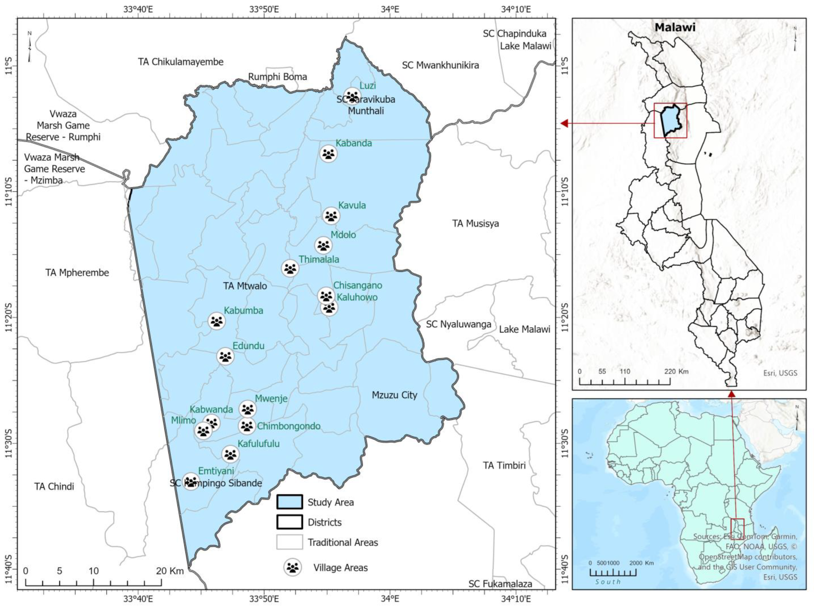
2.1. Study Area
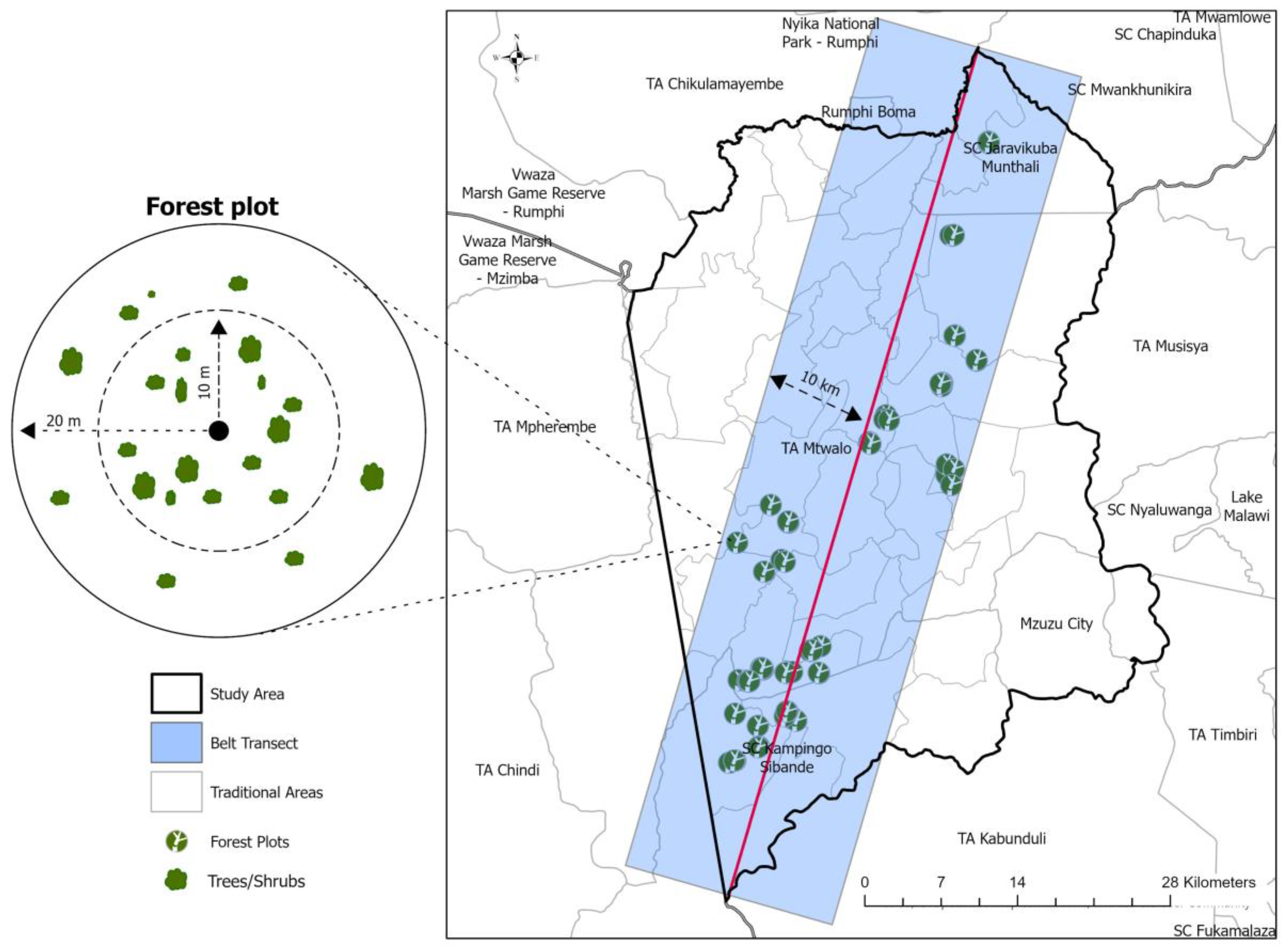
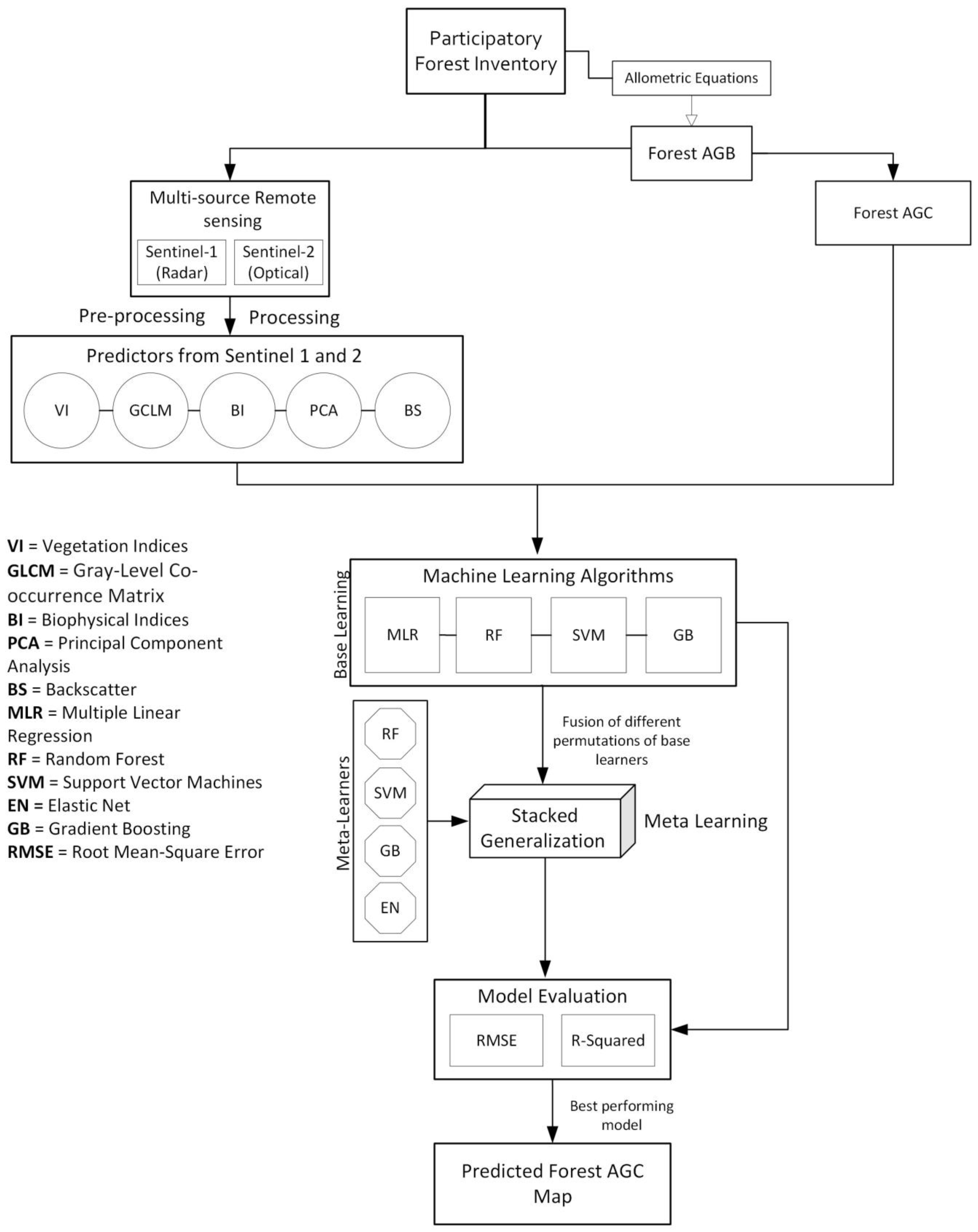
2.2. Study Design
Participatory Forest Inventory
2.3. Data Collection and Processing
2.3.1. Plot Demarcation and Assessment
2.3.2. Tree Measurements
2.4. Analysis
2.4.1. Ecological Indices
2.4.2. Forest Above Ground Biomass Using Allometric Equations
2.4.3. Optical and Radar Remote Sensing
2.4.4. Base Machine Learners
Multiple Linear Regression (MLR)
Random Forest (RF)
Support Vector Machine (SVM)
Gradient Boosting (GB)
2.4.5. Meta-Learning Using Stacked Generalization Ensemble
2.4.6. Evaluation of Base and Meta Models
3. Results
3.1. Participatory Forest Inventory: Ecological Insights and Management Practices
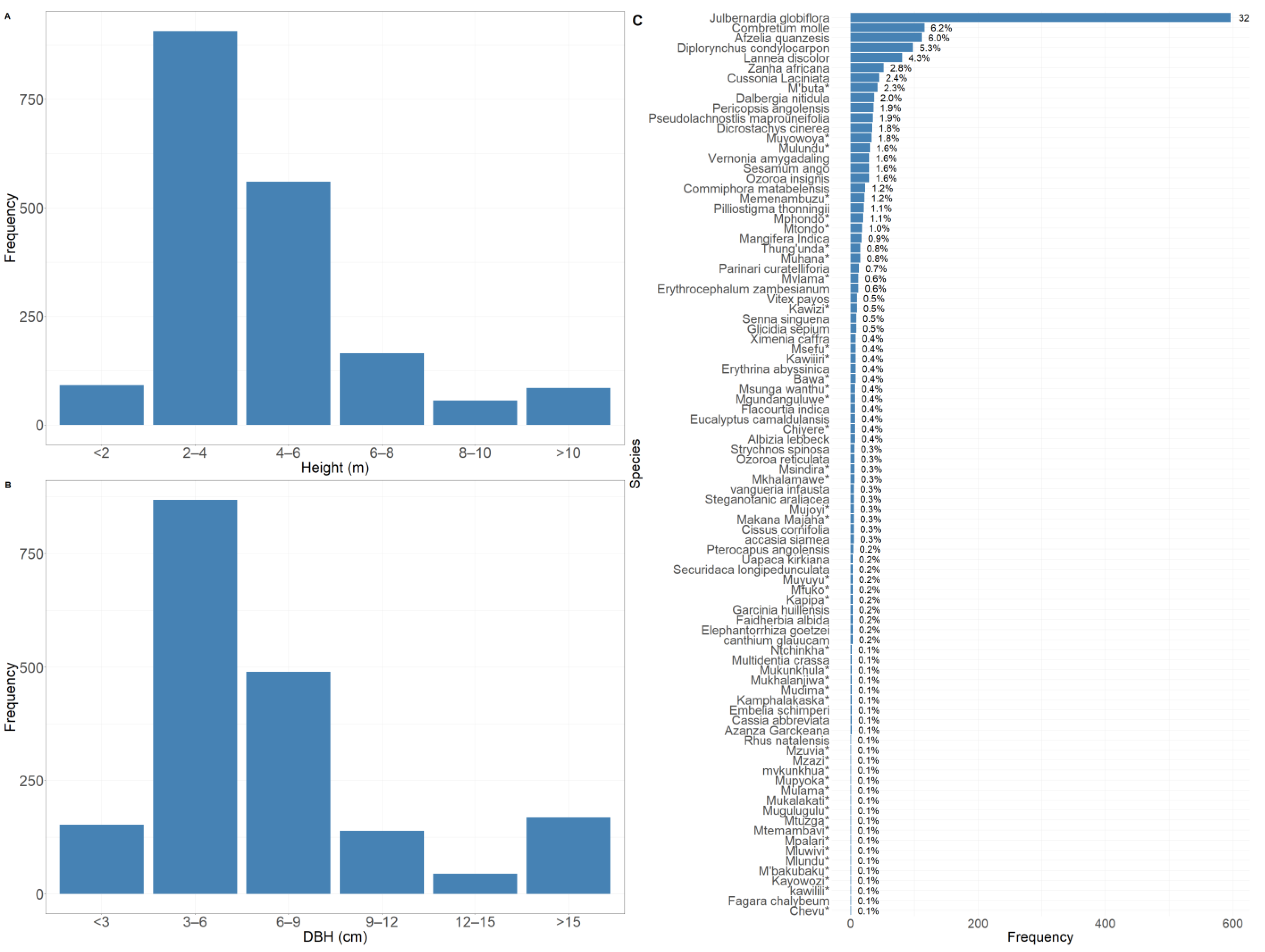
3.1.1. Tree Species, Diameter, and Height
3.1.2. Forest Stand Density and Species Diversity
3.2. Evaluation of Allometric Equations for Estimating Forest AGB
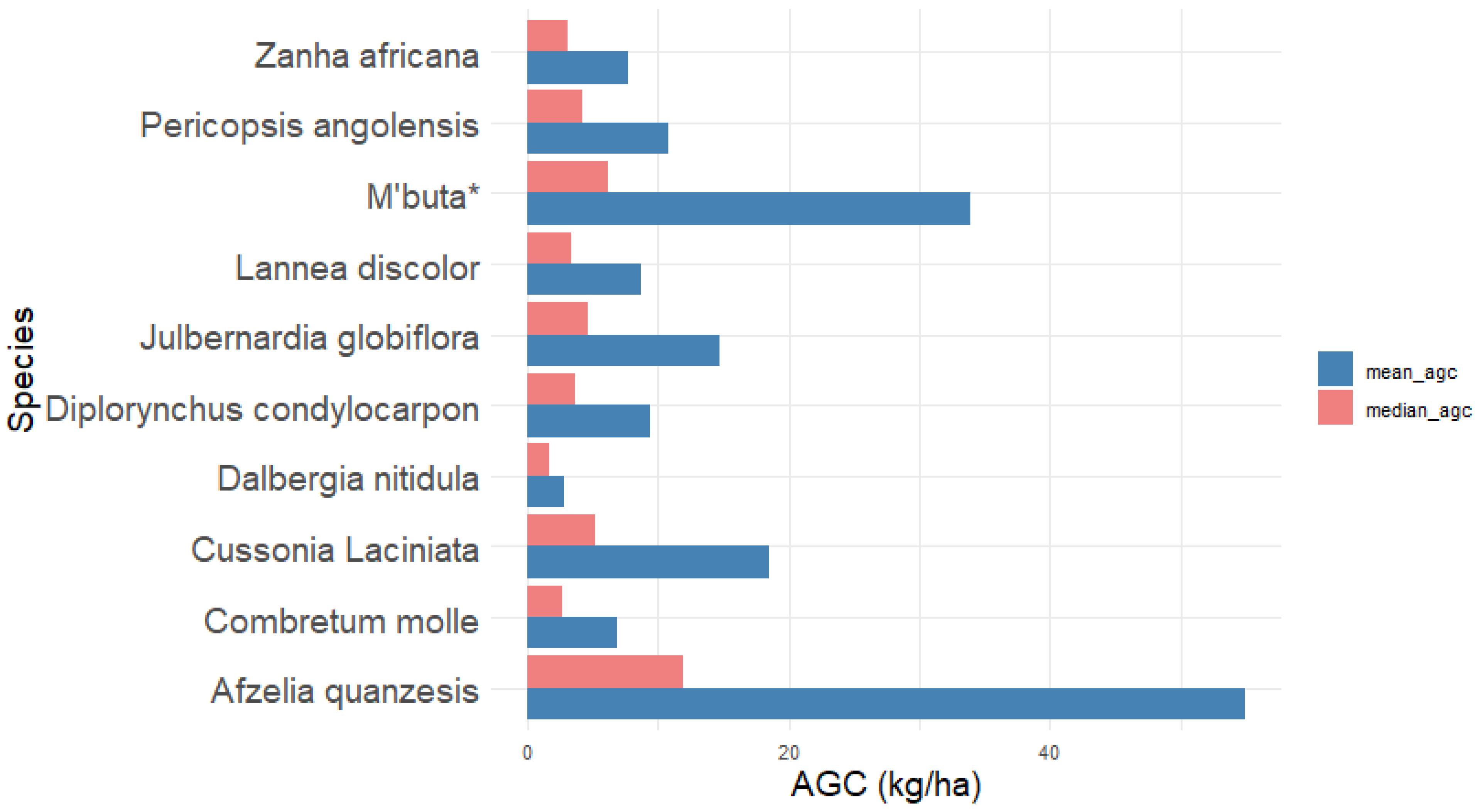
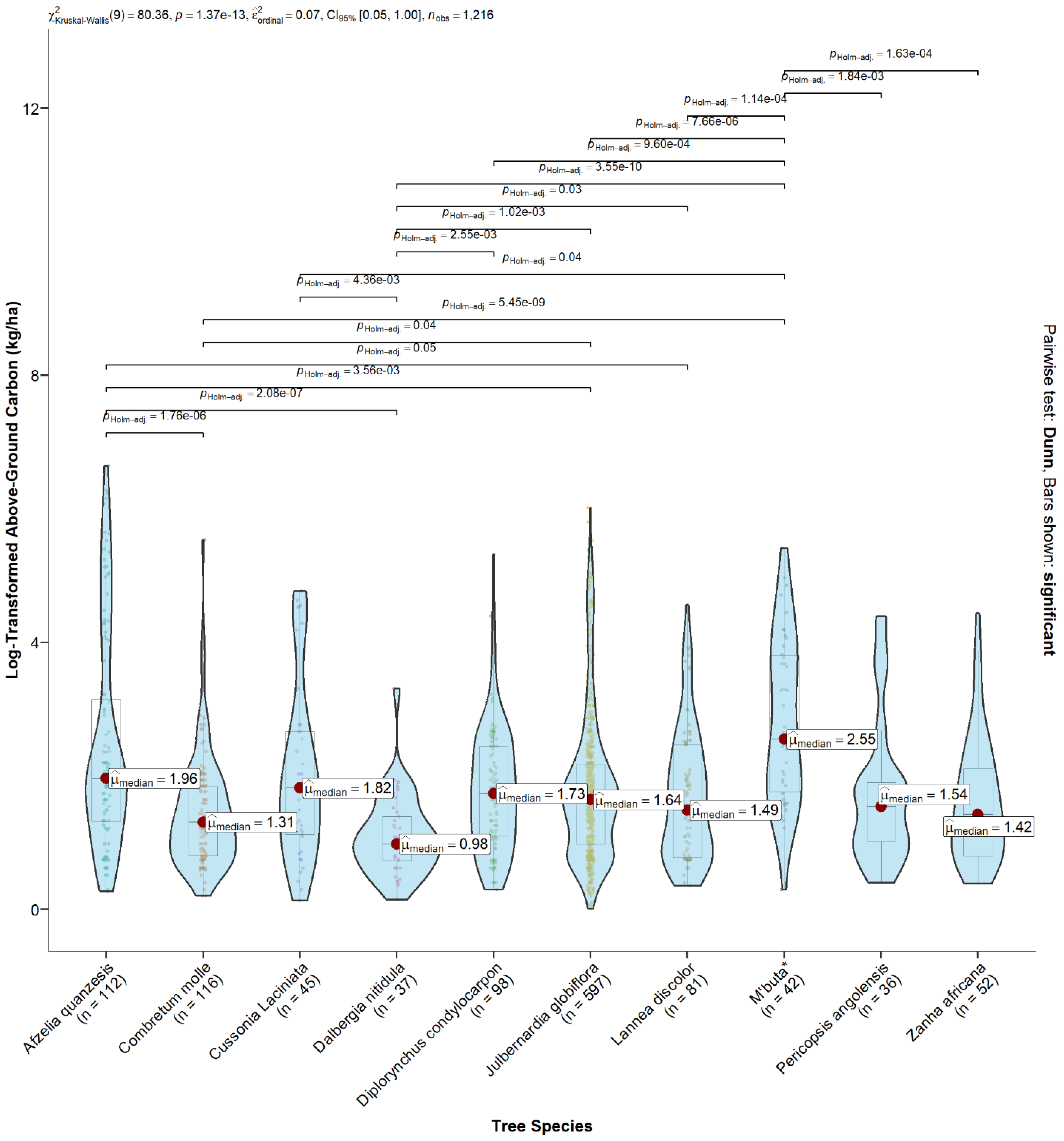
3.3. Forest Species and Carbon Stocks
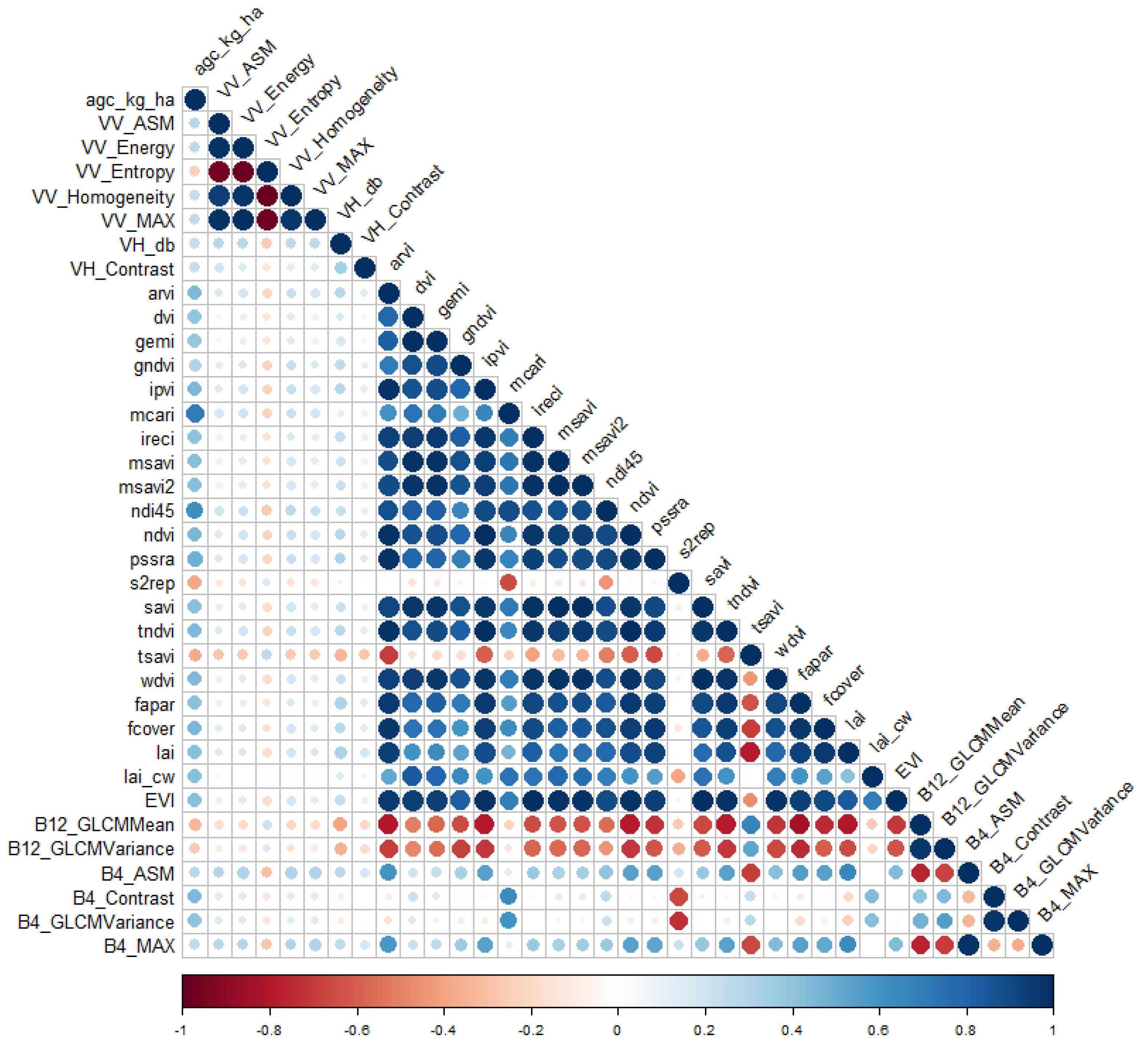
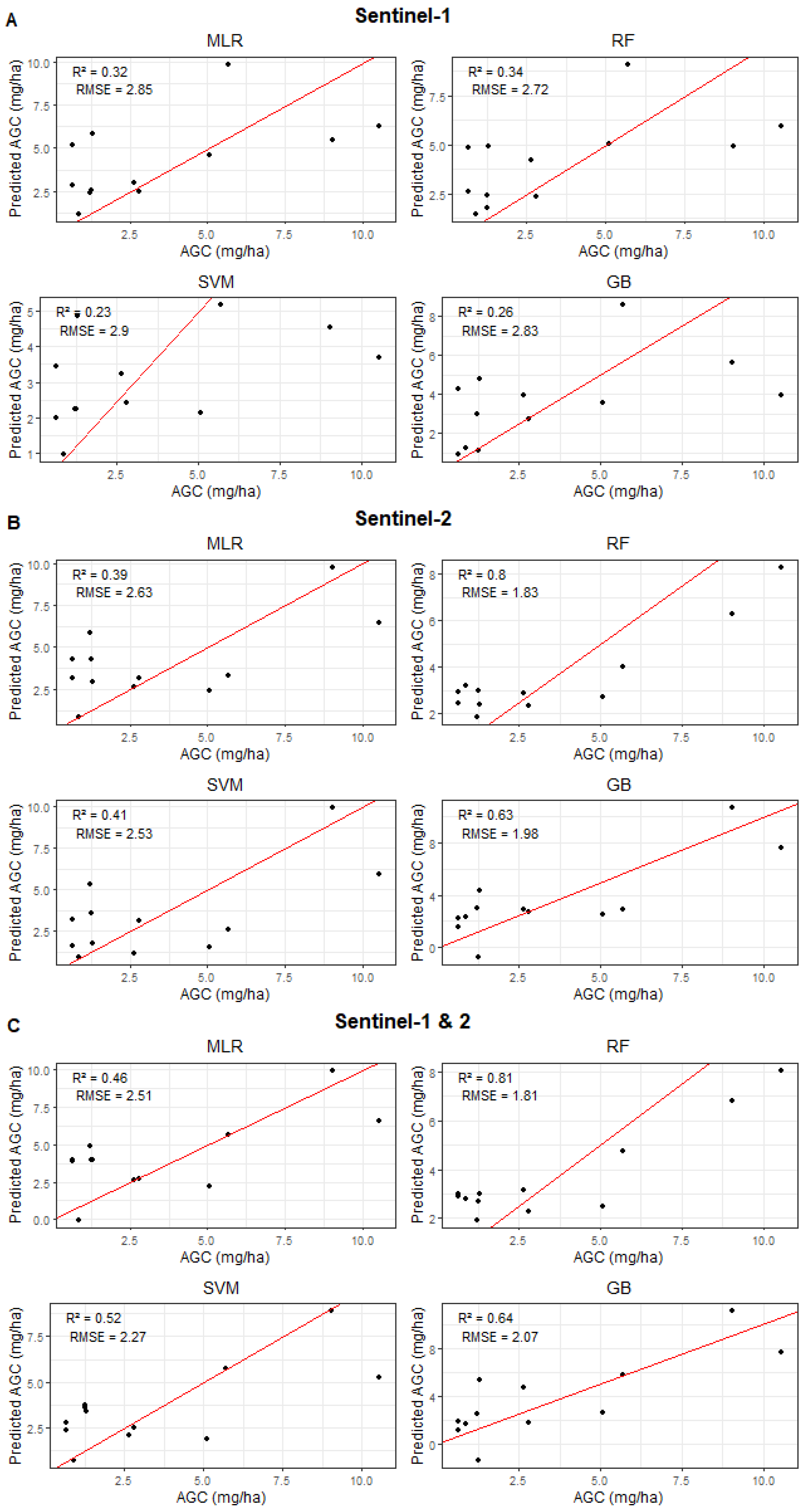
3.4. AGC Prediction Using Multi-Source Remote Sensing and Machine Learning
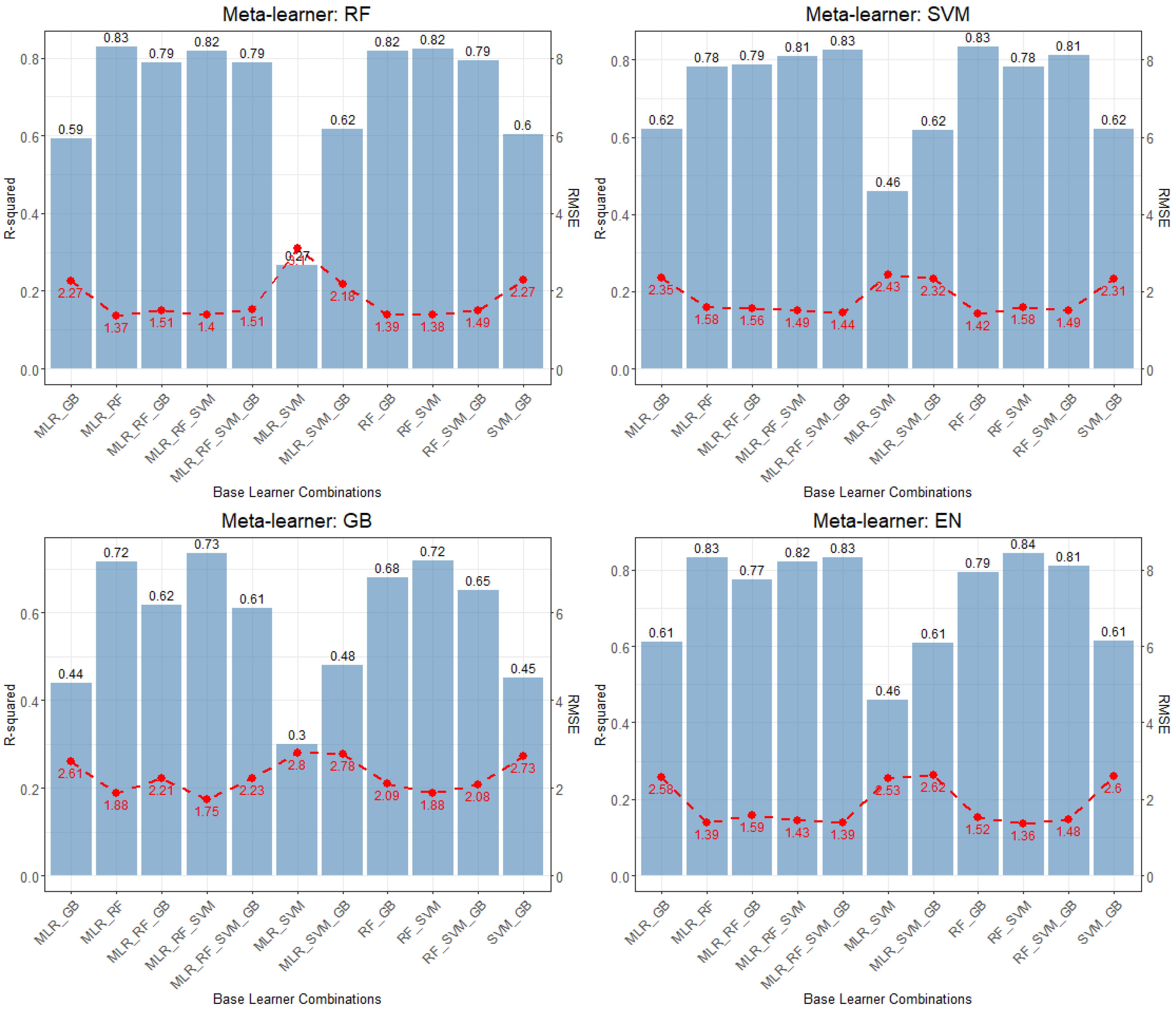
3.5. Forest AGC Prediction Stacked Generalization
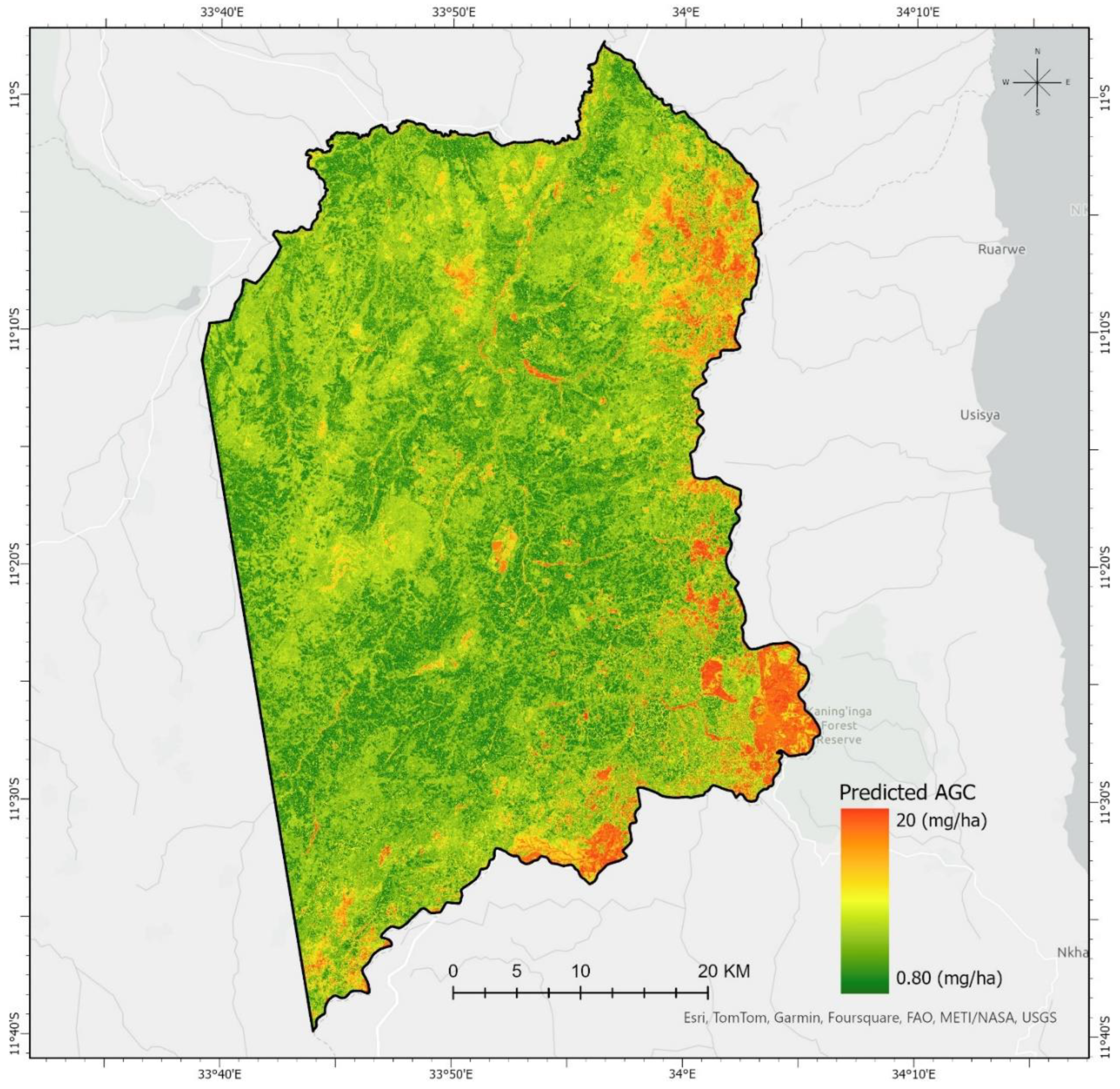
3.6. Spatial Distribution of Forest AGC
4. Discussion
4.1. Participatory Inventories and Local Knowledge in Assessing Tree Species’ Carbon Stocks
4.2. Integrating Optical and Radar Remote Sensing for Improved Forest AGC Prediction
4.3. Advancing Forest AGC Prediction Through Stacking: Examining Learner Diversity and Model Sensitivity
5. Conclusions
Author Contributions
Funding
Data Availability Statement
Conflicts of Interest
References
- Anyona, S.; Rop, B. Mitigating Against Conflicts in the Kenyan Mining Cycle: Identification of Gaps in the Participation and Recourse for Rights Holders (Civil Society & Community). E3S Web Conf. 2017, 15, 02005. [Google Scholar]
- Fawzy, S.; Osman, A.I.; Doran, J.; Rooney, D.W. Strategies for Mitigation of Climate Change: A Review. Environ. Chem. Lett. 2020, 18, 2069–2094. [Google Scholar] [CrossRef]
- Kauppi, P.E.; Stål, G.; Arnesson-Ceder, L.; Hallberg Sramek, I.; Hoen, H.F.; Svensson, A.; Wernick, I.K.; Högberg, P.; Lundmark, T.; Nordin, A. Managing Existing Forests Can Mitigate Climate Change. For. Ecol. Manag. 2022, 513, 120186. [Google Scholar] [CrossRef]
- Hagedorn, F.; Landolt, W.; Tarjan, D.; Egli, P.; Bucher, J.B. Elevated CO2 Influences Nutrient Availability in Young Beech-Spruce Communities on Two Soil Types. Oecologia 2002, 132, 109–117. [Google Scholar] [CrossRef] [PubMed]
- Keenan, T.F.; Williams, C.A. The Terrestrial Carbon Sink. Annu. Rev. Environ. Resour. 2018, 43, 219–243. [Google Scholar] [CrossRef]
- Tang, K.; Zhao, X.; Xu, Z.; Sun, H. A Stacking Ensemble Model for Predicting Soil Organic Carbon Content Based on Visible and Near-Infrared Spectroscopy. Infrared Phys. Technol. 2024, 140, 105404. [Google Scholar] [CrossRef]
- Alonzo, M.; Bookhagen, B.; Roberts, D.A. Urban Tree Species Mapping Using Hyperspectral and Lidar Data Fusion. Remote Sens. Environ. 2014, 148, 70–83. [Google Scholar] [CrossRef]
- Cao, L.; Coops, N.C.; Sun, Y.; Ruan, H.; Wang, G.; Dai, J.; She, G. Estimating Canopy Structure and Biomass in Bamboo Forests Using Airborne LiDAR Data. ISPRS J. Photogramm. Remote Sens. 2019, 148, 114–129. [Google Scholar] [CrossRef]
- Patenaude, G.; Hill, R.A.; Milne, R.; Gaveau, D.L.A.; Briggs, B.B.J.; Dawson, T.P. Quantifying Forest above Ground Carbon Content Using LiDAR Remote Sensing. Remote Sens. Environ. 2004, 93, 368–380. [Google Scholar] [CrossRef]
- Danielsen, F.; Jensen, P.M.; Burgess, N.D.; Altamirano, R.; Alviola, P.A.; Andrianandrasana, H.; Brashares, J.S.; Burton, A.C.; Coronado, I.; Corpuz, N.; et al. A Multicountry Assessment of Tropical Resource Monitoring by Local Communities. BioScience 2014, 64, 236–251. [Google Scholar] [CrossRef]
- Mateo-Vega, J.; Potvin, C.; Monteza, J.; Bacorizo, J.; Barrigón, J.; Barrigón, R.; López, N.; Omi, L.; Opua, M.; Serrano, J.; et al. Full and Effective Participation of Indigenous Peoples in Forest Monitoring for Reducing Emissions from Deforestation and Forest Degradation (REDD+): Trial in Panama’s Darién. Ecosphere 2017, 8, e01635. [Google Scholar] [CrossRef]
- de Vos, A.; Preiser, R.; Masterson, V.A. Participatory Data Collection. In The Routledge Handbook of Research Methods for Social-ecological Systems; Routledge: London, UK, 2021; p. 119. [Google Scholar]
- Kpienbaareh, D.; Mohammed, K.; Luginaah, I.; Wang, J.; Bezner Kerr, R.; Lupafya, E.; Dakishoni, L. Local Actors, Farmer Decisions and Landscape Crop Diversity in Smallholder Farming Systems: A Systems Perspective. Agric. Ecosyst. Environ. 2024, 374, 109138. [Google Scholar] [CrossRef]
- Mukama, K.; Mustalahti, I.; Zahabu, E. Participatory Forest Carbon Assessment and REDD+: Learning from Tanzania. Int. J. For. Res. 2012, 2012, 126454. [Google Scholar] [CrossRef]
- Dos Reis, A.A.; Werner, J.P.S.; Silva, B.C.; Figueiredo, G.K.D.A.; Antunes, J.F.G.; Esquerdo, J.C.D.M.; Coutinho, A.C.; Lamparelli, R.A.C.; Rocha, J.V.; Magalhães, P.S.G. Monitoring Pasture Aboveground Biomass and Canopy Height in an Integrated Crop–Livestock System Using Textural Information from PlanetScope Imagery. Remote Sens. 2020, 12, 2534. [Google Scholar] [CrossRef]
- Mohajane, M.; Costache, R.; Karimi, F.; Bao Pham, Q.; Essahlaoui, A.; Nguyen, H.; Laneve, G.; Oudija, F. Application of Remote Sensing and Machine Learning Algorithms for Forest Fire Mapping in a Mediterranean Area. Ecol. Indic. 2021, 129, 107869. [Google Scholar] [CrossRef]
- Zhang, F.; Tian, X.; Zhang, H.; Jiang, M. Estimation of Aboveground Carbon Density of Forests Using Deep Learning and Multisource Remote Sensing. Remote Sens. 2022, 14, 3022. [Google Scholar] [CrossRef]
- Anees, S.A.; Mehmood, K.; Khan, W.R.; Sajjad, M.; Alahmadi, T.A.; Alharbi, S.A.; Luo, M. Integration of Machine Learning and Remote Sensing for above Ground Biomass Estimation through Landsat-9 and Field Data in Temperate Forests of the Himalayan Region. Ecol. Inform. 2024, 82, 102732. [Google Scholar] [CrossRef]
- Aziz, G.; Minallah, N.; Saeed, A.; Frnda, J.; Khan, W. Remote Sensing Based Forest Cover Classification Using Machine Learning. Sci. Rep. 2024, 14, 69. [Google Scholar] [CrossRef]
- Haque, M.A.; Reza, M.N.; Ali, M.; Karim, M.R.; Ahmed, S.; Lee, K.-D.; Khang, Y.H.; Chung, S.-O. Effects of Environmental Conditions on Vegetation Indices from Multispectral Images: A Review. Korean J. Remote Sens. 2024, 40, 319–341. [Google Scholar] [CrossRef]
- Tian, L.; Wu, X.; Tao, Y.; Li, M.; Qian, C.; Liao, L.; Fu, W. Review of Remote Sensing-Based Methods for Forest Aboveground Biomass Estimation: Progress, Challenges, and Prospects. Forests 2023, 14, 1086. [Google Scholar] [CrossRef]
- Ali, N.; Khati, U. Forest Aboveground Biomass and Forest Height Estimation Over a Sub-Tropical Forest Using Machine Learning Algorithm and Synthetic Aperture Radar Data. J. Indian Soc. Remote Sens. 2024, 52, 771–786. [Google Scholar] [CrossRef]
- El Masri, B.; Xiao, J. Comparison of Global Aboveground Biomass Estimates From Satellite Observations and Dynamic Global Vegetation Models. J. Geophys. Res. Biogeosci. 2025, 130, e2024JG008305. [Google Scholar] [CrossRef]
- Le, A. Estimating Tropical Forest Above-Ground Biomass at the Local Scale Using Multi-Source Space-Borne Remote Sensing Data. PhD Thesis, UNSW Sydney, Sydney, NSW, Australia, 2023. [Google Scholar]
- Rana, P.; Popescu, S.; Tolvanen, A.; Gautam, B.; Srinivasan, S.; Tokola, T. Estimation of Tropical Forest Aboveground Biomass in Nepal Using Multiple Remotely Sensed Data and Deep Learning. Int. J. Remote Sens. 2023, 44, 5147–5171. [Google Scholar] [CrossRef]
- Government of Malawi. The Malawi Growth and Development Strategy (MGDS) III: Building a Productive, Competitive and Resilient Nation; Government of Malawi: Lilongwe, Malawi, 2017. [Google Scholar]
- Malawi Statistical Office. Main Report; Malawi Statistical Office: Zomba, Malawi, 2018; Volume 8. [Google Scholar]
- World Bank. Climate Change Knowledge Portal: Malawi; World Bank: Washington, DC, USA, 2020. [Google Scholar]
- Kuyah, S.; Sileshi, G.W.; Njoloma, J.; Mng’omba, S.; Neufeldt, H. Estimating Aboveground Tree Biomass in Three Different Miombo Woodlands and Associated Land Use Systems in Malawi. Biomass Bioenergy 2014, 66, 214–222. [Google Scholar] [CrossRef]
- Gondwe, M.F.K.; Geldenhuys, C.J.; Chirwa, P.W.C.; Assédé, E.S.P.; Syampungani, S.; Cho, M.A. Tree Species Composition and Diversity in Miombo Woodlands between Co-Managed and Government-Managed Regimes, Malawi. Afr. J. Ecol. 2021, 59, 225–240. [Google Scholar] [CrossRef]
- Mwase, W.F.; Bjørnstad, Å.; Bokosi, J.M.; Kwapata, M.B.; Stedje, B. The Role of Land Tenure in Conservation of Tree and Shrub Species Diversity in Miombo Woodlands of Southern Malawi. New For. 2007, 33, 297–307. [Google Scholar] [CrossRef]
- FAO. The State of Food and Agriculture 2015 (SOFA): Social Protection and Agriculture: Breaking the Cycle of Rural Poverty; FAO: Rome, Italy, 2015. [Google Scholar]
- Global Forest Watch Mzimba, Malawi Deforestation Rates & Statistics | GFW. Available online: https://www.globalforestwatch.org/dashboards/country/MWI/17/ (accessed on 31 October 2022).
- Pascual, C.; Mauro, F.; Hernando, A.; Martín-Fernández, S. Inventory Techniques in Participatory Forest Management. In Quantitative Techniques in Participatory Forest Management; CRC Press: Boca Raton, FL, USA, 2013; ISBN 978-0-429-08886-5. [Google Scholar]
- Yang, H.; Magnussen, S.; Fehrmann, L.; Mundhenk, P.; Kleinn, C. Two Neighborhood-Free Plot Designs for Adaptive Sampling of Forests. Environ. Ecol. Stat. 2016, 23, 279–299. [Google Scholar] [CrossRef]
- Marchant, B.P.; Lark, R.M. Adaptive Sampling and Reconnaissance Surveys for Geostatistical Mapping of the Soil. Eur. J. Soil Sci. 2006, 57, 831–845. [Google Scholar] [CrossRef]
- Rousselle, F.; Knaus, C.; Zwicker, M. Adaptive Sampling and Reconstruction Using Greedy Error Minimization. ACM Trans. Graph. 2011, 30, 1–12. [Google Scholar] [CrossRef]
- Thien, S.J. A Flow Diagram for Teaching Texture-by-Feel Analysis. J. Agron. Educ. 1979, 8, 54–55. [Google Scholar] [CrossRef]
- Brokaw, N.; Thompson, J. The h for Dbh. For. Ecol. Manag. 2000, 129, 89–91. [Google Scholar] [CrossRef]
- Shannon, C.E. A Mathematical Theory of Communication. Bell Syst. Tech. J. 1948, 27, 379–423. [Google Scholar] [CrossRef]
- Kachamba, D.J.; Eid, T.; Gobakken, T. Above-and Belowground Biomass Models for Trees in the Miombo Woodlands of Malawi. Forests 2016, 7, 38. [Google Scholar] [CrossRef]
- Kuyah, S.; Sileshi, G.W.; Rosenstock, T.S. Allometric Models Based on Bayesian Frameworks Give Better Estimates of Aboveground Biomass in the Miombo Woodlands. Forests 2016, 7, 13. [Google Scholar] [CrossRef]
- Malakini, M.; Makungwa, S.; Mwase, W.; Maganga, A.M. Allometric Models for Estimating Above- and below- Ground Tree Carbon for Community Managed Miombo Woodlands: A Case of Miyobe Village Forest Area in Northern Malawi. Trees For. People 2020, 2, 100024. [Google Scholar] [CrossRef]
- Chidumayo, E.N. Forest Degradation and Recovery in a Miombo Woodland Landscape in Zambia: 22 Years of Observations on Permanent Sample Plots. For. Ecol. Manag. 2013, 291, 154–161. [Google Scholar] [CrossRef]
- Kuyah, S.; Dietz, J.; Muthuri, C.; Jamnadass, R.; Mwangi, P.; Coe, R.; Neufeldt, H. Allometric Equations for Estimating Biomass in Agricultural Landscapes: I. Aboveground Biomass. Agric. Ecosyst. Environ. 2012, 158, 216–224. [Google Scholar] [CrossRef]
- Malimbwi, R.E.; Solberg, B.; Luoga, E. Estimation of Biomass and Volume in Miombo Woodland at Kitulangalo Forest Reserve, Tanzania. J. Trop. For. Sci. 1994, 7, 230–242. [Google Scholar]
- Mugasha, W.A.; Eid, T.; Bollandsås, O.M.; Malimbwi, R.E.; Chamshama, S.A.O.; Zahabu, E.; Katani, J.Z. Allometric Models for Prediction of Above- and Belowground Biomass of Trees in the Miombo Woodlands of Tanzania. For. Ecol. Manag. 2013, 310, 87–101. [Google Scholar] [CrossRef]
- Brown, S. Estimating Biomass and Biomass Change of Tropical Forests: A Primer; FAO: Rome, Italy, 1997; Volume 134. [Google Scholar]
- Chave, J.; Réjou-Méchain, M.; Búrquez, A.; Chidumayo, E.; Colgan, M.S.; Delitti, W.B.C.; Duque, A.; Eid, T.; Fearnside, P.M.; Goodman, R.C.; et al. Improved Allometric Models to Estimate the Aboveground Biomass of Tropical Trees. Glob. Change Biol. 2014, 20, 3177–3190. [Google Scholar] [CrossRef]
- Ma, S.; He, F.; Tian, D.; Zou, D.; Yan, Z.; Yang, Y.; Zhou, T.; Huang, K.; Shen, H.; Fang, J. Variations and Determinants of Carbon Content in Plants: A Global Synthesis. Biogeosciences 2018, 15, 693–702. [Google Scholar] [CrossRef]
- Martin, A.R.; Thomas, S.C. A Reassessment of Carbon Content in Tropical Trees. PLoS ONE 2011, 6, e23533. [Google Scholar] [CrossRef] [PubMed]
- Weggler, K.; Dobbertin, M.; Jüngling, E.; Kaufmann, E.; Thürig, E. Dead Wood Volume to Dead Wood Carbon: The Issue of Conversion Factors. Eur. J. For. Res. 2012, 131, 1423–1438. [Google Scholar] [CrossRef]
- Venkatappa, M.; Sasaki, N.; Anantsuksomsri, S.; Smith, B. Applications of the Google Earth Engine and Phenology-Based Threshold Classification Method for Mapping Forest Cover and Carbon Stock Changes in Siem Reap Province, Cambodia. Remote Sens. 2020, 12, 3110. [Google Scholar] [CrossRef]
- Vicharnakorn, P.; Shrestha, R.P.; Nagai, M.; Salam, A.P.; Kiratiprayoon, S. Carbon Stock Assessment Using Remote Sensing and Forest Inventory Data in Savannakhet, Lao PDR. Remote Sens. 2014, 6, 5452–5479. [Google Scholar] [CrossRef]
- Waldeland, A.U.; Trier, Ø.D.; Salberg, A.-B. Forest Mapping and Monitoring in Africa Using Sentinel-2 Data and Deep Learning. Int. J. Appl. Earth Obs. Geoinf. 2022, 111, 102840. [Google Scholar] [CrossRef]
- Wang, C.; Zhang, W.; Ji, Y.; Marino, A.; Li, C.; Wang, L.; Zhao, H.; Wang, M. Estimation of Aboveground Biomass for Different Forest Types Using Data from Sentinel-1, Sentinel-2, ALOS PALSAR-2, and GEDI. Forests 2024, 15, 215. [Google Scholar] [CrossRef]
- Breiman, L. Random Forests. Mach. Learn. 2001, 45, 5–32. [Google Scholar] [CrossRef]
- Cai, J.; Xu, K.; Zhu, Y.; Hu, F.; Li, L. Prediction and Analysis of Net Ecosystem Carbon Exchange Based on Gradient Boosting Regression and Random Forest. Appl. Energy 2020, 262, 114566. [Google Scholar] [CrossRef]
- Jensen, J.R. Introductory Digital Image Processing: A Remote Sensing Perspective, 4th ed.; Pearson series in geographic information science; Pearson Education Inc.: Glenview, IL, USA, 2016; ISBN 978-0-13-405816-0. [Google Scholar]
- Awad, M.; Khanna, R. Support Vector Regression. In Efficient Learning Machines: Theories, Concepts, and Applications for Engineers and System Designers; Awad, M., Khanna, R., Eds.; Apress: Berkeley, CA, USA, 2015; pp. 67–80. ISBN 978-1-4302-5990-9. [Google Scholar]
- Sheykhmousa, M.; Mahdianpari, M.; Ghanbari, H.; Mohammadimanesh, F.; Ghamisi, P.; Homayouni, S. Support Vector Machine Versus Random Forest for Remote Sensing Image Classification: A Meta-Analysis and Systematic Review. IEEE J. Sel. Top. Appl. Earth Obs. Remote Sens. 2020, 13, 6308–6325. [Google Scholar] [CrossRef]
- Lipkowitz, K.B.; Cundari, T.R.; Boyd, D.B. Reviews in Computational Chemistry, Volume 23; John Wiley & Sons: Hoboken, NJ, USA, 2007; ISBN 978-0-470-11643-2. [Google Scholar]
- Vapnik, V. The Nature of Statistical Learning Theory; Springer Science & Business Media: Berlin/Heidelberg, Germany, 1999; ISBN 978-0-387-98780-4. [Google Scholar]
- Cortes, C.; Vapnik, V. Support-Vector Networks. Mach. Learn. 1995, 20, 273–297. [Google Scholar] [CrossRef]
- Biau, G.; Cadre, B.; Rouvière, L. Accelerated Gradient Boosting. Mach. Learn. 2019, 108, 971–992. [Google Scholar] [CrossRef]
- Natekin, A.; Knoll, A. Gradient Boosting Machines, a Tutorial. Front. Neurorobot. 2013, 7. [Google Scholar] [CrossRef] [PubMed]
- Wolpert, D.H. Stacked Generalization. Neural Netw. 1992, 5, 241–259. [Google Scholar] [CrossRef]
- Dey, R.; Mathur, R. Ensemble Learning Method Using Stacking with Base Learner, A Comparison. In Proceedings of the International Conference on Data Analytics and Insights, ICDAI 2023, Kolkata, India, 11–13 May 2023; Chaki, N., Roy, N.D., Debnath, P., Saeed, K., Eds.; Springer Nature: Singapore, 2023; pp. 159–169. [Google Scholar]
- Mishra, D.; Naik, B.; Dash, P.B.; Nayak, J. SEM: Stacking Ensemble Meta-Learning for IOT Security Framework. Arab. J. Sci. Eng. 2021, 46, 3531–3548. [Google Scholar] [CrossRef]
- Kuang, H.; Deng, K.; Wang, Q.; Ye, W.; Qu, H.; Li, J. Deep Meta-Learning Approach for Regional Parking Occupancy Prediction Considering Heterogeneous and Real-Time Information. Adv. Eng. Inform. 2025, 64, 102969. [Google Scholar] [CrossRef]
- Naimi, A.I.; Balzer, L.B. Stacked Generalization: An Introduction to Super Learning. Eur. J. Epidemiol. 2018, 33, 459–464. [Google Scholar] [CrossRef]
- Sesmero, M.P.; Ledezma, A.I.; Sanchis, A. Generating Ensembles of Heterogeneous Classifiers Using Stacked Generalization. WIREs Data Min. Knowl. Discov. 2015, 5, 21–34. [Google Scholar] [CrossRef]
- Healey, S.P.; Cohen, W.B.; Yang, Z.; Kenneth Brewer, C.; Brooks, E.B.; Gorelick, N.; Hernandez, A.J.; Huang, C.; Joseph Hughes, M.; Kennedy, R.E.; et al. Mapping Forest Change Using Stacked Generalization: An Ensemble Approach. Remote Sens. Environ. 2018, 204, 717–728. [Google Scholar] [CrossRef]
- Altelbany, S. Evaluation of Ridge, Elastic Net and Lasso Regression Methods in Precedence of Multicollinearity Problem: A Simulation Study. J. Appl. Econ. Bus. Stud. 2021, 5, 131–142. [Google Scholar] [CrossRef]
- Bakurov, I.; Castelli, M.; Gau, O.; Fontanella, F.; Vanneschi, L. Genetic Programming for Stacked Generalization. Swarm Evol. Comput. 2021, 65, 100913. [Google Scholar] [CrossRef]
- Sarker, L.R.; Nichol, J.E. Improved Forest Biomass Estimates Using ALOS AVNIR-2 Texture Indices. Remote Sens. Environ. 2011, 115, 968–977. [Google Scholar] [CrossRef]
- Sufo Kankeu, R.; Tsayem Demaze, M.; Sonwa, D.J. Using Local Capacity To Assess Carbon Stocks In Two Community Forest In South-East Cameroon. J. Sustain. For. 2020, 39, 92–111. [Google Scholar] [CrossRef]
- Baul, T.K.; Chakraborty, A.; Nandi, R.; Mohiuddin, M.; Kilpeläinen, A.; Sultana, T. Effects of Tree Species Diversity and Stand Structure on Carbon Stocks of Homestead Forests in Maheshkhali Island, Southern Bangladesh. Carbon Balance Manag. 2021, 16, 11. [Google Scholar] [CrossRef]
- Huang, X.; Ziniti, B.; Torbick, N.; Ducey, M.J. Assessment of Forest above Ground Biomass Estimation Using Multi-Temporal C-Band Sentinel-1 and Polarimetric L-Band PALSAR-2 Data. Remote Sens. 2018, 10, 1424. [Google Scholar] [CrossRef]
- Fernandez-Ordonez, Y.; Soria-Ruiz, J.; Leblon, B.; Fernandez-Ordonez, Y.; Soria-Ruiz, J.; Leblon, B. Forest Inventory Using Optical and Radar Remote Sensing. In Advances in Geoscience and Remote Sensing; IntechOpen: London, UK, 2009; ISBN 978-953-307-005-6. [Google Scholar]
- Sinha, S.; Mohan, S.; Das, A.K.; Sharma, L.K.; Jeganathan, C.; Santra, A.; Santra Mitra, S.; Nathawat, M.S. Multi-Sensor Approach Integrating Optical and Multi-Frequency Synthetic Aperture Radar for Carbon Stock Estimation over a Tropical Deciduous Forest in India. Carbon Manag. 2020, 11, 39–55. [Google Scholar] [CrossRef]
- Gao, Y.; Lu, D.; Li, G.; Wang, G.; Chen, Q.; Liu, L.; Li, D. Comparative Analysis of Modeling Algorithms for Forest Aboveground Biomass Estimation in a Subtropical Region. Remote Sens. 2018, 10, 627. [Google Scholar] [CrossRef]
- Sharma, S.R.; Singh, B.; Kaur, M. A Novel Approach of Ensemble Methods Using the Stacked Generalization for High-Dimensional Datasets. IETE J. Res. 2023, 69, 6802–6817. [Google Scholar] [CrossRef]
- Yuan, Z.; Meng, L.; Gu, X.; Bai, Y.; Cui, H.; Jiang, C. Prediction of NOx Emissions for Coal-Fired Power Plants with Stacked-Generalization Ensemble Method. Fuel 2021, 289, 119748. [Google Scholar] [CrossRef]
- Shi, J.; Li, C.; Yan, X. Artificial Intelligence for Load Forecasting: A Stacking Learning Approach Based on Ensemble Diversity Regularization. Energy 2023, 262, 125295. [Google Scholar] [CrossRef]
- Bentéjac, C.; Csörgő, A.; Martínez-Muñoz, G. A Comparative Analysis of Gradient Boosting Algorithms. Artif. Intell. Rev. 2021, 54, 1937–1967. [Google Scholar] [CrossRef]
- Blagus, R.; Lusa, L. Gradient Boosting for High-Dimensional Prediction of Rare Events. Comput. Stat. Data Anal. 2017, 113, 19–37. [Google Scholar] [CrossRef]


| Reference | Allometric Equation | Geography |
|---|---|---|
| [49] | 0.0673 × (wd × h × dbh2)0.976 | Global |
| [48] | 0.1359 × dbh2.32 | Global |
| [47] | 0.1027 × dbh2.4798 | Tanzania |
| [44] | 0.0446 × dbh2.765 | Zambia |
| [45] | 0.0905 × dbh2.4718 | Kenya |
| [42] | 0.1428 × dbh2.271 | Malawi |
| [41] | 0.103685 × dbh1.921719 × h0.844561 | Malawi |
| [46] | 0.6 × dbh2.012 × h0.71 | Tanzania |
| [43] | 0.0637 × dbh2.4788 | Malawi |
| Data Sources | Acquisition Data | Processing Level | Spectral Bands/Polarization | Spatial Resolution | Sensors |
|---|---|---|---|---|---|
| Sentinel-1 | 26 May 2023 | Level 1 SLC | C-band, VV and HH polarizations | Interferometric Wide Swath (IW) 5 by 20 m | Aperture Radar (SAR) |
| Sentinel-2 | 25 May 2023 | Level 2A | 13 multispectral bands, 2.5% cloud cover | 10 m (B2, B3, B4 and B8); 20 m (B5, B6, B7, B8a, B11 and B12); 60 m (B1, B9 and B10) | Synthetic Opto-electronic multispectral sensor |
| Data | Measure | Indices | Description |
|---|---|---|---|
| ARVI | Atmospherically Resistant Vegetation Index | ||
| DVI | Difference Vegetation Index | ||
| GEMI | Global Environmental Monitoring Index , where η = | ||
| GNDVI | Green Normalized Difference Vegetation Index | ||
| Vegetation Indices | IPVI | Infrared Percentage Vegetation Index | |
| MCARI | Modified Chlorophyll Absorption in Reflectance Index | ||
| IRECI | Inverted Red Edge Chlorophyll Index | ||
| MTCI | MERIS Terrestrial Chlorophyll Index | ||
| MSAVI | Modified Soil-Adjusted Vegetation Index | ||
| Sentinel 2 | MSAVI2 | Second Modified Soil-Adjusted Vegetation Index | |
| NDI45 | Normalized Difference Index 45 | ||
| NDVI | Normalized Difference Vegetation Index | ||
| PSSRA | Pigment Specific Simple Ratio | ||
| S2REP | Sentinel-2 Red Edge Position | ||
| SAVI | Soil-Adjusted Vegetation Index | ||
| TNDVI | Transformed NDVI | ||
| TSAVI | Transformed Soil-Adjusted Vegetation Index | ||
| WDVI | Weighted Difference Vegetation Index | ||
| EVI | Enhanced Vegetation Index , where G, C1, C2, and L are coefficients | ||
| Texture | GLCM of 5 × 5 window size | Gray Level Co-occurrence Matrix Mean, Contrast, Dissimilarity, Energy, Entropy, Correlation, Variance, Homogeneity, Angular Second Moment (ASM) | |
| PCA | Principal component analysis | ||
| FAPAR | Fraction of Absorbed Photosynthetically Active Radiation | ||
| FCOVER | Fraction of vegetation cover | ||
| Biophysical | LAI | Leaf Area Index | |
| Lai Cab | Chlorophyll content in the leaf | ||
| Lai CWC | Canopy Water Content | ||
| Texture | GLCM of 5 × 5 window size (VV, VH) | Gray Level Co-occurrence Matrix Mean, Contrast, Dissimilarity, Energy, Entropy, Correlation, Variance, Homogeneity, Angular Second Moment (ASM) | |
| Sentinel-1 | Backscatter (Decibels [dB]) | VH dB (vertical transmit and horizontal receive), VV dB(vertical transmit and vertical receive) | |
| PCA | Principal component analysis |
| Practice/Management | Frequency (%) (N = 66) |
|---|---|
| Forest type | |
| Natural | 50 (75.8%) |
| Planted | 16 (24.2%) |
| Forest ownership | |
| Community | 27 (40.9%) |
| Private | 39 (59.1%) |
| Protected status | |
| Not Protected | 11 (16.7%) |
| Protected | 55 (83.3%) |
| Weeding | |
| No | 59 (89.4%) |
| Yes | 7 (10.6%) |
| Pruning | |
| No | 57 (86.4%) |
| Yes | 9 (13.6%) |
| Firebreaks | |
| No | 9 (13.6%) |
| Yes | 57 (86.4%) |
| Thinning | |
| No | 49 (74.2%) |
| Yes | 17 (25.8%) |
| Grazing | |
| Alot of grazing | 2 (3.0%) |
| Little grazing | 30 (45.5%) |
| No grazing | 34 (51.5%) |
| Fuelwood | |
| Major | 3 (4.5%) |
| Minimal | 37 (56.1%) |
| No | 26 (39.4%) |
| Agriculture | |
| No | 48 (72.7%) |
| Yes | 18 (27.3%) |
| Forest damage | |
| Few | 41 (62.1%) |
| Major | 4 (6.1%) |
| No | 21 (31.8%) |
| Number of morphospecies | |
| <5 | 8 (12.1%) |
| 5–10 | 25 (37.9%) |
| 10–15 | 19 (28.8%) |
| >15 | 14 (21.2%) |
| Soil texture | |
| Clay | 11 (16.7%) |
| Loam | 9 (13.6%) |
| Sand | 46 (69.7%) |
| Village Area | Plot | Area | Trees | DBH (cm) | Height (m) | Species Richness | Basal Area | Wood Density | Tree Density | Shannon Index |
|---|---|---|---|---|---|---|---|---|---|---|
| No. | ha | No. | Mean (sd) | Mean (sd) | No. | m2ha−1 | g/cm³ | Stems/ha | ||
| Chimbongondo | 6 | 0.754 | 198 | 5.50 (4.27) | 3.68 (1.51) | 33 | 4.01 | 0.70 (0.09) | 263 | 2.34 |
| Chisangano | 3 | 0.377 | 83 | 5.00 (4.92) | 3.46 (1.70) | 17 | 3.37 | 0.72 (0.07) | 220 | 1.46 |
| Edundu | 5 | 0.628 | 114 | 5.44 (3.88) | 3.45 (1.83) | 31 | 2.55 | 0.64 (0.15) | 181 | 2.70 |
| Emtiyani | 6 | 0.754 | 151 | 6.04 (9.72) | 3.77 (1.44) | 38 | 8.20 | 0.73 (0.08) | 200 | 2.52 |
| Kabanda | 3 | 0.377 | 46 | 10.4 (9.15) | 5.79 (2.07) | 14 | 7.24 | 0.69 (0.11) | 122 | 1.75 |
| Kabumba | 2 | 0.251 | 54 | 10.6 (5.69) | 6.46 (5.51) | 18 | 9.76 | 0.60 (0.15) | 215 | 1.97 |
| Kabwanda | 3 | 0.377 | 117 | 5.66 (1.85) | 3.88 (1.28) | 25 | 3.45 | 0.73 (0.10) | 310 | 2.10 |
| Kafulufulu | 6 | 0.754 | 197 | 5.03 (4.39) | 3.17 (1.20) | 37 | 3.65 | 0.75 (0.10) | 261 | 2.56 |
| Kaluhowo | 2 | 0.251 | 30 | 6.09 (2.37) | 4.82 (1.97) | 14 | 1.60 | 0.81 (0.08) | 119 | 2.12 |
| Kavula | 3 | 0.377 | 123 | 7.72 (5.61) | 5.77 (1.54) | 19 | 9.31 | 0.72 (0.10) | 326 | 1.67 |
| Luzi | 4 | 0.503 | 122 | 8.14 (2.55) | 4.57 (1.39) | 15 | 5.53 | 0.73 (0.08) | 243 | 1.20 |
| Mdolo | 6 | 0.754 | 125 | 14.8 (13.0) | 7.20 (7.23) | 29 | 20.16 | 0.76 (0.08) | 166 | 1.92 |
| Mlimo | 7 | 0.880 | 169 | 10.6 (7.48) | 5.48 (3.17) | 32 | 10.09 | 0.67 (0.13) | 192 | 2.15 |
| Mwenje | 5 | 0.628 | 129 | 6.48 (2.45) | 4.97 (1.33) | 31 | 3.11 | 0.72 (0.10) | 205 | 2.34 |
| Thimalala | 5 | 0.628 | 206 | 7.83 (7.26) | 5.02 (3.89) | 34 | 11.70 | 0.80 (0.09) | 328 | 2.48 |
| Total | 66 | 8.293 | 1864 | 94 |
| Allometric Equation | Std Error | Bias | CI (95%) | AIC | ||
|---|---|---|---|---|---|---|
| [49] | 40.84 | 4.35 | 0.05 | 32.66 | 49.86 | 24,745.57 |
| [48] | 38.54 | 3.71 | 0.14 | 31.67 | 46.27 | 24,180.21 |
| [47] | 48.80 | 5.37 | 0.05 | 39.09 | 59.91 | 25,551.57 |
| [44] | 55.55 | 7.62 | 0.20 | 41.86 | 72.10 | 26,802.37 |
| [45] | 41.99 | 4.43 | 0.15 | 33.84 | 50.71 | 24,958.97 |
| [42] | 34.51 | 3.20 | 0.01 | 28.64 | 41.16 | 23,628.54 |
| [41] | 58.20 | 5.70 | 0.11 | 47.66 | 69.70 | 25,756.50 |
| [46] | 326.3 | 31.45 | 1.31 | 266.49 | 390.32 | 32,160.07 |
| [43] | 30.17 | 3.36 | 0.03 | 23.99 | 37.12 | 23,756.75 |
| Imagery Type | Indices/Measure | Predictor | R (p-Value) |
|---|---|---|---|
| Sentinel-1 | Backscatter | VH db | 0.25 * |
| GLCM Texture | VH Contrast | 0.25 * | |
| Vegetation Indices | Mcari | 0.70 *** | |
| s2rep | −0.39 ** | ||
| Sentinel-2 | Biophysical | Lai CWC | 0.42 *** |
| Fcover | 0.46 *** | ||
| GLCM Texture | B12 GLCM Mean | −0.33 ** | |
| B4 Contrast | 0.45 *** |
Disclaimer/Publisher’s Note: The statements, opinions and data contained in all publications are solely those of the individual author(s) and contributor(s) and not of MDPI and/or the editor(s). MDPI and/or the editor(s) disclaim responsibility for any injury to people or property resulting from any ideas, methods, instructions or products referred to in the content. |
© 2025 by the authors. Licensee MDPI, Basel, Switzerland. This article is an open access article distributed under the terms and conditions of the Creative Commons Attribution (CC BY) license (https://creativecommons.org/licenses/by/4.0/).
Share and Cite
Mohammed, K.; Kpienbaareh, D.; Wang, J.; Goldblum, D.; Luginaah, I.; Lupafya, E.; Dakishoni, L. Synthesizing Local Capacities, Multi-Source Remote Sensing and Meta-Learning to Optimize Forest Carbon Assessment in Data-Poor Regions. Remote Sens. 2025, 17, 289. https://doi.org/10.3390/rs17020289
Mohammed K, Kpienbaareh D, Wang J, Goldblum D, Luginaah I, Lupafya E, Dakishoni L. Synthesizing Local Capacities, Multi-Source Remote Sensing and Meta-Learning to Optimize Forest Carbon Assessment in Data-Poor Regions. Remote Sensing. 2025; 17(2):289. https://doi.org/10.3390/rs17020289
Chicago/Turabian StyleMohammed, Kamaldeen, Daniel Kpienbaareh, Jinfei Wang, David Goldblum, Isaac Luginaah, Esther Lupafya, and Laifolo Dakishoni. 2025. "Synthesizing Local Capacities, Multi-Source Remote Sensing and Meta-Learning to Optimize Forest Carbon Assessment in Data-Poor Regions" Remote Sensing 17, no. 2: 289. https://doi.org/10.3390/rs17020289
APA StyleMohammed, K., Kpienbaareh, D., Wang, J., Goldblum, D., Luginaah, I., Lupafya, E., & Dakishoni, L. (2025). Synthesizing Local Capacities, Multi-Source Remote Sensing and Meta-Learning to Optimize Forest Carbon Assessment in Data-Poor Regions. Remote Sensing, 17(2), 289. https://doi.org/10.3390/rs17020289