Enhancing Precipitation Nowcasting Through Dual-Attention RNN: Integrating Satellite Infrared and Radar VIL Data

Abstract

Traditional deep learning-based prediction methods predominantly rely on weather radar data to quantify precipitation, often neglecting the integration of the thermal processes involved in the formation and dissipation of precipitation, which leads to reduced prediction accuracy. To address this limitation, we introduce the Dual-Attention Recurrent Neural Network (DA-RNN), a model that combines satellite infrared (IR) data with radar-derived vertically integrated liquid (VIL) content. This model leverages the fundamental physical relationship between temperature and precipitation in a predictive framework that captures thermal and water vapor dynamics, thereby enhancing prediction accuracy. The results of experimental evaluations on the SEVIR dataset demonstrate that the DA-RNN model surpasses traditional methods on the test set. Notably, the DA-TrajGRU model achieves reductions in mean squared error (MSE) and mean absolute error (MAE) of 30 ($9.3\%$) and 89 ($6.4\%$), respectively, compared with those of the conventional TrajGRU model. Furthermore, our DA-RNN exhibits robust false alarm rates (FAR) for various thresholds, with only slight decreases in the critical success index (CSI) and Heidke skill score (HSS) when increasing the threshold. Additionally, we present a visualization of precipitation nowcasting, illustrating that the integration of multiple data sources effectively avoids overestimation of VIL values, further increasing the precision of precipitation forecasts.

1. Introduction

Severe convective weather is characterized by a small spatial scale, short life cycle, suddenness, and destructive power [1,2,3], and often includes weather such as lightning, hail, strong winds, and heavy precipitation [4]. Severe convective weather [5] can create disasters with serious affects in China, and is a key aspect that challenges current meteorological forecasting [6]. Today, precipitation nowcasting is a hot topic in meteorological research due to the complex dynamics of atmospheric processes and precipitation events [7,8,9].

The traditional rainfall forecasting method is numerical weather prediction (NWP) [10], which is based on hydrodynamic and thermodynamic equations that describe complex atmospheric motions to predict future atmospheric states. However, NWP is sensitive to perturbations in the initial and boundary conditions, which leads to low forecast accuracy for small-scale nonlinear precipitation processes [11]. Additionally, NWP is computationally expensive and time-consuming even on modern supercomputers [12]. As such, alternative methods for short-term precipitation forecasting, particularly those based on radar echo extrapolation, have received attention as a way to overcome these limitations [13,14]. The currently most widely used method for radar echo extrapolation is the optical flow method. Optical flow-based methods have lower computational complexity and can predict the trends in regional water vapor changes more quickly compared to the traditional numerical weather prediction (NWP) method. Optical flow-based methods are used to infer the movement mode of particles (pixels) in the scene by tracking the pixel-level characteristics of radar echoes, estimating their movement speed and direction, and predicting the future distribution of particles [15]. However, determining the model parameters is difficult, as the calculation and extrapolation are separate; thus, optical flow methods need to calculate the optical flow field before the radar echo can be extrapolated [16].

With the development of artificial intelligence and the updating of major GPU products, meteorologists have also begun to apply deep learning to the field of radar echo extrapolation [17,18]. These methods are different from traditional methods, and do not rely as heavily on meteorological knowledge. Deep learning-based methods use the radar echo map of the past period to predict the radar echo map of a future period, which can be regarded as a video prediction problem [19]. The current deep learning radar echo extrapolation method was proposed by Shi et al. [20] based on the Recurrent Neural Network (RNN) ConvLSTM network. They introduced a convolution operation to a long short-term memory (LSTM) network in order to strengthen the network’s spatial feature extraction ability. Later, Shi et al. also proposed the ConvGRU and TrajGRU networks [21], which are based on a gated recurrent unit (GRU) network. The network structure of ConvGRU is the simpler of the two. ConvGRU is often used in the basic framework of many complex models, and the TrajGRU network considers the movement trajectory of clouds to increase the accuracy of warnings. Many meteorologists have developed innovations using these basic networks, which can be represented by PredRNN++ [22]. This network was proposed by Wang et al. on the basis of the PredRNN model. PredRNN++ uses causal LSTM units to integrate spatiotemporal features and uses the gradient highway (GHU) concept to prevent gradient vanishing. The above networks are all based on RNN algorithms. In addition, meteorologists have used convolutional neural networks (CNNs) to conduct research in the field of radar echo extrapolation. In 2019, Agrawal et al. [23] were the first to apply the U-Net model to the field of radar echo extrapolation. U-Net uses a fully convolutional neural network structure, including upsampling and downsampling layers. U-Net is widely used as a backbone network based on the full CNN model because of its spatial extraction ability, providing comparable results to the traditional optical flow method. To improve the warning ability of the U-Net model, Nie et al. [24] proposed SmaAt-UNet, which is based on the U-Net network model; its prediction accuracy was higher than that of the traditional optical flow-based model.

Although utilizing RNNs and CNNs can improve the warning rate in radar echo extrapolation, traditional extrapolation warnings based on radar reflectivity have certain limitations, as precipitation is also related to physical conditions such as the temperature, humidity, and wind speed [25,26,27]. Thus, many meteorologists have recently fused data from multiple sources. Zhang et al. [28] proposed RN-Net, which combines automatic rainfall station and radar data, producing warnings that were more accurate that those obtained from radar data alone. However, the area observed by automatic rainfall stations is small, and these stations are expensive; therefore, a combination of satellites and radars is used for multisource fusion in most cases. Satellites are also important tools for observing convective weather, as they provide wider coverage. Satellites can be used to monitor areas that are not covered by radar, such as mountains and oceans [29], and to observe the occurrence of convection and characteristics that indicate the development of convective cloud tops [30]. Satellites mainly detect infrared radiation through infrared sensors, which can help to complete the physical information by providing data such as temperature information that cannot be obtained with weather radar [31]. Temperature and precipitation have a close microphysical relationship in which the condensation and merging processes of water droplets are both important [32,33]. Therefore, meteorologists have developed algorithms based on radar and satellite data to increase the rainfall warning rate. Sun et al. [34] proposed CWNNet, which is based on Fengyun 4A satellite and ground radar observations, to integrate radar and satellite data. The early-warning CSI value of the resulting fused satellite data were found to be higher. Zhang et al. [35] developed the MMSTP model by combining radar and satellite data. Integrating rainfall with satellite data produced more effective predictions than when using radar data alone.

Therefore, satellite data can be used to compensate for the shortcomings of weather radar data and increase the accuracy of rainfall prediction. However, current radar echo extrapolation methods mainly rely on precipitation data from weather radar for predictions, and do not use other observational means. Furthermore, they only consider a single physical quantity of precipitation, and do not consider the integration of additional physical quantities related to precipitation to increase alert rates. Therefore, in this paper we consider the combination of vertically integrated liquid (VIL) data from weather radars and infrared data from satellites in order to extract the physical relationship between temperature and precipitation, thereby improving the alert rate. The VIL data provide information on the estimated precipitation intensity that integrates the liquid water content in the atmospheric column, which is calculated using the weather radar reflectivity. VIL is usually positively correlated with precipitation intensity and weather radar reflectivity. VIL data can reveal the vertical structure and development trend of a storm, playing a key role in providing precipitation, thunderstorm, and hail warnings [36,37].

To fully extract the physical relationship between VIL data and satellite infrared data, we propose a new network based on ConvLSTM and TrajGRU by combining them with a feature extraction dual attention network (DANet), as many of the current deep learning precipitation prediction models are based on RNN models [38]. We combined DA-ConvLSTM and DA-TrajGRU, which we refer to as the dual attention recurrent neural network (DA-RNN). DANet is a feature extraction model that combines spatial and channel attention mechanisms, and has been proven to be effective [39]. The proposed DA-RNN has the following advantages compared with the current mainstream methods. First, the introduced attention mechanism based on the traditional ConvLSTM encoder predictor model helps the model to focus on more important spatiotemporal information, thereby increasing the early rainfall warning rate. Second, we use the DANet network’s spatial and channel attention mechanisms to combine VIL data from weather radars with multichannel infrared data from satellites. The spatial features of the weather radar and the relationship between the various channels of the satellite are fully extracted and merged. By combining satellite infrared data with weather radar VIL data, our network is able to consider the microphysical relationship between precipitation and temperature, helping to increase the accuracy of precipitation nowcasting.

The rest of this paper is organized as follows: Section 2 introduces the models, data, main methods, and technical routes used in our experiment; Section 3 describes the performance of each model on the test set and outlines the results of a random visualization study; finally Section 4 summarizes the study.

2. Model, Data, and Methods

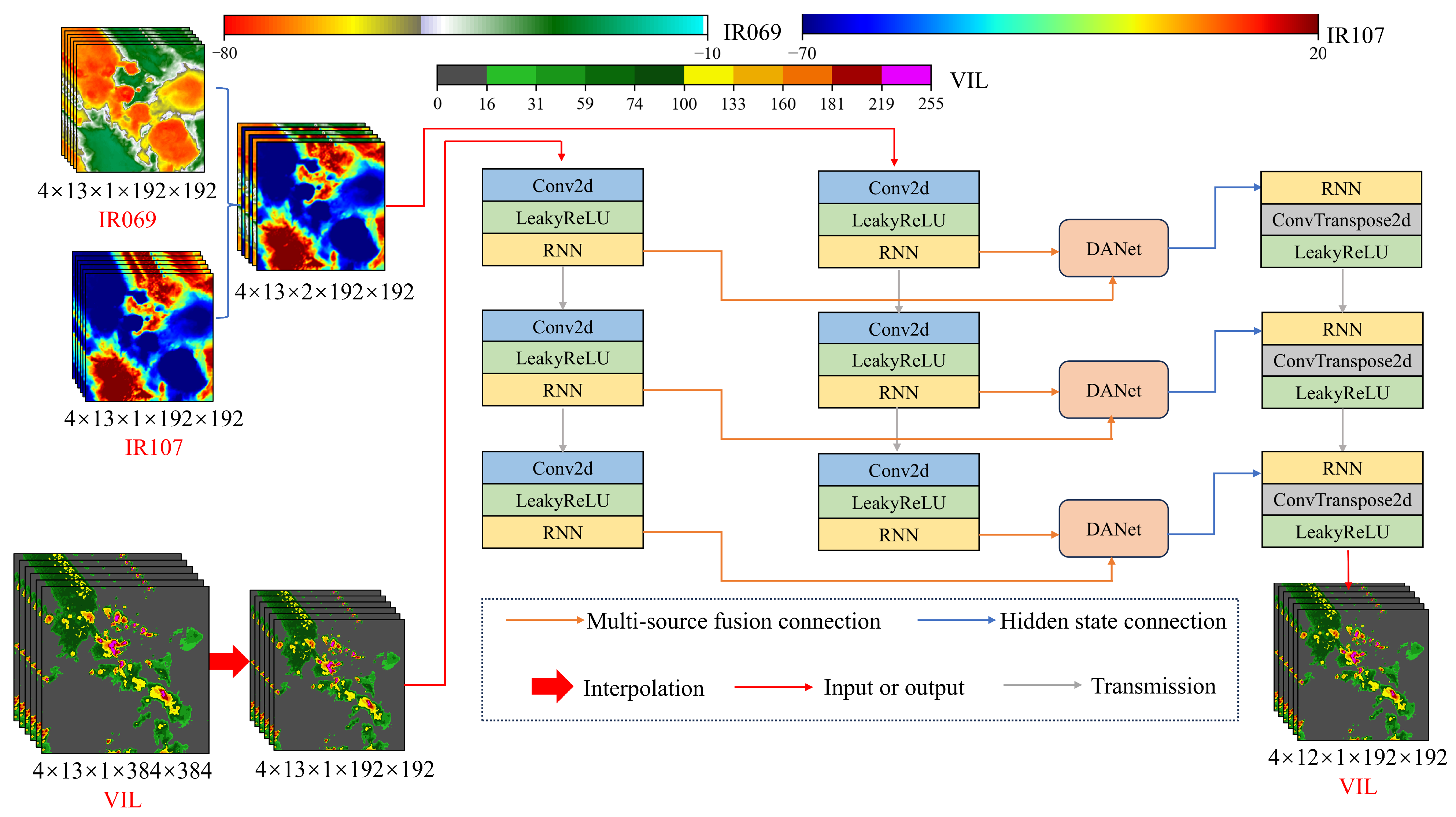
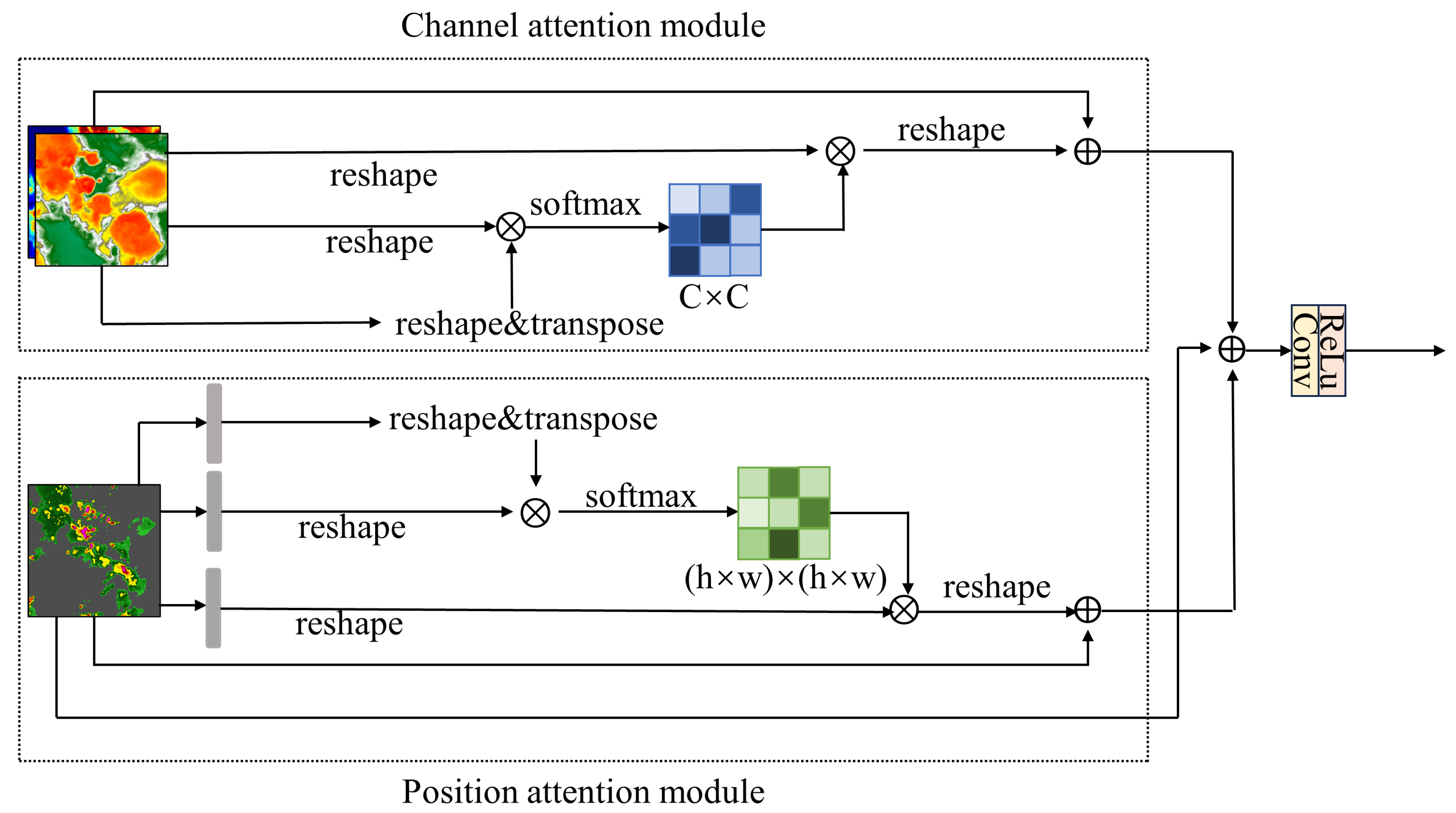
2.1. Model Introduction

We developed DA-RNN, as shown in Figure 1, which fuses satellite infrared and weather radar VIL data. This model combines an encoder–predictor model based on an RNN with a DANet feature extraction network. Traditional DANets generally use ResNet [40] as the backbone for feature extraction. However, nowcasting is a spatiotemporal forecasting problem. ResNet is mainly based on the CNN structure and has a weak ability to extract temporal information. Therefore, we used an RNN-based encoder–predictor network as the backbone structure. The difference between the model and the traditional encoder and predictor is that the encoder adopts a dual input method. The weather radar VIL and satellite IR images are placed in two different input ends, then the feature extraction DANet is introduced at the connection between the encoder and the predictor to fuse the two sources of information through the feature extraction network. This combination fully considers the characteristics of the RNN-based encoder–predictor network in extracting temporal features, applying the strengths of the fusion with the DANet multiple-attention mechanism to increase the warning rate. Finally, the fused information is passed to the predictor module to obtain the final predicted weather radar VIL map.

The proposed DA-RNN model is a multiple-output encoder–predictor model. Its main components are convolution, deconvolution, and leakyReLU activation functions, an RNN network, and a DANet feature extraction network. The convolution and deconvolution functions respectively act as downsampling and upsampling layers that extract the spatial features from the image. The leakyReLU activation function uses a certain slope in the negative part to avoid the gradient vanishing problem that affects neurons during training, and also helps to strengthen the nonlinear fitting relationship of the model [41]. We chose the TrajGRU [21] and ConvLSTM [20] networks in the RNN because they represent the two basic RNN networks, namely, the GRU and LSTM modules. The GRU module differs in structure from the LSTM module in that the GRU module has one less forget gate than the LSTM module. Therefore, the performance of the two different models needs to be verified. Figure 1 shows the technical route in the experiment, which involved randomly selecting 25 consecutive radar VIL images and the first 1h (13 images) of IR107 and IR069 as the training set, then inputting them into the DA-RNN for training to obtain the predicted 12 images. Finally, the loss function was updated to sequentially train the models until the complete dataset was trained.

The module used for fusing the weather radar VI and satellite infrared data features consists of a network that combines spatial feature extraction and DANet channel feature extraction, as shown in Figure 2. Satellite infrared information is extracted from two different channels through the channel attention module, while radar spatial information is extracted through the spatial attention module. Then, the extracted features are accumulated to obtain the fused features. The information integration capability of DANet’s dual attention mechanism is used to fuse satellite infrared and radar information, helping the network to understand complex scenes and increase its segmentation accuracy. The dual attention mechanism reduces the model’s sensitivity to noise and interference by focusing on important spatial and channel features, improving the model’s generalization ability. However, we ultimately chose to predict weather radar images. We added a residual network to increase the warning rate obtained when using weather radar images in order to increase the weight of the weather radar data. Finally, we added a 1 × 1 convolution at the end of the model to help the model fuse cross-channel features and extract high-dimensional features. The model uses a nonlinear activation function to improve its nonlinear representation ability.

To analyze the DANet model, we input the satellite’s infrared feature vector of shape size $C\times H\times W$ (where C represents the number of channels, H represents the height, and W represents the width) into the channel feature extraction network, then reshaped it to size $C\times N$ (where $N=H\times W$). Then, we perform matrix multiplication with its transpose and apply the softmax layer to obtain the channel feature attention map X$\in {\mathbb{R}}^{C\times C}$. The formula is as follows:

$$x_{ji}={\displaystyle \frac{exp(A_i·A_j)}{{\sum }_{i=1}^{C}exp(A_i·A_j)}}$$

(1)

where $x_{ji}$ represents the influence of the i-th channel on the j-th channel and A represents the initial input feature. Following matrix multiplication of X and A, we reshape the result into ${\mathbb{R}}^{C\times H\times W}$ and multiply the result by a scale parameter $\beta$ (learning weights from 0). A sum operation with A is then performed one-by-one to obtain the final output ${\mathbb{R}}^{C\times H\times W}$. The formula is as follows:

$$E_j=\beta \sum _{i=1}^C\left(x_{ji}{A}_i\right)+A_j.$$

(2)

We input the weather radar precipitation feature vector A with a shape size of $C\times H\times W$ into the spatial feature extraction network, then use convolution to generate two new feature maps B and C, which are reshaped to a size of $C\times N$. Following matrix multiplication on the transpose of C and B, the softmax layer is applied to perform spatial attention mapping to $S\in {\mathbb{R}}^{N\times N}$. The specific formula is as follows:

$$s_{ji}={\displaystyle \frac{exp(B_i·C_j)}{{\sum }_{i=1}^{N}exp(B_i·C_j)}}$$

(3)

where $s_{ji}$ represents the influence of the i-th position on the j-th position. The more similar the features of the two positions, the stronger their correlation. We input feature A into the convolution layer to generate a new feature map $D\in {\mathbb{R}}^{C\times H\times W}$, which we reshape; then, we perform matrix multiplication on the device of D and S to obtain ${\mathbb{R}}^{C\times H\times W}$, which we multiply by the scale parameter $\alpha$. After this, we use an element-wise sum operation with feature A to finally obtain $E\in {\mathbb{R}}^{C\times H\times W}$. The formula is as follows:

$$E_j=\alpha \sum _{i=1}^N\left(s_{ji}{D}_i\right)+A_j.$$

(4)

2.2. Experimental Data

The SEVIR dataset [42] used in this experiment includes observational data from the United States GOES-16 satellite, while the weather radar data are provided by the WSR-88D (NEXRAD) radar national network. This dataset is temporally and spatially aligned, and contains more than 10,000 weather events. Each weather event contains a 4-h 384 km × 384 km image sequence with a temporal resolution of 5 min. This rich dataset includes five different data types, as detailed in

Table 1. SEVIR dataset details.

Data Type	Description	Sensor	Spatial Resolution	Patch Size
VIS	Visible satellite imagery	GOES-16 C02 0.64 μm	0.5 km	768 × 768
IR069	Infrared Satellite imagery (mid-level water vapor)	GOES-16 C09 6.9 μm	2 km	192 × 192
IR107	Infrared Satellite imagery (clean longwave window)	GOES-16 C13 10.7 μm	2 km	192 × 192
VIL	NEXRAD radar mosaic of VIL	Vertically Integrated Liquid (VIL)	1 km	384 × 384
Lightning	Intercloud and cloud to ground lightning events	GOES-16 GLM flashes	8 km	N/A

, including four types of satellite data. However, in the experiment we only used two types of satellite infrared data, as our primary focus was on the physical relationship between temperature and precipitation. The VIS and Lightning data products do not have any direct correlation with precipitation and temperature. Moreover, the Lightning product has a larger spatial resolution, which can lead to significant errors after standardization. Therefore, we selected only the IR107 and IR069 data, which contain satellite temperature information. Additionally, we used VIL data from the NEXRAD radar sensor to predict precipitation.

We used the IR069 and IR107 data to analyze the VIL data; the VIL images were stored as integers in the range of 0–254, with 255 representing the missing part. We converted the pixel value into VIL (unit) using the following formula, which shows that the pixel value was positively correlated with the VIL value.

$$f\left(X\right)=\left\{\begin{array}{cc}0\hfill & if(X\le 5)\hfill \\ {\displaystyle \frac{X-2}{90.66}}\hfill & if(5<X\le 18)\hfill \\ {\displaystyle \frac{\exp (X-83.9)}{38.9}}\hfill & if(18<X\le 254)\hfill \end{array}\right.$$

(5)

The unit of the IR069 and IR107 data is °C, and the data are linearized for efficient storage. Both are multiplied by 100; therefore, we performed data reduction during the experiment. In addition, because the units of the data from the different sources were different, we used 0–1 normalization on to unify the range in order to improve the fusion of the satellite infrared and radar VIL data types and prevent the model from overfitting.

Because the spatial resolution of the VIL, IR107, and IR069 data in the SEVIR dataset are different, we reduced the complexity of the model by applying linear interpolation of the VIL data to a spatial resolution of 2 km and a picture size of 192 × 192 pixels. Finally, we performed data enhancement operations on the dataset to enhance its multiple-source nature. Given the time-dependent nature of the time series, we chose the sliding window method for the data enhancement operation, using a sliding window operation with a window size of 25 and a step size of 12 for the 49 frames of each event and dividing the four hours into three instances. This helped with the model training and testing processes and increased the robustness of the model, preventing possible overfitting due to the small amount of input data.

The SEVIR dataset mainly contains two types of data: randomly selected data and data based on storm events. Therefore, we selected random data and storm data from 1 January 2018 to 30 June 2019 and randomly divided them into training and validation sets according to the ratio of 8:2. Storm data from 1 July 2019 to 30 December 2019 was used as the test set. However, some events in the dataset are missing. In order to prevent noise from being introduced into the model training process, we deleted the missing events during the model training. In addition, the SEVIR dataset is integrated based on the radar system of the entire United States. Spatially, it is more comprehensive than the images produced by a single radar sensor.

All models in the experiment were implemented on the Pytorch framework and run on an NVIDIA GeForce RTX 4090 graphics card with 24 GB of video memory (NVIDIA, Santa Clara, CA, USA). The MSE loss function was used in all models [43], with Adam as the optimizer. The minimum and maximum values of the optimizer momentum were 0.9 and 0.99, respectively. The learning rate was 0.0001, and the learning strategy was set to cosine annealing. We set 50 as the maximum number of training sessions and 5 as the early stopping number. The specific experimental settings are shown in

Table 2. Experimental configuration and setup.

Name	Configuration
Learning Framework	Pytorch 1.8
Graphics card	NVIDIA GeForce RTX 4090
Graphics memory	24 GB
Learning rate	0.0001
Learning strategy	Cosine AnnealingLR
Optimizer	Adam
Loss function	MSE

.

2.3. Evaluation Methods

We used the indicators in

Table 3. Evaluation indicators.

Index	Equation	Optimal Value
Mean Absolute Error (MAE)	${\displaystyle \frac{1}{N}}{\sum }_{n=1}^N{\sum }_{i=1}^{192}{\sum }_{j=1}^{192}\left|x_{n,i,j}-{\widehat{x}}_{n,i,j}\right|$	0
Mean Squared Error (MSE)	${\displaystyle \frac{1}{N}}{\sum }_{n=1}^N{\sum }_{i=1}^{192}{\sum }_{j=1}^{192}{\left(x_{n,i,j}-{\widehat{x}}_{n,i,j}\right)}^2$	0
Peak Signal-to-Noise Ratio (PSNR)	$10{\log }_{10}\left({\displaystyle \frac{MA{X}^2}{MSE}}\right)$	$+\infty$
Structural Similarity Index Measure (SSIM)	${\displaystyle \frac{\left(2{\mu }_x{\mu }_y+c_1\right)\left(2{\sigma }_{xy}+c_2\right)}{\left({\mu }_x^2+{\mu }_y^2+c_1\right)\left({\sigma }_x^2+{\sigma }_y^2+c_2\right)}}$	1
Continuous Ranked Probability Score (CRPS)	$\int {[CDF\left(x\right)-H(x-y)]}^{2}dx$	0
Sharpness	${\displaystyle \frac{1}{191\times 191}}{\sum }_{i=1}^{191}{\sum }_{j=1}^{191}{(y_{i+1,j}-y_{i,j})}^2+{(y_{i,j+1}-y_{i,j})}^2$	$+\infty$
Critical Success Index (CSI)	${\displaystyle \frac{TP}{TP+FN+FP}}$	1
False Alarm Rate (FAR)	${\displaystyle \frac{FP}{TP+FP}}$	0
Heidke Skill Score (HSS)	${\displaystyle \frac{TP\times TN-FN\times FP}{(TP+FN)(FN+TN)+(TP+FN)(FP+TN)}}$	1
Fraction Skill Score (FSS)	$FSS=1-FBS/{FBS}_{worst}$$FBS={\displaystyle \frac{1}{N}}{\sum }_{i=1}^N{(f\left(m_i^s\right)-f\left(o_i^s\right))}^2$	1

Note: N is the total number of outputs, $x_{n,i,j}$ represents the size of the true value of the n-th image at weather radar image position $\left(i,j\right)$, and ${\widehat{x}}_{n,i,j}$ represents the size of the predicted value at the same position; $MAX$ represents the maximum value of all pixel values; ${\mu }_x$ and ${\mu }_y$ represent the average brightness of the real image and the predicted image, respectively; ${\sigma }_x^2$ and ${\sigma }_y^2$ represent the standard deviation of the brightness of the real value image and the predicted image, respectively; ${\sigma }_{xy}$ represents the brightness covariance of the two images; $c_1$ and $c_2$ are stability parameters; $CDF\left(X\right)$ denotes the probability distribution of the real images; $y_{i,j}$ represents the size of the predicted value of weather radar echo image position $\left(i,j\right)$; true positive ($TP$) represents prediction = 1, true value = 1; false negative ($FN$) represents prediction = 0, true value = 1; false positive ($FP$) represents prediction = 1, true value = 0; true negative ($TN$) represents prediction = 0, true value = 0; $f\left(m_i^s\right)$ and $f\left(o_i^s\right)$ in FBS represent the proportions of the number of grid points for which the model’s forecasts and the observations respectively exceed the precipitation threshold of t in the neighborhood scale s surrounding grid point i; N is the number of grid points in the study area; and ${FBS}_{worst}$ is the sum of the squares of all the duty scores computed for the forecasts and observations.

to evaluate the prediction ability of each model. Specifically, we used the MAE (mean absolute error) and MSE (mean squared error) as evaluation indicators in the regression problems to evaluate the differences in the pixel values between the model-predicted images and the real observed images. We used the SSIM (structural similarity index measure) and PSNR (peak signal-to-noise ratio) to analyze the structural similarity between the predicted images and the real images. We also used the changes in the quality of the predicted images to analyze the quality of the predicted images in more detail. We used the CRPS (continuous ranked probability score) and sharpness to assess the probability distribution and the clarity of the predicted image. Because the attention paid to different precipitation conditions differs in meteorological work, evaluating the prediction performance of the model under different thresholds is valuable for echo extrapolation warnings. For this purpose, we chose several evaluation indicators that are commonly used in binary classification problems: CSI (critical success index), FAR (false alarm rate), and HSS (Heidke skill score). We used these indicators to evaluate the following pixel values: 31, 74, 133, and 181 [44]. Finally, we added the FSS (fraction skill score) to evaluate the different pixel values, as the spatial retention of the predicted images is also important.

3. Results and Discussion

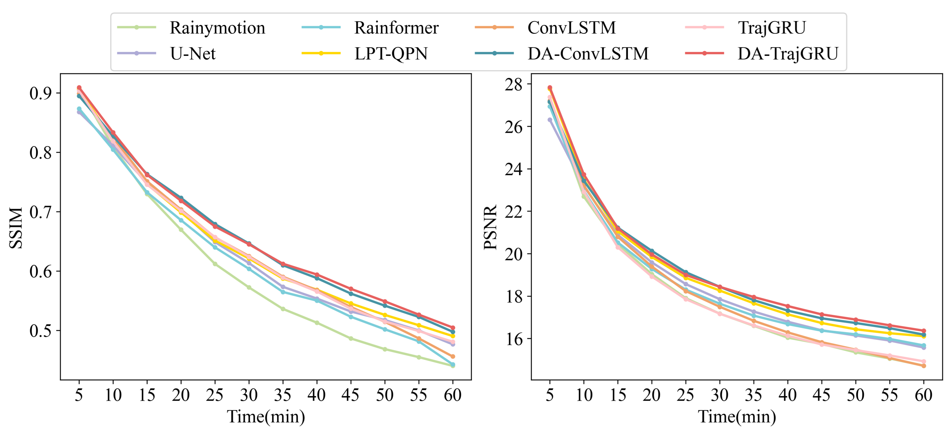
3.1. Test Set Results

To verify the proposed method fusing satellite infrared data and weather radar VIL data for use in short-term precipitation forecast and test the performance of our DA-RNN model, we selected five models for comparison. For comparison with the proposed DA-RNN, we selected a traditional RNN model as well as the RNN-based ConvLSTM and TrajGRU models In addition, we selected the CNN-based U-Net model. This choice can help to assess the difference in performance between CNN and RNN models. As the most basic convolution structure, U-Net is often used for comparison and to verify the performance of models on the SEVIR dataset. Third, we selected Rainformer [45] and LPT-QPN [46] (lightweight physics-informed transformer for quantitative precipitation nowcasting), both of which are based on the transformer attention mechanism, in order to validate the performance differences between models utilizing the transformer attention mechanism and the DANet attention mechanism. Both of these models have demonstrated their performance on the respective datasets. Finally, we selected the DenseRotation model [47] (Rainymotion) from the rainymotion library to verify the difference between methods based on deep learning and those based on traditional learning. This model tracks precipitation fields based on optical flow technology and extrapolates precipitation fields based on a constant vector advection scheme. This model has performance comparable to or better than that of the RADVOR (radar real-time forecast) model and is applicable to a wide range of precipitation events.

The specific differences due to the differences in the specific parameters of the model in the experimental environment and the original text are shown in

Table 4. Implementation details for the baseline models.

Model	Details	Official Configuration	Our Adaptations
U-Net	Input length	7	13
	Output length	12	12
Rainformer	Input length	9	13
	Output length	9	12
ConvLSTM	Loss function	Balanced MSE	MSE
	Input length	5	13
	Output length	20	12
TrajGRU	Loss function	Balanced MSE	MSE
	Input length	5	13
	Output length	20	12

.

We chose the model with the smallest loss function after each iteration and tested this model on the test set to validate the performance of the DA-RNN model. The average MSE, MAE, SSIM, and PSNR results of each model on the test set with 192 × 192 pixel images are shown in

Table 5. MSE↓, MAE↓, SSIM↑, and PSNR↑ of the eight precipitation models on the test set. The best results are indicated in bold.

Algorithm	MSE↓	MAE↓	SSIM↑	PSNR↑
Rainymotion	356	1403	0.7161	22.179
U-Net	332	1437	0.7335	22.384
Rainformer	321	1417	0.7316	22.578
LPT-QPN	318	1384	0.7406	22.71
ConvLSTM	321	1383	0.7467	22.643
DA-ConvLSTM	297	1308	0.7552	22.906
TrajGRU	321	1390	0.7476	22.645
DA-TrajGRU	291	1301	0.7572	23.033

. The table shows that the CNN-based U-Net and the Rainymotion model based on the optical flow method had relatively large MSE and MAE values and relatively small SSIM and PSNR values, which is due to the weak ability of the CNN to extract temporal and strong precipitation information. The poor performance of the Rainymotion model can be attributed to the optical flow method extracting the highly complicated and nonlinear strong convective weather features. The MSE and MAE values of the Rainformer and LPT-QPN models were larger than those of the DA-RNN model, and their SSIM and PSNR values were smaller, which verifies the performance of our DA-RNN model. Finally, the SSIM and PSNR of the DA-RNN model were the largest, showing that the images predicted by the DA-RNN model were the closest to the observed values in terms of structure, brightness, and values. Additionally, the MSE and MAE values of the DA-ConvLSTM and DA-TrajGRU models incorporating satellite infrared data were low compared with those of the traditional ConvLSTM and TrajGRU models based on the extrapolation of weather radar echoes; the MSE was reduced by $7.4\%$ and $9.3\%$, respectively, while the MAE was reduced by $5.4\%$ and $6.4\%$, respectively, demonstrating that the DA-RNN model can produce higher-accuracy precipitation predictions by including satellite infrared data.

In meteorological research, the growth patterns of various metrics with increasing lead time are also very important; therefore, we present images showing the changes in MSE and MAE for each model on the test set over time. From Figure 3, it can be observed that the performance of the DA-RNN model incorporating infrared satellite data and the DANet network model improves significantly as time increases, particularly the DA-TrajGRU model. As the lead time increases, the performance gap between the DA-TrajGRU model and the other models widens, indicating better performance.

We used the CRPS (continuous ranked probability score) to evaluate the difference between the predicted and actual probability distributions in order to further verify the performance of the models. We also considered the sharpness metric to evaluate the clarity and details of the predicted images. The Rainymotion model was not evaluated because the optical flow method is based on the movement of pixel points for radar echo extrapolation. The performance of each model on the test set is shown in

Table 6. CRPS↓ and Sharpness↑ of the eight precipitation models on the test set. The best results are indicated in bold.

Algorithm	CRPS↓	Sharpness↑
U-Net	5.895	46.83
Rainformer	5.789	47.41
LPT-QPN	5.701	43.78
ConvLSTM	5.789	49.46
DA-ConvLSTM	5.555	50.68
TrajGRU	5.881	47.95
DA-TrajGRU	5.632	51.20

. DA-ConvLSTM had the smallest CRPS, followed by DA-TrajGRU, which led us to the conclusion that the probability distributions of the forecasts of the DA-RNN model were the most similar to those of the actual images. The sharpness was highest for DA-TrajGRU, which predicted a clearer picture with more details. Both metrics led us to the conclusion that the DA-RNN model performed best when including satellite infrared data.

Finally, because meteorologists often focus on model performance under different precipitation thresholds, we provide the CSI, FAR, HSS, and FSS values of the different models on the test set at different pixel value thresholds (VIL values positively correlated with pixel values) of 31, 74, 133, and 181 (

Table 7. Performance in terms of CSI↑ values on the test set under different precipitation thresholds. The best results are indicated in bold.

Algorithm	Pixel ≥ 31	Pixel ≥ 74	Pixel ≥ 133	Pixel ≥ 181
Rainymotion	0.6305	0.5176	0.2986	0.1793
U-Net	0.6509	0.5562	0.3717	0.2443
Rainformer	0.6555	0.5607	0.3677	0.2403
LPT-QPN	0.6594	0.5661	0.3753	0.2423
ConvLSTM	0.6626	0.5632	0.3796	0.2488
DA-ConvLSTM	0.6732	0.5728	0.3821	0.2496
TrajGRU	0.6608	0.5665	0.3841	0.2537
DA-TrajGRU	0.6751	0.5783	0.3897	0.2523

,

Table 8. Performance in terms of FAR↓ values on the test set under different precipitation thresholds. The best results are indicated in bold.

Algorithm	Pixel ≥ 31	Pixel ≥ 74	Pixel ≥ 133	Pixel ≥ 181
Rainymotion	0.2343	0.3273	0.5469	0.6778
U-Net	0.2901	0.3743	0.5026	0.5274
Rainformer	0.2821	0.3599	0.4928	0.5342
LPT-QPN	0.2724	0.3559	0.4869	0.5195
ConvLSTM	0.2761	0.3688	0.4944	0.5337
DA-ConvLSTM	0.2561	0.3551	0.4801	0.5175
TrajGRU	0.2849	0.3636	0.4906	0.5073
DA-TrajGRU	0.2630	0.3468	0.4727	0.4896

,

Table 9. Performance in terms of HSS↑ values on the test set under different precipitation thresholds. The best results are indicated in bold.

Algorithm	Pixel ≥ 31	Pixel ≥ 74	Pixel ≥ 133	Pixel ≥ 181
Rainymotion	0.7042	0.6173	0.4055	0.2620
U-Net	0.7198	0.6537	0.4635	0.3483
Rainformer	0.7242	0.6583	0.4885	0.3425
LPT-QPN	0.7291	0.6635	0.4962	0.3435
ConvLSTM	0.7307	0.6596	0.5017	0.3534
DA-ConvLSTM	0.7432	0.6705	0.5051	0.3538
TrajGRU	0.7291	0.6634	0.5071	0.3583
DA-TrajGRU	0.7441	0.6762	0.5137	0.3561

and

Table 10. Performance in terms FSS↑ values on the test set under different precipitation thresholds. The best results are indicated in bold.

Algorithm	Pixel ≥ 31	Pixel ≥ 74	Pixel ≥ 133	Pixel ≥ 181
Rainymotion	0.7516	0.6535	0.4253	0.2690
U-Net	0.7718	0.6928	0.5127	0.3543
Rainformer	0.7752	0.6959	0.5068	0.3484
LPT-QPN	0.7781	0.7004	0.5144	0.3493
ConvLSTM	0.7805	0.6985	0.5202	0.3593
DA-ConvLSTM	0.7891	0.7074	0.5228	0.3596
TrajGRU	0.7792	0.7008	0.5253	0.3641
DA-TrajGRU	0.7907	0.7119	0.5311	0.3613

). The CSI, HSS, and FSS constantly decreased with the increase in precipitation intensity, while the FAR constantly increased. This is a problem that meteorologists must overcome, and is caused by lack of information about the heavy precipitation area in the image. For this reason, less information is extracted during the deep learning process, resulting in poor prediction ability [48,49].

The CSI and HSS of DA-TrajGRU were the largest, indicating more accurate predictions. The FSS of DA-TrajGRU was relatively large for the individual thresholds, indicating that the spatial structure of its predicted images was highly preserved. Additionally, the FAR value of the DA-TrajGRU model was relatively low, indicating that the rate of false positives was low. This result demonstrates that the DA-TrajGRU model had the best performance. Finally, the growth in each index was analyzed for the DA-TrajGRU model. The results showed that while the CSI, HSS, and FSS did not considerably improve, the FAR substantially decreased. This can be attributed to the introduction of satellite infrared data, which increases the amount of information learned by the model, thereby helping to prevent the model from overestimating some pixel values. In the results, some fuzzy areas were directly predicted into the area of larger pixel values.

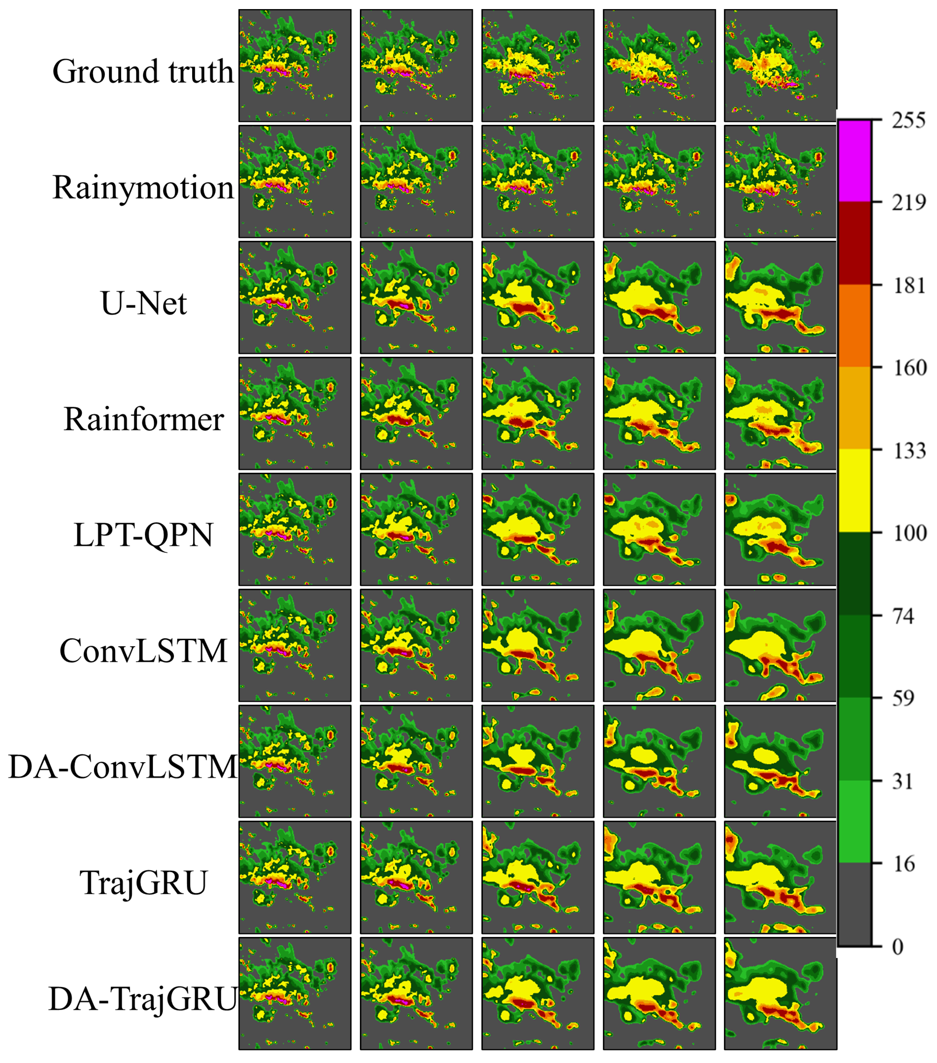
3.2. Case 1: Visualization of a Flash Flood

To further examine the early warning ability of the model, we randomly selected two storm events for visual analysis. First, we selected a flash flood that occurred during 20:15–22:15 (UTC) on 7 July 2019. The longitude and latitude in the lower left corner of the picture are 35.22866374° and −86.26886469°, respectively, while the longitude and latitude in the upper right corner are 38.10467693° and −81.34818572°, respectively. Figure 4 visualizes the images predicted by each model. The figure shows that as the prediction time increases, the details in the predicted image decrease and the differences between the predicted and real images increase. This is an unavoidable problem in meteorology. In addition, we analyzed the overall performance of each model. Rainymotion had higher resolution; however, the specific location of the storm cell and the shape of the envelope were different from those in the observed image. The U-Net model underestimated the area with strong pixel values, while Rainformer and LPT-QPN overestimated the pixel values to a certain extent, with many large pixels appearing that were not present in the actual observed weather radar VIL images. Finally, ConvLSTM overestimated the pixel values of the VIL images to a certain extent, predicting large pixel values in parts of the observed image that had extremely low pixel values. On the other hand, the DA-ConvLSTM model, which incorporates satellite infrared data, accurately predicted the ares with lower pixel values, and the location of its large pixel values was closest to the observed value. Similarly, the TrajGRU model without satellite infrared data overestimated the predicted pixel values, whereas the DA-TrajGRU model incorporating satellite infrared data was able to learn the features of low-value pixels, and the range of its high pixel values was the closest to the observed value.

Figure 5 provides the MSE and MAE of each model in Case 1 over time to verify the relationship between the predicted and observed images. The figure shows that the DA-ConvLSTM and DA-TrajGRU models had lower MAE and MSE than the other models over time, and their predicted images were closest to the observed image. These results prove the superior performance of DA-RNN, especially the DA-TrajGRU model, which performed the best. This corresponds to the results regarding the performance of each model under different thresholds in Case 1.

Figure 6 provides the CSI, FAR, and HSS results of the different models under different pixel thresholds over time. The figure shows that all indicators deteriorate as the threshold increases, which is consistent with the visual results. In addition, we analyzed the results under different thresholds. When the threshold was small, the CSI and HSS of the DA-ConvLSTM model were the largest and its FAR was the smallest. When the threshold was greater than or equal to 74, the performance of the DA-TrajGRU model was more accurate. This result proves the superior performance of the DA-RNN model. We noticed that the performance of the DA-RNN model improved more than that of the other models over time, which is because the introduction of satellite infrared information provides the model with more learnable features. Finally, the FAR of the DA-RNN model was notable. The introduction of satellite infrared information provides the model with more information about the areas in the image that experience faster changes, thereby avoiding overestimation of some pixel values, which is consistent with the results on the test set.

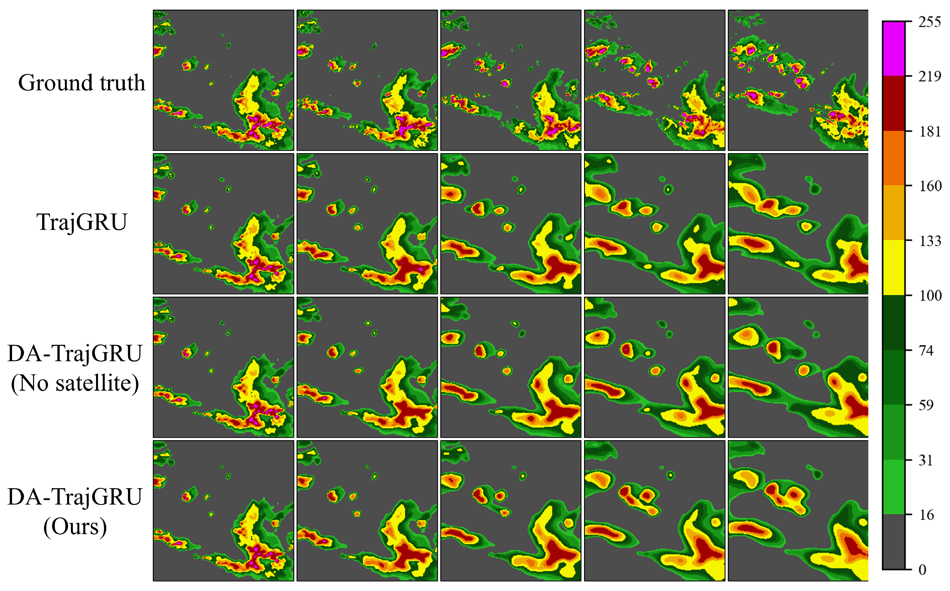
3.3. Case 2: Visualization of a Thunderstorm with High Winds

For Case 2, we randomly selected a thunderstorm wind event that occurred at 20:20–22:20 (UTC) on 21 July 2019 to further verify the results. The latitude and longitude in the lower left corner of the image are 36.96008315° and −81.46989148°, while those in upper right corner are 39.59926506° and −76.21631393°, respectively. The specific visualizations of the predictions of each model are shown in Figure 7. It can be seen that the VIL images predicted by the TrajGRU and ConvLSTM models overestimated some weak pixel value areas, while the DA-RNN model considering satellite infrared data did not have this problem. The strong pixel area in the figure shows that the shape and pixel values of DA-RNN were closer to the true value. Based on these results, we can conclude that the DA-RNN model performed the best.

Figure 8 provides specific data to verify the results obtained from the visualization. The figure shows the CSI, FAR, and HSS results of the different models over time under different pixel value thresholds. These results indicate that the DA-RNN model performed relatively well under different thresholds; its CSI and HSS were the largest, and its FAR was the smallest. In addition, the FAR of the DA-RNN model was always the best among the deep learning models. Therefore, we can conclude that the introduction of satellite infrared data helps the DA-RNN model to obtain more spatiotemporal information, thereby preventing low pixel values from being mistakenly reported as high pixel values. This conclusion is consistent with the results from Case 1.

Figure 9 provides images of the SSIM and PSNR in Case 2 for the different models over time, helping to more intuitively display the difference between the ground-observed VIL images and the predicted images. The values of the DA-TrajGRU model are relatively large, followed by the DA-ConvLSTM model. This proves that the image predicted by the DA-RNN model in Case 2 was the most similar to the observed VIL image in terms of structure, brightness, and value.

3.4. Discussion

We conducted an ablation experiment to verify the impact of satellite infrared data and DANet on prediction accuracy. Using the test set, we tested the TrajGRU network with only weather radar VIL data as the input along with the DA-TrajGRU network with weather radar VIL data as input on both ends (DA-TrajGRU (No satellite)) and the DA-TrajGRU model with weather radar VIL data and satellite infrared data as input (DA-TrajGRU (Ours)). The SSIM, PSNR, MAE, and MSE are listed in

Table 11. SSIM↑, PSNR↑, MAE↓, and MSE↓ performance of the three models on the test set. The best results are indicated in bold.

Algorithm	SSIM↑	PSNR↑	MSE↓	MAE↓
TrajGRU	0.7476	22.645	321	1390
DA-TrajGRU (No satellite)	0.7521	22.845	308	1340
DA-TrajGRU (Ours)	0.7572	23.033	291	1301

. The table shows that the DA-TrajGRU model with infrared data had the largest SSIM and PSNR along with the smallest MSE and MAE. Therefore, the DA-TrajGRU model with satellite infrared data, produced the largest increase in warning rate for precipitation nowcasting. In addition, the integration of DANet strengthened the warning ability of the model to a certain extent compared with the traditional encoder predictor network. Finally, the overall analysis shows that the integration of satellite infrared data with the DANet model increases the warning rate of precipitation nowcasting.

The performance of CSI-M (mean CSI), FAR-M (mean FAR), HSS-M (mean HSS), and FAR at different thresholds is shown in

Table 12. Quantitative mean values and FAR↓ for various levels on the test set. The best results are indicated in bold.

Algorithm	CSI-M↑	FAR-M↓	HSS-M↑	FAR-31↓	FAR-74↓	FAR-133↓	FAR-181↓
TrajGRU	0.4662	0.4116	0.5644	0.2849	0.3636	0.4906	0.5073
DA-TrajGRU (No satellite)	0.4701	0.4007	0.5692	0.2723	0.3536	0.4861	0.4908
DA-TrajGRU (Ours)	0.4738	0.3931	0.5725	0.2631	0.3468	0.4727	0.4896

, demonstrating the effect of incorporating satellite infrared data with DANet on precipitation prediction accuracy. After adding DANet and satellite infrared data, both CSI-M and HSS-M increased, while FAR-M decreased, with FAR showing a consistent reduction across different thresholds. Thus, we can verify that the use of DANet and satellite infrared data enhances the warning rate in near-term precipitation forecasting.

To visually analyze the impact of satellite infrared data and the DANet network on the warning rate, we randomly selected a hail event from the test set. The selected event occurred from 21:47 to 23:47 (UTC) on 5 August 2019. The latitude and longitude in the lower left corner of the image are 42.73538143° and −94.47546042°, respectively, while those in the upper right corner are 45.94886431° and −89.30948182°. The visualization results of each model are shown in Figure 10. From the figure, it can be seen that the predictions are closer to the true image after adding the DANet network, with more accurate shapes and contours compared to the results from the TrajGRU network. Furthermore, the predictions after incorporating infrared satellite data show intensity and range that are closer to the ground truth values than those obtained with just the DANet network. This validates the conclusion that both infrared satellite data and the DANet network enhance the warning rate in the test set results.

Finally, we considered the computational cost of the models. The model training and inference times and the computational cost of training for the three cases in the ablation experiments are shown in

Table 13. Computational and reasoning costs of the three models.

Algorithm	Training Time per Epoch (min)	GPU Memory (MB)	Inference Time per Case (S)
TrajGRU	50	10417	0.223
DA-TrajGRU (No satellite)	55	15672	0.228
DA-TrajGRU (Ours)	100	19707	0.324

. The addition of DANet did not affect the computational or inference efficiency of the model, while the addition of the satellite infrared data increased both computational cost and time. This is a problem facing multiple-source information fusion. In the future, we will consider incorporating reinforcement learning to reduce the computation and reasoning time.

The results of the ablation experiment verify that both satellite infrared data and DANet increase the warning rate in precipitation nowcasting. However, as with other deep learning models, the details of the predicted image are increasingly lost as the prediction time increases. In addition, due to the widespread use of the MSE loss function in deep learning, the predicted image may be too smooth, resulting in low resolution. Therefore, in future work we will consider introducing a GAN (generative adversarial network), which has higher resolution, in order to increase the resolution of the predicted image.

4. Conclusions

In this paper, we have developed the DA-RNN model, which combines an RNN encoder–predictor with DANet. The resulting model effectively integrates satellite infrared data and weather radar VIL data by leveraging the multi-attention mechanism of DANet, thereby enriching the network with enhanced spatiotemporal information. Additionally, the incorporation of temperature information through neural networks and the microphysical fusion of precipitation data substantially strengthens the early warning accuracy of precipitation forecasts. A comprehensive analysis leads us to the following conclusions:

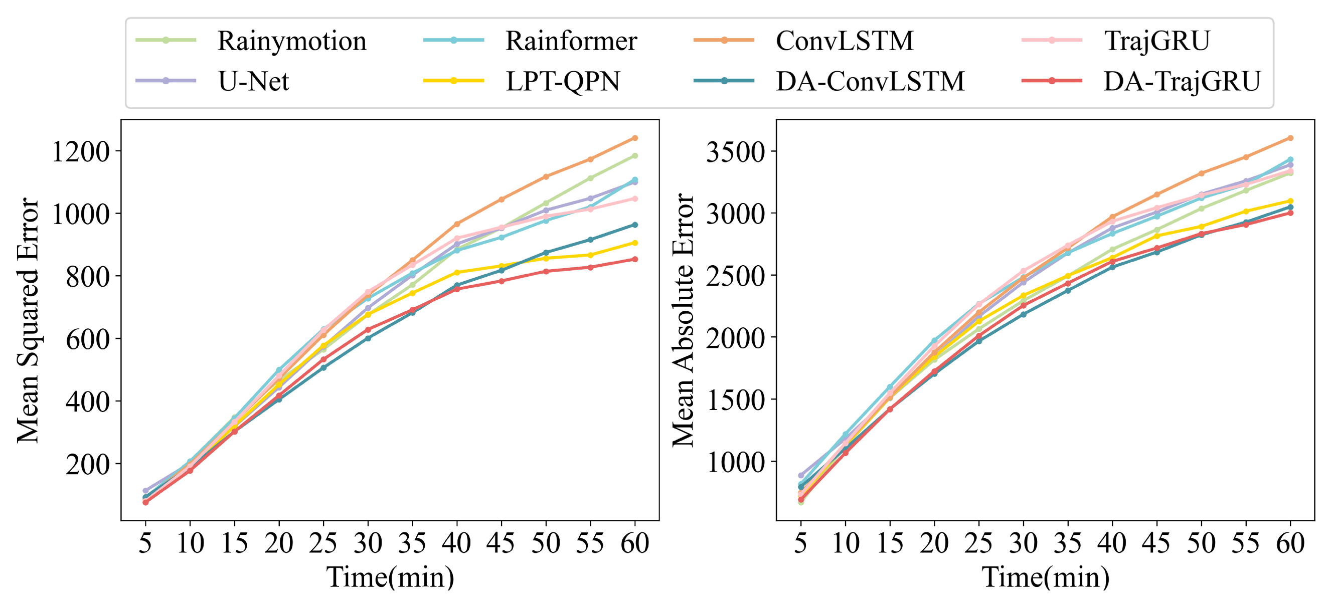
• Enhanced Prediction Performance: The proposed DA-RNN incorporating satellite infrared data demonstrates superior predictive performance compared with traditional RNN models. Specifically, the MSE and MAE of the DA-TrajGRU model were $9.3\%$ and $6.4\%$ lower, respectively, compared with those of the TrajGRU model. Similarly, the DA-ConvLSTM model exhibited $7.4\%$ and $5.4\%$ reductions in the same metrics compared with the ConvLSTM model.
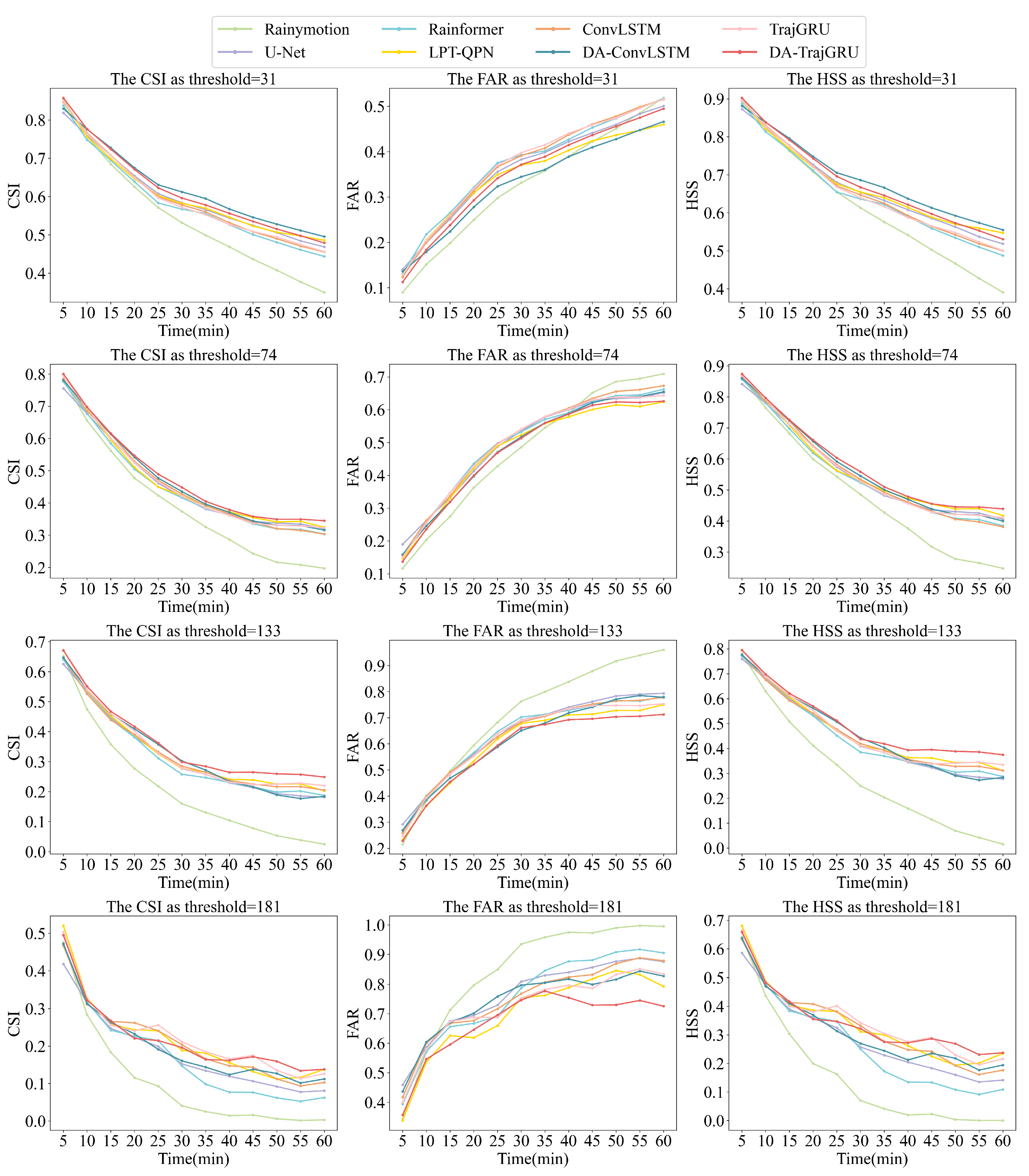
• Robustness Across Thresholds: The proposed model’s performance across various thresholds indicates that the FAR remains robust in deep learning models, whereas the CSI and HSS tend to decline as the threshold increases. This result can be attributed to the limited amount of information extracted from weather radar VIL images with larger pixel thresholds. The integration of satellite infrared data aids in extracting more comprehensive information, helping to mitigate the overestimation of pixel values in certain areas.
• Accuracy in Real-World Scenarios: The DA-RNN model’s predictions closely aligned with real weather radar images in terms of pixel intensity and envelope. Although the Rainymotion optical flow method offers higher resolution, its predicted envelope and storm positions substantially deviated from the actual observations. Similarly, other models may overestimate pixel values due to insufficient temporal information extraction.
• Importance of Satellite Infrared Data: The results of our ablation tests on the proposed DA-RNN model underscore the critical role of combining DANet with RNN in enhancing the warning rate for precipitation nowcasting. Satellite infrared data are indispensable for increasing the accuracy of these forecasts.

While satellite infrared data and DANet demonstrably improved precipitation nowcasting, the spatial and channel extraction capabilities of the attention mechanism network can be enhanced. Thus, future work will explore integrating DANet with a transformer multihead attention mechanism in order to improve the model’s global feature extraction capabilities and further increase the warning rate. Additionally, as weather radar systems and observation methods continue to evolve, incorporating more physical factors could help to further refine the accuracy of the model’s warnings.

References

1. Chowdhury, A.; Egodawatta, P.; McGree, J. Pattern-based assessment of the influence of rainfall characteristics on urban stormwater quality. Water Sci. Technol. 2023, 87, 2292–2303. [Google Scholar] [CrossRef] [PubMed]
2. Xiang, J.; Wang, H.; Li, Z.; Bu, Z.; Yang, R.; Liu, Z. Case Study on the Evolution and Precipitation Characteristics of Southwest Vortex in China: Insights from FY-4A and GPM Observations. Remote Sens. 2023, 15, 4114. [Google Scholar] [CrossRef]
3. Wang, H.; Tan, L.; Zhang, F.; Zheng, J.; Liu, Y.; Zeng, Q.; Yan, Y.; Ren, X.; Xiang, J. Three-Dimensional Structure Analysis and Droplet Spectrum Characteristics of Southwest Vortex Precipitation System Based on GPM-DPR. Remote Sens. 2022, 14, 4063. [Google Scholar] [CrossRef]
4. Zhang, F.; Melhauser, C. Practical and Intrinsic Predictability of Severe and Convective Weather at the Mesoscales. J. Atmos. Sci. 2012, 69, 3350–3371. [Google Scholar]
5. Wang, L.; Dong, Y.; Zhang, C.; Heng, Z. Extreme and severe convective weather disasters: A dual-polarization radar nowcasting method based on physical constraints and a deep neural network model. Atmos. Res. 2023, 289, 106750. [Google Scholar] [CrossRef]
6. Yan, Y.; Wang, H.; Li, G.; Xia, J.; Ge, F.; Zeng, Q.; Ren, X.; Tan, L. Projection of Future Extreme Precipitation in China Based on the CMIP6 from a Machine Learning Perspective. Remote Sens. 2022, 14, 4033. [Google Scholar] [CrossRef]
7. Che, H.; Niu, D.; Zang, Z.; Cao, Y.; Chen, X. ED-DRAP: Encoder–Decoder Deep Residual Attention Prediction Network for Radar Echoes. IEEE Geosci. Remote Sens. Lett. 2022, 19, 1–5. [Google Scholar] [CrossRef]
8. Reinoso-Rondinel, R.; Rempel, M.; Schultze, M.; Tromel, S. Nationwide Radar-Based Precipitation Nowcasting - A Localization Filtering Approach and its Application for Germany. IEEE J. Sel. Top. Appl. Earth Obs. Remote Sens. 2022, 15, 1670–1691. [Google Scholar] [CrossRef]
9. Ehsani, M.; Zarei, A.; Gupta, H.; Barnard, K.; Lyons, E.; Behrangi, A. NowCasting-Nets: Representation Learning to Mitigate Latency Gap of Satellite Precipitation Products Using Convolutional and Recurrent Neural Networks. IEEE Trans. Geosci. Remote Sens. 2022, 60, 1–21. [Google Scholar] [CrossRef]
10. Ozkaya, A. Assessing the numerical weather prediction (NWP) model in estimating extreme rainfall events: A case study for severe floods in the southwest Mediterranean region, Turkey. J. Earth Syst. Sci. 2023, 132, 125. [Google Scholar] [CrossRef]
11. Ma, Z.; Zhang, H.; Liu, J. Focal Frame Loss: A Simple but Effective Loss for Precipitation Nowcasting. IEEE J. Sel. Top. Appl. Earth Obs. Remote Sens. 2022, 15, 6781–6788. [Google Scholar] [CrossRef]
12. Sun, J.; Xue, M.; Wilson, J.; Zawadzki, I.; Ballard, S.; Onvlee-Hooimeyer, J.; Joe, P.; Barker, D.; Li, P.W.; Golding, B.; et al. Use of NWP For Nowcasting Convective Precipitation: Recent Progress and Challenges. Ulletin Am. Meteorol. Soc. 2014, 95, 409–426. [Google Scholar] [CrossRef]
13. Jing, J.; Li, Q.; Ma, L.; Chen, L.; Ding, L. REMNet: Recurrent Evolution Memory-Aware Network for Accurate Long-Term Weather Radar Echo Extrapolation. IEEE Trans. Geosci. Remote Sens. 2022, 60, 1–13. [Google Scholar] [CrossRef]
14. Sun, N.; Zhou, Z.; Li, Q.; Jing, J. Three-Dimensional Gridded Radar Echo Extrapolation for Convective Storm Nowcasting Based on 3D-ConvLSTM Model. Mon. Wea. Rev. 2022, 14, 4256. [Google Scholar] [CrossRef]
15. Zhang, C.; Zhou, X.; Zhuge, X.; Xu, M. Learnable Optical Flow Network for Radar Echo Extrapolation. IEEE J. Sel. Top. Appl. Earth Obs. Remote Sens. 2021, 14, 1260–1266. [Google Scholar] [CrossRef]
16. Chen, Q.; Koltun, V. Full flow: Optical flow estimation by global optimization over regular grids. In Proceedings of the IEEE Conference on Computer Vision and Pattern Recognition (CVPR), Las Vegas, NV, USA, 27–30 June 2016; pp. 4706–4714. [Google Scholar]
17. Cheng, Y.; Qu, H.; Wang, J.; Qian, K.; Li, W.; Yang, L.; Han, X.; Liu, M. A Radar Echo Extrapolation Model Based on a Dual-Branch Encoder–Decoder and Spatiotemporal GRU. Atmosphere 2024, 15, 104. [Google Scholar] [CrossRef]
18. Yin, J.; Gao, Z.; Han, W. Application of a Radar Echo Extrapolation-Based Deep Learning Method in Strong Convection Nowcasting. Earth Space Sci. 2021, 8, e2020EA001621. [Google Scholar] [CrossRef]
19. Geng, H.; Wu, F.; Zhuang, X.; Geng, L.; Xie, B.; Shi, Z. The MS-RadarFormer: A Transformer-Based Multi-Scale Deep Learning Model for Radar Echo Extrapolation. Remote Sens. 2012, 16, 274. [Google Scholar] [CrossRef]
20. Shi, X.; Chen, Z.; Wang, H.; Yeung, D.Y.; Wong, W.K.; Woo, W.C. Convolutional LSTM network: A machine learning approach for precipitation nowcasting. In Proceedings of the 29th Annual Conference on Neural Information Processing Systems, Montreal, QC, Canada, 7–12 December 2015; pp. 802–810. [Google Scholar]
21. Shi, X.; Gao, Z.; Lausen, L.; Wang, H.; Yeung, D.Y.; Wong, W.K.; Woo, W.C. Deep learning for precipitation nowcasting: A benchmark and a new model. In Proceedings of the 31st Annual Conference on Neural Information Processing Systems, Long Beach CA, USA, 4–9 December 2017; pp. 5618–5628. [Google Scholar]
22. Wang, Y.; Gao, Z.; Long, M.; Wang, J.; Yu, P. PredRNN++: Towards a resolution of the deep-in-time dilemma in spatiotemporal predictive learning. In Proceedings of the 35th International Conference on Machine Learning, Stockholm, Sweden, 10–15 July 2018; pp. 8122–8131. [Google Scholar]
23. Sharif Razavian, A.; Azizpour, H.; Sullivan, J.; Carlsson, S. CNN Features off-the-shelf: An Astounding Baseline for Recognition. arXiv 2014, arXiv:1403.6382. [Google Scholar]
24. Agrawal, S.; Barrington, L.; Bromberg, C.; Burge, J.; Gazen, C.; Hickey, J. Machine learning for precipitation nowcasting from radar images. arXiv 2019, arXiv:1912.12132. [Google Scholar]
25. Liczbińska, G.; Vögele, J.; Brabec, M. Climate and disease in historical urban space: Evidence from 19th century Poznań, Poland. Clim. Past 2024, 20, 137–150. [Google Scholar] [CrossRef]
26. Maryono, A.; Zulaekhah, I.; Nurendyastuti, A. Gradual changes in temperature, humidity, rainfall, and solar irradiation as indicators of city climate change and increasing hydrometeorological disaster: A case study in Yogyakarta, Indonesia. Int. J. Hydrol. Sci. Technol. 2023, 15, 304–326. [Google Scholar] [CrossRef]
27. Yokoo, K.; Ishida, K.; Ercan, A.; Tu, T.; Nagasato, T.; Kiyama, M.; Amagasaki, M. Capabilities of deep learning models on learning physical relationships: Case of rainfall-runoff modeling with LSTM. Sci. Total Environ. 2022, 802, 149876. [Google Scholar] [CrossRef] [PubMed]
28. Zhang, F.; Wang, X.; Guan, J.; Wu, M.; Guo, L. RN-Net: A Deep Learning Approach to 0–2 Hour Rainfall Nowcasting Based on Radar and Automatic Weather Station Data. Sensors 2021, 21, 1981. [Google Scholar] [CrossRef] [PubMed]
29. Goyens, C.; Lauwaet, D.; Schroder, M.; Demuzere, M.; Van Lipzig, N. Tracking mesoscale convective systems in the Sahel: Relation between cloud parameters and precipitation. Int. J. Climatol. 2012, 32, 1921–1934. [Google Scholar] [CrossRef]
30. Zhang, X.; Wang, T.; Chen, G.; Tan, X.; Zhu, K. Convective Clouds Extraction from Himawari-8 Satellite Images Based on Double-Stream Fully Convolutional Networks. IEEE Geosci. Remote Sens. Lett. 2022, 17, 553–557. [Google Scholar] [CrossRef]
31. Liu, J. An Operational Global Near-Real-Time High-Resolution Seamless Sea Surface Temperature Products From Satellite-Based Thermal Infrared Measurements. IEEE Trans. Geosci. Remote Sens. 2024, 62, 1–8. [Google Scholar] [CrossRef]
32. Islam, A.; Akter, M.; Fattah, M.; Mallick, J.; Parvin, I.; Islam, H.; Shahid, S.; Kabir, Z.; Kamruzzaman, M. Modulation of coupling climatic extremes and their climate signals in a subtropical monsoon country. Theor. Appl. Climatol. 2024, 155, 4827–4849. [Google Scholar] [CrossRef]
33. Chakravarty, K.; Patil, R.; Rakshit, G.; Pandithurai, G. Contrasting features of rainfall microphysics as observed over the coastal and orographic region of western ghat in the inter-seasonal time-scale. J. Atmos. Sol.-Terr. Phys. 2024, 258, 106221. [Google Scholar] [CrossRef]
34. Sun, F.; Li, B.; Min, M.; Qin, D. Toward a Deep-Learning-Network-Based Convective Weather Initiation Algorithm from the Joint Observations of Fengyun-4A Geostationary Satellite and Radar for 0-1h Nowcasting. IEEE J. Sel. Top. Appl. Earth Obs. Remote Sens. 2023, 16, 3455–3468. [Google Scholar]
35. Zhang, T.; Wang, H.; Niu, D.; Shi, C.; Chen, X.; Jin, Y. MMSTP: Multi-modal Spatiotemporal Feature Fusion Network for Precipitation Prediction. In Proceedings of the 2023 6th International Symposium on Autonomous Systems (ISAS), Nanjing, China, 23–25 June 2023. [Google Scholar]
36. Hirano, K.; Maki, M. Imminent Nowcasting for Severe Rainfall Using Vertically Integrated Liquid Water Content Derived from X-Band Polarimetric Radar. J. Meteorol. Soc. Jpn. 2018, 96, 201–220. [Google Scholar]
37. Boudevillain, B.; Andrieu, H. Assessment of vertically integrated liquid (VIL) water content radar measurement. J. Atmos. Ocean. Technol. 2023, 20, 807–819. [Google Scholar]
38. Ma, Z.; Zhang, H.; Liu, J. DB-RNN: An RNN for Precipitation Nowcasting Deblurring. EEE J. Sel. Top. Appl. Earth Obs. Remote Sens. 2024, 17, 5026–5041. [Google Scholar] [CrossRef]
39. Shafiq, M.; Gu, Z. Deep Residual Learning for Image Recognition: A Survey. Appl. Sci. 2022, 12, 8972. [Google Scholar] [CrossRef]
40. Fu, J.; Liu, J.; Tian, H.; Li, Y.; Bao, Y.; Fang, Z.; Lu, H. Dual attention network for scene segmentation. In Proceedings of the 2019 IEEE/CVF Conference on Computer Vision and Pattern Recognition (CVPR), Long Beach, CA, USA, 15–20 June 2019; pp. 3141–3149. [Google Scholar]
41. Tian, L.; Li, X.; Ye, Y.; Xie, P.; Li, Y. A Generative Adversarial Gated Recurrent Unit Model for Precipitation Nowcasting. IEEE Geosci. Remote Sens. Lett. 2020, 17, 601–605. [Google Scholar]
42. Veillette, M.; Samsi, S.; Mattioli, C. SEVIR: A storm event imagery dataset for deep learning applications in radar and satellite meteorology. In Proceedings of the NeurIPS, Vancouver, BC, Canada, 6–12 December 2020. [Google Scholar]
43. Gao, Z.; Shi, X.; Han, B.; Maddix, D.; Wang, H.; Zhu, Y.; Li, M.; Jin, X.; Wang, Y. PreDiff: Precipitation Nowcasting with Latent Diffusion Models. In Proceedings of the NeurIPS, New Orleans, LA, USA, 10–16 December 2023. [Google Scholar]
44. Yang, S.; Yuan, H. A Customized Multi-Scale Deep Learning Framework for Storm Nowcasting. Geophys. Res. Lett. 2023, 50, e2023GL103979. [Google Scholar]
45. Bai, C.; Sun, F.; Zhang, J.; Song, Y.; Chen, S. Rainformer: Features Extraction Balanced Network for Radar-Based Precipitation Nowcasting. IEEE Geosci. Remote Sens. Lett. 2022, 19, 1–5. [Google Scholar]
46. Li, D.; Deng, K.; Zhang, D.; Liu, Y.; Leng, H.; Yin, F.; Ren, K.; Song, J. LPT-QPN: A Lightweight Physics-Informed Transformer for Quantitative Precipitation Nowcasting. IEEE Trans. Geosci. Remote Sens. 2023, 61, 1–19. [Google Scholar] [CrossRef]
47. Ayzel, G.; Heistermann, M.W.T. Optical flow models as an open benchmark for radar-based precipitation nowcasting (rainymotion v0.1). Geosci. Model Dev. 2019, 12, 1387–1402. [Google Scholar] [CrossRef]
48. Xiong, T.; He, J.; Wang, H.; Tang, X.; Shi, Z.; Zeng, Q. Contextual Sa-Attention Convolutional LSTM for Precipitation Nowcasting: A Spatiotemporal Sequence Forecasting View. IEEE J. Sel. Top. Appl. Earth Obs. Remote Sens. 2021, 14, 12479–12491. [Google Scholar]
49. He, W.; Xiong, T.; Wang, H.; He, J.; Ren, X.; Yan, Y.; Tan, L. Radar Echo Spatiotemporal Sequence Prediction Using an Improved ConvGRU Deep Learning Model. Atmosphere 2022, 13, 88. [Google Scholar] [CrossRef]
Figure 1. DA-RNN model structure.
Remotesensing 17 00238 g001
Figure 2. Structure diagram of DANet.
Remotesensing 17 00238 g002
Figure 3. MSE and MAE values predicted by the different models on the test set over time.
Remotesensing 17 00238 g003
Figure 4. Visualization of the results of Case 1. The first row of the image represents the true values of weather radar VIL at 5, 15, 30, 45, and 60 min from left to right, followed by the corresponding time prediction graphs for Rainymotion, U-Net, Rainformer, ConvLSTM, DA-ConvLSTM, TrajGRU, and DA-TrajGRU.
Remotesensing 17 00238 g004
Figure 5. MSE and MAE values predicted by different models in Case 1 over time.
Remotesensing 17 00238 g005
Figure 6. CSI, FAR, and HSS in Case 1 for different models over time with thresholds of 31, 74, 133, and 181.
Remotesensing 17 00238 g006
Figure 7. Visual results for Case 2. The first row of images represents the true values of weather radar VIL at 5, 15, 30, 45, and 60 min, from left to right, followed by the corresponding time prediction graphs for Rainymotion, U-Net, Rainformer, ConvLSTM, DA-ConvLSTM, TrajGRU, and DA-TrajGRU.
Remotesensing 17 00238 g007
Figure 8. CSI, FAR, and HSS in Case 2 for different models over time under thresholds of 31, 74, 133, and 181.
Remotesensing 17 00238 g008
Figure 9. SSIM and PSNR in Case 2 predicted by different models over time.
Remotesensing 17 00238 g009
Figure 10. Visual examples for the three models.
Remotesensing 17 00238 g010