Random Cross-Validation Produces Biased Assessment of Machine Learning Performance in Regional Landslide Susceptibility Prediction

Abstract

Machine learning (ML) models are extensively used in spatial predictive modeling, including landslide susceptibility prediction. The performance statistics of these models are vital for assessing their reliability, which is typically obtained using the random cross-validation (R-CV) method. However, R-CV has a major drawback, i.e., it ignores the spatial autocorrelation (SAC) inherent in spatial datasets when partitioning the training and testing sets. We assessed the impact of SAC at three crucial phases of ML modeling: hyperparameter tuning, performance evaluation, and learning curve analysis. As an alternative to R-CV, we used spatial cross-validation (S-CV). This method considers SAC when partitioning the training and testing subsets. This experiment was conducted on regional landslide susceptibility prediction using different ML models: logistic regression (LR), k-nearest neighbor (KNN), linear discriminant analysis (LDA), artificial neural networks (ANN), support vector machine (SVM), random forest (RF), and C5.0. The experimental results showed that R-CV often produces optimistic performance estimates, e.g., 6–18% higher than those obtained using the S-CV. R-CV also occasionally fails to reveal the true importance of the hyperparameters of models such as SVM and ANN. Additionally, R-CV falsely portrays a considerable improvement in model performance as the number of variables increases. However, this was not the case when the models were evaluated using S-CV. The impact of SAC was more noticeable in complex models such as SVM, RF, and C5.0 (except for ANN) than in simple models such as LDA and LR (except for KNN). Overall, we recommend S-CV over R-CV for a reliable assessment of ML model performance in large-scale LSM.

1. Introduction

Landslides are among the most common geohazards worldwide, posing a threat to lives, infrastructure, and socio-economic stability. A landslide is a massive downward movement of surface materials along slopes under the influence of gravitational forces [1]. Based on the International Disaster Database, between 1990 and 2020, landslides caused the death of more than 23,575 people per year worldwide [2]. While preventing landslides is completely impractical, their impact can be minimized through effective mitigation strategies [3]. In recent years, landslide susceptibility models, (LSM) developed using geospatial datasets coupled with machine learning (ML) algorithms, have been successfully used to characterize spatial trends for landslide hazards worldwide, which represents a critical step toward the design and implementation of effective mitigation strategies [4,5,6,7,8]. Several ML models, ranging from simple logistic regression (LR) and linear discriminant analysis (LDA) to more complex models like support vector machine (SVM), random forest (RF), artificial neural networks (ANN), and deep learning models, were used to predict landslide susceptibility [8,9,10,11,12,13,14,15]. Selecting the optimal model is often achieved by comparing their performance, as it varies greatly based on geo-environmental conditions, input features, and training data.

Assessing the accuracy of ML models is crucial to determining their reliability for subsequent implementation in the field. Variability in model performance highlights the importance of rigorous evaluation that accounts for input data characteristics. Geospatial datasets often exhibit an internal dependency structure known as spatial autocorrelation (SAC), which can be effectively simplified to “everything is related to everything else, but near things are more related than distant things” [16]. The influence of SAC is often overlooked when evaluating the predictive performance of ML models, which can lead to over-optimistic or biased performance estimation [17,18,19,20,21]. Overly optimistic results from ML models can create practical barriers to adopting ML-based solutions in real-world scenarios, such as landslide management.

The conventional approach to evaluate model performance is to use a simple training and testing data partition or random cross-validation (R-CV). However, a major drawback of R-CV is that it splits the data, randomly assuming samples are independent, which violates the fundamental hypothesis of model evaluation that the training and testing sets should be independent and identically distributed [19]. When training and testing samples are spatially close, there is a high chance that models may learn patterns in the training data that are very similar to those in the testing data, leading to an inflated performance estimation. To overcome this drawback, the concept of spatial cross-validation (S-CV) was introduced by Journel and Huijbregts [22]. S-CV explicitly uses the geo-location of samples to obtain spatially independent training and testing sets, accounting for SAC. This allows for a more rigorous evaluation of model performance and its generalization potential to new or unseen data [18,19]. Alternatively, researchers have also split the entire study area into two parts or used multiple study sites representing training and testing regions for assessing model generalization ability [20,21,23]. The key difference between R-CV and S-CV is that the R-CV randomly partitions training and testing data, while S-CV uses the geo-location of samples in the data partitioning process. In other words, S-CV takes SAC into account, while R-CV does not. Ignoring SAC can lead to biased and over-optimistic performance estimation [21,24,25,26]. This can even lead to the selection of overly complex ML models, which can potentially cause overfitting and result in poor generalization across different geographic regions.

A few recent studies have highlighted the necessity of considering SAC and have advocated the use of S-CV over R-CV for unbiased performance assessment of spatial predictive models. For example, Lieske and Bender [18] recommended considering SAC in developing spatial prediction models of species occurrence and proposed S-CV for evaluating the reliability of ML models across different geographic regions. Pohjankukka et al. [25] and Roberts et al. [19] concluded that SAC generally exists in geospatial datasets, so S-CV should be considered over R-CV in assessing model performance. Airola et al. [27] also recommended S-CV over R-CV for the biased-reduced performance estimation of different ML models in mineral prospecting mapping. Schratz et al. [26] evaluated the performance of different statistical and ML models and found a significant discrepancy (up to 47%) in prediction accuracy when assessed using S-CV and R-CV. Allen and Kim [17] used S-CV to obtain reliable prediction accuracy of ML models to understand the competitive interactions between trees in a large forest area. Ploton et al. [24] also noted a significant difference in the coefficient of determination (R²) of predicted versus field-derived above-ground biomass using the R-CV (R² = 0.53) and S-CV (R² = 0.14) of their random forest model. Da Silva et al. [28] used S-CV over R-CV to evaluate ML models to understand Brazilian presidential election outcomes.

Previous studies in several fields like ecology [24], forestry [26], soil sciences [25], mineral prospecting mapping [27], and others [28,29,30], have found that R-CV often produces over-optimistic performance estimation for ML models, which could eventually lead to erroneous decision making. However, the impact of SAC on different ML models has rarely been explored in the literature [26,29]. Moreover, previous studies have not examined the relationship between the number of variables and SAC and the subsequent impact on model performance. To the best of our knowledge, SAC has not been accounted for in ML-based LSM. The central premise of considering SAC is to obtain spatially independent training and testing sets to estimate the biased-reduced performance of ML models.

Our previous work in this area for developing LSM using ensemble ML approaches did not account for the SAC impacts on ML performance, which is crucial in large-scale spatial modeling [8]. The main objective of the current study is to assess the impact of SAC on the apparent performance of widely used ML models in regional LSM. We evaluated the impact of SAC at three crucial phases of ML modeling: hyperparameter tuning, performance evaluation, and learning curve analysis. We compared the performance estimates obtained using the R-CV and S-CV of ML models used in this study. This comparison further provided insight into the impact of SAC on simpler versus more complex ML models. Next, we developed ML models with varying fold sizes to understand their performance in increasing spatial distance between training and testing data. This analysis provides insight into the potential generalizability of the developed models. Furthermore, we developed ML models using various proportions of variables and training data volumes and compared their accuracy using R-CV and S-CV. This analysis helps us understand the relationship between the number of variables, training data volume, and model performance in the context of SAC. Overall, this study provides valuable insights into how R-CV can optimistically measure the performance of ML models and their generalization ability across different geographic regions.

2. Materials and Methods

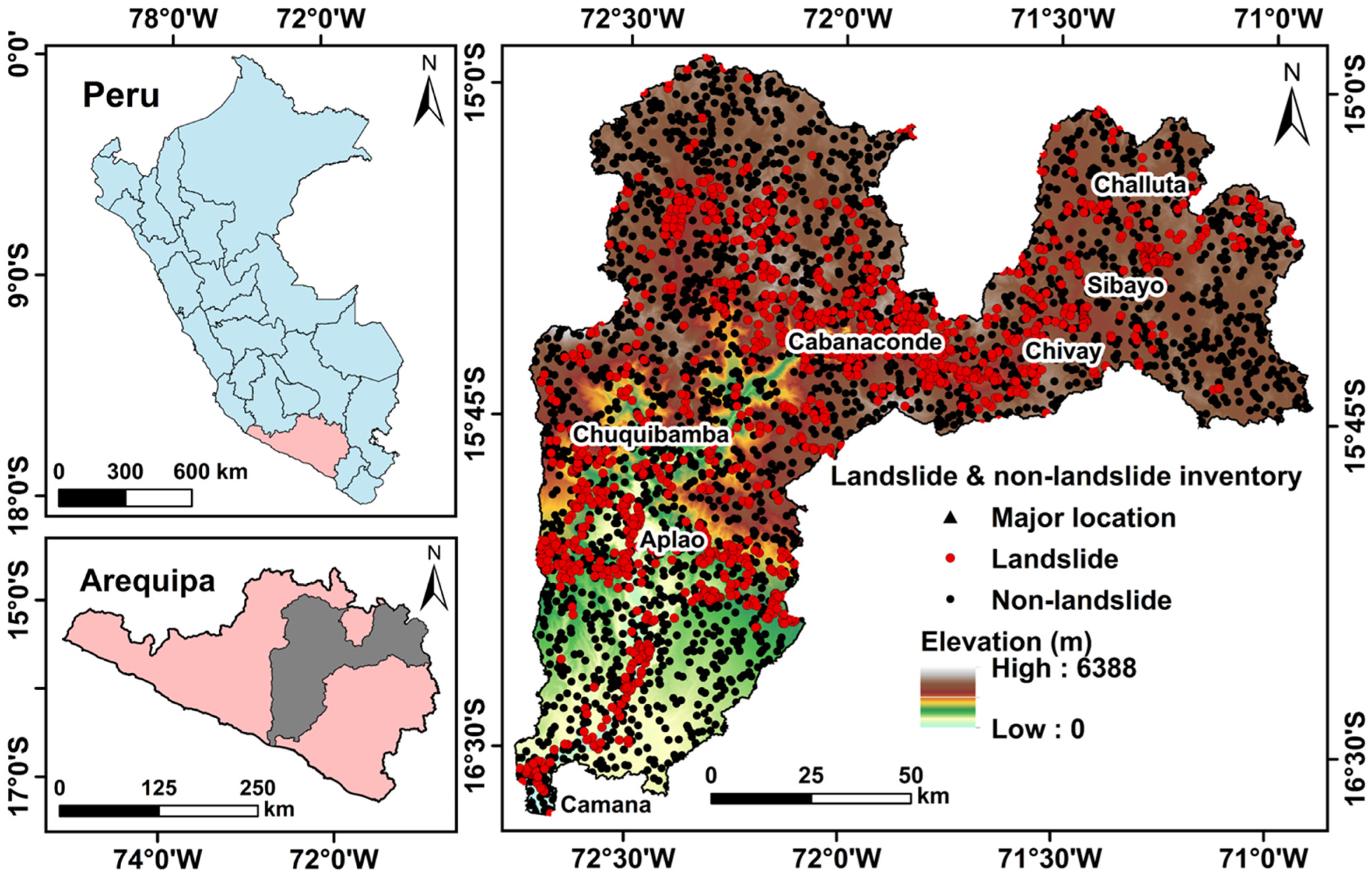
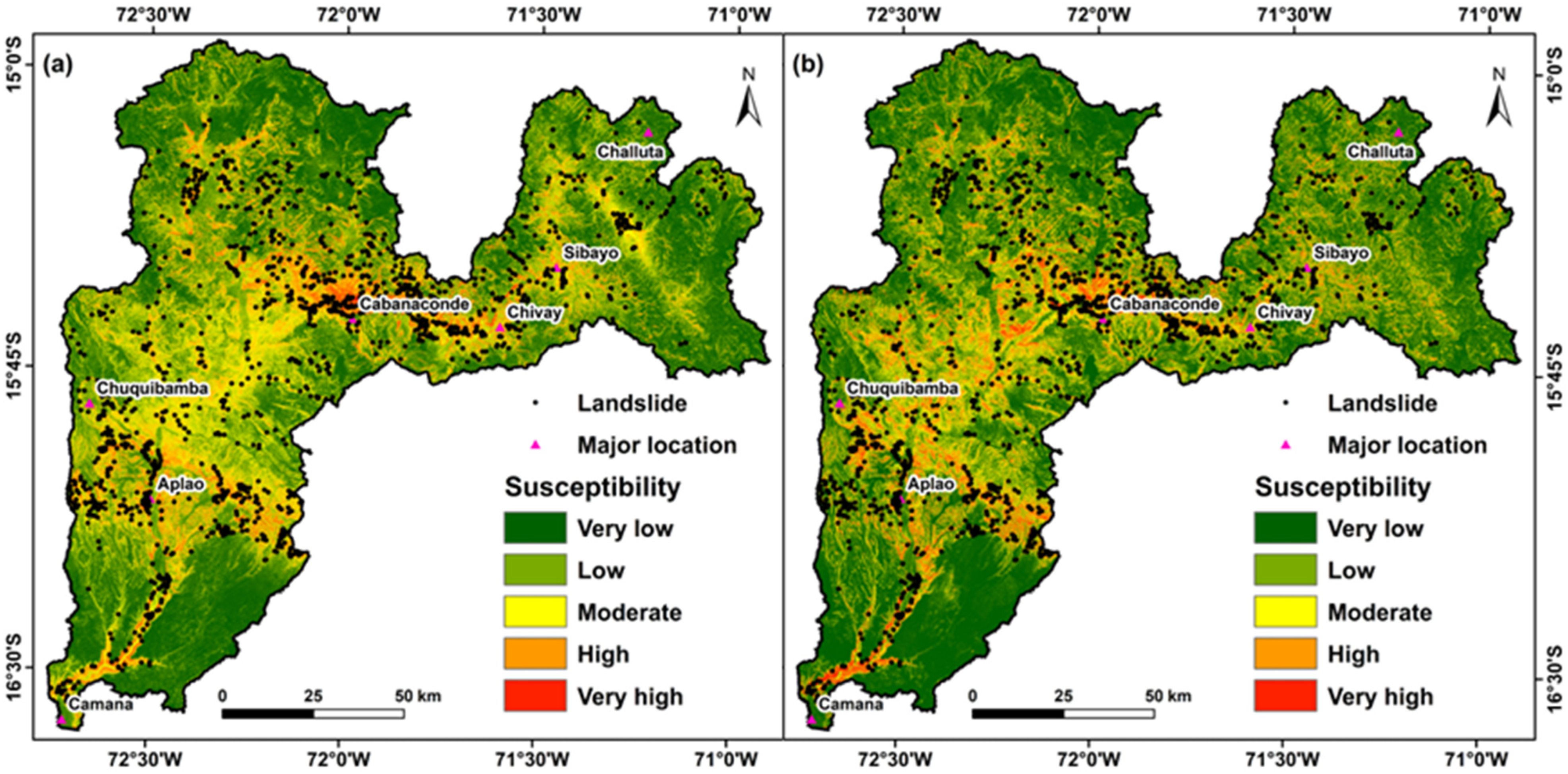
2.1. Study Area

The study area is in the Arequipa Region of southern Peru, covering a total area of 16,955 km². Geographically, the area is located between 72°45′29″W to 70°54′6″W longitude and 14°55′48″S to 16°39′29″S latitude. Figure 1 provides an overview of the study area and the geo-location of landslides. The area was selected for this study because of its high landslide vulnerability and the availability of suitable geospatial and auxiliary datasets at a regional scale. Cabanconde, Chivay, and Aplao are three populated locations in the area that are especially susceptible to landslides. The area is characterized by cold–arid climatic conditions, highly variable topography, and active seismicity. The average annual rainfall received in the area is approximately 95 mm/year, where most of the months are dry, except January to March. Cambisols, Regosols, and Leptosols are common soil types in the area. Regosols and Cambisols are predominantly found in the northern and southern regions, respectively, while Leptosols are commonly found across the region. Most of the study area is categorized as scrubland and barren land. The five major geological groups and formations of the area include the Puno group, Barroso group, Orcopampa formation, Moquegua formation, and Ichicollo formation. The geo-environmental setting of the area favors a diverse range of landslides, including rockfall, debris flows, and rotational and translational slides at different scales [8].

Figure 1. Geographical location and landslide training data wrapped over the DEM of the study area (adapted after the work of Kumar et al. [8]).

Kumar et al. [8] mapped areas of high to very-high landslide susceptibility concentrated in the central part of the study area. Most of these regions are characterized by steep slopes, barren land, and sparse vegetation cover, which leaves the soil exposed and vulnerable to slope failure. A higher association of landslides was observed with loose and unconsolidated sediments of the Ambo group, the Huaylillas formation, and the Camana formation. The major faults and proximity to historical earthquake epicenters are also associated with landslides in the area. These findings highlight the complex relationship of geo-environmental factors and landslide susceptibility in the area.

2.2. Datasets

High-resolution Google Earth imagery, local community knowledge, and field data were used to develop a landslide inventory database of the study area. A total of 1460 landslides were mapped in the area. The non-landslide locations were prepared in a GIS environment and used as training datasets for developing ML models. Twenty-four landslide influencing factors (LIFs) were derived from various data sources, including the Advanced Spaceborne Thermal Emission and Reflection Radiometer (ASTER) DEM; Landsat 8 reflectance data; thematic maps of geology, hydrogeology, geomorphology, land use/land cover, soil type, and average annual rainfall for ten years; earthquake epicenter location and magnitude; and road networks in the GIS environment. Table 1 briefly outlines the LIFs used in this study, along with references to previous studies supporting their inclusion in LSM.

Table 1. The LIFs prepared using geospatial and auxiliary datasets in the GIS environment [8].

LIF	Data and Resolution	References
Elevation	ASTER DEM (30 m)	[31,32]
Aspect		[12,33]
Slope		[34]
Profile curvature		[35]
Topographical position index (TPI)		[36]
Topographical roughness index (TRI)		[37]
Topographical wetness index (TWI)		[38]
Stream transportation index (STI)		[39]
Stream power index (SPI)		[40]
Surface relief ratio (SRR)		[41]
Stream/drainage density		[41]
Direct radiation		[7,42]
Direct duration radiation (DRR)
NDVI	Landsat 8 (30 m)	[43]
Geology	Reference maps (1:50,000)	[44,45]
Hydrogeology
Geomorphology
Land use/land cover	ESRI LULC map, 2020 (10 m)	[46]
Rainfall	Averaged GPM data (2010–2020) (10 km)	[47]
Soil type	Soil map (250 m)	[48]
Distance to major faults	Reference map (1:50,000)	[49]
Distance to major roads	Road network (2021)	[50]
Earthquake magnitude	USGS historical earthquake data (1973–2021)	[51,52]
Distance to epicenter

All LIFs were resampled to 30 m using the nearest neighbor resampling method in the GIS environment. The input variables are often measured in different units and have varying ranges, which can otherwise disproportionately influence the model’s results. To reduce this effect, we standardized the continuous variables by centering and scaling with the mean and standard deviation of the training datasets. The variance inflation factor of the LIFs was computed to test multicollinearity and found to be within an acceptable range (i.e., <10). To compute the relative importance of the LIFs, an ensemble feature selection method was developed using the Relief-F (v0.1.2) [53], gain ratio (v1.6.8) [54], and Chi-square (v1.1.1) [55] feature selection method in R (v4.4.2) [56]. The relative importance value was then used to order variables. For more details on the training data collection, preparation of LIFs, and development of ensemble feature selection used in this study, please refer to our previous work in Kumar et al. [8].

2.3. Methods

A workflow chart of the methodology used in assessing the impact of SAC on ML models’ performance in LSM is presented in Figure 2. The methods are discussed as cross-validation approaches, ML algorithms, computation of spatial autocorrelation, performance metrics, and learning curve analysis.

Figure 2. Workflow diagram of the methodology adopted in this study.

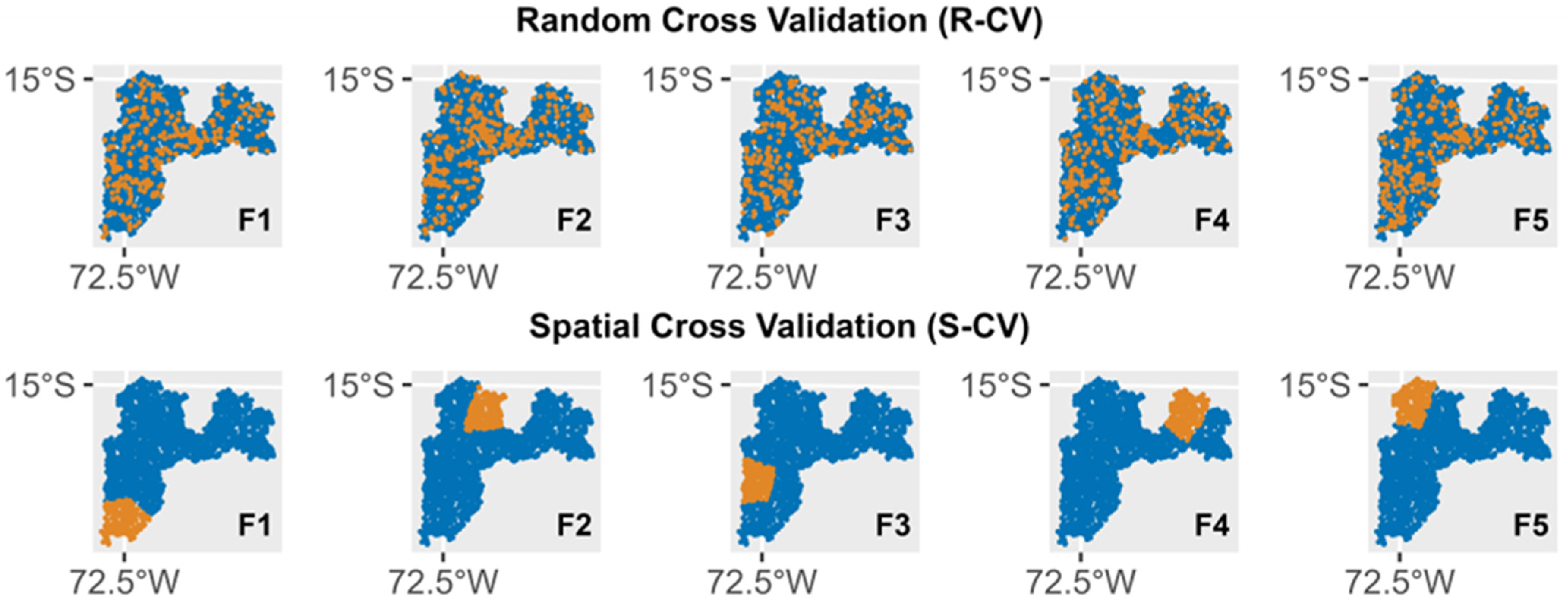
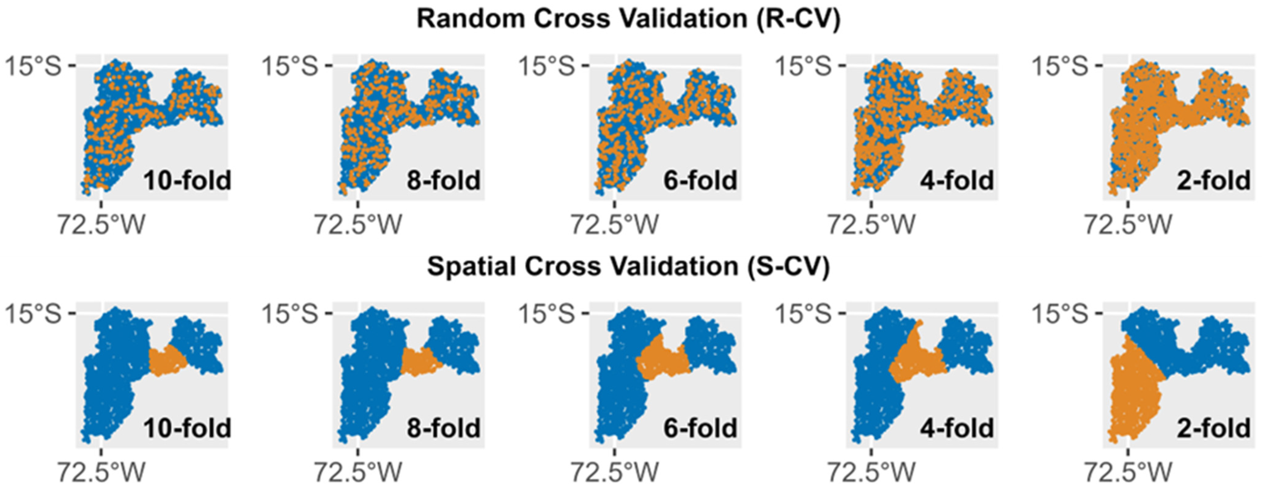
2.3.1. Cross-Validation Approaches

R-CV is commonly used in evaluating ML model performance where the entire dataset is split into training and testing subsets randomly, without considering the spatial dependency of the data. The S-CV is a modified version of the R-CV that employs k-means clustering on sample coordinates to obtain spatially independent training and testing datasets [19,25]. In both approaches, the training data iteratively consists of k-1 sets, while withholding a different set of testing data. The testing data are located relatively near to and far from the training data in the cases of R-CV and S-CV, respectively. We used 10-fold cross-validation with five repetitions for both methods. Figure 3 exhibits an example of the spatial distribution of the training and testing samples of the first 5 folds of 10-fold R-CV and S-CV methods.

Figure 3. Spatial distribution of training and testing samples of first 5 folds of 10-fold R-CV and S-CV methods. Blue and orange dots represent training and testing samples, and F represents fold numbers.

2.3.2. Machine Learning Algorithms

Table 2 summarizes the seven ML algorithms that were evaluated in this study: LDA, LR, k-nearest neighbor (KNN), ANN, SVM, RF, and C5.0 using the “mlr” package (v2.8) [57] in the R programming language. These algorithms were selected because they are widely used in LSM and represent a diverse range of model complexity. LDA, LR, and KNN are relatively simpler algorithms, while SVM, ANN, RF, and C5.0 are more complex [58,59,60,61]. The hyperparameter tuning of these models was performed using the grid search method.

Table 2. An outline of ML algorithms used in this study [8].

	Summary	Pros and Cons
LDA	It uses a dimensionality reduction technique to project higher feature spaces to a lower dimension of the input feature set for improved separation of classes [62]. The implemented LDA does not consist of tuning hyperparameters.	Pros: computationally efficient and interpretable. Cons: assumes a normal distribution of data and is sensitive to outliers.
LR	It utilizes the logistic function to learn the relationship between binary dependent and input variables. It is frequently used as a baseline model for comparing the effectiveness of other ML models. The implemented LR does not consist of tuning hyperparameters.	Pros: computational effectiveness and interpretable. Cons: requires a large sample size, assumes linearity among dependent and independent variables.
KNN	It performs classification and regression tasks on new data by measuring the similarity [5]. k is a tuning hyperparameter in implemented KNN, which implies the number of nearest samples.	Pros: non-parametric and computationally efficient. Cons: sensitive to noise and irrelevant variables.
SVM	It uses a hyperplane to separate two classes accurately [63]. The developed SVM has two hyperparameters: cost and gamma, controlling the penalty for wrongly classified samples and the complexity of the hyperplane.	Pros: effective in high-dimensional feature spaces, generalization, and availability of various kernel functions. Cons: computationally intensive and lack of interpretability.
ANN	A typical ANN architecture consists of an input, hidden, and output layer. It uses mathematical transformation to find patterns of input data [64]. Size and decay are two hyperparameters of implemented ANN, which implies the number of nodes in the hidden layer and the regularization term.	Pros: features learning, scalability, and ability to learn complex patterns. Cons: computational complexity, huge training data requirements, and lack of interpretability.
RF	It consists of many decision trees. RF uses the bagging method to obtain accurate results by generating a random training set with the replacement [65]. The used RF model consists of one hyperparameter, i.e., the number of input variables (mtry) at each split of the decision trees.	Pros: efficient in high-dimensional feature handling, robustness to outliers, and inbuilt feature selection. Cons: memory and computationally intensive.
C5.0	It uses boosting and weighing approaches to develop decision trees to improve the model’s accuracy [66]. The developed C5.0 model has one hyperparameter: trials. This is also known as boosting iterations, which control how many models are used in the final model.	Pros: ability to handle mixed data types, robustness to noise, and inbuilt feature selection. Cons: large training data requirement, sensitive to outliers, and can potentially overfit if a complex model is developed.

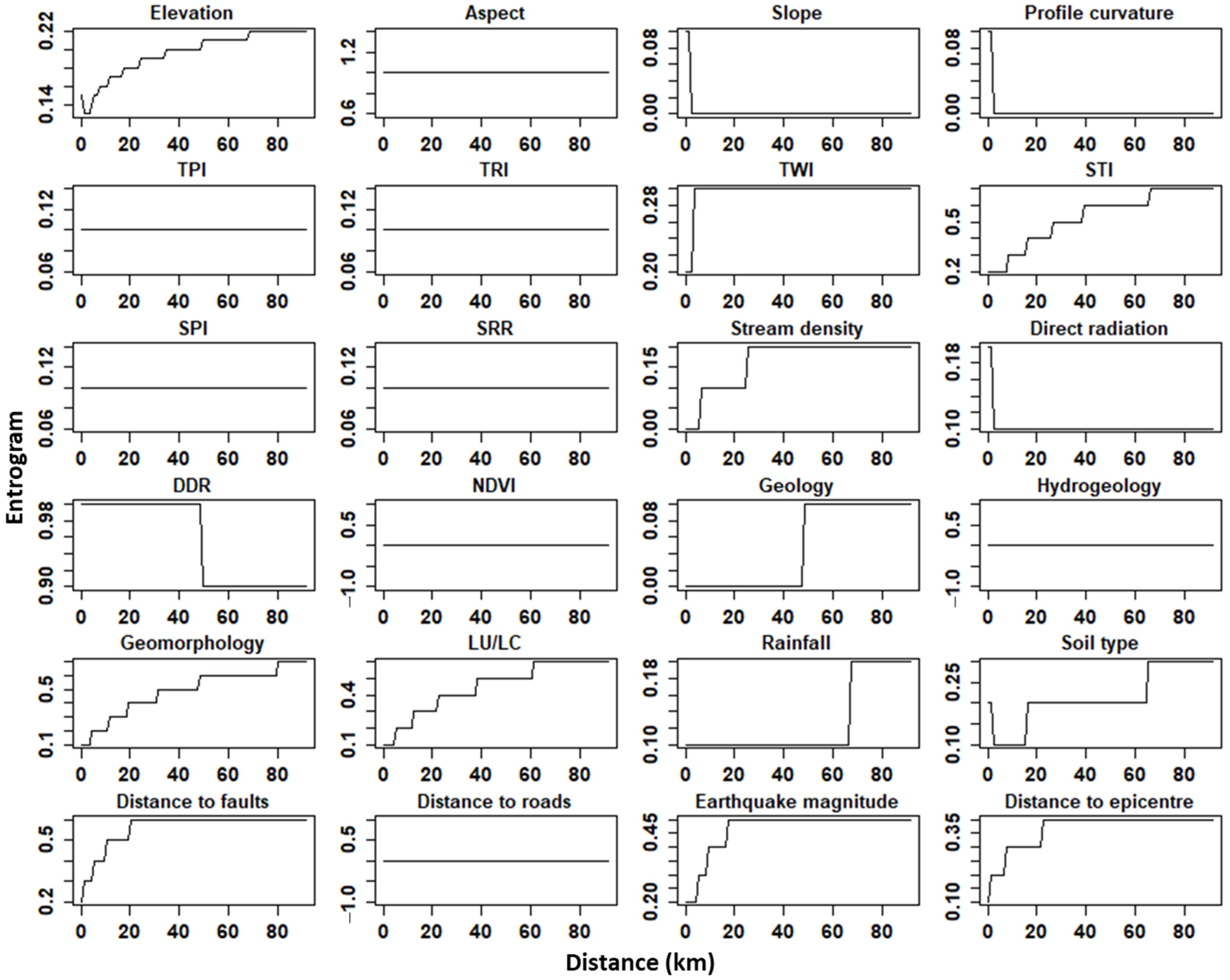
2.3.3. Computation of SAC

Spatial datasets often show spatial dependency, where the values of a variable at nearby locations are similar to those at distant locations. In this study, we used an entrogram to measure the global SAC of each variable within the study area. The entrogram for each variable is developed based on an entropy-based local indicator of spatial association (ELSA) [67]. We used the ELSA package (v1.1-28) in R to derive the entrogram of each variable. The advantage of using ELSA over other techniques (such as variograms) is that ELSA can be applied to both categorical and continuous variables of different types, including points, polygons, and raster layers. ELSA at location i can be calculated using Equation (1).

$$E_i=E_{ai}\times E_{ci}$$

(1)

$E_{ai}$ describes the feature dissimilarity between location i and the adjacent locations. $E_{ci}$ describes the diversity of the classes of a variable within the local distance from location i. The value $E_i$ ranges from 0 to 1, where lower and higher values represent higher and lower SAC, respectively. Detailed documentation of ELSA is provided by Naimi et al. [67].

2.3.4. Performance Metrics

We used the area under the receiver operative characteristic (ROC) curve (AUC) as a primary metric to evaluate the ML models’ performance, as it has been widely used in LSM [27,68]. AUC assesses the model’s overall ability to correctly classify landslide and non-landslide areas across all possible thresholds. AUC is calculated by estimating the total area under the ROC curve using Equation (2).

$$AUC={\displaystyle \frac{\sum TP+\sum TN}{TP+FP+TN+FN}}$$

(2)

where $TP$: true positive, $TN$: true negative, $FP$: false positive, and $FN$: false negative. AUC value ranges from 0–1, where ≤0.5 corresponds to a random classifier, ≥0.7 is generally considered acceptable, ≥0.8 is excellent, and ≥0.9 is outstanding [68]. Along with AUC, the overall accuracy (the proportion of correctly classified landslide and non-landslide samples) and recall (the proportion of correctly classified landslide samples) were also computed to evaluate model performance.

2.3.5. Learning Curve Analysis

A learning curve analysis was performed to assess the impact of a number of variables and training data quantity on model performance in the context of the two CV methods considered. We based this analysis on the rank of the input variables derived from Kumar et al. [8]. We used the top five variables and incrementally incorporated the next five variables (i.e., 5, 10, 15, 20, and 24) and measured the performance statistics using both CV methods considered. Furthermore, we used varying training data quantities (ranging from 10% to 100%) and measured their performance statistics to assess their impact on model performance.

3. Results

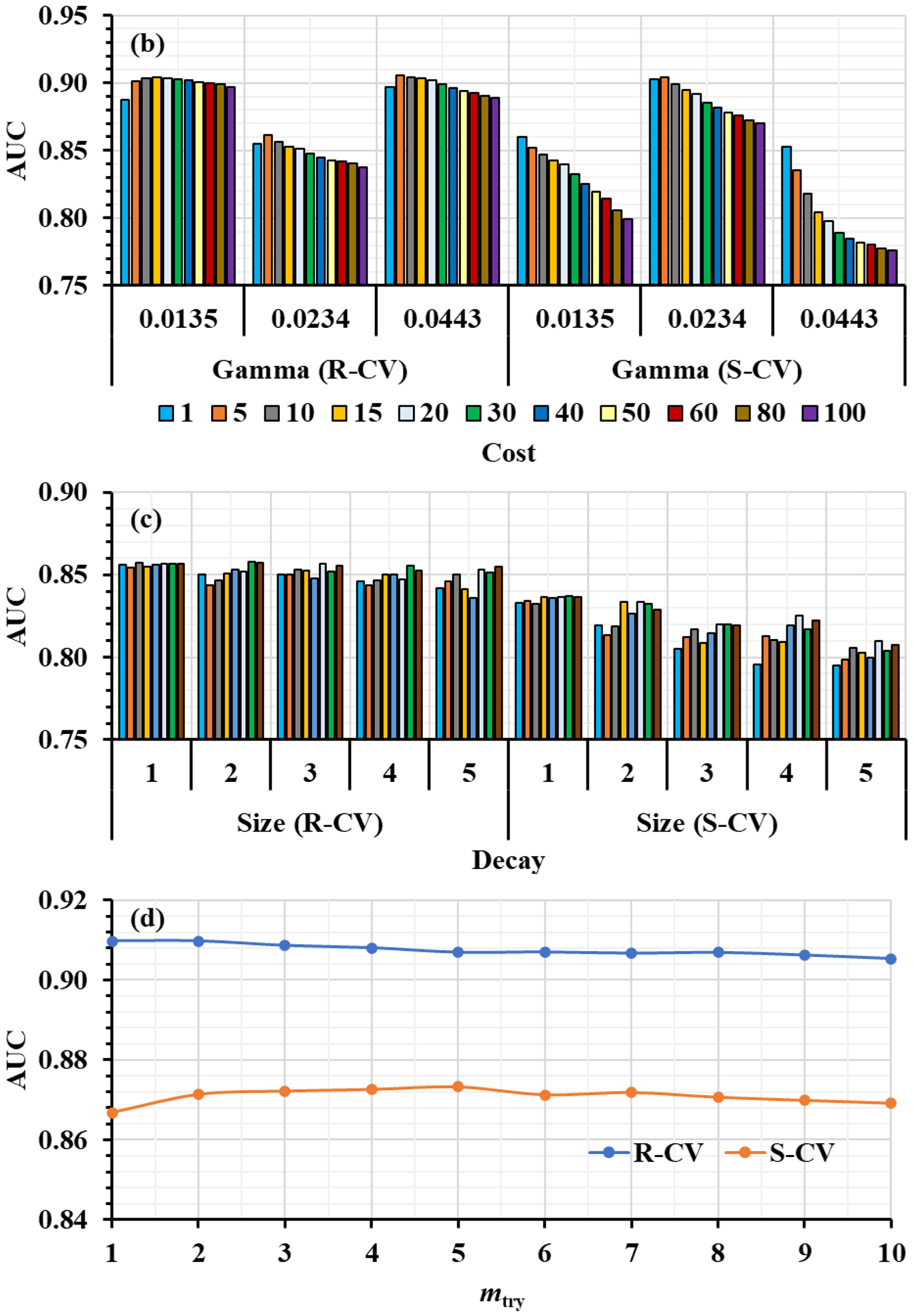
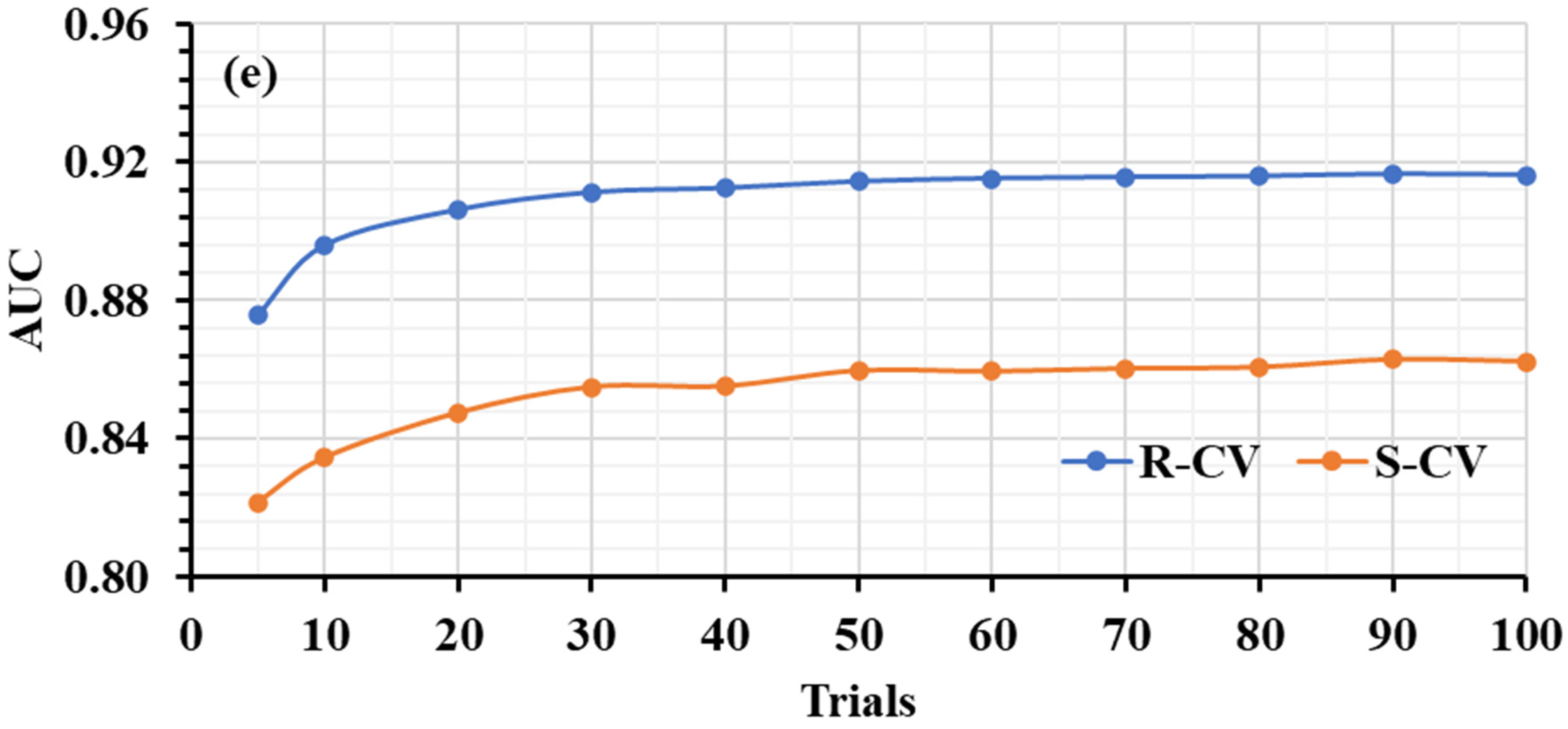
3.1. Hyperparameter Tuning

The search spaces and optimal values of the hyperparameters of different ML models are given in Table 3. The LDA and LR have not been included in this section, as these models do not require hyperparameter tuning. Figure 4a–e displays the AUC of the ML models across different hyperparameter values obtained using R-CV and S-CV. Figure 4a shows the AUC values of KNN using R-CV and S-CV. The R-CV identified a smaller k (i.e., 27) whereas S-CV preferred a large k value (i.e., 241) to achieve optimal performance in predicting landslide and non-landslide areas. For the SVM, R-CV and S-CV identified 0.0234 and 0.0135 as optimal gamma values, respectively, and the same cost value (i.e., 5) to achieve the best result (Figure 4b). For ANN, the R-CV and S-CV identified the same size and decay values (i.e., 1 and 0.01, respectively) as optimal to obtain maximum accuracy (Figure 4c). For the RF, the optimal value of m_try was identified as 1 and 5 using R-CV and S-CV, respectively (Figure 4c). However, it should be noted that the RF did not show a noticeable impact of m_try on model accuracy, irrespective of the CV methods used in the performance assessment. R-CV and S-CV identified the same number of trials (i.e., 90) as optimal for C 5.0 (Figure 4e).

Table 3. The optimal values of different hyperparameters of ML models derived using R-CV and S-CV methods. The LDA and LR are not included, as they do not consist of any tuning hyperparameters.

	R-CV	S-CV	Grid Search Space
KNN	k = 27	k = 241	k = 3, 5, 7, 9, 11, 13, 17, 21, 27, 31, 33, 41, 49, 55, 61, 69, 79, 99, 111, 119, 129, 139, 149, 169, 189, 211, 229, 241, 259, 279, 301, 331, 351.
SVM	cost = 5 gamma = 0.0443	cost = 5 gamma = 0.0234	cost = 1, 5, 10, 15, 20, 30, 40, 50, 60, 80, 100; gamma = 0.0135, 0.0234, 0.0443.
ANN	size = 1 decay = 0.01	size = 1 decay = 0.01	size = 1, 2, 3, 4, 5; decay = 0.0001, 0.00024, 0.00056, 0.0014, 0.0032, 0.0050, 0.0075, 0.01.
RF	mtry = 1	mtry = 5	mtry = 1, 2, 3, 4, 5, 6, 7, 8, 9, 10.
C5.0	trials = 90	trials = 90	trials = 5, 10, 20, 30, 40, 50, 60, 70, 80, 90, 100.

Figure 4. Hyperparameter tuning of different ML models using R-CV and S-CV configurations. (a) KNN, (b) SVM, (c) ANN, (d) RF, and (e) C5.0.

R-CV and S-CV showed differing degrees of the sensitivity of ML performance to the selected hyperparameter values, particularly for the SVM and ANN models. For SVM, R-CV tuning implies that gamma is a more crucial hyperparameter than cost, whereas S-CV indicated both as crucial hyperparameters in obtaining accurate results. Similarly, based on the R-CV tuning of ANN, one would have an impression that decay is relatively more important than size, whereas S-CV indicates that both are crucial hyperparameters for obtaining accurate results. It is worth noting that in all the ML models, R-CV-based hyperparameter selection produced noticeably higher AUC values than did S-CV, indicating an overly optimistic performance estimation. The RF model demonstrated the least sensitivity to the hyperparameters as compared to other ML models (irrespective of the CV methods considered).

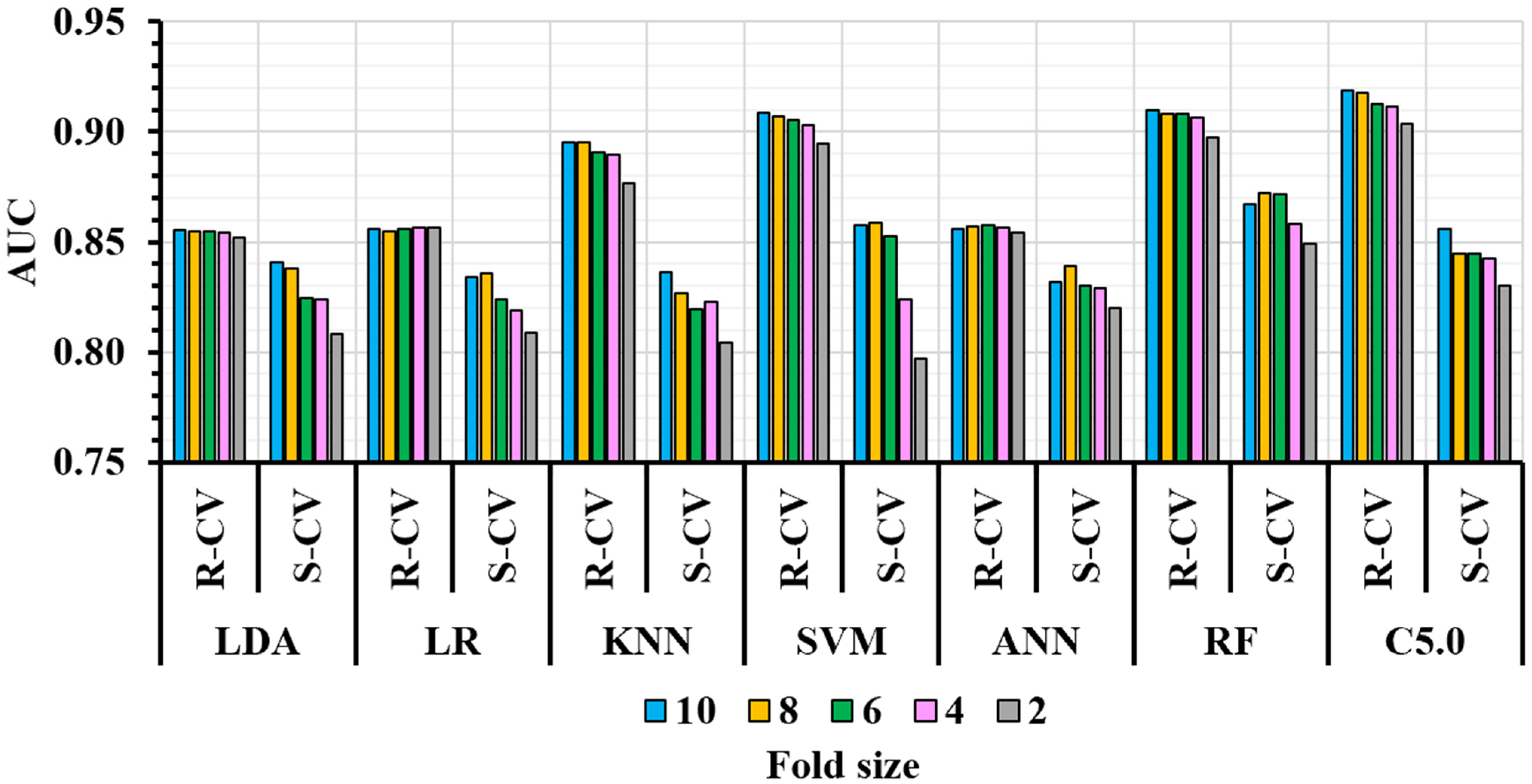
3.2. ML Performance Assessment

ML models with optimal hyperparameter settings were tested to assess their performance using R-CV and S-CV methods (Figure 5 and Table 4). The R-CV-based performance assessment of all implemented ML models resulted in significantly higher accuracy, as expected due to relatively similar training and testing data, as compared with S-CV. Moreover, the discrepancy between the performance metrics estimated using both CV methods of ANN, LDA, and LR was less when compared to that of other ML models. S-CV-based assessment of ML models also indicates a higher variability in their performance when compared with that of R-CV, indicating a noticeable spatial variability in model performance across different geographic regions that was not captured by R-CV. A higher spatial variability of ML models indicates poor generalization ability across different geographic regions. It is interesting to note that despite being simple models, LDA and LR show comparable generalization ability (i.e., S-CV results) as that achieved using sophisticated ML models. The RF, C5.0, and SVM slightly outperformed other models, including LDA, KNN, LR, and ANN, in both CV methods (Table 4). Figure 6 displays the variability in the susceptibility maps generated using two models: C5.0, which showed a larger discrepancy between R-CV and S-CV performance, and ANN, which exhibited a smaller difference. This variation highlights how SAC can influence model assessment. The lower discrepancy between R-CV and S-CV generally indicates better model generalization, as evidenced by the lower variance in the AUC values observed for the ANN model.

Figure 5. AUC values of ML models using R-CV and S-CV configurations.

Table 4. AUC, overall accuracy (OA), and recall of different ML models using R-CV and S-CV configurations.

	LDA		LR		KNN		SVM		ANN		RF		C5.0
	R-CV	S-CV	R-CV	S-CV	R-CV	S-CV	R-CV	S-CV	R-CV	S-CV	R-CV	S-CV	R-CV	S-CV
AUC	0.86	0.84	0.86	0.83	0.89	0.84	0.91	0.86	0.86	0.83	0.91	0.87	0.92	0.86
OA	0.78	0.77	0.79	0.77	0.80	0.76	0.82	0.79	0.79	0.77	0.82	0.79	0.83	0.77
Recall	0.69	0.63	0.71	0.65	0.77	0.66	0.78	0.68	0.76	0.70	0.78	0.66	0.81	0.63

Figure 6. Landslide susceptibility maps of the study area obtained from (a) C5.0 and (b) ANN models.

We further evaluated the performance of ML models across different fold sizes (i.e., 10, 8, 6, 4, and 2) using both R-CV and S-CV. As illustrated in Figure 7, smaller fold sizes increase the proportion of testing data. Crucially, under S-CV, smaller folds also increase the average spatial distance between the training and testing data, creating more spatially independent partitions for a rigorous assessment of model generalization.

Figure 7. A pictorial representation of different fold sizes and their impact on the proportion of training and testing data partitions using R-CV and S-CV configurations. Blue and orange dots represent training and testing samples, respectively.

Our analysis revealed a key difference between the two methods: R-CV produced similar performance estimates, regardless of fold size, while S-CV showed a performance reduction, as the fold size decreased from 10 to 2 (Figure 8 and Table S1). This decline in S-CV performance likely stems from the increasing discrepancies in geographic conditions between the training and testing sets at smaller fold sizes.

Figure 8. Impact of fold size on ML models’ performance using R-CV and S-CV.

These results imply that R-CV can lead to over-optimistic performance estimates, potentially misleadingly suggesting accurate predictions, even beyond the training data’s spatial extent. Notably, ANN exhibited the least variability in S-CV performance across different fold sizes, indicating superior generalization across diverse geographic regions. The fold size or distance between the training and testing sets should be chosen carefully to obtain reliable performance estimation. A balance should be struck between achieving spatially independent partitions and maintaining sufficient training data for robust model learning.

3.3. Learning Curve Analysis

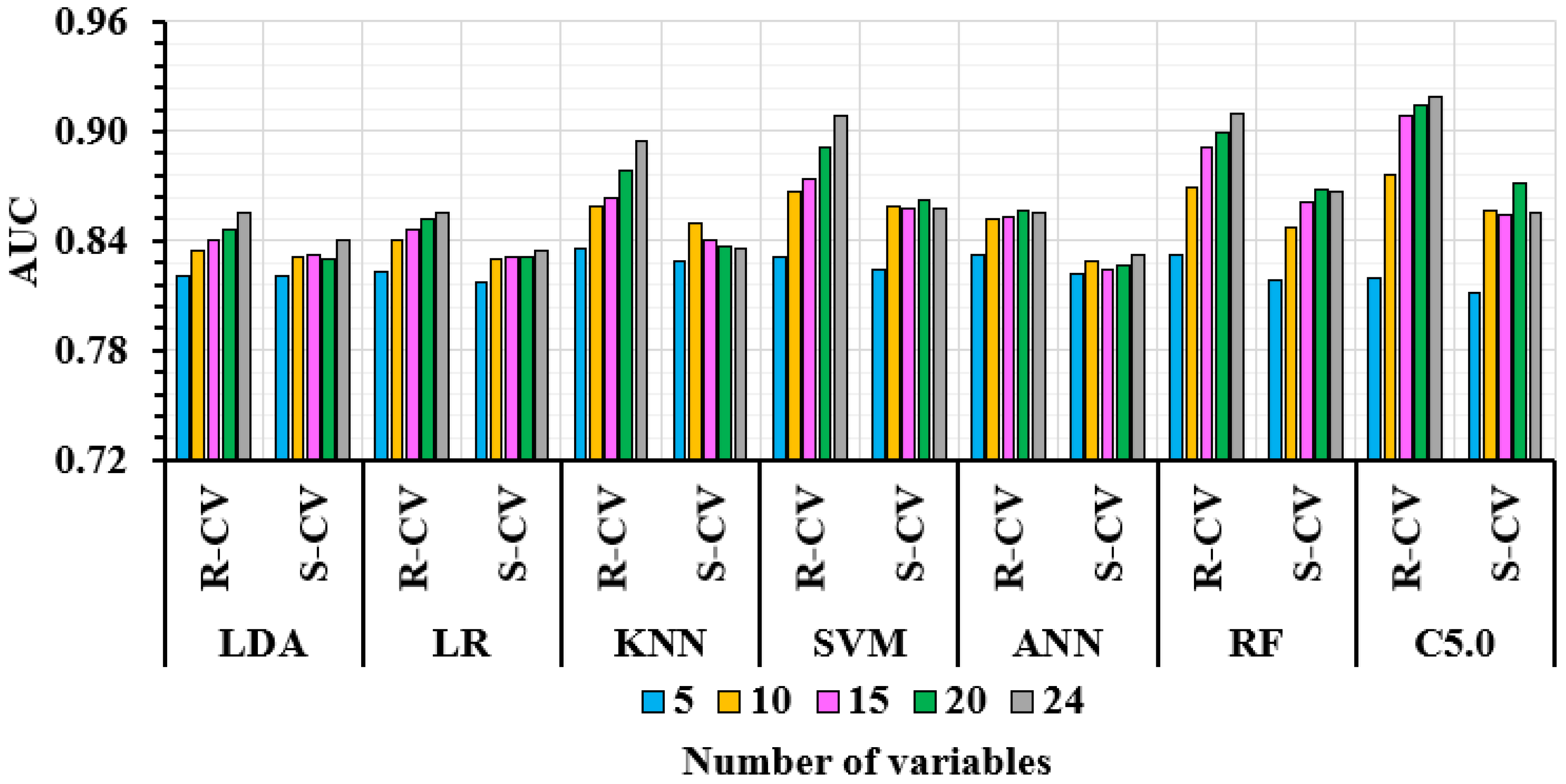
3.3.1. Number of Variables and ML Performance

The impact of the number of variables on ML models’ performance was assessed using R-CV and S-CV methods. Figure 9 and Table S1 display the performance statistics of ML models using different numbers of variables based on R-CV and S-CV methods. These variables were sorted based on their relative importance, measured using the ensemble feature selection method [8]. The R-CV-based performance assessment of the ML models produced a noticeably higher AUC value as the number of variables increased, whereas S-CV, except for the RF and C5.0 models, did not indicate this. The R-CV and S-CV exhibit the least discrepancy in ML performance assessment when using only five variables, but the discrepancy increases noticeably as the number of variables increases from 5 to 15 or higher. This suggests that training using the R-CV approach is more likely to produce an overfitted ML model. Our results provide important context for the selection of important variables using wrapper feature selection methods, as these rely on the ML model for ranking the relative importance of the variables. A wrapper feature selection method using R-CV, as commonly used in geospatial applications, could produce a biased or optimistic number of variables, as SAC gets ignored while partitioning training and testing subsets.

Figure 9. Impact of the number of variables on ML performance assessed using R-CV and S-CV.

The ANN indicated strong performance using both CV approaches and demonstrated the least sensitivity to the number of variables when compared with the results for other ML models. The LDA and LR showed a moderate change in their performance as the number of variables increased from 5 to 24 using both CVs. The R-CV-based performance assessment of KNN and SVM indicates a substantial increase in their AUC values as the number of variables increases, whereas the S-CV-based assessment does not. The RF improves its AUC values as the number of variables increases, irrespective of the CV methods used in the performance assessment. Considering these results together, it is clear that the impact of SAC in spatial predictive modeling increases as the number of variables rises, resulting in optimistic model performance estimation. Moreover, the most complex models (including SVM, RF, and C5.0), with the exception of the ANN, are more prone to produce optimistic results than are simpler models like LDA and LR, with the exception of KNN.

The number of variables and the severity of potential predictive performance overestimation obtained using R-CV are also related to the SAC of the individual variables. Figure 10 shows the entrogram of the different LIFs used in this study. Lower and higher entrogram values indicate higher and lower SAC, respectively. Most of the LIFs show low entrogram values, indicating a high degree of SAC. ML models developed using LIFs with high SAC are expected to show higher discrepancies between accuracy assessed using R-CV and S-CV. LIFs, including elevation, TWI, STI, geomorphology, distance to major faults, LU/LC, distance to epicenter, and earthquake magnitude, show a substantial decrease in SAC as the distance increases. This implies that samples collected beyond a certain distance can potentially reduce the SAC and hence, their impact on model performance can be minimized. Aspect and DDR are two LIFs for which their entrogram value is close to 1, indicating negligible SAC. Interestingly, the discrepancy between the AUC values derived from R-CV and S-CV is more pronounced in ML models developed using a greater number of variables as opposed to those developed using fewer variables, as illustrated in Figure 8. This can be attributed to the inherent SAC of LIFs, for which a greater number of variables amplifies the total influence of SAC on the model. Effectively, model complexity increases as the number of variables rises, potentially resulting in overfitting and poor generalization ability. While this phenomenon is well-documented in general [69,70], it has not been previously well-explored in the context of spatial models for regional landslide susceptibility assessment.

Figure 10. Entrogram of different LIFs showing the SAC.

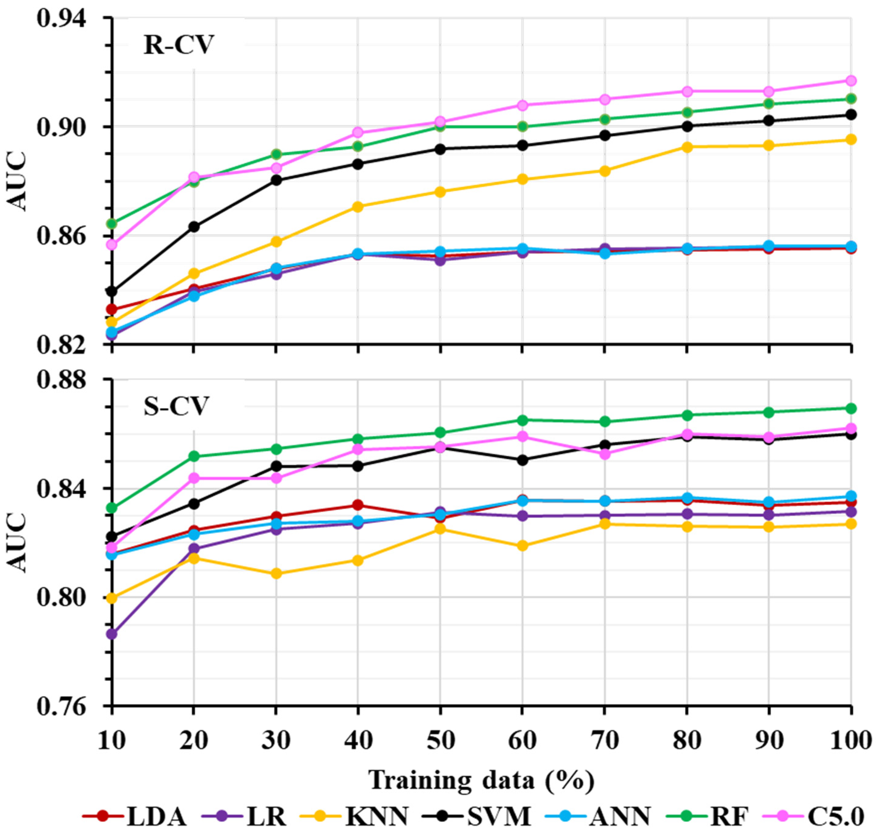
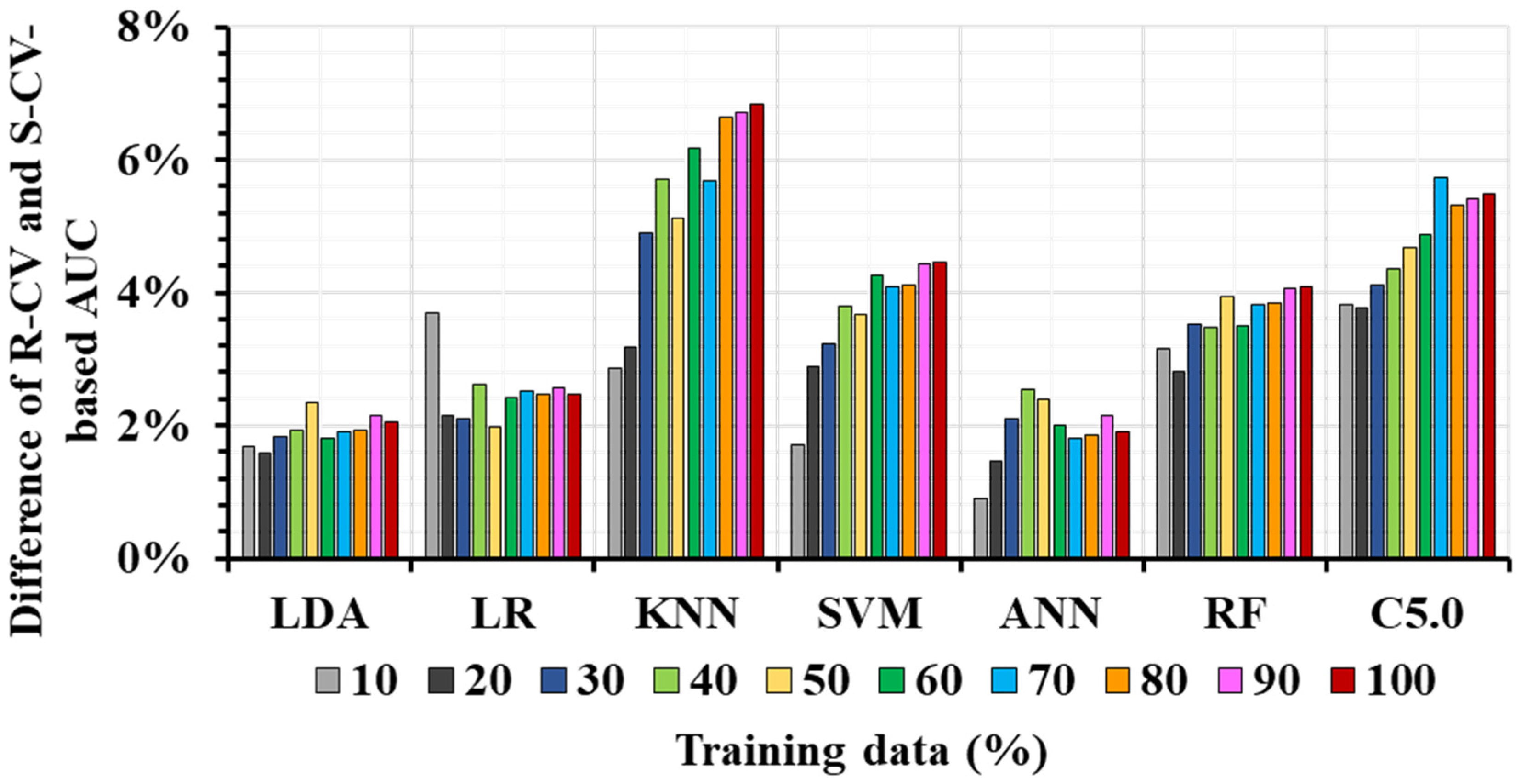
3.3.2. Training Data Quantity and ML Performance

We assessed the impact of training data quantity on ML performance with respect to the R-CV and S-CV methods. Unlike the fold assessment experiment, in which the total sample size remains constant, but the proportion of training and testing data varies (see Section 3.2), this experiment involves a change in the total sample size. Figure 11 and Table S3 present the performance statistics of different ML models of varied training data quantity (ranging from 10% to 100%), computed using both the R-CV and S-CV approaches. The experimental results demonstrate that the impact of training data quantity on model performance was more profound when assessed using R-CV than S-CV. This impact was larger for complex models like SVM, RF, and C5.0 (except ANN) than for simple models like LDA and LR (except KNN). Figure 12 shows the difference in AUC values calculated from the R-CV and S-CV of different ML models. As an example, the R-CV-based AUC value of KNN increases from 0.83 to 0.90 as the training data increases from 10 to 100%, but the S-CV only shows a nominal increase in AUC values (i.e., 0.80 to 0.83). Similarly, the R-CV-based AUC value of C5.0 increases from 0.86 to 0.92 as the training data increases from 10 to 100%, while the S-CV-based AUC value increases from 0.82 to 0.86. Similar trends were seen for SVM and RF as well. In general, the R-CV-based assessment of model performance portrays a significant improvement in model performance as the training data increases. The optimistic outcomes stemming from the R-CV-based performance estimation can mislead perceptions about the influence of the training data quantity for optimal model performance. The satisfactory accuracy statistics of all ML models using just 10% of the total training samples in the S-CV case indicates that a small amount of spatially diverse data is more valuable than a large amount of spatially concentrated data.

Figure 11. Impact of training data quantity on ML models’ performance using R-CV and S-CV.

Figure 12. Differences in R-CV and S-CV-based AUC resulting from varying training data quantity.

4. Discussion

4.1. Hyperparameter Tuning

Hyperparameter tuning is one of the most crucial steps in the successful implementation of ML methods, as the default values cannot ensure the best possible outcome from these models [71]. However, the magnitude of improvement associated with hyperparameter tuning usually depends on the sensitivity of the hyperparameter(s) to the model’s performance and the characteristics of the input data. There is also a possibility that both R-CV and S-CV may produce the same or different hyperparameter values, with noticeable to minimal or no effects on the model’s performance [26]. For example, the RF does not show a noticeable improvement in its performance after performing hyperparameter tuning (with either CV method). On the other hand, the SVM performance shows considerable sensitivity to hyperparameter tuning, but only in the S-CV case. The discrepancy between the importance of the hyperparameters assessed using both the alternative CV methods is interpreted to depend on the SAC inherent in the input data.

The major challenge in hyperparameter tuning is that there are no universal optimal search spaces for finding optimal values. The user needs to explore a large enough search space to find a global solution. If hyperparameter values are distributed at the margin, it suggests that the optimal values may lie outside of the search space [26]. To overcome this issue, we used a random search method to find the possible ideal search space and then adopted a grid search approach to obtain the optimal hyperparameter of different ML models. The final decision for selecting the hyperparameter values should be made carefully by incorporating domain knowledge to reduce the model’s complexity and overfitting. For example, a higher m_try value of the RF would increase the model complexity relative to that of an RF developed using a lower m_try value. Higher cost and gamma values for SVM correspond to a more complex hyperplane. For KNN, lower and higher k values may result in relatively noisy and smooth decision boundaries, respectively. For ANN, higher and lower decay values may cause the model to converge rapidly and be trapped, without finding an optimal solution. For C5.0, a large number of trials could result in the development of a complex ensemble model that may potentially overfit training data and be computationally demanding.

A comparison of CV methods, as presented in this study, is vital in evaluating a given ML model’s potential to overfit by iteratively testing its performance using held-out samples at each iteration. However, independence between training and testing data is key to estimating the biased-reduced performance of ML models [19]. In all ML models, the R-CV produced an overly optimistic performance improvement based on hyperparameter tuning (i.e., ~5–8% greater than those estimated using the S-CV method).

4.2. ML Performance and SAC

The biased-reduced performance assessment of ML models is important to evaluate their potential performance in practical (i.e., predictive) application scenarios. Results derived in this study show that R-CV often produces optimistic performance estimates for ML models due to ignoring the SAC inherent in spatial datasets (Figure 5 and Table 4). Our findings corroborate previous research comparing R-CV and S-CV methods for evaluating ML performance in diverse applications, including soil water permeability modeling [25], species occurrence prediction [19], ecological modeling [24], and apartment price modeling [30]. R-CV may still produce fair error estimates when the models are trained and evaluated in a small geographic region [19]. Consequently, the performance estimates obtained using R-CV and S-CV tend to converge when evaluating models within the same feature spaces in which they were trained. However, if the goal is to evaluate the model’s ability to make predictions under diverse and new geographic conditions, S-CV is likely to produce more reliable performance estimates than R-CV. Higher variability in the boxplots of ML performance obtained using S-CV (Figure 5) stems from the relatively greater spatial heterogeneity between the training and testing partitions compared to those obtained using R-CV. This suggests that the elevated S-CV variability likely reflects the fact that different spatial regions of the training and testing data capture the overall domain trends to varying degrees.

The bias in R-CV primarily occurs due to the SAC of the input variables. The entrogram used in this study indicated that a few variables show a weak SAC beyond a certain distance. The SAC of the input variables to distance needs to be considered carefully when designing the fold size to obtain independent training and testing subsets. We assessed the models’ generalization ability using different fold sizes (i.e., 10, 8, 6, 4, and 2), which allowed for the consideration of varying degrees of independence between the training and testing sets. All the ML models showed a strong generalization ability, even after partitioning the entire region into only two folds. This could be due to the training data quality and the selection of suitable LIFs used in developing the ML models. S-CV-based performance assessment not only produces more reliable performance estimates than R-CV but also offers a deeper insight into ML performance across varying geographic conditions. By analyzing the regions in which the models fail to make accurate predictions, we can gain valuable insights into the potential causes of their poor performance. This information is crucial for designing robust sampling strategies that can effectively utilize the true potential of ML-based predictive modeling. Among all the models, the ANN produced the most stable prediction accuracy. The RF and C5.0 showed a noticeable increase in model accuracy as the number of variables increased for the R-CV case, as also found by Kumar et al. [8] for random training–testing data partitioning.

4.3. Limitations

Although S-CV accounts for SAC, it may also unknowingly induce extrapolation issues if the training and testing data partitions span feature spaces that are substantially different than intended. In such a scenario, the model needs to predict conditions outside the feature space included in training and may produce an unreliable model performance assessment [19]. Furthermore, S-CV should be used carefully to account for the spatial distribution of the samples. When data are poorly distributed or scarce, the S-CV approach may not be suitable, as the training and testing folds may not have sufficiently similar geo-environmental settings. Similar issues may arise, even when data are numerous but are clustered in a specific region of the study area. S-CV may also not be feasible when data are highly imbalanced, and classes are clustered in different geographic regions. Care should also be taken in designing fold size, and its influence on overall model performance should be interpreted carefully. S-CV should be chosen when the samples are spatially distributed for reliable assessment of the model’s performance and its ability to generalize to new locations. It is worth clarifying that we do not intend to invalidate the contribution made using the R-CV method but rather to draw researchers’ attention to the consequences of ignoring SAC in spatial predictive modeling. R-CV can still be a useful tool for quickly assessing the performance of a model, but it is important to be aware of its limitations.

5. Conclusions

Machine learning (ML) has been extensively used in spatial modeling, including landslide susceptibility prediction. The effectiveness of ML models is evaluated based on their performance statistics derived from training–testing data partitions. In this study, we demonstrated the implications of applying spatial cross-validation (S-CV) relative to the commonly used random cross-validation (R-CV) in the context of regional landslide susceptibility prediction. We assessed the impact of spatial autocorrelation (SAC), which is commonly ignored, on three crucial stages of ML modeling: hyperparameter tuning, performance evaluation, and learning curve analysis.

We considered seven ML models: logistic regression (LR), linear discriminant analysis (LDA), k-nearest neighbor (KNN), artificial neural network (ANN), support vector machine (SVM), random forest (RF), and C5.0. The experimental results showed that hyperparameter tuning performed using R-CV produced optimistic performance estimates compared to the hyperparameter tuning performed using S-CV (5–10% difference between optimized R-CV and S-CV results). R-CV also occasionally failed to reveal the true influence of the hyperparameters on model performance, as seen in the SVM and ANN models, specifically.

Overall, complex models such as RF, SVM, and C5.0 (except ANN) generally showed greater discrepancies between the R-CV and S-CV results compared to the results for simpler models such as LR and LDA (except KNN). R-CV showed notable performance improvements with increasing features and training data, particularly for complex models (again, except for ANN). Conversely, S-CV performance was substantially less influenced by the number of features or the training data volume for all ML models considered.

Our findings demonstrate the significance of considering SAC in conjunction with careful variable selection to improve model performance. R-CV, by ignoring SAC during data partitioning, can lead to optimistic performance estimates and poor generalization scenarios. Therefore, we recommend S-CV over R-CV for the reliable assessment of ML model performance in spatial predictive modeling.

References

- Highland, L.M.; Bobrowsky, P. The Landslide Handbook—A Guide to Understanding Landslides; U.S. Geological Survey: Reston, VA, USA, 2008.
- EM-DAT, C. Em-Dat: The Ofda/Cred International Disaster Database; Centre for Research on the Epidemiology of Disasters, Universidad Católic a de Lovaina: Ottignies-Louvain-la-Neuve, Belgium, 2020. [Google Scholar]
- Keefer, D.K.; Larsen, M.C. Assessing landslide hazards. Science 2007, 316, 1136–1138. [Google Scholar] [CrossRef] [PubMed]
- Chen, W.; Zhang, S.; Li, R.; Shahabi, H. Performance evaluation of the GIS-based data mining techniques of best-first decision tree, random forest, and naïve Bayes tree for landslide susceptibility modeling. Sci. Total Environ. 2018, 644, 1006–1018. [Google Scholar] [PubMed]
- Adnan, M.S.G.; Rahman, M.S.; Ahmed, N.; Ahmed, B.; Rabbi, M.F.; Rahman, R.M. Improving spatial agreement in machine learning-based landslide susceptibility mapping. Remote Sens. 2020, 12, 3347. [Google Scholar] [CrossRef]
- Di Napoli, M.; Carotenuto, F.; Cevasco, A.; Confuorto, P.; Di Martire, D.; Firpo, M.; Pepe, G.; Raso, E.; Calcaterra, D. Machine learning ensemble modelling as a tool to improve landslide susceptibility mapping reliability. Landslides 2020, 17, 1897–1914. [Google Scholar]
- Ali, S.A.; Parvin, F.; Vojteková, J.; Costache, R.; Linh, N.T.T.; Pham, Q.B.; Vojtek, M.; Gigović, L.; Ahmad, A.; Ghorbani, M.A. GIS-based landslide susceptibility modeling: A comparison between fuzzy multi-criteria and machine learning algorithms. Geosci. Front. 2021, 12, 857–876. [Google Scholar]
- Kumar, C.; Walton, G.; Santi, P.; Luza, C. An Ensemble Approach of Feature Selection and Machine Learning Models for Regional Landslide Susceptibility Mapping in the Arid Mountainous Terrain of Southern Peru. Remote Sens. 2023, 15, 1376. [Google Scholar] [CrossRef]
- Kalantar, B.; Ueda, N.; Saeidi, V.; Ahmadi, K.; Halin, A.A.; Shabani, F. Landslide susceptibility mapping: Machine and ensemble learning based on remote sensing big data. Remote Sens. 2020, 12, 1737. [Google Scholar] [CrossRef]
- Lin, L.; Lin, Q.; Wang, Y. Landslide susceptibility mapping on a global scale using the method of logistic regression. Nat. Hazards Earth Syst. Sci. 2017, 17, 1411–1424. [Google Scholar]
- Pandey, V.K.; Pourghasemi, H.R.; Sharma, M.C. Landslide susceptibility mapping using maximum entropy and support vector machine models along the Highway Corridor, Garhwal Himalaya. Geocarto Int. 2020, 35, 168–187. [Google Scholar]
- Pourghasemi, H.R.; Sadhasivam, N.; Amiri, M.; Eskandari, S.; Santosh, M. Landslide susceptibility assessment and mapping using state-of-the art machine learning techniques. Nat. Hazards 2021, 108, 1291–1316. [Google Scholar] [CrossRef]
- Pradhan, B. A comparative study on the predictive ability of the decision tree, support vector machine and neuro-fuzzy models in landslide susceptibility mapping using GIS. Comput. Geosci. 2013, 51, 350–365. [Google Scholar] [CrossRef]
- Tanyu, B.F.; Abbaspour, A.; Alimohammadlou, Y.; Tecuci, G. Landslide susceptibility analyses using Random Forest, C4.5., and C5.0. with balanced and unbalanced datasets. Catena 2021, 203, 105355. [Google Scholar] [CrossRef]
- Wang, Y.; Fang, Z.; Wang, M.; Peng, L.; Hong, H. Comparative study of landslide susceptibility mapping with different recurrent neural networks. Comput. Geosci. 2020, 138, 104445. [Google Scholar] [CrossRef]
- Tobler, W.R. A computer movie simulating urban growth in the Detroit region. Econ. Geogr. 1970, 46, 234–240. [Google Scholar] [CrossRef]
- Allen, D.; Kim, A.Y. A permutation test and spatial cross-validation approach to assess models of interspecific competition between trees. PLoS ONE 2020, 15, e0229930. [Google Scholar] [CrossRef]
- Lieske, D.; Bender, D. A Robust Test of Spatial Predictive Models: Geographic Cross-Validation. J. Environ. Inform. 2011, 17, 91. [Google Scholar] [CrossRef]
- Roberts, D.R.; Bahn, V.; Ciuti, S.; Boyce, M.S.; Elith, J.; Guillera-Arroita, G.; Hauenstein, S.; Lahoz-Monfort, J.J.; Schröder, B.; Thuiller, W. Cross-validation strategies for data with temporal, spatial, hierarchical, or phylogenetic structure. Ecography 2017, 40, 913–929. [Google Scholar] [CrossRef]
- Weidner, L.; Walton, G. The influence of training data variability on a supervised machine learning classifier for Structure from Motion (SfM) point clouds of rock slopes. Eng. Geol. 2021, 294, 106344. [Google Scholar] [CrossRef]
- Weidner, L.; Walton, G.; Kromer, R. Generalization considerations and solutions for point cloud hillslope classifiers. Geomorphology 2020, 354, 107039. [Google Scholar] [CrossRef]
- Journel, A.G.; Huijbregts, C.J. Mining Geostatistics. 1976. Available online: https://www.osti.gov/etdeweb/biblio/5214736 (accessed on 15 March 2022).
- Pawluszek-Filipiak, K.; Oreńczak, N.; Pasternak, M. Investigating the effect of cross-modeling in landslide susceptibility mapping. Appl. Sci. 2020, 10, 6335. [Google Scholar] [CrossRef]
- Ploton, P.; Mortier, F.; Réjou-Méchain, M.; Barbier, N.; Picard, N.; Rossi, V.; Dormann, C.; Cornu, G.; Viennois, G.; Bayol, N.; et al. Spatial validation reveals poor predictive performance of large-scale ecological mapping models. Nat. Commun. 2020, 11, 4540. [Google Scholar] [CrossRef] [PubMed]
- Pohjankukka, J.; Pahikkala, T.; Nevalainen, P.; Heikkonen, J. Estimating the prediction performance of spatial models via spatial k-fold cross validation. Int. J. Geogr. Inf. Sci. 2017, 31, 2001–2019. [Google Scholar] [CrossRef]
- Schratz, P.; Muenchow, J.; Iturritxa, E.; Richter, J.; Brenning, A. Hyperparameter tuning and performance assessment of statistical and machine-learning algorithms using spatial data. Ecol. Model. 2019, 406, 109–120. [Google Scholar] [CrossRef]
- Airola, A.; Pohjankukka, J.; Torppa, J.; Middleton, M.; Nykänen, V.; Heikkonen, J.; Pahikkala, T. The spatial leave-pair-out cross-validation method for reliable AUC estimation of spatial classifiers. Data Min. Knowl. Discov. 2019, 33, 730–747. [Google Scholar] [CrossRef]
- Da Silva, T.P.; Parmezan, A.R.; Batista, G.E. A graph-based spatial cross-validation approach for assessing models learned with selected features to understand election results. In Proceedings of the 2021 20th IEEE International Conference on Machine Learning and Applications (ICMLA), Pasadena, CA, USA, 13–16 December 2021. [Google Scholar]
- Lu, M.; Cavieres, J.; Moraga, P. A Comparison of Spatial and Nonspatial Methods in Statistical Modeling of NO 2: Prediction Accuracy, Uncertainty Quantification, and Model Interpretation. Geogr. Anal. 2023, 55, 703–727. [Google Scholar] [CrossRef]
- Deppner, J.; Cajias, M. Accounting for spatial autocorrelation in algorithm-driven hedonic models: A spatial cross-validation approach. J. Real Estate Financ. Econ. 2022, 68, 235–273. [Google Scholar] [CrossRef]
- Althuwaynee, O.F.; Pradhan, B.; Lee, S. A novel integrated model for assessing landslide susceptibility mapping using CHAID and AHP pair-wise comparison. Int. J. Remote Sens. 2016, 37, 1190–1209. [Google Scholar] [CrossRef]
- Zhu, A.-X.; Miao, Y.; Wang, R.; Zhu, T.; Deng, Y.; Liu, J.; Yang, L.; Qin, C.-Z.; Hong, H. A comparative study of an expert knowledge-based model and two data-driven models for landslide susceptibility mapping. Catena 2018, 166, 317–327. [Google Scholar] [CrossRef]
- Devkota, K.C.; Regmi, A.D.; Pourghasemi, H.R.; Yoshida, K.; Pradhan, B.; Ryu, I.C.; Dhital, M.R.; Althuwaynee, O.F. Landslide susceptibility mapping using certainty factor, index of entropy and logistic regression models in GIS and their comparison at Mugling–Narayanghat road section in Nepal Himalaya. Nat. Hazards 2013, 65, 135–165. [Google Scholar] [CrossRef]
- Magliulo, P.; Di Lisio, A.; Russo, F.; Zelano, A. Geomorphology and landslide susceptibility assessment using GIS and bivariate statistics: A case study in southern Italy. Nat. Hazards 2008, 47, 411–435. [Google Scholar] [CrossRef]
- Oh, H.-J.; Pradhan, B. Application of a neuro-fuzzy model to landslide-susceptibility mapping for shallow landslides in a tropical hilly area. Comput. Geosci. 2011, 37, 1264–1276. [Google Scholar] [CrossRef]
- Wilson, J.P.; Gallant, J.C. Terrain Analysis: Principles and Applications; John Wiley & Sons: Hoboken, NJ, USA, 2000. [Google Scholar]
- Riley, S.J.; DeGloria, S.D.; Elliot, R. Index that quantifies topographic heterogeneity. Intermt. J. Sci. 1999, 5, 23–27. [Google Scholar]
- Regmi, N.R.; Giardino, J.R.; Vitek, J.D. Modeling susceptibility to landslides using the weight of evidence approach: Western Colorado, USA. Geomorphology 2010, 115, 172–187. [Google Scholar] [CrossRef]
- Moore, I.D.; Wilson, J.P. Length-slope factors for the Revised Universal Soil Loss Equation: Simplified method of estimation. J. Soil Water Conserv. 1992, 47, 423–428. [Google Scholar]
- Chen, C.-Y.; Yu, F.-C. Morphometric analysis of debris flows and their source areas using GIS. Geomorphology 2011, 129, 387–397. [Google Scholar] [CrossRef]
- Schumm, S.A. Evolution of drainage systems and slopes in badlands at Perth Amboy, New Jersey. Geol. Soc. Am. Bull. 1956, 67, 597–646. [Google Scholar] [CrossRef]
- Gorsevski, P.V.; Jankowski, P. An optimized solution of multi-criteria evaluation analysis of landslide susceptibility using fuzzy sets and Kalman filter. Comput. Geosci. 2010, 36, 1005–1020. [Google Scholar] [CrossRef]
- Pradhan, B.; Sezer, E.A.; Gokceoglu, C.; Buchroithner, M.F. Landslide susceptibility mapping by neuro-fuzzy approach in a landslide-prone area (Cameron Highlands, Malaysia). IEEE Trans. Geosci. Remote Sens. 2010, 48, 4164–4177. [Google Scholar] [CrossRef]
- Juliev, M.; Mergili, M.; Mondal, I.; Nurtaev, B.; Pulatov, A.; Hübl, J. Comparative analysis of statistical methods for landslide susceptibility mapping in the Bostanlik District, Uzbekistan. Sci. Total Environ. 2019, 653, 801–814. [Google Scholar] [CrossRef]
- Yang, Y.; Yang, J.; Xu, C.; Xu, C.; Song, C. Local-scale landslide susceptibility mapping using the B-GeoSVC model. Landslides 2019, 16, 1301–1312. [Google Scholar] [CrossRef]
- Shu, H.; Hürlimann, M.; Molowny-Horas, R.; González, M.; Pinyol, J.; Abancó, C.; Ma, J. Relation between land cover and landslide susceptibility in Val d’Aran, Pyrenees (Spain): Historical aspects, present situation and forward prediction. Sci. Total Environ. 2019, 693, 133557. [Google Scholar] [CrossRef] [PubMed]
- Zhao, Y.; Wang, R.; Jiang, Y.; Liu, H.; Wei, Z. GIS-based logistic regression for rainfall-induced landslide susceptibility mapping under different grid sizes in Yueqing, Southeastern China. Eng. Geol. 2019, 259, 105147. [Google Scholar] [CrossRef]
- Ho, J.-Y.; Lee, K.T.; Chang, T.-C.; Wang, Z.-Y.; Liao, Y.-H. Influences of spatial distribution of soil thickness on shallow landslide prediction. Eng. Geol. 2012, 124, 38–46. [Google Scholar] [CrossRef]
- Lee, S.; Evangelista, D. Earthquake-induced landslide-susceptibility mapping using an artificial neural network. Nat. Hazards Earth Syst. Sci. 2006, 6, 687–695. [Google Scholar] [CrossRef]
- Bui, D.T.; Lofman, O.; Revhaug, I.; Dick, O. Landslide susceptibility analysis in the Hoa Binh province of Vietnam using statistical index and logistic regression. Nat. Hazards 2011, 59, 1413–1444. [Google Scholar] [CrossRef]
- Regmi, A.D.; Dhital, M.R.; Zhang, J.-q.; Su, L.-j.; Chen, X.-q. Landslide susceptibility assessment of the region affected by the 25 April 2015 Gorkha earthquake of Nepal. J. Mt. Sci. 2016, 13, 1941–1957. [Google Scholar] [CrossRef]
- Xu, C.; Dai, F.; Xu, X.; Lee, Y.H. GIS-based support vector machine modeling of earthquake-triggered landslide susceptibility in the Jianjiang River watershed, China. Geomorphology 2012, 145–146, 70–80. [Google Scholar] [CrossRef]
- Wu, B.; Chen, C.; Kechadi, T.M.; Sun, L. A comparative evaluation of filter-based feature selection methods for hyper-spectral band selection. Int. J. Remote Sens. 2013, 34, 7974–7990. [Google Scholar] [CrossRef]
- Bommert, A.; Sun, X.; Bischl, B.; Rahnenführer, J.; Lang, M. Benchmark for filter methods for feature selection in high-dimensional classification data. Comput. Stat. Data Anal. 2020, 143, 106839. [Google Scholar] [CrossRef]
- McHugh, M.L. The chi-square test of independence. Biochem. Medica 2013, 23, 143–149. [Google Scholar] [CrossRef]
- R Core Team. R: A Language and Environment for Statistical Computing; R Foundation for Statistical Computing: Vienna, Austria, 2021. [Google Scholar]
- Bischl, B.; Lang, M.; Kotthoff, L.; Schiffner, J.; Richter, J.; Studerus, E.; Casalicchio, G.; Jones, Z.M. mlr: Machine Learning in R. J. Mach. Learn. Res. 2016, 17, 5938–5942. [Google Scholar]
- Ayodele, T.O. Types of machine learning algorithms. New Adv. Mach. Learn. 2010, 3, 19–48. [Google Scholar]
- Cohen, S. The basics of machine learning: Strategies and techniques. In Artificial Intelligence and Deep Learning in Pathology; Elsevier: Amsterdam, The Netherlands, 2021; pp. 13–40. [Google Scholar]
- Jo, T. Machine Learning Foundations. In Supervised Unsupervised Advanced Learning; Springer International Publishing: Cham, Switzerland, 2021. [Google Scholar]
- Pandya, R.; Pandya, J. C5. 0 algorithm to improved decision tree with feature selection and reduced error pruning. Int. J. Comput. Appl. 2015, 117, 18–21. [Google Scholar]
- Xanthopoulos, P.; Pardalos, P.M.; Trafalis, T.B. Linear discriminant analysis. In Robust Data Mining; Springer: Berlin/Heidelberg, Germany, 2013; pp. 27–33. [Google Scholar]
- Cervantes, J.; Garcia-Lamont, F.; Rodríguez-Mazahua, L.; Lopez, A. A comprehensive survey on support vector machine classification: Applications, challenges and trends. Neurocomputing 2020, 408, 189–215. [Google Scholar]
- Jain, A.K.; Mao, J.; Mohiuddin, K.M. Artificial neural networks: A tutorial. Computer 1996, 29, 31–44. [Google Scholar] [CrossRef]
- Pal, M. Random forest classifier for remote sensing classification. Int. J. Remote Sens. 2005, 26, 217–222. [Google Scholar]
- Kuhn, M.; Johnson, K. Classification trees and rule-based models. In Applied Predictive Modeling; Springer: Berlin/Heidelberg, Germany, 2013; pp. 369–413. [Google Scholar]
- Naimi, B.; Hamm, N.A.; Groen, T.A.; Skidmore, A.K.; Toxopeus, A.G.; Alibakhshi, S. ELSA: Entropy-based local indicator of spatial association. Spat. Stat. 2019, 29, 66–88. [Google Scholar] [CrossRef]
- Saha, S.; Roy, J.; Pradhan, B.; Hembram, T.K. Hybrid ensemble machine learning approaches for landslide susceptibility mapping using different sampling ratios at East Sikkim Himalayan, India. Adv. Space Res. 2021, 68, 2819–2840. [Google Scholar]
- Baartman, J.E.; Melsen, L.A.; Moore, D.; van der Ploeg, M.J. On the complexity of model complexity: Viewpoints across the geosciences. Catena 2020, 186, 104261. [Google Scholar]
- May, R.; Dandy, G.; Maier, H. Review of input variable selection methods for artificial neural networks. Artif. Neural Netw.-Methodol. Adv. Biomed. Appl. 2011, 10, 19–45. [Google Scholar]
- Bergstra, J.; Bengio, Y. Random search for hyper-parameter optimization. J. Mach. Learn. Res. 2012, 13, 281–305. [Google Scholar]
Disclaimer/Publisher’s Note: The statements, opinions and data contained in all publications are solely those of the individual author(s) and contributor(s) and not of MDPI and/or the editor(s). MDPI and/or the editor(s) disclaim responsibility for any injury to people or property resulting from any ideas, methods, instructions or products referred to in the content. |
© 2025 by the authors. Licensee MDPI, Basel, Switzerland. This article is an open access article distributed under the terms and conditions of the Creative Commons Attribution (CC BY) license (https://creativecommons.org/licenses/by/4.0/).