Abstract
The determination of physical heights is of key importance for a wide spectrum of geoscientific applications and, in particular, for engineering projects. The main scope of the present work is focused on the determination of a high-accuracy and high-resolution gravimetric and hybrid geoid model, to determine orthometric heights without the need of conventional leveling. Both historical and newly acquired gravity data have been collected during dedicated gravity campaigns, around the location of a dedicated GNSS network as well as areas where the existing land gravity database presented voids. Geoid determination was based on the classical remove–compute–restore (RCR) technique and spectral and stochastic approaches. The low frequencies have been modeled based on the XGM2019e global geopotential model (GGM) and the topographic effects have been evaluated with the residual terrain model (RTM) reduction. The evaluation of the final geoid model was performed over 462 GNSS/leveling benchmarks (BMs), where the newly determined gravimetric geoid has shown an improvement of 3.1 cm, in the std of the differences to the GNSS/leveling BMs, compared to the latest national geoid model. A deterministic and stochastic fit to the GNSS/leveling data has been performed, investigating various choices for the parametric models and analytical covariance functions. The scope was to determine a hybrid geoid model, tailored to the area and GNSS/leveling data, which will be the one used for the direct estimation of high-accuracy orthometric heights from GNSS observations. After the deterministic fit, a std to the GNSS/leveling data of 10.1 cm has been achieved, with 54.8% and 83.1% of the absolute height differences being below the 1 cm and 2 cm per square root km of baseline length. The final hybrid geoid model, i.e., after the stochastic treatment of the adjusted residuals, gave a std of the difference to the GNSS/leveling data of 1.1 cm, with 99.8% and 99.9% of the height difference being smaller than the 1 cm and 2 cm standard errors, thus achieving a 1 cm accuracy regional geoid.
Keywords:
terrestrial gravity survey; FFT; LSC; gravimetric geoid; hybrid geoid; orthometric heights 1. Introduction
The development of precise regional gravimetric geoid models is a cornerstone of geodetic science, particularly in regions where the terrain and geological features introduce significant complexity into the gravitational field; hence, the information provided by global geopotential models (GGMs) is not enough to model the high frequencies of the gravity field spectrum. Such regional and national gravimetric geoid models are essential for converting global navigation satellite system (GNSS)-based ellipsoidal heights into orthometric ones, in support of a variety of applications, including land surveying, civil engineering, and environmental monitoring [1,2]. This is so, since the ellipsoidal heights obtained from a GNSS refer to a reference geometrical shape, the ellipsoid, and hence, they lack physical meaning, as they do not depict change in the geopotential and water flow. These geometric heights need to be transformed into physical heights, which will represent the real variations of the Earth’s topography and correspond to geopotential differences between the measured points of interest. A traditional choice for that, used in many countries worldwide, is the use of orthometric heights, which form the distance of the points on the Earth’s surface from a conventional geopotential surface, which is the geoid. With the ever-increasing use of GNSS-aided surveying and the requirements for improved accuracies in both the horizontal and vertical coordinates, the availability of a high-accuracy and high-resolution gravimetric geoid model has become apparent to support the accurate determination of physical heights [3,4,5]. The present work focuses on the determination of a new high-accuracy regional gravimetric geoid model specifically designed to support the GeoNetGNSS Continuously Operating Reference Station (CORS) network in Northern Greece, focusing on the region of Central Macedonia (RCM) [6].
The GeoNetGNSS network provides critical positioning services across Northern Greece (see Figure 1), serving as a backbone for numerous geospatial applications that demand high precision. The accuracy and reliability of these services depend heavily on the quality of the underlying geoid model [2,7]. The target area of Northern Greece is characterized by varying terrain, consisting of both mountainous and low-terrain areas, coastal plains, complex geological structures, and a non-homogeneous distribution of local gravity data. Hence, the development of a rigorous, in terms of accuracy and resolution, geoid model is both challenging and essential.
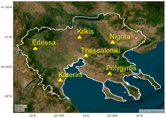
Figure 1.
The newly established GeoNetGNSS CORS network in the region of Central Macedonia.
In the frame of this study, the primary focus was to calculate a high-accuracy, 1 cm level, regional gravimetric geoid model in support of the GeoNetGNSS CORS, based on heterogeneous gravity data for both land and marine areas. The available land gravity database for the region [6] was deemed not suitable to carry out such a high-accuracy geoid determination, given the fact that the data stem from historical databases, have been collected over more than 60 years, and have voids. In this context, considering the area’s geological complexity and existing gaps in the available gravity data that have been used in other geoid calculations [7,8,9,10,11,12], specialized gravity surveys have been planned and conducted in the area under study [6].
This work is split into four sections. The first section describes the dedicated gravity surveys, measurement techniques, and formation of the final gravity database, aiming at enhancing the existing available land gravity observations over the RCM and, especially, around the CORS stations. Then, the second and main section focuses on developing a high-precision, high-resolution geoid model for the broader area of the RCM, followed by its validation with GNSS/leveling data and the estimation of a hybrid, after deterministic and stochastic fit, geoid model, which will be used as reference for related engineering work. Section 2 outlines the area under study, gravity measurements, and relative gravity data processing. Section 3 provides the findings from the local gravity data collection and the development of the final gravity database to be used for geoid modeling. The final section summarizes the geoid calculation both with spectral and stochastic techniques, while it also provides the validation of the final model through a rigorous comparison against a network of GNSS/leveling benchmarks distributed across Northern Greece. Finally, the determination of the hybrid geoid model is outlined and its validation is presented. The entire processing scheme followed for gravity data acquisition and processing, gravimetric geoid determination and validation, and hybrid geoid modeling is outlined in Figure 2.
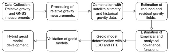
Figure 2.
An outline of the procedure for gravity data collection, processing and geoid determination.
2. Study Area, Data Collection, and Gravity Database
2.1. Study Area
The focus area is the RCM in Northern Greece, which despite being primarily a lowland area, is characterized by diverse topography, ranging from an extensive coastline to mountainous terrains like Mount Olympus to the south (highest top of Greece), Vorras to the north (third-highest top), and Mount Athos in the south-east part, which poses significant challenges for geoid modeling. The geographic boundaries of Central Macedonia extend from a minimum latitude of 39.5° N to a maximum latitude of 41.5° N, and from a minimum longitude of 22.0° E to a maximum longitude of 24.5° E. However, in order to prevent edge effects [12,13,14,15] during geoid modeling in the main focus area, the computation region has been extended from 38.4° N to 42.3° N and from 20.2° E to 25.6° E.
2.2. Relative Gravity Measurements
The development of the regional gravimetric geoid model for Central Macedonia involved the integration of extensive databases, including gravity measurements and GNSS observations, aiming to gather new data close to CORS and fill in places where the current land free-air gravity anomaly database of the Laboratory of Gravity Field Research and Applications (GravLab) has gaps, voids, and data of lower quality [8,10,11,12]. This database mainly consists of historical gravity data for Greece and surrounding countries, shipborne gravity data, and terrestrial gravity data collected by GravLab in the frame of various research projects [16,17,18,19]. The necessary pre-processing steps regarding the gravity data evaluation and validation in terms of their consistency with the used geodetic reference system, tide system, and gravity reference system have been performed so as to form a consistent and homogeneous dataset [10,12]. All the available land and marine gravity data were validated and cleaned by removing blunders and erroneous observations employing a least squares collocation (LSC) [20] approach within a remove–compute–restore (RCR) procedure [21]. This pre-processing analysis resulted in a unified and consistent gravity database with 34,683 point gravity values in GRS80 [22], IGSN71 [23], and the tide free system [24,25] (see black dots in Figure 3).
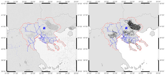
Figure 3.
The study area and gravity data distribution. Left: 36,483 historical (black dots) and 2490 new (blue dots) gravity observations across the broader region. Right: Subset of 5100 historical (black dots) and 1893 new (blue dots) land observations within the area under study (red line).
As it can be seen from Figure 3, the available land gravity database has an overall good distribution in the eastern and central-west part of the area, but significant voids in the Chalkidiki peninsula, the north-west part, and close to Olympus Mountain. Given this, relative gravity surveys have been planned to cover, as homogeneously as possible, the entire study region, with a particular focus on areas with significant topographic gradients and around the established CORS stations. For the data collection, GravLab’s Scrintex CG-5 relative gravity meter (S/N 070540268) has been used, which is one of the most well-established instruments for gravity surveys with a reading resolution of less than 1 μGal, an accuracy of less than 5 μGal, and a residual drift of less than 20 μGal per day [26,27]. As in all relative gravity campaigns intended to determine absolute gravity values at newly established densification points, a reference point with a known absolute gravity value is essential. This ensures that the calculated gravity differences, relative to a known location, can be used to obtain absolute gravity values. In all gravity campaigns, GravLab’s AUT1 absolute gravity station has been used as reference [5,6]. The AUT1 station is situated on the Aristotle University campus premises and was established by GravLab using the Microg-Lacoste A10 (#027) absolute gravity meter, with a recorded gravity value of 980,276,178.42 ± 10.05 μGal. If we assume that the absolute gravity value at AUT1 is determined and denoted with , then, given relative gravity observations between points AUT1 and B, we can estimate the gravity value at the new point B as follows:
Our approach to campaign planning followed a round-trip method, always starting from the AUT1 reference station, occupying a number of densification points, and then completing the campaign at the AUT1 station. This strategy enables the adjustment of residual drift during the day and its distribution across the measured points of that day. Prior to the campaign, the instrument was calibrated for linear drift, X-axis and Y-axis offsets, temperature coefficient, and linear drift. To calculate the daily residual drift, given that m points were measured during the survey, the residual drift was estimated using observations at the initial point AUT1, after corrections for tides, air pressure, height reduction, and temperature, as follows [5]:
where is the residual drift, and and are the gravity observations in mGal at AUT1 at the end of the survey (time ) and the beginning of the survey . We should mention here that the drift after Equation (2) is estimated in , so that after its estimation, the observed gravity difference between station and the initial point is
where and are the observed gravity values at point AUT1, which is the reference station, and Pi, which is the newly established point. They can be corrected for the residual drift as follows:
As a result, the final gravity value after the correction for point i can be estimated as
where is the estimated gravity at point and is the known gravity at the base AUT1. The error at each new point can be calculated through error propagation using the following equation:
where is the accuracy of gravity at point , is the determined accuracy of , and is the propagated error of every gravity observation with the CG-5 (both at the starting point and new points). Considering uncorrelated errors, Equation (6) can be rewritten as
where and are the standard deviations estimated during the relative gravity measurements at the new gravity points.
The relative gravity campaigns have started at the end of August 2022 and finished by the end of May 2023, resulting in a total of 85 days of measurements. The instrument linear drift was estimated every month, 9 times in total, at the premises of the Thessaloniki Seismological Station [28] (TSS). TSS was specifically selected as it offers increased stability and negligible seismic noise due to the bedrock that the station is built on and the existence of a concrete slab that hosts the TSS instruments. The estimation of the drift was obtained by performing cyclic 60 sec measurements, with a relaxation interval between measurements at 5 s, while each measurement session for drift determination lasted 24 h. After this, the estimated stationary drift value was used to adjust the drift correction factor, previously determined on the instrument according to the CG-5 user manual [29]. For each campaign, the next criteria were followed:
- o
- The CG-5 was leveled with an accuracy of >10 arcseconds.
- o
- The CG-5 height was measured with an accuracy of 1 mm on all three sides.
- o
- Each new point was marked.
- o
- At each occupation, the CG-5 was left undisturbed for 10 min to allow the measuring system to settle and reach the ambient temperature.
- o
- At each point, 6 measurement cycles were performed to have at least 5 valid measurement cycles at the time of the measurements.
- o
- During measurement at each point, the following criteria were satisfied:
- The ambient temperature, air pressure, and height of the gravimeter have been measured.
- The leveling of the gravimeter was continuously monitored to not exceed 10 s.
- At points where the difference in readings due to disturbances was greater than 15 μGal, the measurements were repeated.
- The CG-5 was protected with an umbrella from sun and wind during the measurement process.
In total, 2490 new gravity data were established and measured with their 3D location being determined with network real-time kinematic (NRTK) GNSS measurements. At every point, 10 epochs of 1 s GNSS observations have been collected using the virtual reference station (VRS) employing the Hellenic Positioning System service (HEPOS) [30]. Error propagation has been carried out with Equation (9) for all 2490 newly acquired gravity benchmarks, where, given the accuracy of the absolute gravity value at AUT1 (), a mean accuracy at the 26.21 μGal level and a standard deviation at the 4.36 μGal have been achieved.
After determining the gravity value at each location, gravity anomalies and free-air gravity anomalies have been calculated. The gravity anomaly at each point was determined as follows:
where stands for the normal gravity in the GRS80 ellipsoid evaluated with Somigliana’s formula [31], while free-air gravity anomalies were estimated through the mean normal gradient of :
In Equation (9), is the orthometric height of the point location referring to the TG station at Piraeus harbor where the zero level for Hellenic vertical datum is located [32,33,34].
After finishing the data processing, the final gravity values and their accuracy at the new points were estimated. The final gravity database (see Figure 3) utilized consisted of 38,973 point free-air gravity anomalies, comprising 36,483 historical (black dots) measurements and 2490 newly (blue dots) collected observations with their statistics reported in Table 1. Within the specific study area of the RCM (see Figure 3, right panel), 6993 land gravity observations were employed, which included 5100 historical (black dots) measurements and 1893 newly (blue dots) collected data.

Table 1.
Statistics of the free-air gravity anomalies (original and new data) for the area. Unit: mGal.
For the validation of the final geoid model developed, 462 GNSS/leveling BMs located within or up to 50 km outside the main focus area of the RCM were used (see Figure 4). The ellipsoidal heights of these BMs have been determined as part of the Hellenic Cadastre project by Ktimatologio S.A., which conducted a nationwide GNSS survey to gather static GNSS data on geodetic BMs, achieving a mean accuracy of 2–5 cm [33]. The orthometric heights, at the BMs provided by the HMGS, are formally reported to have an accuracy of 1–2 cm; however, their actual accuracy remains largely uncertain [33,34]. Table 2 tabulates the statistics of the 462 GNSS/leveling BMs, while it should be mentioned that the geoid heights mentioned in this table are formed as ; hence, these represent a geometric computation of geoid heights and not gravimetric ones.
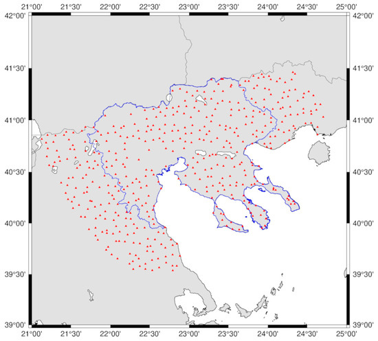
Figure 4.
Location of GNSS/leveling data (red triangles) for geoid validation inside or up to 50 km away from the RCM (blue line).
Table 2.
Statistics of GNSS/leveling data inside or up to 50 km away from the RCM used geoid validation. Unit: [m].
3. Methodology and Geoid Development
The gravimetric geoid was based on the previously described new and historical gravity data, GNSS/leveling observations, satellite altimetry data from DTU 2021 [35] for marine areas, and databases on the topography and bathymetry of the region [9,10]. Two main approaches have been followed to estimate the gravimetric geoid in the area, employing both spectral, through the fast Fourier transform (FFT) evaluation of Stokes’ integral [20], as well as stochastic methods with LSC [21]. Both approaches have been extensively used in geoid related studies during the last 30 years [5,15,20,21,36,37] and rely on the use of residual gravity anomaly values as input data. Residual gravity anomalies are constructed employing the RCR concept [5,21], after the removal of the contribution of a GGM and of the topographic effects. In the removal step of RCR, the long wavelengths of the gravity field spectrum are described by a GGM in the form of a spherical harmonic expansion to some degree and order. The GGM contribution has been assessed from XGM2019e, which incorporates data from GOCO06s in the longer to medium wavelengths of the spectrum and gravity data for the shorter wavelengths [38]. XGM2019e was employed to its full harmonic degree of expansion ( as it provided the most accurate results over the Greek area in recent similar studies [5,8]. Reduced gravity anomalies have been estimated as follows:
where
is the contribution of the GGM. In Equation (11), a is the semi-major axis of the ellipsoid, M is Earth’s mass, G is the gravitation constant, (cosθ) are the Legendre functions, and are the fully normalized spherical harmonic coefficients of the disturbing potential. By replacing , Equation (10) can be written as follows:
The purpose of the removal process is to create a field with residual gravity anomalies (Δgres) that is sufficiently smooth for prediction after removing the higher frequencies that correspond to the area’s topography and bathymetry. The residual gravity anomalies are treated as a stationary random signal; hence, the errors of the input signal are random with a zero or close to zero mean. Among the various topographic reductions methods, the residual terrain model (RTM) reduction has been employed, as it generates smooth gravity anomaly residuals [39,40]. A major benefit of this method is that the magnitude of the value to be restored in the final step, when calculating geoid heights, is significantly smaller than the indirect effect on the geoid seen with other methods, and it does not require any assumptions about isostatic compensation. For the RTM reduction, the spectral approach was followed [41], combining a spherical harmonics expansion of the Earth’s topographic potential and ultra-high resolution RTM effects from a pre-computed global model [42]. As XGM2019e, in our approach, was evaluated up to its maximum degree, only the ultra-high resolution RTM effects from the ERTM2160 [42] have been calculated as follows:
and as a result, the final estimated residual gravity field was derived as
which can be written as
Based on the estimated residuals from Equation (15), various geoid models have been evaluated with LSC and FFT, while the two different methods have been employed in order to ensure redundancy and allow for cross-checking between them. In the computation process, residual geoid heights (Nres) are estimated from the residual gravity anomalies Δgres and are then used to calculate the final geoid during the restore process. The restore process involves adding back the previously removed signals to the residual geoid heights. The determined geoid model, whether computed through LSC or FFT, was generated on a 1 arcmin × 1 arcmin grid over a broader region surrounding RCM. The prediction using LSC was performed as follows [43]:
where are the (observations) and is their covariance matrix, is the cross-covariance matrix derived from the observed with the predicted , and is the noise of . LSC allows the simultaneous determination of the error covariance matrix as follows [21,43]:
where is estimated from the predicted . To calculate the needed matrices in Equations (16) and (17), an analytical covariance function, which will describe the statistical characteristics of the gravity field in the region under study, should be estimated. Within our work, we use the analytical model of Tscherning and Rapp [43], which, from the covariance function of the disturbing potential T and by covariance propagation, allows the computation of all needed auto- and cross-covariance functions as follows:
In Equation (18), are degree variances up to the full power of the reference GGM, is the so-called radius of the Bjerhammar sphere, denote the Legendre polynomials, and are the degree variances adopted above the maximum degree of the GGM expansion until infinity. Then, for the determination of the final geoid heights from LSC, the contribution of XGM (NXGM) and the one of topography (NTOPO) through RTM reduction are restored to derive the final geoid heights through the following equation:
In the case of the spectral evaluation with FFT [20,44], the Wong–Gore modification of the Stokes kernel is applied [45], after applying 100% zero padding in all directions. In this case, the residual geoid heights are derived from the as follows:
where is the band-limited Stokes kernel to the maximum degree of the GGM expansion, and and denote the number of parallels and meridians (rows and columns of the available gravity residual grid) with spacing and :
In Equation (21), is the classical Stokes kernel, L is the degree of expansion below which terms are to be removed, is the Legendre polynomial, and is the spherical distance between the points i, j. Then, the final geoid heights from FFT are given as
Reduced and Residual Gravity Fields
Through Equation (12) the reduced free-air gravity anomalies to XGM2019e d/o 2190 have been computed, with Table 3 tabulating the statistics of the original gravity, topography, and XGM2019e contribution along with the reduced and residual gravity anomalies. As it can be seen, XGM2019e reduced the mean value from 14.83 mGal to −2.704 mGal, while a further reduction is noticed in the std, which dropped from 44.135 mGal in the original field to 14.426 mGal for the reduced one. This is also obvious in Figure 5, where the original, the reduced, and the residual gravity anomaly fields are depicted. The low and medium frequencies of XGM2019e successfully captured most of the regional and local gravity field characteristics in the area, although some higher frequencies still remain, especially over the mountainous areas of Olympus, Pindos, and Korab in Albania. For the calculation of the residual gravity field, the RTM effects were removed from the reduced gravity using (Equation (14)). The ultra-high topographic effects of have a mean value of −5.479 mGal and a std of ±16.483 mGal and manage to smooth further the reduced field and improve the statistics, resulting in a mean value close to zero (−0.396 mGal) and a std of ±10.179 mGal. The mean value being at the sub-mGal level indicates that the residual field can indeed be regarded as unbiased while the std of the entire field (including both land and marine data, and gravity data from neighboring countries) is close to the one (±4.18 mGal) estimated by [11], where local free-air gravity anomalies were combined with GOCE SGG data.
Table 3.
Statistics of the original gravity anomalies, XGM2019e, and topographic contributions. Reduced and residual gravity anomalies. Unit: mGal.
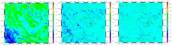
Figure 5.
The original (left), reduced (middle), and residual gravity anomalies (right). Unit: mGal.
For both the reduced and residual gravity fields, the empirical covariance functions have been estimated and are depicted along with the analytical covariance function for the residual gravity anomalies in Figure 6. The variance from 425.74 mGal2 in the reduced field drops to 186.29 mGal in the residuals, while the correlation length is 7.88 km for the reduced and 17.09 km for the residual gravity anomalies. Both statistical measures indicate that, indeed, the residual field is smooth and can be used for prediction with LSC and FFT. Finally, for the LSC modelling process, the analytical covariance function model presented in Equation (18) was fitted to the empirical model with the analytical model having a variance of 186.29 mGal and a correlation length of 12.52 km.
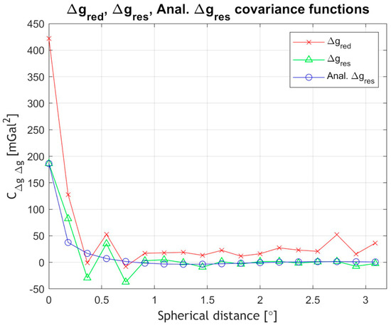
Figure 6.
Empirical covariance function for reduced gravity anomalies and residual gravity anomalies. Analytical covariance function for residual gravity anomalies. Unit [mGal2].
4. Geoid Models Determination and Validation
As already mentioned, two different approaches have been followed for geoid determination, with the first test employing the FFT evaluation of the Stokes kernel with a Wong–Gore modification. As all spectral methods require gridded data, a 1′ x 1′ grid from the available point residual gravity anomalies has been determined using kriging, given its similarities to LSC, incorporating the individual variances and correlation length of the empirical covariance function mentioned in the previous section. As previously stated, for the validation of the geoid model developed, 462 GNSS/leveling BMs, located within or up to 50 km outside the RCM, were used. In order to select the optimal cut-off degrees for the Wong–Gore kernel and investigate the number of parallels used in the 2D-FFT as well as whether the removal of the residual gravity data mean value is significant, various tests have been performed. We investigated the use of 1, 3, and 9 parallels in the 2D-FFT evaluation of the Stokes kernel, the removal or not of the mean value, and the cut-off degree of the Wong–Gore kernel starting from degree/order (d/o) 60 up to d/o 180 [46,47]. Other cut-off degrees have been examined as well, but only the results for the aforementioned investigations are reported as being the optimal ones. All these options have been evaluated having as a metric of their external accuracy the differences to the GNSS/leveling geometric geoid heights. Table 4 reports the statistics of the geoid height differences between the various 2D-FFT Wong–Gore gravimetric geoid models and the GNSS/leveling data. For ease of reference, the first column in Table 4 represents the name of each model developed. The two first values correspond to the harmonic degrees for the tapering, the third value corresponds to the number of parallels used with t signifying the mean value removal, and f stands for no mean value removal. From the statistics in Table 4, it is apparent that the removal, or not, of the mean of the residual gravity plays little role in the mean differences to the GNSS/leveling data, as the differences between the various options are at the few-mm level. Moreover, the tapering between degrees 60 and 140 is comparable and the differences are very small, giving mm-level improvements in the std, so that the overall best solution selected was with the tapering to the band between d/o 100 and 120. In terms of the use of more than one parallel in the FFT evaluation, it is clear that the influence is small, being, again, at the few mm level. Hence, the solution with the tapering to d/o 100–120 has been used, without removal of the mean value of the gravity residuals and with the use of one parallel, which corresponds to a rigorous 1D-FFT evaluation of the Stokes kernel on the sphere along each parallel [46,47].
Table 4.
Statistics of the geoid height differences between the various 2D-FFT Wong–Gore gravimetric geoid models and the GNSS/leveling data. Gray denotes the selected truncation. Units: [m].
The second approach for geoid determination is based on LSC and the use of the original residual gravity anomalies with the analytical covariance function depicted in Figure 6. Table 5 tabulates the differences to the GNSS/leveling BMs for the two regional geoid models, i.e., the FFT- and LSC-based ones, while the LSC geoid estimation errors are also reported. For the LSC geoid, a std of 13.1 cm is achieved, which is 1.2 cm higher than that of the FFT solution, while the mean of the differences is at the 20.3 cm level compared to the 12.2 cm level for the FFT geoid. These slightly worse statistics for the LSC approach are probably due to the inhomogeneous distribution of the gravity data, especially over rougher terrain (western part of the area), but the difference can be regarded as negligible. To quantify the improvement brought by the acquisition of new gravity data in the geoid model development, Table 5 reports, as well, the statistics of the differences to the GNSS/leveling data of the GreekGeoid2010 [12]. This nationwide geoid was computed with the same methodology, i.e., employing the RCR approach, an FFT evaluation of Stokes’ kernel function, and an RTM-based evaluation of the topographic effects. Hence, the reduced std for the newly determined geoid compared to GreekGeoid2010, from 15.0 cm to 11.9 cm signals the improvement brought by the new gravity data. Even the new LSC geoid, which, given the sparse distribution of the data, cannot achieve the same level of accuracy as the FFT geoid on the final 1′ x 1′ (~1.8 km) grid, is two times better compared to the latest gravimetric geoid for the country. This clearly shows that the acquisition of new high-quality local gravity data can contribute to geoid improvement significantly. One point that is worth mentioning is that the remaining bias of 12.2 cm represents the bias of the Hellenic vertical datum, as realized by this regional set of GNSS/leveling data, relative to the conventional [4] that has been used as reference in this study. The differences are formed as ; hence, the positive difference implies that the Greek vertical datum in North Greece is below the IAG conventional global geoid. Of course, given the peculiarities of the Greek vertical datum and the existing offsets and tilts [5,8,31,33,34,48], this bias is valid only for the area investigated, as it cannot represent the entire Greek territory.
Table 5.
Statistics of the geoid height differences between old geoid model (GreekGeoid2010), optimal 1D-FFT Wong–Gore gravimetric geoid model, LSC geoid model, and GNSS/leveling data. Units: m.
Figure 7 depicts the differences of the new geoid models developed along with the old geoid model and the GNSS/leveling data. As it can be noticed, the new geoid models show better agreement, compared to the old geoid model, and show better results against GNSS/leveling for the entire area of the RCM. The FFT-based model provides a geoid height difference to the GNSS/leveling data at −10 cm and +20 cm in the most part of the region, while larger values are found in the borders of the area. On the other hand, the LSC geoid has differences to the GNSS/leveling data, especially in the central part of RCM, which reach up to ~20–30 cm, while its worst performance is found, again, close to the borders with the other Balkan countries. This is probably due to the few land gravity data available over the northern part of the area and the inferior performance of the GGM-derived gravity anomalies used as fill-in for the other countries.
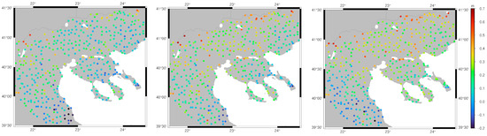
Figure 7.
Differences of the gravimetric FFT geoid model (left), gravimetric LSC (center), and GreekGeoid2010 (right) to the GNSS/leveling data. Unit [m].
Hybrid Geoid Model Development
As already mentioned, the scope of the present study is not to just reach the overall best gravimetric geoid, but to determine a geoid model that will be useful for GNSS-based orthometric height development. This leads to the determination and modeling of a so-called hybrid geoid model, i.e., a geoid model that is fitted to some known geometric geoid heights, in our case, the available GNSS/leveling data. This will not be a physically meaningful geoid, i.e., representing a strict geopotential surface, but a geoid model that will absorb any differences to the GNSS/leveling data and will manage to provide accurate orthometric heights using GNSS. For that, a two-step approach was followed, during which, first, a deterministic fit to the GNSS/leveling data has been performed, using various parametric models, in order to model any systematic differences between the FFT-based geoid and the GNSS/leveling data, and then, an LSC-based modeling of the residual stochastic signal was performed [49,50]. It should be noted that contrary to the usual fit of geoid models to GNSS/leveling data, where we aim at a parametric model with parameters that have a physical meaning [5,51], our goal was to compute a hybrid geoid model that would have the smallest residual errors to the available GNSS/leveling data. This is important so that the professionals using the hybrid geoid model, onboard their GNSS receivers, will realize the existing national vertical datum in the area, despite its biases and tilts.
In that sense, an observation equation can be formed between the GNSS/leveling and gravimetric geoid heights to evaluate their absolute and relative differences for all formed baselines as
with the main results to be evaluated being the mean and the std of the differences. The former shows, as mentioned, the gravimetric geoid bias relative to the Greek vertical datum as realized in Northern Greece, and the latter represents an external accuracy estimate. Similarly, the relative differences are evaluated, either in an absolute Equation (24) or a relative Equation (25) sense, as follows:
Equation (23) in matrix notation can be written as:
where A is the design matrix, x is the matrix of the unknowns, s denotes stochastic signal, and v denotes the errors of the observations b. The selection of the parametric model to be used in this least-squares adjustment scheme varies from simple north-south tilt models to four- and five-parameter similarity transformation and polynomials ones [31,50,52]. Then, the unknown deterministic parameters of the transformation model can be determined as follows:
Then, the adjusted residuals after the deterministic fit,
which represent the remaining unmodeled residual differences between the GNSS/leveling and gravimetric geoid heights, can be treated stochastically with LSC in order to determine the final hybrid geoid heights as a combination of stochastic and deterministic modeling:
With the present study, the deterministic part has been modeled with polynomial models of the form
Which, for a second-order polynomial is
And, for a third-order model, becomes
More simple choices for the parametric treatment of the residuals, with physical meaning of the derived adjusted parameters, were also checked, such as the north-south tilt model:
Finally, among other choices, the ones resembling the extended seven-parameter Helmert similarity transformation model with four and five parameters have been tested, although the computed parameters have no physical meaning in case of 1D networks. The four- and five-parameter similarity transformation models are given through Equations (34) and (35) [31]:
After the deterministic and stochastic treatment of the residuals and the adjustment of the gravimetric geoid to the existing GNSS/leveling data, the hybrid geoid is a geoid solution that optimally aligns with the latter and yields minimal residuals. Table 6 tabulates the statistics of the geoid height differences between the FFT gravimetric geoid model and the GNSS/leveling data before and after the fit. Based on the fit to the parametric models and without performing a 2σ test nor a 3σ in order to remove any possible blunders from the available BMs, the N-S tilt reduces the std of the differences to 11.4 cm of the four- and five-parameter models to 10.6 cm, while the second-order polynomial decreases it to 10.1 cm and the third-order decreases it further, down to 10 cm. As the improvement offered by the third-order polynomial is 1 mm only, the final choice for the deterministic treatment of the residuals was the second-order polynomial model, with the residual signal presented in Table 6 being the one to be used as input for the stochastic modeling. As a further validation, the absolute and relative differences of the adjusted residuals after the deterministic fit have been also computed. For the absolute differences of the residuals after the second-order polynomial fit, 83.1% of the differences are lower than the 2 level and 54.8% are lower than the 1 level (see Figure 8). In terms of the relative difference, a 11.3 ppm relative accuracy is found for baselines between 0 and 10 km, which then reduced to 6.8 ppm for baselines between 10 and 20 km; then, it is below 4 ppm (see Figure 8).
Table 6.
Statistics of the geoid height differences between the 1D-FFT gravimetric geoid model and the GNSS/leveling data after deterministic fit. Units: [m].
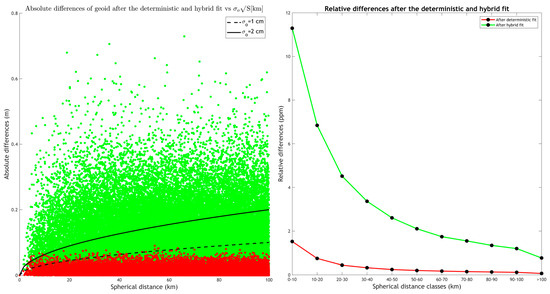
Figure 8.
Absolute (left) and relative differences (right) of the hybrid geoid model after the deterministic fit (green) and after the deterministic and stochastic fit (red).
For the calculation of the final hybrid geoid model, after the deterministic fit with the second-order pol., a collocation approach employing exponential (Models A–D, as in Equations (36)–(39)), second-order Gauss–Markov (Model E, as in Equation (40)), and third-order Gauss–Markov (Model F as in Equation (41)) covariance functions was used [50] to model the stochastic residuals. Figure 9 depicts the empirical and analytical covariance function models of the deterministically fitted residuals. It should be noted that given the small magnitude of the residuals, a zoomed version is plotted only up to a spherical distance of 50 km as, after that, all covariance functions tend to zero. In the models below, ψ denotes the spherical distance, r the planar distance, d the characteristic distance ( being the correlation length), and the variance. The rest are parameters to be determined, so that the analytical model will fit the empirical one.
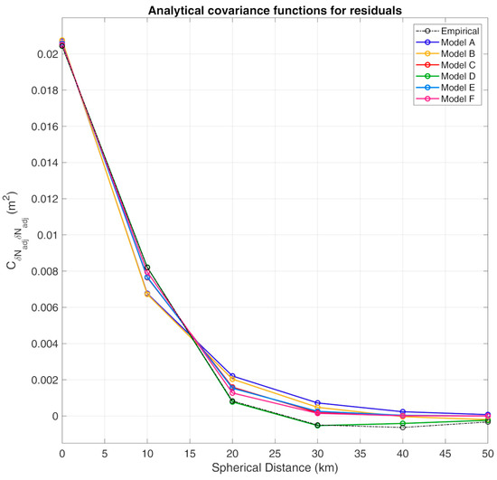
Figure 9.
Empirical and analytical covariance functions, after the deterministic fit, of the adjusted residuals between the FFT gravimetric geoid and GNSS/leveling geoid heights. Unit [m2].
Therefore, six deterministically and stochastically treated, hybrid geoid models (Models A–F) have been determined, with the statistics of their differences to the GNSS/leveling geoid heights being tabulated in Table 7. Model F (third-order Gauss–Markov) provides the best results, as its fits to the GNSS/leveling data with a std of just 1.1 cm, while the maximum difference is at the 5.5 cm and the minimum difference is at the −3.6 cm level. For the further evaluation, absolute and relative differences were also estimated, after the parametric and stochastic modeling, with 99.8% and 99.9% of the differences being lower than level, respectively. In terms of the relative differences, baselines between 0 and 10 km have a difference of 1.5 ppm, which, for baselines as short as 5 km, are better than 2 ppm (see Figure 9). The relative differences drop below the 1 ppm level (1 cm per km leveling traverse) for baselines larger than 14 km. The final hybrid geoid model for the area under study, being the one after the deterministic fit with the second-order polynomial and the stochastic treatment of the residuals with the third-order Gauss–Markov model, is presented in Figure 10.
Table 7.
Statistics of the geoid height differences between the 1D-FFT gravimetric geoid model and the GNSS/leveling data after the deterministic and stochastic fit. Units: [m].
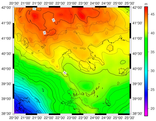
Figure 10.
The final hybrid geoid model.
5. Conclusions
The main focus of this study was the calculation of a regional high-accuracy and high-resolution gravimetric geoid model for the region of Central Macedonia in Northern Greece, to support orthometric height determination with GNSS in the frame of the establishment of a new network CORS. Several models have been estimated, based on both historical and recently collected gravity observations collected through dedicated gravity surveys. The development of the geoid was based on the classical RCR technique, while both spectral (FFT) and stochastic (LSC) methods have been used. The low and high frequencies of the gravity field spectrum were treated using XGM2019e as a GGM and topographic effects following the classical and spectral RTM approaches. This was followed by the prediction of residual geoid heights and the restoration of the effects previously removed to derive the final gravimetric geoid model. Various geoid models have been estimated and validated against available collocated GNSS/leveling observations to determine, on one hand, the optimal cut-off degree for the spectral evaluation of Stokes’ integral, and on the other, to have a quantitative validation in terms of the absolute and relative differences achieved.
The newly determined gravimetric geoid presented an improvement by ~4 cm in terms of the std of the differences to the GNSS/leveling data, compared to the previous nationwide geoid model, before any deterministic and stochastic fit. This improvement marks the contribution of the new high-accuracy gravity data over the study area, and the expected contributions of gravity surveys to geoid modeling, especially over areas where the current gravity data holdings show voids. This is of particular interest to regional gravity and geoid approximation as well as to the realization of the International Height Reference System (IHRS), when new high-accuracy gravity data are to be collected. As the goal was to estimate a geoid for use with GNSS applications, the residuals of the gravimetric geoid relative to available GNSS/leveling data have been treated with a hybrid deterministic and stochastic approach. The deterministic fit was used to model any systematic differences between the gravimetric and geometric geoid heights, which, without performing any 2σ test and 3σ in for blunder removal, has given a std of 10.1 cm after a second-order polynomial fit. A total 83.1% of the differences were lower than the 2 and 54.8% were lower than the 1 error, while a 11.3 ppm relative difference was achieved for baselines between 0 and 10 km. The latter is close to the 1 cm per km relative error, which signals that even after a deterministic fit, the gravimetric geoid determined is of high accuracy.
After the deterministic fit, a stochastic modeling of the adjusted residuals was performed while the final hybrid geoid model was computed based on the hybrid deterministic and stochastic treatment of the residuals. Various choices for the selection of the analytical covariance function to be used have been investigated, with a third-order Gauss–Markov model giving the optimal fit. From the results acquired, the final absolute hybrid geoid model accuracy reaches the ~1 cm level, while 99.8% and 99.9% of the height differences are below the 1 and 2 standard errors, respectively, for the absolute differences along the formed baselines. These mark a significant contribution to GNSS/leveling, as the 1 cm per square root km level is also within the accuracy of most common leveling surveys and the target for the realization of the IHRS. For baselines between 0 and 10 km, the relative differences were at the 1.5 ppm level, which was reduced to being below the 1 ppm level for baselines larger than 14 km. These translate to a ~1 mm/km relative height error, which suffices for surveying and engineering applications.
Author Contributions
Conceptual design of the experiment and analysis, G.S.V., I.N.T. and D.A.N.; gravity campaign data acquisition, D.A.N., E.G.M., G.S.V., I.N.T. and E.A.T.; gravity reductions and geoid estimation by FFT and LSC, D.A.N. and G.S.V.; geoid validation, D.A.N. and I.N.T.; writing—original draft preparation, D.A.N. and G.S.V.; writing—review and editing, E.A.T., A.I.T., E.G.M., D.R. and V.P.; visualization, D.A.N.; supervision, G.S.V.; project administration, I.N.T., G.S.V., D.R. and V.P.; funding acquisition, I.N.T., G.S.V., D.R. and V.P. All authors have read and agreed to the published version of the manuscript.
Funding
This research was funded as part of the project «GeoNetGNSS» (Project code: ΚΜΡ6-0071139) implemented under the framework of the Action «Investment Plans of Innovation» of the Operational Program «Central Macedonia 2014 2020», which is co-funded by the European Regional Development Fund and Greece.
Data Availability Statement
The GNSS/leveling data have been provided by the Hellenic Cadastre S.A. in the frame of a memorandum of understanding with the Department of Geodesy and Surveying, AUTH. XGM2019e has been downloaded from the ICDEM service (http://icgem.gfz-potsdam.de/, accessed on 9 May 2023). Historical gravity data over the area are available by GravLab Database. The data collected during the gravity surveys over Region of Central Macedonia are available on request from the authors.
Conflicts of Interest
The authors declare that the research was conducted in the absence of any commercial or financial relationships that could be construed as potential conflicts of interest.
References
- Matsuo, K.; Kuroishi, Y. Refinement of a gravimetric geoid model for Japan using GOCE and an updated regional gravity field model. Earth Planets Space 2020, 72, 33. [Google Scholar] [CrossRef]
- Featherstone, W.E. Absolute and relative testing of gravimetric geoid models using Global Positioning System and orthometric height data. Comput. Geosci. 2001, 27, 807–814. [Google Scholar] [CrossRef]
- Sjöberg, L.E.; Abrehdary, M. Geoid or Quasi-Geoid? A Short Comparison. In X Hotine-Marussi Symposium on Mathematical Geodesy HMS 2022; Freymueller, J.T., Sánchez, L., Eds.; International Association of Geodesy Symposia; Springer: Berlin/Heidelberg, Germany, 2023; Volume 155. [Google Scholar] [CrossRef]
- Sánchez, L.; Barzaghi, R.; Vergos, G. Operational Infrastructure to Ensure the Long-Term Sustainability of the International Height Reference System and Frame (IHRS/IHRF); International Association of Geodesy Symposia; Springer: Berlin/Heidelberg, Germany; New York, NY, USA, 2024. [Google Scholar] [CrossRef]
- Vergos, G.S.; Tziavos, I.N.; Mertikas, S.; Piretzidis, D.; Frantzis, X.; Donlon, C. Local Gravity and Geoid Improvements around the Gavdos Satellite Altimetry Cal/Val Site. Remote Sens. 2024, 16, 3243. [Google Scholar] [CrossRef]
- Natsiopoulos, D.A.; Mamagiannou, E.G.; Triantafyllou, A.; Tzanou, E.A.; Vergos, G.S.; Tziavos, I.N.; Ramnalis, D.; Polychronos, V. Newly Acquired Gravity Data in Support of the GeoNetGNSS CORS Network in Northern Greece. In Gravity, Positioning and Reference Frames. REFAG 2022; Freymueller, J.T., Sánchez, L., Eds.; International Association of Geodesy Symposia; Springer: Berlin/Heidelberg, Germany, 2023; Volume 156. [Google Scholar] [CrossRef]
- Wang, Y.M.; Sánchez, L.; Ågren, J.; Huang, J.; Forsberg, R.; Abd-Elmotaal, H.A.; Ahlgren, K.; Barzaghi, R.; Bašić, T.; Carrion, D.; et al. Colorado geoid computation experiment: Overview and summary. J. Geod. 2021, 95, 127. [Google Scholar] [CrossRef]
- Grigoriadis, V.N.; Andritsanos, V.D.; Natsiopoulos, D.A.; Vergos, G.S.; Tziavos, I.N. Geoid Studies in Two Test Areas in Greece Using Different Geopotential Models towards the Estimation of a Reference Geopotential Value. Remote Sens. 2023, 15, 4282. [Google Scholar] [CrossRef]
- Grigoriadis, V.N.; Andritsanos, V.D.; Natsiopoulos, D.A. Validation of Recent DSM/DEM/DBMs in Test Areas in Greece Using Spirit Leveling, GNSS, Gravity and Echo Sounding Measurements. ISPRS Int. J. Geo-Inf. 2023, 12, 99. [Google Scholar] [CrossRef]
- Grigoriadis, V. Geodetic and Geophysical Approximation of the Earth’s Gravity Field and Applications in the Hellenic Area. Ph.D. Thesis, Aristotle University of Thessaloniki, Thessaloniki, Greece, 2009. (In Greek). [Google Scholar]
- Natsiopoulos, D.A.; Mamagiannou, E.G.; Pitenis, E.A.; Vergos, G.S.; Tziavos, I.N. GOCE Downward Continuation to the Earth’s Surface and Improvements to Local Geoid Modeling by FFT and LSC. Remote Sens. 2023, 15, 991. [Google Scholar] [CrossRef]
- Tziavos, I.N.; Vergos, G.S.; Grigoriadis, V.N. Investigation of topographic reductions and aliasing effects on gravity and the geoid over Greece based on various digital terrain models. Surv. Geophys. 2010, 31, 23–67. [Google Scholar] [CrossRef]
- Novák, P. Geoid determination using one-step integration. J. Geod. 2003, 77, 193–206. [Google Scholar] [CrossRef]
- Jekeli, C.; Serpas, J.G. Review and numerical assessment of the direct topographical reduction in geoid determination. J. Geod. 2003, 77, 226–239. [Google Scholar] [CrossRef]
- Tziavos, I.N. Comparisons of spectral techniques for geoid computations over large regions. J. Geod. 1996, 70, 357–373. [Google Scholar] [CrossRef]
- GOCESeaComb Project. Available online: http://olimpia.topo.auth.gr/GOCESeaComb/ (accessed on 24 October 2024).
- GOCE for HSU and DOT. Available online: http://olimpia.topo.auth.gr/GOCE_HSU_DOT_G/ (accessed on 24 October 2024).
- GeoGravGOCE Project. Available online: http://olimpia.topo.auth.gr/GeoGravGOCE/index.html/ (accessed on 24 October 2024).
- ModernGravNet Project. Available online: http://olimpia.topo.auth.gr/moderngravnet/ (accessed on 24 October 2024).
- Sansò, F.; Sideris, M.G. The Local Modelling of the Gravity Field by Collocation. In Geoid Determination: Theory and Methods; Lecture Notes in Earth System Sciences; Springer: Berlin/Heidelberg, Germany, 2013; Volume 110, pp. 203–258. [Google Scholar] [CrossRef]
- Sansò, F. Observables of physical geodesy and their analytical representation. In Geoid Determination: Theory and Methods; Sansò, F., Sideris, M.G., Eds.; Lecture Notes in Earth System Sciences; Springer: Berlin/Heidelberg, Germany, 2013; Volume 110. [Google Scholar]
- Moritz, H. Geodetic Reference System 1980. J. Geod. 2000, 74, 128–133. [Google Scholar] [CrossRef]
- Morelli, C.; Gantar, C.; Honkasalo, T.; McConnell, R.K.; Tanner, I.G.; Szabo, B.; Uotila, U.; Whalen, C.T. The International Gravity Standardisation Net 1971 (IGSN71); Special Publication 4; IAG: Paris, France, 1974. [Google Scholar]
- Ekman, M. Impacts of geodynamic phenomena on systems for height and gravity. Bull. Geod. 1989, 63, 281–296. [Google Scholar] [CrossRef]
- Ekman, M. The permanent problem of the permanent tide. What to do with it in geodetic reference systems? Bull. Inf. Marées Terr. 1996, 125, 9508–9513. [Google Scholar]
- Lederer, M. Accuracy of the relative gravity measurement. Acta Geodyn. Geomater. 2009, 6, 383–390. [Google Scholar]
- Yushkin, V.D. Operating experience with CG5 gravimeters. Meas. Tech. 2011, 54, 486–489. [Google Scholar] [CrossRef]
- Vamvakaris, D.A.; Scordilis, E.M. The Seismological Network of Aristotle University of Thessaloniki, Greece (AUTHnet). Summ. Bul. Int. Seis. Cent. 2020, 54, 31–49. [Google Scholar] [CrossRef]
- Scintrex CG-5 Manual. Available online: https://scintrexltd.com/wp-content/uploads/2017/02/CG-5-Manual-Ver_8.pdf (accessed on 1 May 2022).
- Gianniou, M. HEPOS: Designing and Implementing an RTK-Network. Geoinformatics Mag. Surv. Mapp. GYS Prof. 2008, 11, 10–13. [Google Scholar]
- Heiskanen, W.A.; Moritz, H. Physical Geodesy; WH Freeman: San Francisco, CA, USA, 1967. [Google Scholar]
- Grigoriadis, V.N.; Lambrou, E.; Vergos, G.S.; Tziavos, I.N. Assessment of the Greek Vertical Datum: A Case Study in Central Greece. In International Symposium on Gravity, Geoid and Height Systems 2016; Vergos, G., Pail, R., Barzaghi, R., Eds.; International Association of Geodesy Symposia; Springer: Cham, Switzerland, 2017; Volume 148. [Google Scholar] [CrossRef]
- Kotsakis, C.; Katsambalos, K.; Ampatzidis, D. Estimation of the zero-height geopotential level in a local vertical datum from inversion of co-located GPS, leveling and geoid heights: A case study in the Hellenic islands. J. Geod. 2012, 86, 423–439. [Google Scholar] [CrossRef]
- Vergos, G.S.; Erol, B.; Natsiopoulos, D.A.; Grigoriadis, V.N.; Işık, M.S.; Tziavos, I.N. Preliminary Results of GOCE-Based Height System Unification between Greece and Turkey over Marine and Land Areas. Acta. Geod. Geophys. 2018, 53, 61–79. [Google Scholar] [CrossRef]
- Andersen, O.B.; Knudsen, P. The DTU17 Global Marine Gravity Field: First Validation Results. In Fiducial Reference Measurements for Altimetry; Mertikas, S., Pail, R., Eds.; International Association of Geodesy Symposia; Springer: Cham, Switzerland, 2019; Volume 150. [Google Scholar] [CrossRef]
- Schwarz, K.P.; Li, Y.C. What can airborne gravimetry contribute to geoid determination? J. Geophys. Res. 1996, 101, 17873–17881. [Google Scholar] [CrossRef]
- Tscherning, C.C. Geoid Determination by 3D Least-Squares Collocation; Lecture Notes in Earth System Sciences; Springer: Berlin/Heidelberg, Germany, 2013; Volume 110, pp. 311–336. [Google Scholar]
- Zingerle, P.; Pail, R.; Gruber, T.; Oikonomidou, X. The combined global gravity field model XGM2019e. J. Geod. 2000, 94, 66. [Google Scholar] [CrossRef]
- Forsberg, R. A Study of Terrain Corrections, Density Anomalies and Geophysical Inversion Methods in Gravity Field Modelling; Rep. No. 355; Ohio State University: Columbus, OH, USA, 1984. [Google Scholar]
- Tziavos, I.N.; Sideris, M.G. Topographic Reductions in Gravity and Geoid Modeling. In Geoid Determination; Sansò, F., Sideris, M., Eds.; Lecture Notes in Earth System Sciences; Springer: Berlin/Heidelberg, Germany, 2013; Volume 110. [Google Scholar] [CrossRef]
- Hirt, C.; Kuhn, M.; Claessens, S.; Pail, R.; Seitz, K.; Gruber, T. Study of the earth′s short-scale gravity field using the ERTM2160 gravity model. Comput. Geosci. 2014, 73, 71–80. [Google Scholar] [CrossRef]
- Rexer, M.; Hirt, C.; Bucha, B.; Holmes, S. Solution to the spectral filter problem of residual terrain modelling (RTM). J. Geod. 2018, 92, 675–690. [Google Scholar] [CrossRef]
- Tscherning, C.C.; Rapp, R.H. Closed Covariance Expressions for Gravity Anomalies, Geoid Undulations, and Deflections of the Vertical Implied by Anomaly Degree Variance Models; Rep. No 208; Ohio State University: Columbus, OH, USA, 1974; pp. 1–89. [Google Scholar]
- Haagmans, R.; de Min, E.; von Gelderen, M. Fast Evaluation of Convolution Integrals on the Sphere Using 1D FFT, and a Comparison with Existing Methods for Stokes’ Integral. Manuscr. Geod. 1993, 18, 227–241. [Google Scholar] [CrossRef]
- Wong, L.; Gore, R. Accuracy of Geoid Heights from Modified Stokes Kernels. Geophys. J. R. Astron. Soc. 1969, 18, 81–91. [Google Scholar] [CrossRef]
- Sideris, M.G. The FFT in Local Gravity Field Determination. In Encyclopedia of Geodesy; Grafarend, E., Ed.; Springer: Cham, Switzerland, 2016. [Google Scholar] [CrossRef]
- Forsberg, R.; Sideris, M.G. Geoid computations by the multi-band spherical FFT approach. Manuscr. Geod. 1993, 18, 82–90. [Google Scholar] [CrossRef]
- Paraskevas, M.; Papadopoulos, N.; Ampatzidis, D. Geoid model determination for the Hellenic area “Hellas Geoid 2023”. Acta Geod. Geophys. 2023, 58, 345–371. [Google Scholar] [CrossRef]
- Vergos, G.S.; Grebenitcharsky, R.S.; Al-Qahtani, A.; Al-Shahrani, S.; Natsiopoulos, D.A.; Al-Jubreen, S.; Tziavos, I.N.; Golubinka, J. Development of the National Gravimetric Geoid Model for the Kingdom of Saudi Arabia. In Gravity, Positioning and Reference Frames. REFAG 2022; Freymueller, J.T., Sánchez, L., Eds.; International Association of Geodesy Symposia; Springer: Cham., Switzerland, 2023; Volume 156. [Google Scholar] [CrossRef]
- Grebenitcharsky, R.S.; Vergos, G.S.; Al-Shahrani, S.; Al-Qahtani, A.; Iuri, G.; Othman, A.; Aljebreen, S. Hybrid Geoid Modeling for the Kingdom of Saudi Arabia. In Gravity, Positioning and Reference Frames. REFAG 2022; Freymueller, J.T., Sánchez, L., Eds.; International Association of Geodesy Symposia; Springer: Cham, Switzerland, 2023; Volume 156. [Google Scholar] [CrossRef]
- Vergos, G.S.; Grigoriadis, V.N.; Tziavos, I.N.; Kotsakis, C. Evaluation of GOCE/GRACE Global Geopotential Models over Greece with Collocated GPS/Levelling Observations and Local Gravity Data; Marti, U., Ed.; International Association of Geodesy Symposia; Springer: Cham., Switzerland, 2014; Volume 141, pp. 85–92. [Google Scholar] [CrossRef]
- Kotsakis, C.; Katsambalos, K. Quality analysis of global geopotential models at 1542 GPS/levelling benchmarks over the Hellenic mainland. Surv. Rev. 2010, 42, 327–344. [Google Scholar] [CrossRef]
Disclaimer/Publisher’s Note: The statements, opinions and data contained in all publications are solely those of the individual author(s) and contributor(s) and not of MDPI and/or the editor(s). MDPI and/or the editor(s) disclaim responsibility for any injury to people or property resulting from any ideas, methods, instructions or products referred to in the content. |
© 2025 by the authors. Licensee MDPI, Basel, Switzerland. This article is an open access article distributed under the terms and conditions of the Creative Commons Attribution (CC BY) license (https://creativecommons.org/licenses/by/4.0/).