PSLRC-Net: A PolInSAR and Spaceborne LiDAR Fusion Method for High-Precision DEM Inversion in Forested Areas

Highlights

What are the main findings?

• We propose PSLRC-Net, a multi-task regression–classification network that fuses PolInSAR and spaceborne LiDAR, and introduce a forest/non-forest classification method to obtain refined sub-canopy DEMs.
• The method fully exploits the complementary strengths of existing data and achieves significant improvements over traditional methods and multiple open DEM datasets.

What is the implication of the main finding?

• The method effectively alleviates the common problem of elevation overestimation in large-scale, long-term, and high-resolution terrain inversion under forest canopies.
• It provides strong support for applications in geoscience research, environmental management, and forest monitoring.

Abstract

The Digital Elevation Model (DEM) is widely used in fields such as geoscience and environmental management. However, the existing DEMs struggle to meet the current requirements for timeliness and accuracy, especially in forested areas where vegetation cover can lead to overestimation of elevation. To address this issue, this paper proposes a PolInSAR and Spaceborne LiDAR Regression/Classification Network (PSLRC-Net) for refining external DEMs. Additionally, a forest/non-forest classification labeling method for spaceborne LiDAR footprints is introduced to provide labeled data for the classification branch during the training phase. PSLRC-Net adopts a multi-task learning framework and uses an expert selection mechanism based on a gating network to provide targeted support for the regression and classification branches. The regression branch consists of two task towers, and their outputs are weighted and fused by the output of the classification branch. This approach directs the regression branch to focus on the feature differences between forested and non-forested areas, resulting in more accurate elevation predictions. The network was trained on SAOCOM data from two sites, and the fitting results are evaluated for accuracy using an airborne LiDAR-derived DEM. Compared to different DEM datasets, the RMSE decreased by 51.7–64.6% and 51.9–63.7% at the two sites, while the MAE decreased by 55.5–66.8% and 55.5–68.6%. The experimental results confirm the validity of the model and demonstrate the potential of spaceborne LiDAR fusion with spaceborne PolInSAR to improve DEM accuracy.

1. Introduction

The Digital Elevation Model (DEM) plays a pivotal role in various disciplines, providing essential terrain data for geographic analysis, hydrology, land use planning, environmental protection, and climate research [1]. Global DEM products such as the Shuttle Radar Topography Mission (SRTM) [2,3] and TanDEM-X [4] are widely used around the world. These DEMs exhibit high accuracy in most terrain regions and provide essential support for various fields. However, they still have significant errors in forested areas.

Forested areas, with their complex terrain and dense vegetation, present significant challenges for DEM accuracy. The accuracy of radar-derived DEMs in forested areas is affected by the wavelength and penetration of the radar. For example, SRTM, based on C-band radar (wavelength ∼ 5.6 cm), has limited penetration, and the elevation results typically reflect a mixed height between the forest canopy and the terrain. In contrast, TanDEM-X uses X-band radar (wavelength ∼ 3.1 cm), which has even weaker penetration, resulting in measurements closer to the top of the canopy. Meanwhile, DEMs generated from optical stereo imagery (e.g., ASTER GDEM [5] and ALOS World 3D [6]) primarily reflect the canopy surface, making it difficult to accurately capture terrain beneath forest cover. In addition, the coarse spatial resolution and outdated nature of these DEMs hinder their applicability regarding the current needs. Some studies have attempted to fuse DEM data from different sources [7] or use super-resolution techniques [8,9] to improve existing DEMs. However, due to the accuracy limitations of the DEMs themselves, these methods offer only limited improvements in accuracy and may even result in blurring of terrain details.

LiDAR (Light Detection and Ranging) technology [10,11] offers significant advantages for sub-canopy DEM acquisition due to its strong vegetation penetration capabilities, high vertical resolution, and horizontal accuracy [12]. Airborne Laser Scanning provides high resolution and accuracy, making it suitable for detailed terrain and time-sensitive measurement tasks [13,14]. However, the high cost makes it difficult to achieve global coverage and long-term continuous acquisition [15]. Spaceborne LiDAR can continuously acquire ground data over the long term, providing critical support for sustained monitoring. However, its relatively low resolution can result in spatial discontinuities in the data. Some studies have attempted to improve existing DEMs using spaceborne LiDAR data [16,17]. However, due to the sparse distribution of elevation points, it is difficult to provide effective terrain information for uncovered areas, especially large forested regions. In addition, some researchers have used LiDAR data as ground truth and combined optical imagery [18] or SAR [19] data as features to enhance external DEMs, but these data provide limited vertical information. Li’s research [20] focused on correcting external DEMs by combining existing DEMs and land cover types and compared the results across different terrain and land cover types. However, it paid insufficient attention to forested areas, and the improvement in these regions was limited.

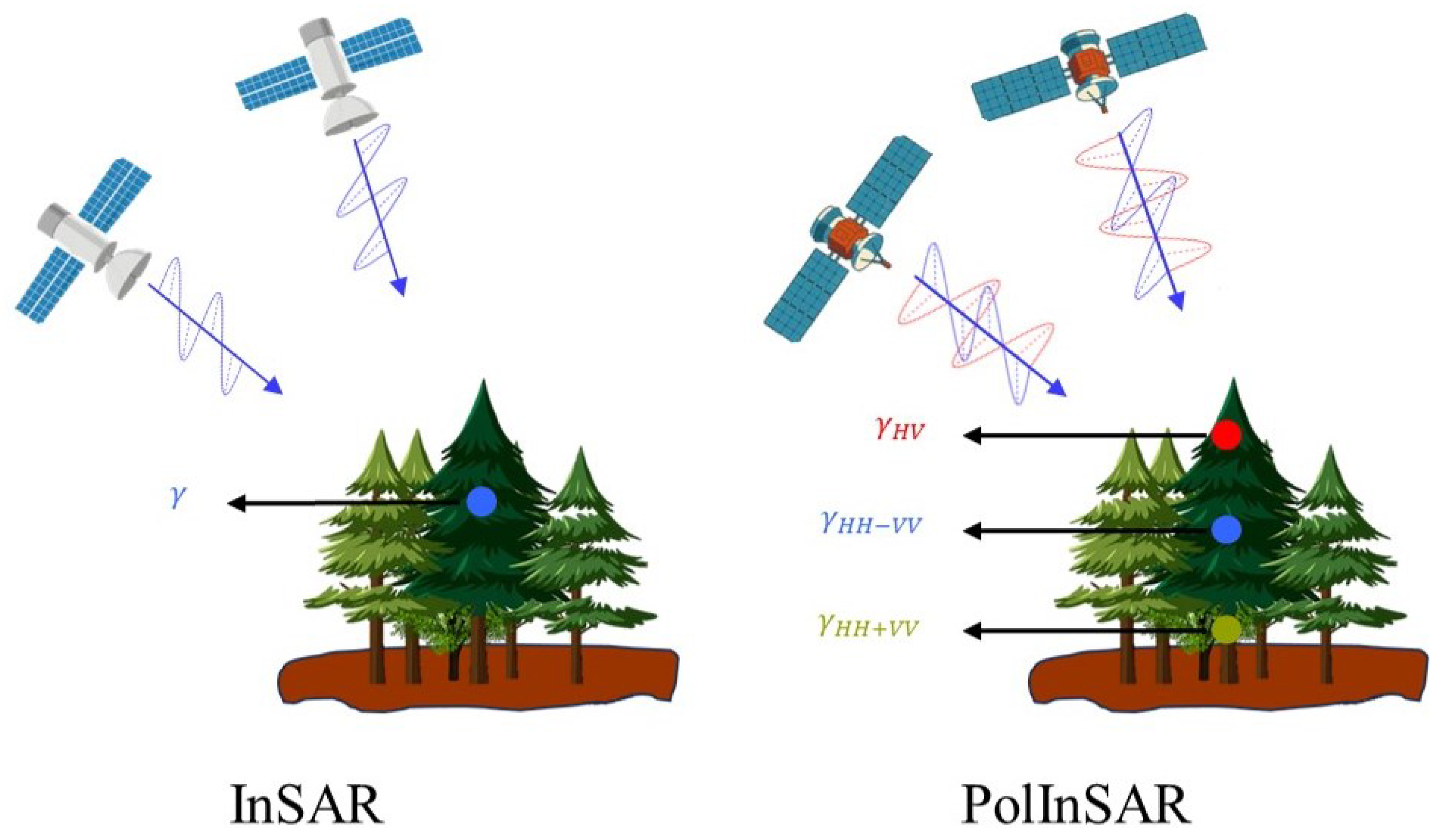
In recent years, spaceborne PolInSAR has been widely applied in forest parameter inversion [21,22,23,24]. In particular, L-band PolInSAR, with its strong penetration capability and sensitivity to ground surface information, has shown great potential for terrain mapping and structural inversion in forested areas. PolInSAR is an extension of InSAR technology [25,26]. It can distinguish different scattering centers corresponding to mixed scattering mechanisms occurring within the same resolution cell [27], thereby determining the heights of different media layers within the coverage layer, as shown in Figure 1. However, traditional PolInSAR inversion methods typically rely on simplified models, such as the random volume over ground (RVoG) model [28,29], which assumes a homogeneous volume structure and ideal ground return. In practice, factors such as temporal decorrelation, system noise, and baseline selection can significantly degrade inversion accuracy [30]. As a result, the rich information embedded in polarimetric data is not fully exploited, limiting further improvements in PolInSAR accuracy in complex terrain and forested areas.

In summary, a single data source is insufficient to meet the requirements of high-precision, long-term, and large-scale terrain modeling. Spaceborne LiDAR provides sparse but highly accurate ground measurements, while spaceborne PolInSAR offers wide-area and relatively high-resolution coverage capable of capturing continuous three-dimensional structural information, but its accuracy is constrained by model assumptions and noise. The two data sources are therefore complementary, and how to effectively integrate them to improve DEM accuracy in forested regions has become an urgent issue to be addressed.

Recently, deep learning has emerged as a powerful tool to address the limitations of traditional methods, particularly in nonlinear modeling and feature representation. However, the research on PolInSAR-based sub-canopy terrain inversion using deep learning remains relatively scarce. Some studies have explored the integration of deep learning with TomoPolSAR technology, employing coherence matrices as input features to design networks for estimating both vegetation height and sub-canopy terrain [31]. Although coherence matrices capture the polarization information in PolInSAR data and effectively model phase relationships between different polarization channels, achieving high-precision elevation reconstruction still heavily relies on radar geometric parameters. Ignoring this geometric information often leads to unreliable inversion results. Most research has concentrated on the inversion of vegetation height [32] and aboveground biomass [33]. For example, Zhang et al. [34] proposed the PolGAN method, which improves spatial resolution and vertical accuracy by integrating high-resolution PolInSAR data with low-resolution large-footprint LiDAR data. This method uses Generative Adversarial Networks (GANs) and dual discriminators that focus on coherence and spatiality. In fact, vegetation height and sub-canopy terrain share certain similarities in PolInSAR data as both are derived from the decomposition of PolInSAR scattering mechanisms. Consequently, the existing methods for vegetation height inversion offer valuable insights and serve as useful references for sub-canopy terrain inversion.

In order to fully exploit the vertical information provided by spaceborne PolInSAR in forest scenarios, this paper proposes a deep learning-based workflow and designs a PolInSAR and Spaceborne LiDAR Regression/Classification Network (PSLRC-Net). This method combines spaceborne PolInSAR data with sparse spaceborne LiDAR data to refine external DEMs and produce high-quality DEMs. To address the accuracy differences among the existing open DEMs in forested and non-forested areas, a binary forest/non-forest classification labeling approach is introduced. This approach guides the model to focus on these two regions separately, effectively improving the prediction accuracy in different areas. Specifically,

1.

Data fusion: We propose a deep learning-based workflow for integrating spaceborne PolInSAR and sparse spaceborne LiDAR data to provide an effective solution to the challenge of high-precision reconstruction in forested areas during DEM inversion. This workflow fully exploits the complementarity of multiple data sources and combines data-driven learning methods to significantly improve the model’s predictive capability in complex terrain and topographic reconstruction.

2.

Forest/non-forest labeling: To improve model performance in forested and non-forested areas, this paper proposes a lightweight binary classification method. By combining the accuracy differences of external DEMs in forested and non-forested areas with PolInSAR features, this method can automatically label forested and non-forested areas, thereby optimizing the processing workflow and significantly reducing computational costs.

3.

Region-specific optimization: We propose PSLRC-Net, a multi-task learning network that incorporates a forest/non-forest classification branch into the elevation inversion task to guide region-specific optimization of the model. This mechanism combines classification and regression tasks, directs the model to focus on feature differences between regions, adaptively optimizes the feature learning process, and significantly improves the accuracy of elevation prediction in forested and non-forested areas.

In summary, PSLRC-Net provides an innovative solution that effectively achieves accurate extrapolation of sparse spaceborne LiDAR footprint points through deep learning techniques and multi-source data fusion. It demonstrates high accuracy and adaptability, particularly in applications involving forested and non-forested areas. The code is available at: https://github.com/Liiiiiixs/PSLRC-Net (accessed on 20 September 2025).

The rest of this paper is organized as follows. Section 2 introduces the basic information of the multi-source data used in this study and the details of the study site. Section 3 provides a detailed description of the proposed method. Section 4 presents and analyzes the experimental results. Section 5 discusses the proposed methods. Finally, the conclusion is outlined in Section 6.

2. Study Site and Data

This section presents basic information about the study site and provides a systematic description of the multi-source data used, including their sources, characteristics, and specific applications in the research, thus providing strong data support for the study.

2.1. Study Site

This study performs experimental validation on data from two geographic sites, as shown in Figure 2.

The first site is located at the intersection of Luxembourg, Germany, France, and Belgium (${49}^{\circ }{18}^{\prime }$–${50}^{\circ }{02}^{\prime }$N, $5^{\circ }{42}^{\prime }$–$6^{\circ }{46}^{\prime }$E), with elevations ranging from approximately 130 m to 560 m above sea level (ASL). Since most of the area lies within Luxembourg, we refer to this site as LU. The northern part of this region is predominantly hilly. The central and southern parts are relatively flat, consisting of low hills and plains. Forested areas are distributed in distinct patches with well-defined boundaries.

The second site is on the border between Slovakia and Hungary (${48}^{\circ }{08}^{\prime }$–${48}^{\circ }{53}^{\prime }$N, ${19}^{\circ }{43}^{\prime }$–${20}^{\circ }{46}^{\prime }$E), with elevations ranging from approximately 100 m to 1400 m ASL. We refer to this site as SK. The northern and eastern parts of this region consist mainly of hills and mountains, characterized by significant topographic variations and extensive forest cover. The central and southern parts are dominated by plains and low hills, with relatively flat terrain. In contrast to the LU, forests here are more continuous and densely concentrated, with greater variations in elevation.

2.2. Spaceborne PolInSAR Data

Paired dual-polarization SAR data for interferometry were acquired by the SAOCOM-1B satellite under repeat-pass conditions with channels VH and VV. The SAOCOM-1B satellite is equipped with an L-band SAR operating at a frequency of approximately 1275 MHz, with a spatial resolution of about 3.75 m × 3.70 m. The spatial baselines for the LU and SK are 900.51 m and 516.94 m, respectively, and the temporal baselines are 31 days and 16 days, respectively. These data provide critical information support for analyzing regional surface characteristics.

2.3. Airborne LiDAR Data

The DEMs used for evaluation in this study were obtained from airborne LiDAR scans conducted in two regions, including Luxembourg (https://data.public.lu/en/datasets/bd-l-mnt5/) (accessed on 20 September 2025) and Slovakia (https://rpi.gov.sk/metadata/805fb72a-4132-4cd7-944a-88b8b2a7e6ed) (accessed on 20 September 2025).

The acquisition of airborne LiDAR-derived DEM (AL-DEM) data in Luxembourg began in February 2019, covering the entire geographic area of the country. The data have an average point density of approximately 15 points per square meter. The horizontal accuracy of the data is within ±3 cm, and the vertical accuracy is within ±6 cm.

The collection of Slovakia AL-DEM data was scheduled during the vegetation-free season. The last-return point density is at least 5 points per square meter, with one transverse swath per flight mission and a 20% overlap between swaths. The vertical accuracy of the point cloud is $m_h\le$ 0.11 m, and the horizontal position accuracy is $m_{xy}\le$ 0.30 m.

2.4. Spaceborne LiDAR Data

2.4.1. ICESat-2 Dataset

The ATL08 ($h\text{\_}te\text{\_}best\text{\_}fit$) product from the ICESat-2 (https://nsidc.org/data/atl08/versions/6) (accessed on 20 September 2025) satellite serves as the primary input for deep learning-based mapping. This specialized laser altimetry dataset is designed to measure terrain and vegetation, providing key parameters such as ground elevation and canopy height. The $h\text{\_}te\text{\_}best\text{\_}fit$ represents the terrain elevation at the midpoint of each 100 m segment, obtained from the best polynomial fit to ground photons, and is recommended as the most robust estimate of terrain elevation in ATL08. It provides a spatial resolution of approximately 100 m along the orbital track and a vertical measurement accuracy of centimeters, allowing for the capture of very fine variations in terrain and vegetation height [35]. We use the $h\text{\_}te\text{\_}uncertainty$ parameter from the ICESat-2 data to characterize data quality, and exclude footprints with $h\text{\_}te\text{\_}uncertainty>90$. For anomalous data that cannot be effectively identified using this parameter alone, we further apply filtering based on an external DEM (TanDEM-X): footprints are removed if the elevation difference with the external DEM is less than −5 m or greater than 40 m.

2.4.2. GEDI Dataset

The L2A ($elev\text{\_}lowestmode$) product from GEDI (https://search.earthdata.nasa.gov/search) (accessed on 20 September 2025) serves as the primary input for deep learning-based mapping. It provides detailed data on ground elevation and vegetation height, with individual laser footprints approximately 25 m in diameter. Vertical measurement accuracy ranges from a few centimeters to just over a dozen centimeters at the sub-meter level [36]. We extract parameters from the GEDI L2A data to characterize data quality, such as $quality\text{\_}flag$, $degrade\text{\_}flag$, and $sensitivity$. These parameters are then used for screening the GEDI data, retaining footprints that meet the criteria of $quality\text{\_}flag=1$, $degrade\text{\_}flag=0$, and $sensitivity>0.95$. For anomalous data that cannot be effectively identified using the above parameters, we also apply a filtering strategy based on an external DEM (TanDEM-X): footprints are excluded if their elevation difference from the external DEM is less than −5 m or greater than 40 m.

3. Methodology

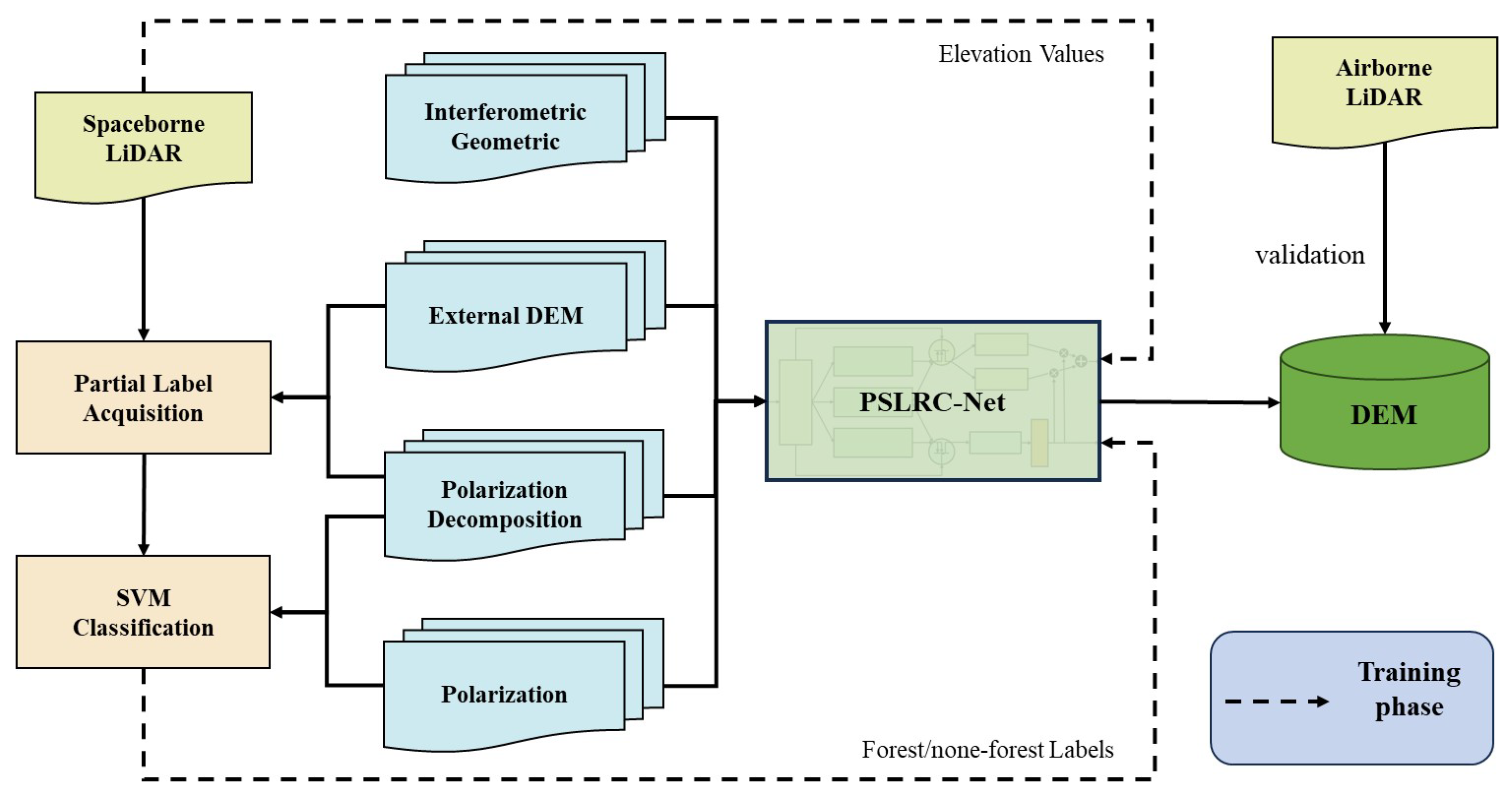
Figure 3 depicts the overall workflow of the proposed method. This section provides a detailed explanation of the selected features, the acquisition of classification labels, the structure of the PSLRC-Net, and the design of the loss function.

3.1. Feature Description

The features used in this study are categorized into four types: external DEM features, interferometric geometric features, polarization features, and polarimetric decomposition features, as shown in

Table 1. Features selected for PSLRC-Net training.

Feature	Description
External DEM
$h_{\mathrm{DEM}}$	TanDEM-X DEM
${\tau }_s$	Local Angle
Interferometric Geometric
$k_z$	Interferometric Vertical Wavenumber
${\varphi }_{\mathrm{topo}}$	Topographic Phase
Polarization
${\gamma }_{\mathrm{VH}}$	VH Channel Coherence
${\gamma }_{\mathrm{VV}}$	VV Channel Coherence
Polarimetric Decomposition
H	Entropy of the $H/\alpha$ Decomposition
$\alpha$	Mean Scattering Angle of the $H/\alpha$ Decomposition
$|{\sigma }_{\mathrm{VH}}|$	VH Backscatter
$|{\sigma }_{\mathrm{VV}}|$	VV Backscatter

. External DEM features use TanDEM-X (https://download.geoservice.dlr.de/TDM30_EDEM/) (accessed on 20 September 2025) data and local angle information to provide an elevation reference for the algorithm. Interferometric geometric features are related to satellite observation parameters and are used to describe the geometric structure of interferometric signals, where

$$k_z=m{\displaystyle \frac{2\pi }{\lambda }}{\displaystyle \frac{B_{\perp }}{Rsin{\theta }_0}}.$$

(1)

The coefficient m represents the acquisition mode: $m=2$ for monostatic acquisition and $m=1$ for bistatic acquisition. $B_{\perp }$ is the perpendicular baseline, $\lambda$ is the radar wavelength, R is the slant range, and ${\theta }_0$ is the local incidence angle. Using the $h_{\mathrm{DEM}}$ and $k_z$, we can obtain

$${\varphi }_{\mathrm{topo}}=\mathrm{wrap}\left(k_z·h_{\mathrm{DEM}}\right)$$

(2)

where $\mathrm{wrap}(·)$ denotes the phase wrapping operation, which typically restricts the phase to the range $(-\pi ,\pi ]$. This topographic phase can serve as a reference for the interferometric phase, providing prior information for subsequent processing.

The latter two polarization-related features are based on dual-polarization data. Under usual assumptions of ergodicity and stationarity, a $4\times 4$ covariance matrix can be constructed using the two polarization channels from the master and slave images:

$$\mathbf{C}=〈\left[\begin{array}{c}{\mathbf{k}}_1\\ {\mathbf{k}}_2\end{array}\right]\left[\begin{array}{cc}{\mathbf{k}}_1^H& {\mathbf{k}}_2^H\end{array}\right]〉=\left[\begin{array}{cc}{\mathbf{C}}_1& \mathbf{\Omega }\\ {\mathbf{\Omega }}^H& {\mathbf{C}}_2\end{array}\right]$$

(3)

where ${\mathbf{k}}_i={\left[\begin{array}{c}{\sigma }_{{\mathrm{VH}}_i},{\sigma }_{{\mathrm{VV}}_i}\end{array}\right]}^T,i=1,2$ is the scattering vector; ${\sigma }_{{\mathrm{VH}}_i}$ and ${\sigma }_{{\mathrm{VV}}_i}$ are the complex scattering coefficients. ${(·)}^H$ represents the conjugate transpose, and $\langle ·\rangle$ represents the average operation in data processing.

For any given non-zero scattering mechanism $\omega$, the complex interferometric coherence can be expressed as

$${\gamma }_{\omega }={\displaystyle \frac{{\omega }^H\mathbf{\Omega }\omega }{{\omega }^H\mathbf{C}\omega }}$$

(4)

where $\mathbf{C}=({\mathbf{C}}_1+{\mathbf{C}}_2)/2$. In this study, the coherence of the VH and VV bases generated by ${\omega }_1={\left[\begin{array}{cc}1& 0\end{array}\right]}^T$ and ${\omega }_2={\left[\begin{array}{cc}0& 1\end{array}\right]}^T$ were selected as input features.

By performing an eigendecomposition on the covariance matrix C [37], we obtain

$$\mathbf{C}=\sum _{i=1}^2{\lambda }_i{\mathbf{e}}_i{\mathbf{e}}_i^{\mathbf{H}}$$

(5)

where ${\lambda }_i$ denotes the i-th eigenvalue of the matrix $\mathbf{C}$, and ${\mathbf{e}}_i$ is the normalized eigenvector corresponding to ${\lambda }_i$. The normalized eigenvalue ratio is defined as

$$p_i={\displaystyle \frac{{\lambda }_i}{{\sum }_{j=1}^2{\lambda }_i}}.$$

(6)

Then, the entropy H and mean scattering angle $\alpha$ of the $H/\alpha$ decomposition are calculated as

$$\begin{array}{cc}\hfill H& =-\sum _{i=1}^2{p}_i{log}_2{p}_i\hfill \\ \hfill \alpha & =\sum _{i=1}^2{p}_{i}arccos\left(\left|{\mathbf{e}}_{i1}\right|\right)\hfill \end{array}$$

(7)

where $|{\mathbf{e}}_{i1}|$ represents the magnitude of the first element of the eigenvector ${\mathbf{e}}_i$. Finally, $|{\sigma }_{\mathrm{VH}}|$ and $|{\sigma }_{\mathrm{VV}}|$ can be obtained by averaging the backscatter coefficient magnitudes of the master and slave images.

3.2. Classification Label Acquisition

For the training requirements of the PSLRC-Net classification branch, this paper proposes an efficient method for obtaining forest and non-forest labels. The method consists of two steps: In the first step, we acquire a portion of accurate and easily accessible labeled data. In the second step, we combine these labeled data with other features to train a support vector machine (SVM) model, which is then used to label the data points that are difficult to classify in the first step. Ultimately, this approach allows classification of the entire spaceborne LiDAR footprint.

3.2.1. Step 1: Initial Labeling

This study found that the external DEM obtained from InSAR data using traditional methods has high accuracy in non-forested areas but shows significant overestimation in forested areas (Table 4 provides a vertical accuracy assessment of TanDEM data in different areas). In addition, the $H/\alpha$ decomposition of PolSAR data can also provide information for the forest/non-forest binary classification due to its sensitivity to the scattering mechanisms in the scene. Specifically, the ground scattering mechanism is relatively simple, mainly surface scattering, with low uncertainty, leading to lower H and $\alpha$ values, while the forest scattering mechanism is more complex and uncertain, leading to higher H and $\alpha$ values.

Using the elevation difference along with the polarization $H/\alpha$ decomposition, we can represent spaceborne LiDAR footprint point as a three-dimensional vector. The entire set of data points can be represented as $\mathbf{X}=\{(\Delta z_i,h_i,{\alpha }_i)\mid i=1,2,\dots ,N\}$, where $\Delta z_i$ represents the elevation difference between the external DEM and the spaceborne LiDAR elevation, $h_i$ and ${\alpha }_i$ represent the $H/\alpha$ decomposition values for that point, and N is the number of spaceborne LiDAR footprint points. Using the K-means clustering algorithm [38], the data can be divided into three categories:

$$\mathbf{X}\stackrel{\mathrm{K}\text{-}\mathrm{Means}}{\to }\{{\mathbf{X}}_1,{\mathbf{X}}_2,{\mathbf{X}}_3\}$$

(8)

where ${\mathbf{X}}_j=\{x_i\in \mathbf{X}\mid y_i=j\}$, ${\mathbf{X}}_j$ represents the subset of data points belonging to the j-th class, and $y_i\in \{1,2,3\}$ is the class label for each data point.

Among these three categories, the first class represents the ground, characterized by low elevation difference, low entropy, and low $\alpha$; the second class represents the forest, characterized by high elevation difference, high entropy, and high $\alpha$; and the third class represents other areas, characterized by low elevation variation, high entropy, and high $\alpha$. By eliminating outliers that are far from the cluster centers in each class and removing data points from the “other” class, we can extract a subset of high-confidence labels.

3.2.2. Step 2: Classification Label of Spaceborne LiDAR Footprints

By combining the extracted high-confidence labeled data with other features, we can obtain a classified dataset $\mathcal{D}=\{({\mathbf{x}}_1,y_1),({\mathbf{x}}_2,y_2),\dots ,({\mathbf{x}}_N,y_N)\}$, where

$$\begin{array}{cc}\hfill {\mathbf{x}}_i& =[{\gamma }_{VH}^i,{\gamma }_{VV}^i,H^i,{\alpha }^i,|{\sigma }_{\mathrm{VH}}^i|,|{\sigma }_{\mathrm{VV}}^i\left|\right]\hfill \\ \hfill y_i& =\left\{\begin{array}{c}1,\mathrm{Forest}\hfill \\ -1,\mathrm{non}\text{-}\mathrm{Forest}\hfill \end{array}\right.\hfill \end{array}$$

(9)

Considering the limited number of samples and their sparse distribution, this study employs the SVM [39] as the classifier. SVM demonstrates strong generalization ability under small-sample conditions, allowing it to establish a stable classification hyperplane with limited high-confidence samples. Meanwhile, its low computational cost makes it suitable for rapid and effective initial binary classification in the case of sparse spaceborne LiDAR footprints. The optimization objective can be expressed as

$$\begin{array}{cc}\hfill & \underset{\mathbf{w}}{min}\left({\displaystyle \frac{1}{2}}{\parallel \mathbf{w}\parallel }^2\right)\hfill \\ \hfill \mathrm{subject}\mathrm{to}& y_i(\mathbf{w}·{\mathbf{x}}_i+b)\ge 1,i=1,\dots ,N\hfill \end{array}$$

(10)

where $\mathbf{w}$ is the weight vector perpendicular to the hyperplane, and b is the bias term. By training on this dataset, classification labels can be generated for the entire spaceborne LiDAR footprint.

3.3. PSLRC-Net

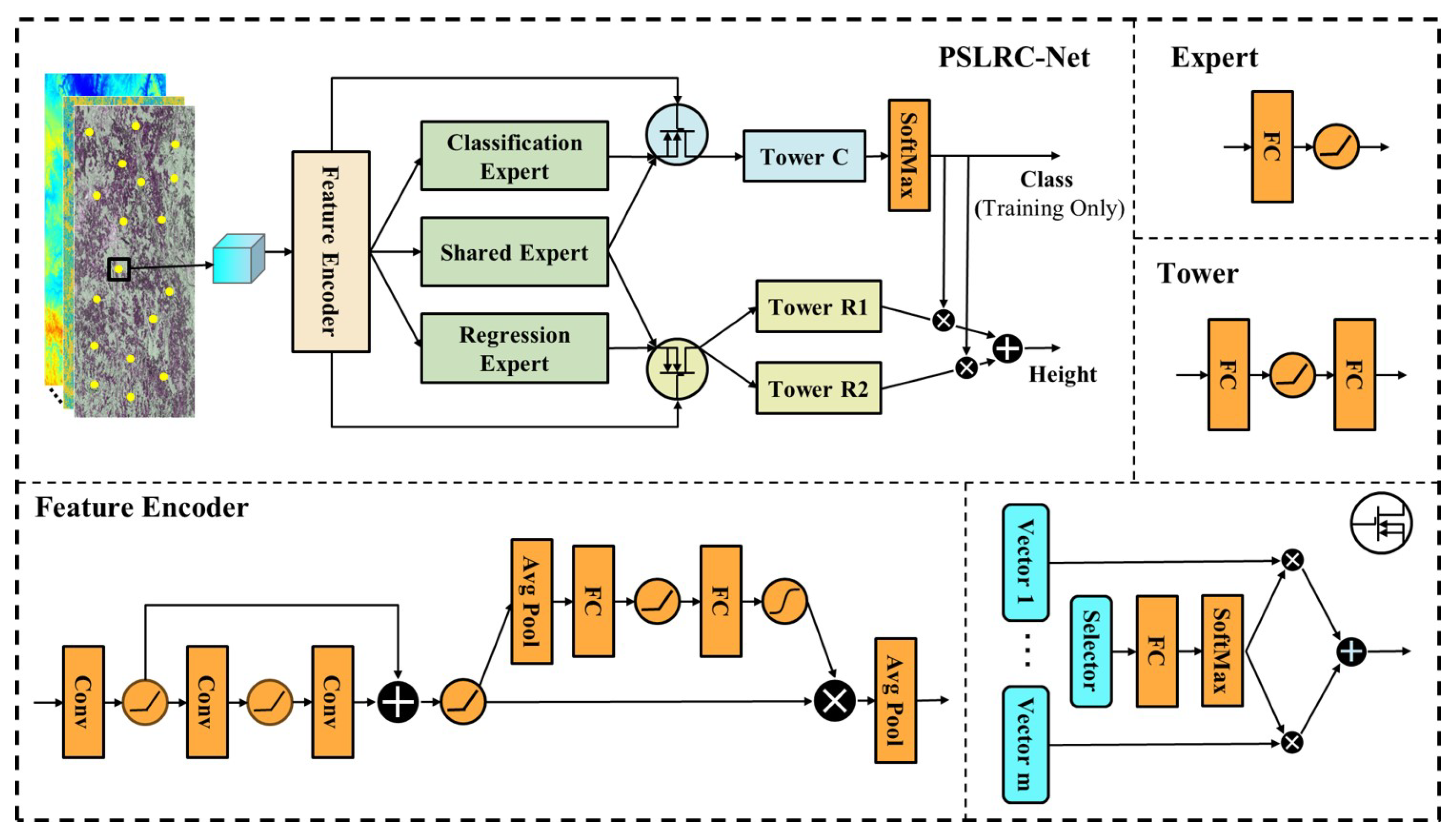
The structure of PSLRC-Net is shown in Figure 4. The network first extracts feature cubes from the positions of spaceborne LiDAR footprint points, which are then processed through a feature encoder, expert network, and task processing module, ultimately outputting highly accurate classification results and elevation predictions.

The feature encoder layer consists of a convolutional neural network (CNN), residual blocks (ResBlock), Squeeze-and-Excitation blocks (SEBlock), and an average pooling layer. The role of this part is to extract multi-scale multi-level feature information from the input data.

The core of the network is based on the Multi-gate Mixture of Experts (MMoE) [40] and Customized Gate Control (CGC) [41] methods using a gate network-based expert selection mechanism. This mechanism dynamically selects shared and task-specific experts based on task requirements. Through gating, the network adaptively adjusts the contribution of experts for different branches (regression and classification) to optimize task performance. Specifically, the feature $\mathbf{x}$ obtained from the feature encoder is processed through the shared expert layers and the task-specific expert layers, yielding the corresponding latent representations:

$${\mathbf{h}}_e^i=f_e^i\left(\mathbf{x}\right),i=1,2,...,N_e$$

(11)

where $e\in \{s,r,c\}$ represents the shared experts, regression experts, and classification experts, respectively, and $N_e$ denotes the number of experts in each category.

For task $t\in \{r,c\}$, the gating network generates task-specific weights:

$${\mathbf{G}}_t=\mathrm{Softmax}({\mathbf{W}}_t\mathbf{x}+{\mathbf{b}}_t)$$

(12)

where ${\mathbf{W}}_t$ and ${\mathbf{b}}_t$ are the parameters of the gating network for task t, and ${\mathbf{G}}_t$ represents the weights assigned to both shared and task-specific experts. Finally, the output weighted by the gating network can be expressed as

$${\mathbf{H}}_t=\sum _{j=1}^{N_s}{\mathbf{G}}_{t,j}{\mathbf{h}}_j^s+\sum _{k=1}^{N_t}{\mathbf{G}}_{t,N_s+k}{\mathbf{h}}_k^t.$$

(13)

In this way, each task t can adaptively select and aggregate outputs from both shared and task-specific experts, effectively optimizing its learning objectives.

The task processing module consists of a regression branch and a classification branch, with the regression branch composed of two task towers, and their outputs are expressed as

$${\widehat{\mathbf{y}}}_r^i=f_{\mathrm{reg}}^i\left({\mathbf{H}}_r\right),i=1,2.$$

(14)

The classification branch adjusts the shared layer parameters together with the regression tasks through multi-task learning, providing additional supervision signals to the regression tasks. The output of the classification branch is

$${\widehat{\mathbf{y}}}_c=f_{\mathrm{cls}}\left({\mathbf{H}}_c\right).$$

(15)

In addition, the classification branch weights the outputs of the regression task towers, allowing the network to adaptively focus on feature differences in different regions, especially in forested areas, thereby improving the accuracy of regression predictions. The final regression output can be expressed as

$${\widehat{\mathbf{y}}}_r={\widehat{\mathbf{y}}}_c·{\widehat{\mathbf{y}}}_r^1+(1-{\widehat{\mathbf{y}}}_c)·{\widehat{\mathbf{y}}}_r^2.$$

(16)

3.4. Loss Function

The training loss of PSLRC-Net consists of a regression loss and a classification loss. The regression loss is calculated using the Mean Squared Error (MSE),

$${\mathcal{L}}_{\mathrm{reg}}={\displaystyle \frac{1}{N}}{\parallel {\mathbf{y}}_r-{\widehat{\mathbf{y}}}_r\parallel }^2={\displaystyle \frac{1}{N}}\sum _{i=1}^N{\left(y_{ri}-{\widehat{y}}_{ri}\right)}^2$$

(17)

where ${\mathbf{y}}_r$ represents the ground truth values for the regression task, which are the spaceborne LiDAR elevation values; ${\widehat{\mathbf{y}}}_r$ is the predicted value output by the network, as shown in Equation (16); and N is the number of samples.

The classification loss is calculated using Cross-Entropy Loss,

$${\mathcal{L}}_{\mathrm{cls}}=-{\displaystyle \frac{1}{N}}\sum _{i=1}^N\sum _{j=1}^2{y}_{cij}log\left({\widehat{y}}_{cij}\right)$$

(18)

where $y_{cij}$ represents the ground truth labels, and ${\widehat{y}}_{cij}$ is the predicted probability.

Directly summing these two losses with simple weighting may lead to an inappropriate weight distribution during training, which could negatively affect model performance. On the one hand, there are inherent differences in the optimization objectives between the regression and classification tasks. On the other hand, differences in data distribution and convergence speed between the tasks can cause one task to dominate the total loss, thus limiting the full optimization of the other task. To address the above issues, we adopted a weighted loss function design based on task uncertainty. This method is not only theoretically interpretable but also allows for dynamic adjustment of the relative weights of the multi-task losses, thereby better coordinating the joint optimization of the regression and classification tasks. Specifically, the training loss function is defined as [42]

$$\mathcal{L}={\displaystyle \frac{1}{2{\sigma }_{\mathrm{r}}^2}}{\mathcal{L}}_{\mathrm{reg}}+{\displaystyle \frac{\lambda }{2{\sigma }_{\mathrm{c}}^2}}{\mathcal{L}}_{\mathrm{cls}}+log\left(1+{\sigma }_{\mathrm{r}}^2\right)\left(1+{\sigma }_{\mathrm{c}}^2\right)$$

(19)

where ${\sigma }_{\mathrm{r}}$ and ${\sigma }_{\mathrm{c}}$ are learnable parameters associated with task uncertainty. Their physical meaning is to capture the noise level of the different tasks. Specifically, a larger $\sigma$ indicates higher uncertainty for the corresponding task, thereby dynamically reducing its loss weight. Conversely, a smaller $\sigma$ increases the relative importance of the task, encouraging the model to allocate more learning capacity to the more reliable task. In addition, the regularization term $log\left(1+{\sigma }^2\right)$ is introduced to not only effectively prevent the unbounded contraction or expansion of ${\sigma }_{\mathrm{r}}$ and ${\sigma }_{\mathrm{c}}$ but also to ensure the non-negativity of the loss function, thereby improving the numerical stability and training robustness of the model.

Due to the large difference between the regression loss and the classification loss, a factor $\lambda$ is introduced, which can be set based on the initial ratio ${\mathcal{L}}_{\mathrm{reg}}/{\mathcal{L}}_{\mathrm{cls}}$. The purpose of this factor is to adjust the classification and regression losses to the same scale.

4. Results

We validated PSLRC-Net through experiments with spaceborne PolInSAR data. The quantity and quality of the spaceborne LiDAR data at the two sites are summarized in

Table 2. Spaceborne LiDAR data quantity and quality.

Site	LiDAR	Total	Proportion			RMSE (m)
			All	Forest	Ground
LU	ICESat-2	78,278	0.11%	0.08%	0.14%	2.32
	GEDI	210,718	0.30%	0.34%	0.25%	5.30
SK	ICESat-2	136,621	0.11%	0.10%	0.17%	2.21
	GEDI	459,967	0.39%	0.56%	0.34%	5.72

, with the RMSE derived using AL-DEM as the baseline. Unless otherwise noted, the ground truth data in our experiments are derived from ICESat-2, and the reference DEM is based on TanDEM data. The impact of the GEDI dataset is analyzed in detail in Section 5.1, focusing on how data quality and quantity affect the experimental results. The impact of different reference DEMs on the experimental results is further analyzed in Section 5.2, where we evaluate how the choice of reference data affects the accuracy of DEM generation.

During data preprocessing, we standardized the features to improve numerical stability during model training. Specifically, before windowing, we first computed the mean and standard deviation for each feature across the entire data range shown in Table 1 and normalized each feature based on these values. This approach ensures consistent scaling of the features across the entire dataset, thereby avoiding any potential bias that could result from normalization within each window. The spaceborne LiDAR footprint points were divided into a training set and a test set, with 80% of the data used for training and 20% for testing.

4.1. Binary Classification Performance Assessment

This section presents the output results of the PSLRC-Net classification branch to evaluate its effectiveness in the classification task. For the visualization of dual-polarization data, we used a lexicographic basis instead of the Pauli basis, and used a color combination similar to Pauli RGB: the R channel represents the magnitude of the VV channel, the G channel represents the magnitude of the VH channel, and the B channel represents the magnitude of the VV channel. This visualization method is called pseudo-Pauli RGB.

Figure 5a shows the clustering results of all the footprint points from the LU in a 3D coordinate system composed of elevation difference, H, and $\alpha$. The spatial distribution of the clustering results in the pseudo-Pauli RGB is shown in Figure 5b. For clarity, we have chosen a subset of the LU. It can be seen that the “Ground” and “Forest” data points perform well in their respective areas, while the “Other” data points appear not only in the ground area but also in parts of the forested area. After excluding the “other” category, a set of accurate labeled data is obtained. By using this labeled data to train the SVM model, the classification results of all spaceborne LiDAR footprints can be obtained, and their spatial distribution is shown in Figure 5c. These classification labels can be used to further train PSLRC-Net.

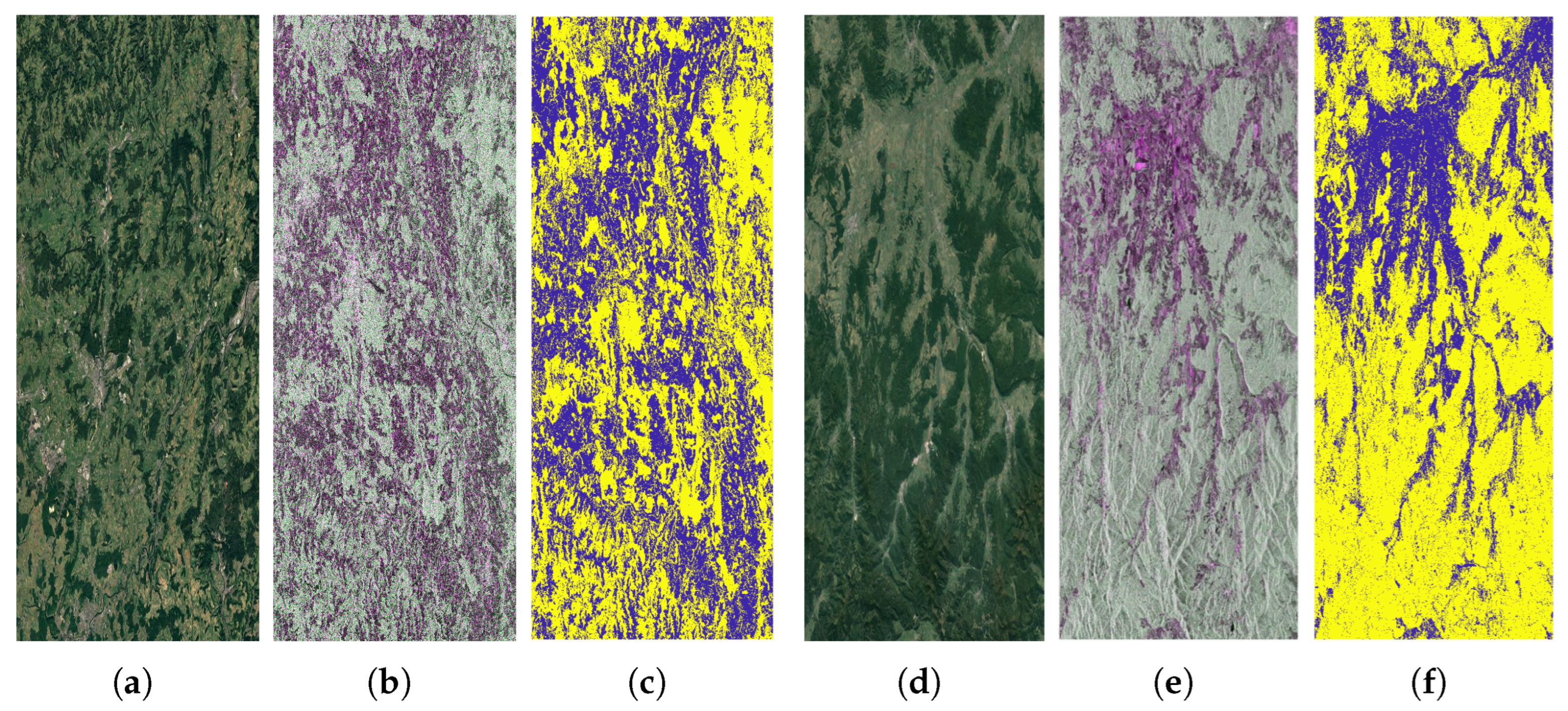
Figure 6 shows the output of the classification branch of PSLRC-Net for the two test sites. The optical imagery from Google Earth and the pseudo-Pauli RGB images partially reflect the distribution of forested and non-forested areas and can serve as references for validating the classification results. As shown in the figure, the classification results agree well with the distributions observed in the optical imagery and the pseudo-Pauli RGB images. This consistency demonstrates that the model effectively captures the distinctive features of different categories and uses these features for accurate classification, providing strong support for its performance in elevation inversion tasks.

For quantitative assessment, the classification accuracy on the test sets of the two sites reached 99.70% and 99.67%, respectively, demonstrating the high reliability of the classification branch.

4.2. Regression Performance Evaluation for PSLRC-Net

To evaluate the performance of PSLRC-Net in the regression prediction task, this section compares it to other methods. Traditional machine learning methods such as Random Forest (RF), XGBoost, Gradient Boosting Decision Tree (GBDT), K-Nearest Neighbor (KNN), and Support Vector Regression (SVR) have been widely applied in the inversion of forest parameters like tree height and aboveground biomass [43,44] through the fusion of PolInSAR and sparse LiDAR data. In contrast, deep learning techniques have seen more limited application in this field, especially in the inversion of understory DEMs. In this section, we compare these traditional methods with the PSLRC-Net approach.

Specifically, we use TanDEM data as a benchmark, train different methods on the same training set, and evaluate their performance differences on the test set. The results are presented in

Table 3. Performance assessment of various methods.

ID	Metric	TanDEM	Base Model		Ensemble Model			PSLRC
			KNN	SVR	RF	XGBoost	GBDT
LU	$R^2$	0.9915	0.9951	0.9954	0.9965	0.9966	0.9963	0.9979
	RMSE (m)	6.51	4.97	4.83	4.21	4.21	4.35	3.78
	MAE (m)	4.10	3.32	3.17	2.73	2.78	2.94	2.48
SK	$R^2$	0.9989	0.9994	0.9994	0.9995	0.9995	0.9995	0.9997
	RMSE (m)	8.68	6.09	6.14	5.21	5.76	5.77	4.91
	MAE (m)	6.16	4.22	4.29	3.47	3.76	4.06	3.36

.

Compared to the TanDEM dataset, all the algorithms show improvements in various metrics for the DEM regression task, but there are significant performance differences between the algorithms. The performance of KNN and SVR is relatively weak. Although these two algorithms can provide stable predictions to some extent, their overall performance in elevation inversion tasks is significantly inferior to the other methods. This may be due to their limited ability to model complex high-dimensional data patterns and handle nonlinear relationships. Ensemble learning algorithms such as RF, XGBoost, and GBDT show relatively high accuracy and stability. By combining the predictions of multiple base learners, these algorithms improve the generalization ability and prediction accuracy of the model, resulting in reasonably good performance in the height inversion task. In comparison, PSLRC-Net outperforms all the other methods on all the evaluation metrics. This indicates that PSLRC-Net has superior modeling capabilities for handling complex high-dimensional data patterns and is particularly well suited to the demands of elevation inversion tasks.

It should be noted that the $R^2$ values in Table 3 being close to 1 do not indicate model overfitting. This mainly results from the large elevation range of the study areas. By definition,

$$R^2=1-{\displaystyle \frac{{\sum }_{i=1}^n{(y_i-{\widehat{y}}_i)}^2}{{\sum }_{i=1}^n{(y_i-\overline{y})}^2}}$$

(20)

when the overall relief is large, the denominator becomes very large, and even meter-level residuals make the $R^2$ values close to 1. Thus, the high R²; reflects a terrain-scale effect rather than model overfitting. Meanwhile, the RMSE and MAE on independent test sets are significantly reduced compared with the baseline methods, which more directly reflect the prediction accuracy and generalization ability.

4.3. DEM Result Assessment

Based on the excellent performance of PSLRC-Net on the test set, this section uses PSLRC-Net to extrapolate the spaceborne LiDAR footprints to the entire area and validates the results using AL-DEM. The inversion results of the DEMs for the two sites are shown in Figure 7.

We compared the PSLRC DEM with several external DEMs, including ASTER GDEM, SRTM, AW3D30, TanDEM-X (sorted by acquisition time), and DEMs derived from the traditional RVoG model, all converted to the EGM96 [45] height reference. The three-stage inversion method of the traditional RVoG model suffers from the “double-candidate effect” [21], and dual-polarization data cannot utilize the different penetration depths of the scattering channels under the Pauli basis to select the terrain phase [46]. To solve this problem, we adopted the method proposed in Ref. [22] to obtain the RVoG model DEM, which effectively solves the terrain phase selection problem under dual-polarization data.

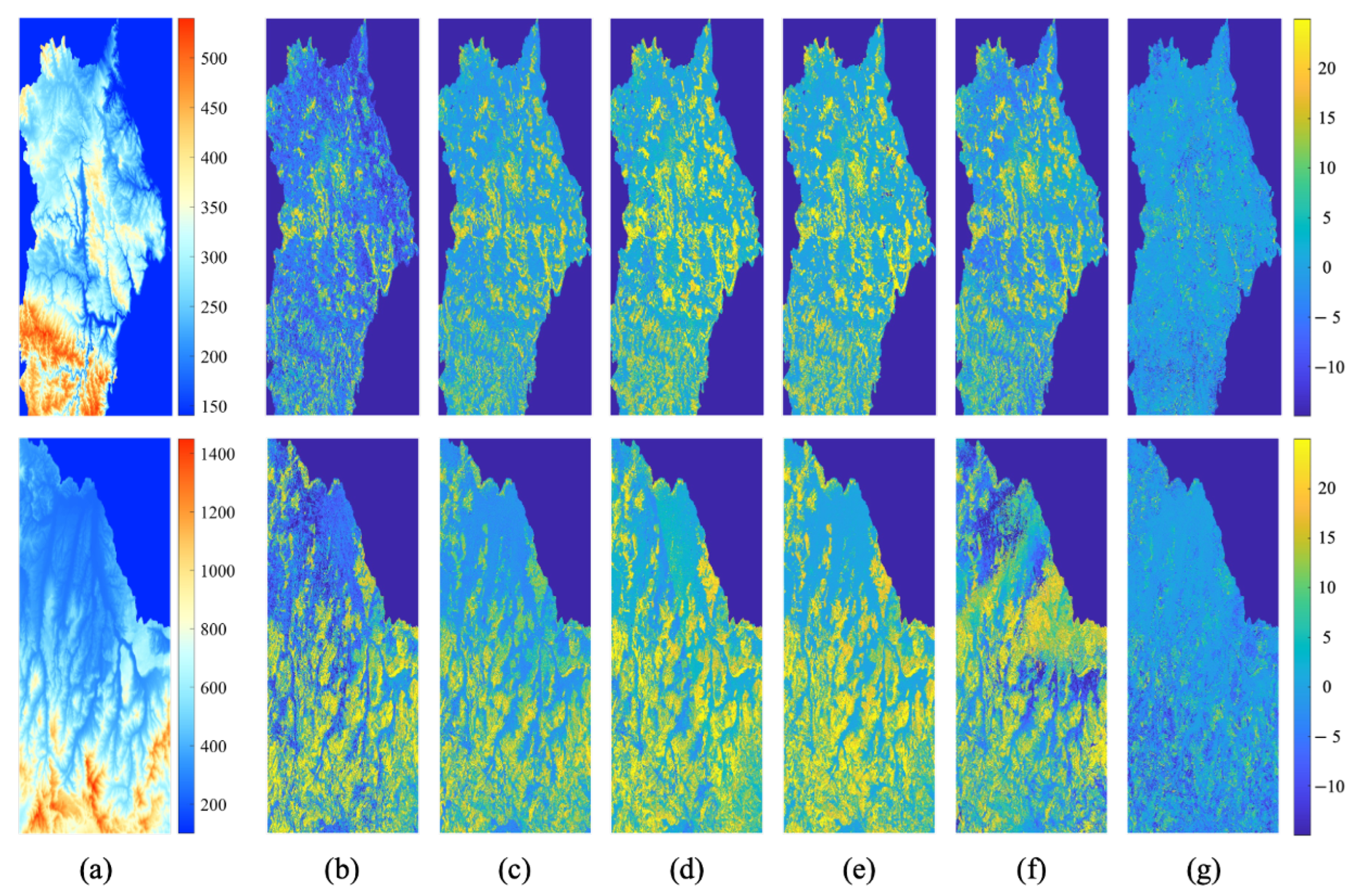
Considering the large range of DEM values, it is difficult to directly observe the differences between different DEMs. Therefore, this study presents the elevation differences between different DEMs and AL-DEM. Specifically, in the difference maps, the green areas near the zero value on the color bar indicate that the DEM is closer to the AL-DEM, while the yellow areas indicate that the DEM is higher relative to the AL-DEM. As shown in Figure 8, all the DEMs except the PSLRC DEM show significant differences from the AL-DEM. GDEM performs the worst, while the other DEM products show relatively consistent overall trends, generally overestimating elevations in forested areas. Among them, AW3D30 shows significant elevation discontinuities caused by regional stitching. Due to the low stability of the RVoG model inversion, the inversion results fail in some areas. In contrast, the PSLRC DEM is closer to the AL-DEM.

Based on the obtained classification map of the forested and non-forested areas, we used the AL-DEM to perform numerical assessments of the different areas within the two sites. The results are shown in

Table 4. Assessment of the elevation accuracy of different DEMs.

ID	DEM	All			Forest		Ground
		ME (m)	RMSE (m)	MAE (m)	RMSE (m)	MAE (m)	RMSE (m)	MAE (m)
LU	GDEM	−1.25	9.08	7.34	10.10	7.91	7.89	6.77
	SRTM	3.88	8.39	5.57	11.39	8.90	3.13	2.17
	AW3D30	6.81	11.43	7.47	15.56	12.38	4.11	2.46
	TanDEM	6.15	11.04	6.67	15.22	11.80	3.16	1.61
	RVoG	3.95	9.54	6.58	12.45	9.68	5.05	3.41
	PSLRC	0.03	4.05	2.48	5.41	3.94	1.82	1.00
SK	GDEM	4.60	13.32	10.49	14.56	11.62	9.62	7.70
	SRTM	5.45	10.07	7.39	11.62	9.16	4.30	3.02
	AW3D30	9.00	13.00	9.63	15.04	12.22	5.26	3.26
	TanDEM	9.12	13.01	9.34	15.28	12.52	4.03	1.84
	RVoG	5.93	11.81	9.11	12.97	10.19	8.31	6.45
	PSLRC	−0.39	4.84	3.29	5.59	4.23	2.07	0.98

. It is evident that the PSLRC DEM outperforms the other DEMs in all the metrics in different areas, with particularly significant improvements in forested areas. In the entire region, the RMSE decreased by 51.7–64.6% and 51.9–63.7% at the two sites, while the MAE decreased by 55.5–66.8% and 55.5–68.6%. In the forested areas, the RMSE decreased by 46.4–65.2% and 51.9–63.4%, and the MAE decreased by 50.2–68.2% and 53.8–66.2%. Even in land areas with relatively small errors, the PSLRC DEM still achieves high accuracy, demonstrating its reliability and precision in elevation inversion.

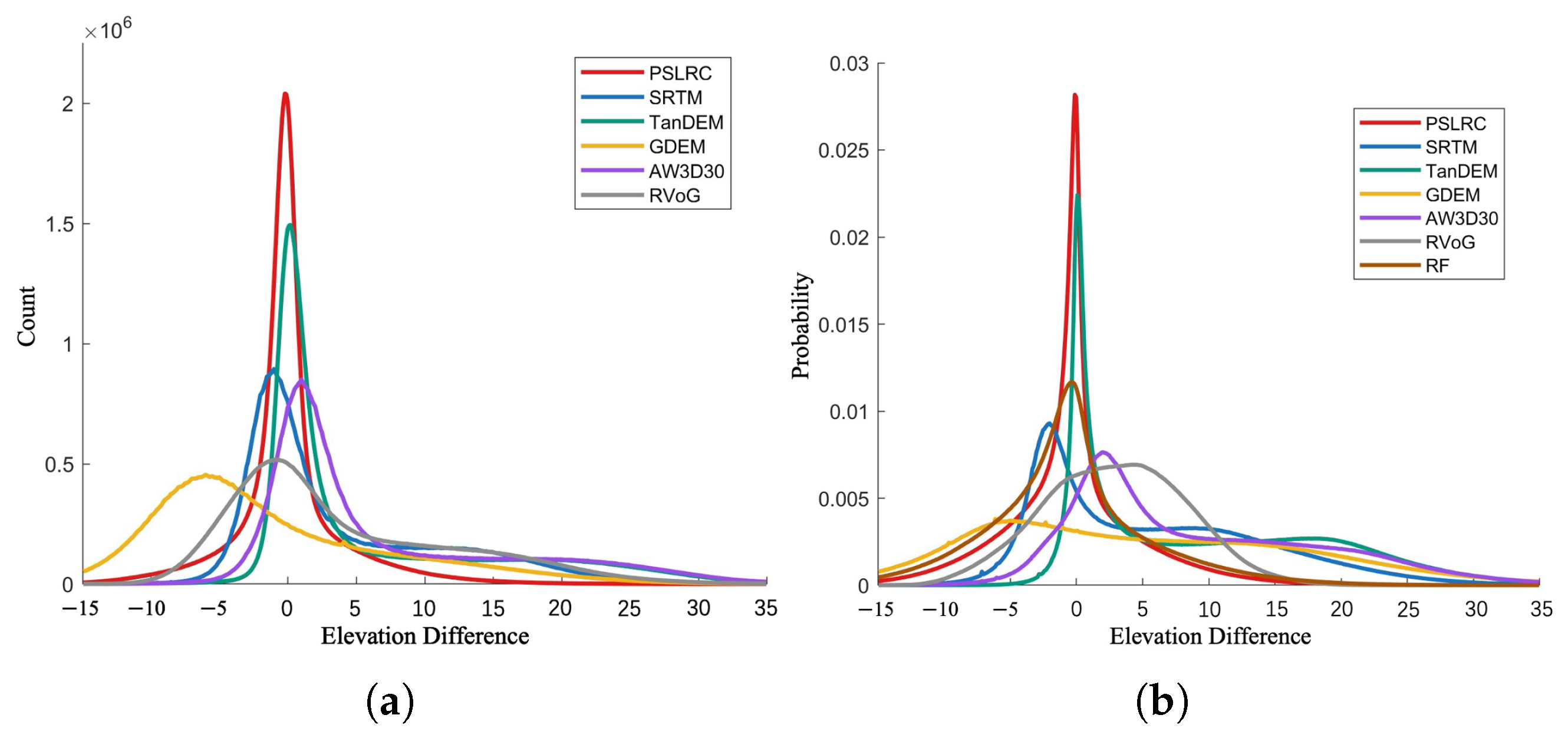
Comparing the difference histograms of the different DEMs with AL-DEM in Figure 9, it can be seen that GDEM is generally lower, while the SRTM and AW3D30 DEMs have similar distributions. The height difference of PSLRC DEM and TanDEM is close to zero, but, due to the overestimated heights in forested areas, TanDEM still shows a large distribution in regions with high height differences.

4.4. Ablation Study

To comprehensively understand the contribution of each component to the overall model performance, this study conducted ablation experiments to systematically evaluate the key modules of the model. Specifically, the core components were individually removed or replaced, followed by model retraining and DEM inversion. The regional accuracy of the model was then evaluated by comparison with the AL-DEM. Detailed results are presented in

Table 5. Ablation study results for PSLRC-Net.

ID	Metric	PSLRC	Module				Feature
			FE	EM	CH	ORT	IG	Pol	PDec
LU	RMSE (m)	4.05	4.37	4.22	4.21	4.26	4.28	4.27	5.19
	MAE (m)	2.48	2.71	2.59	2.56	2.66	2.64	2.62	3.33
SK	RMSE (m)	4.84	5.34	4.97	5.07	4.98	5.07	5.16	5.41
	MAE (m)	3.29	3.68	3.44	3.51	3.42	3.49	3.58	3.74

Note: FE stands for feature encoder, EM stands for expert mechanism, CH stands for classification head, ORT stands for one regression tower, IG stands for interference geometry features, Pol stands for polarization features, and PDec stands for polarimetric decomposition features.

.

The table sequentially lists models with the ablation of the feature encoder (FE), expert mechanism (EM), classification head (CH), one regression tower (ORT), as well as interference geometry features (IG), polarization features (Pol), and polarimetric decomposition features (PDec). The objective of this analysis is to assess the impact of each module or feature on the overall performance of the model.

In the module ablation study, removing the feature encoder resulted in a significant decrease in model accuracy, highlighting its critical role in feature extraction. The classification head and the dual regression towers form the core of the multi-task structure. The ablation experiments showed that removing the classification head or using a single regression tower significantly affected performance, demonstrating that the multi-task structure effectively enhances the model’s ability to learn complex regional features, thereby improving regression accuracy. In addition, the removal of the expert mechanism also caused a noticeable degradation in model performance. In the feature ablation study, the exclusion of polarimetric decomposition features led to a significant reduction in model accuracy, underscoring their importance in modeling complex terrain such as forested areas. In addition, both interference geometry and polarization features contributed valuable information to the model, which together ensured superior performance in high-precision prediction. Finally, the complete PSLRC-Net achieves the lowest RMSE and MAE on both the LU and SK datasets, clearly demonstrating the superiority of its overall architecture.

4.5. Computational Efficiency Analysis

This section evaluates the computational efficiency of PSLRC-Net. We implemented the proposed PSLRC-Net using the PyTorch 2.4 framework, and all the experiments were conducted on an NVIDIA GeForce RTX 4080 GPU. The training batch size was set to 64, with the AdamW optimizer and an initial learning rate of 2 × 10⁻⁴. To dynamically adjust the learning rate, we used an ExponentialLR scheduler with a decay factor of 0.95. During inference, the batch size was set to 4096 to fully utilize the GPU memory and improve computational efficiency.

Table 6. Computational efficiency analysis.

ID	Size	Tr. Time (s)	Infer. Time (s)	Infer. Mem. (MB)
LU	19,581 × 7591	316.46	885.28	348.89
SK	19,873 × 7604	483.83	886.05

Note: Tr. Time stands for training time, Infer. Time stands for inference time, and Infer. Mem. stands for inference memory usage.

shows the training time (Tr. Time), inference time (Infer. Time), and inference memory usage (Infer. Mem.) for the LU and SK test areas.

This method completes the training of large-area data in 5–8 min and generates high-resolution DEMs in 15 min, demonstrating good computational efficiency. Meanwhile, the memory consumption during inference is about 348.89 MB, indicating that the method has relatively low memory consumption and shows efficient resource utilization.

5. Discussion

5.1. Effect of Ground Truth Quantity and Quality on Results

To further assess the impact of the quantity (resolution) and quality of spaceborne LiDAR data on the elevation inversion results, this section presents experiments based on PSLRC-Net conducted on both ICESat-2 and GEDI data. The experiments are divided into three groups: the first group is based on ICESat-2 footprints, the second group on GEDI footprints, and the third group on the merged footprint data from both sources. The experimental results are shown in

Table 7. The impact of the quantity and quality of spaceborne LiDAR data on result accuracy.

ID	Metric	ICESat-2		GEDI		Merge
		${\mathcal{A}}_{\mathit{I}}$	${\mathcal{S}}_{\mathit{I}}$	${\mathcal{A}}_{\mathit{G}}$	${\mathcal{S}}_{\mathit{G}}$	${\mathcal{A}}_{\mathit{M}}$	${\mathcal{S}}_{\mathit{M}}$
LU	RMSE (m)	4.03	4.05	3.92	4.09	3.86	4.03
	MAE (m)	2.45	2.48	2.41	2.52	2.35	2.47
SK	RMSE (m)	4.78	4.84	4.65	4.79	4.59	4.71
	MAE (m)	3.23	3.29	3.14	3.23	3.09	3.19

Note: $\mathcal{A}$ denotes using airborne LiDAR data as ground truth at the locations of spaceborne LiDAR footprints, while $\mathcal{S}$ denotes using spaceborne LiDAR data as ground truth. The subscripts I, G, and M correspond to ICESat-2, GEDI, and Merge footprints, respectively.

. $\mathcal{A}$ and $\mathcal{S}$ represent airborne LiDAR and spaceborne LiDAR data, respectively, with the subscripts I, G, and M corresponding to the ICESat-2, GEDI, and Merge datasets. Specifically, $\mathcal{A}$ refers to training using airborne LiDAR data at the locations of the spaceborne LiDAR footprints, which serve as the ideal noise-free data benchmark.

The comparison between $\mathcal{A}$ and $\mathcal{S}$ in each group shows that, under the same footprint conditions, data errors have a significant impact on inversion accuracy. The smaller the data errors, the smaller the model inversion errors. Comparing $\mathcal{A}$ across the three groups, it can be observed that, under the ideal noise-free data benchmark, the inversion errors gradually decrease as the data volume increases (ICESat-2 → GEDI → Merge). This suggests that increasing the data volume can improve the inversion accuracy of the model to some extent. Although the GEDI data provide a larger dataset compared to ICESat-2, they also introduce more errors, which somewhat limits further improving inversion accuracy. Therefore, increasing the data volume may not always significantly reduce inversion errors as it depends on the trade-off between data volume and error level.

Notably, the comparison between the ${\mathcal{S}}_G$ column in Table 7 and the GEDI results in Table 2 shows that the model trained with GEDI as the ground truth achieves even higher accuracy than GEDI itself when evaluated against AL-DEM. This indicates that the model not only captures the mapping between interferometric features and terrain structure but also demonstrates strong noise suppression and spatial consistency. These results further validate the effectiveness of the multi-task learning framework in enhancing generalization and supporting accurate terrain reconstruction in complex forested regions.

5.2. Effect of Reference DEM on Results

This section investigates the impact of different reference DEMs on the elevation estimation results of PSLRC-Net. By comparing the error metrics (ME, RMSE, and MAE) between the DEMs generated using different reference DEMs and the AL-DEM, we analyzed the performance differences between them.

Table 8. Effect of different reference DEMs on experimental results.

ID	Metric	GDEM	SRTM	AW3D30	TanDEM
LU	ME (m)	−0.06	0.03	0.03	0.03
	RMSE (m)	4.39	4.29	4.20	4.05
	MAE (m)	3.01	2.91	2.78	2.48
SK	ME (m)	−0.62	−0.31	−0.49	−0.39
	RMSE (m)	5.42	5.25	5.22	4.84
	MAE (m)	3.94	3.75	3.77	3.29

shows the experimental results at the two sites under different reference DEM conditions.

In the LU and SK regions, TanDEM achieved the best results, followed by AW3D30. SRTM and AW3D30 showed comparable performance, while GDEM had the largest errors. Although SRTM exhibits the lowest RMSE in forested areas among the external DEMs in Table 4, its early acquisition time results in temporal and spatial mismatches with the current PolSAR data, limiting its effectiveness as a reference DEM. In contrast, the acquisition time of TanDEM is closer to that of the PolSAR data, allowing it to more accurately reflect the current terrain features. In addition, the phase center of TanDEM is generally closer to the upper canopy, and the difference in penetration depth compared to the L-band PolInSAR data provides a degree of complementarity that helps to improve terrain modeling in forested areas. AW3D30 is also based on relatively recent data, but its accuracy is slightly compromised by elevation discontinuities caused by regional stitching artifacts, resulting in slightly lower performance compared to TanDEM.

In summary, the observed differences arise from a combination of temporal consistency, penetration characteristics, and data quality. SRTM suffers from temporal mismatch, AW3D30 is limited by stitching artifacts, while TanDEM benefits from both acquisition time and complementary penetration depth. These factors together explain the performance ranking of different reference DEMs in our experiments.

5.3. Advantages and Application Value of PSLRC-Net

Compared to traditional airborne LiDAR data, the PSLRC-Net method based on the fusion of PolInSAR and spaceborne LiDAR data has significant advantages. Spaceborne LiDAR data provides global long-term wide-area coverage, enabling extensive regional monitoring at a relatively low cost, while ALS data, due to its high cost and limited coverage, is not suitable for large-scale applications. Additionally, PolInSAR data, with its strong forest penetration capability, can effectively capture information between different scattering layers. Through this data fusion, PSLRC-Net can significantly improve the accuracy of sub-canopy terrain reconstruction and shows great application potential in forestry resource management, environmental monitoring, disaster monitoring, etc., meeting the needs for wide-area coverage and long-term monitoring.

6. Conclusions

This paper proposed PSLRC-Net for generating high-quality DEMs and introduced a method for obtaining classification labels of spaceborne LiDAR footprint points for the classification branch of the network. PSLRC-Net first extracts feature cubes from PolInSAR data and an external DEM and further refines them using a feature encoder module to extract rich and detailed information. Next, a gated expert selection module is used to provide specialized support for the classification and regression branches. The outputs of the two regression branches are then weighted based on the output of the classification branch, allowing for more accurate predictions. This approach efficiently extrapolated high-resolution elevation information from spaceborne LiDAR over large areas and generated high-resolution high-precision DEMs in the regions of Luxembourg and Slovakia. The ablation experiments verify the effectiveness of the modules and selected features in PSLRC-Net in improving model performance. Meanwhile, we also analyzed the effect of the quality and quantity of the target values on the prediction results, as well as the influence of different reference DEMs on the prediction results.

In future research, our goals are divided in two directions: On the one hand, by extending the training dataset, we aim to transform the in-domain problem into a global one, thus achieving a more universal model. On the other hand, pixel-based inversion network architectures are limited by the available sources of information. Although window operations can capture some neighborhood information, they still struggle to fully exploit a wider range of surrounding information. Therefore, the next step will be to move from pixel-level inversion to region-level inversion to more effectively capture and utilize a wider range of contextual details. In addition, the research will further improve the prediction accuracy by optimizing the model structure and algorithms.

Furthermore, PSLRC-Net is not only applicable to DEM generation tasks but can also be extended to other forest parameter inversion tasks, such as tree height and biomass inversion. Given the significant differences between forested and non-forested areas for these tasks, our network architecture is able to fully exploit these regional feature differences, further improving inversion accuracy across different domains.

References

1. Mukherjee, S.; Joshi, P.K.; Mukherjee, S.; Ghosh, A.; Garg, R.D.; Mukhopadhyay, A. Evaluation of vertical accuracy of open source Digital Elevation Model (DEM). Int. J. Appl. Earth Obs. Geoinf. 2013, 21, 205–217. [Google Scholar] [CrossRef]
2. Farr, T.G.; Rosen, P.A.; Caro, E.; Crippen, R.; Duren, R.; Hensley, S.; Kobrick, M.; Paller, M.; Rodriguez, E.; Roth, L.; et al. The Shuttle Radar Topography Mission. Rev. Geophys. 2007, 45, RG2004. [Google Scholar] [CrossRef]
3. Van Zyl, J.J. The Shuttle Radar Topography Mission (SRTM): A breakthrough in remote sensing of topography. Acta Astronaut. 2001, 48, 559–565. [Google Scholar] [CrossRef]
4. Krieger, G.; Moreira, A.; Fiedler, H.; Hajnsek, I.; Werner, M.; Younis, M.; Zink, M. TanDEM-X: A Satellite Formation for High-Resolution SAR Interferometry. IEEE Trans. Geosci. Remote Sens. 2007, 45, 3317–3341. [Google Scholar] [CrossRef]
5. Tachikawa, T.; Hato, M.; Kaku, M.; Iwasaki, A. Characteristics of ASTER GDEM version 2. In Proceedings of the 2011 IEEE International Geoscience and Remote Sensing Symposium, Vancouver, BC, Canada, 24–29 July 2011; pp. 3657–3660. [Google Scholar] [CrossRef]
6. Tadono, T.; Ishida, H.; Oda, F.; Naito, S.; Minakawa, K.; Iwamoto, H. Precise Global DEM Generation by ALOS PRISM. ISPRS Ann. Photogramm. Remote Sens. Spat. Inf. Sci. 2014, II-4, 71–76. [Google Scholar] [CrossRef]
7. Kasi, V.; Yeditha, P.K.; Rathinasamy, M.; Pinninti, R.; Landa, S.R.; Sangamreddi, C.; Agarwal, A.; Dandu Radha, P.R. A novel method to improve vertical accuracy of CARTOSAT DEM using machine learning models. Earth Sci. Inform. 2020, 13, 1139–1150. [Google Scholar] [CrossRef]
8. Moreira, L.A.; Poelking, L.M.; Araki, H. Enhancing SRTM digital elevation models with deep-learning-based super-resolution image generation. Bol. Ciênc. Geod. 2022, 28, e2022023. [Google Scholar] [CrossRef]
9. Demiray, B.Z.; Sit, M.; Demir, I. D-SRGAN: DEM Super-Resolution with Generative Adversarial Networks. SN Comput. Sci. 2021, 2, 48. [Google Scholar] [CrossRef]
10. Simard, M.; Pinto, N.; Fisher, J.B.; Baccini, A. Mapping forest canopy height globally with spaceborne lidar. J. Geophys. Res. Biogeosci. 2011, 116, G04021. [Google Scholar] [CrossRef]
11. Lefsky, M.A.; Cohen, W.B.; Parker, G.G.; Harding, D.J. Lidar Remote Sensing for Ecosystem Studies: Lidar, an emerging remote sensing technology that directly measures the three-dimensional distribution of plant canopies, can accurately estimate vegetation structural attributes and should be of particular interest to forest, landscape, and global ecologists. BioScience 2002, 52, 19–30. [Google Scholar] [CrossRef]
12. Akay, A.E.; Oğuz, H.; Karas, I.R.; Aruga, K. Using LiDAR technology in forestry activities. Environ. Monit. Assess. 2009, 151, 117–125. [Google Scholar] [CrossRef]
13. Luo, W.; Ma, H.; Yuan, J.; Zhang, L.; Ma, H.; Cai, Z.; Zhou, W. High-Accuracy Filtering of Forest Scenes Based on Full-Waveform LiDAR Data and Hyperspectral Images. Remote Sens. 2023, 15, 3499. [Google Scholar] [CrossRef]
14. Cheng, L.; Hao, R.; Cheng, Z.; Li, T.; Wang, T.; Lu, W.; Ding, Y.; Hu, H. Modeling the Global Relationship via the Point Cloud Transformer for the Terrain Filtering of Airborne LiDAR Data. Remote Sens. 2023, 15, 5434. [Google Scholar] [CrossRef]
15. Giannetti, F.; Puletti, N.; Quatrini, V.; Travaglini, D.; Bottalico, F.; Corona, P.; Chirici, G. Integrating terrestrial and airborne laser scanning for the assessment of single-tree attributes in Mediterranean forest stands. Eur. J. Remote Sens. 2018, 51, 795–807. [Google Scholar] [CrossRef]
16. Tian, X.; Shan, J. ICESat-2 Controlled Integration of GEDI and SRTM Data for Large-Scale Digital Elevation Model Generation. IEEE Trans. Geosci. Remote Sens. 2024, 62, 1–14. [Google Scholar] [CrossRef]
17. Narin, O.G.; Abdikan, S.; Gullu, M.; Lindenbergh, R.; Balik Sanli, F.; Yilmaz, I. Improving global digital elevation models using space-borne GEDI and ICESat-2 LiDAR altimetry data. Int. J. Digit. Earth 2024, 17, 2316113. [Google Scholar] [CrossRef]
18. Hu, H.; Zhu, J.; Fu, H.; Manuel, L.-S.J.; Cristina, G.; Zhang, T.; Kui, L. Large-Scale Sub-Canopy Topography Estimation From Tandem-X InSAR and ICESat-2 Data Using Machine Learning Method. Natl. Remote Sens. Bull. 2023, 27, 1–14. [Google Scholar] [CrossRef]
19. Huang, J.; Zhang, Y.; Ding, J. Combining LiDAR, SAR, and DEM Data for Estimating Understory Terrain Using Machine Learning-Based Methods. Forests 2024, 15, 1992. [Google Scholar] [CrossRef]
20. Li, B.; Xie, H.; Tong, X.; Tang, H.; Liu, S. A Global-Scale DEM Elevation Correction Model Using ICESat-2 Laser Altimetry Data. IEEE Trans. Geosci. Remote Sens. 2023, 61, 1–15. [Google Scholar] [CrossRef]
21. Huang, Z.; Lv, X.; Li, X.; Chai, H. Maximum a Posteriori Inversion for Forest Height Estimation Using Spaceborne Polarimetric SAR Interferometry. IEEE Trans. Geosci. Remote Sens. 2023, 61, 1–14. [Google Scholar] [CrossRef]
22. Li, X.; Lv, X.; Huang, Z. Underlying Topography Estimation over Forest Using Maximum a Posteriori Inversion with Spaceborne Polarimetric SAR Interferometry. Remote Sens. 2024, 16, 948. [Google Scholar] [CrossRef]
23. López-Martínez, C.; Alonso, A.; Fàbregas, X.; Papathannassiou, K.P. Ground topography estimation over forests considering Polarimetric SAR Interferometry. In Proceedings of the 2010 IEEE International Geoscience and Remote Sensing Symposium, Honolulu, HI, USA, 25–30 July 2010; pp. 3612–3615. [Google Scholar] [CrossRef]
24. Fu, H.; Zhu, J.; Wang, C.; Wang, H.; Zhao, R. Underlying Topography Estimation over Forest Areas Using High-Resolution P-Band Single-Baseline PolInSAR Data. Remote Sens. 2017, 9, 363. [Google Scholar] [CrossRef]
25. Cloude, S.; Papathanassiou, K. Polarimetric SAR interferometry. IEEE Trans. Geosci. Remote Sens. 1998, 36, 1551–1565. [Google Scholar] [CrossRef]
26. Moreira, A.; Prats-Iraola, P.; Younis, M.; Krieger, G.; Hajnsek, I.; Papathanassiou, K.P. A tutorial on synthetic aperture radar. IEEE Geosci. Remote Sens. Mag. 2013, 1, 6–43. [Google Scholar] [CrossRef]
27. Papathanassiou, K.; Cloude, S. Single-baseline polarimetric SAR interferometry. IEEE Trans. Geosci. Remote Sens. 2001, 39, 2352–2363. [Google Scholar] [CrossRef]
28. Treuhaft, R.N.; Madsen, S.N.; Moghaddam, M.; van Zyl, J.J. Vegetation characteristics and underlying topography from interferometric radar. Radio Sci. 1996, 31, 1449–1485. [Google Scholar] [CrossRef]
29. Treuhaft, R.N.; Siqueira, P.R. Vertical structure of vegetated land surfaces from interferometric and polarimetric radar. Radio Sci. 2000, 35, 141–177. [Google Scholar] [CrossRef]
30. Huang, Z.; Lv, X.; Li, X. Polarimetric SAR Interferometry Forest Height Inversion Error Model: The Impact of the Nonideal System Parameters. IEEE J. Sel. Top. Appl. Earth Obs. Remote Sens. 2024, 17, 10252–10265. [Google Scholar] [CrossRef]
31. Yang, W.; Vitale, S.; Aghababaei, H.; Ferraioli, G.; Pascazio, V.; Schirinzi, G. A Deep Learning Solution for Height Inversion on Forested Areas Using Single and Dual Polarimetric TomoSAR. IEEE Geosci. Remote Sens. Lett. 2023, 20, 1–5. [Google Scholar] [CrossRef]
32. Wang, L.; Yang, L.; Xiong, J.; Shen, G.; Fu, L.; Wang, H. Integrating CNN with PolInSAR Multidimensional Backscattering for Enhanced Forest Height Retrieval. IEEE Trans. Geosci. Remote Sens. 2025, 63, 1–19. [Google Scholar] [CrossRef]
33. Dong, W.; Mitchard, E.T.A.; Yu, H.; Hancock, S.; Ryan, C.M. Forest aboveground biomass estimation using GEDI and earth observation data through attention-based deep learning. arXiv 2023, arXiv:2311.03067. [Google Scholar] [CrossRef]
34. Zhang, Q.; Ge, L.; Hensley, S.; Isabel Metternicht, G.; Liu, C.; Zhang, R. PolGAN: A deep-learning-based unsupervised forest height estimation based on the synergy of PolInSAR and LiDAR data. ISPRS J. Photogramm. Remote Sens. 2022, 186, 123–139. [Google Scholar] [CrossRef]
35. Neuenschwander, A.; Pitts, K. The ATL08 land and vegetation product for the ICESat-2 Mission. Remote Sens. Environ. 2019, 221, 247–259. [Google Scholar] [CrossRef]
36. Pronk, M.; Eleveld, M.; Ledoux, H. Assessing Vertical Accuracy and Spatial Coverage of ICESat-2 and GEDI Spaceborne Lidar for Creating Global Terrain Models. Remote Sens. 2024, 16, 2259. [Google Scholar] [CrossRef]
37. Xie, L.; Zhang, H.; Wang, C.; Shan, Z. Similarity analysis of entropy/alpha decomposition between HH/VV dual- and quad-polarization SAR data. Remote Sens. Lett. 2015, 6, 228–237. [Google Scholar] [CrossRef]
38. Ikotun, A.M.; Ezugwu, A.E.; Abualigah, L.; Abuhaija, B.; Heming, J. K-means clustering algorithms: A comprehensive review, variants analysis, and advances in the era of big data. Inf. Sci. 2023, 622, 178–210. [Google Scholar] [CrossRef]
39. Lu, L.; Zhang, J.; Huang, G. A Study on Extraction of Man-Made Targets Using SVM Method from High Resolution PolInSAR Data. In Proceedings of the 2010 International Conference on Multimedia Technology, Ningbo, China, 29–31 October 2010; pp. 1–5. [Google Scholar] [CrossRef]
40. Ma, J.; Zhao, Z.; Yi, X.; Chen, J.; Hong, L.; Chi, E.H. Modeling Task Relationships in Multi-task Learning with Multi-gate Mixture-of-Experts. In Proceedings of the 24th ACM SIGKDD International Conference on Knowledge Discovery & Data Mining, KDD ’18, London, UK, 19–23 August 2018; Association for Computing Machinery: New York, NY, USA, 2018; pp. 1930–1939. [Google Scholar] [CrossRef]
41. Tang, H.; Liu, J.; Zhao, M.; Gong, X. Progressive Layered Extraction (PLE): A Novel Multi-Task Learning (MTL) Model for Personalized Recommendations. In Proceedings of the 14th ACM Conference on Recommender Systems, RecSys ’20, Virtual, 22–26 September 2020; Association for Computing Machinery: New York, NY, USA, 2020; pp. 269–278. [Google Scholar] [CrossRef]
42. Liebel, L.; Körner, M. Auxiliary Tasks in Multi-task Learning. arXiv 2018, arXiv:1805.06334. [Google Scholar] [CrossRef]
43. Pourshamsi, M.; Xia, J.; Yokoya, N.; Garcia, M.; Lavalle, M.; Pottier, E.; Balzter, H. Tropical forest canopy height estimation from combined polarimetric SAR and LiDAR using machine-learning. ISPRS J. Photogramm. Remote Sens. 2021, 172, 79–94. [Google Scholar] [CrossRef]
44. Zhang, Y.; Peng, X.; Xie, Q.; Du, Y.; Zhang, B.; Luo, X.; Zhao, S.; Hu, Z.; Li, X. Forest height estimation combining single-polarization tomographic and PolSAR data. Int. J. Appl. Earth Obs. Geoinf. 2023, 124, 103532. [Google Scholar] [CrossRef]
45. Lemoine, F.G.; Smith, D.E.; Kunz, L.; Smith, R.; Pavlis, E.C.; Pavlis, N.K.; Klosko, S.M.; Chinn, D.S.; Torrence, M.H.; Williamson, R.G.; et al. The Development of the NASA GSFC and NIMA Joint Geopotential Model. In Gravity, Geoid and Marine Geodesy; Segawa, J., Fujimoto, H., Okubo, S., Eds.; Springer: Berlin/Heidelberg, Germany, 1997; pp. 461–469. [Google Scholar]
46. Cloude, S.; Papathanassiou, K. Three-stage inversion process for polarimetric SAR interferometry. IEE Proc.-Radar Sonar Navig. 2003, 150, 125–134. [Google Scholar] [CrossRef]
Figure 1. Illustration of InSAR and PolInSAR, distinguishing different scattering centers within the same resolution cell. The left figure shows the phase center of InSAR, which can only capture limited scattering information. The right figure shows the phase centers of PolInSAR in the Pauli basis, a commonly used linear combination of polarimetric channels that separates surface, double-bounce, and volume scattering. Theoretically, PolInSAR can obtain an infinite number of phase centers through basis transformation, highlighting its unique advantage in incorporating rich vertical information.
Remotesensing 17 03387 g001
Figure 2. The geographic locations of the two study sites with corresponding Google Earth optical images. The left image shows the Luxembourg site, and the right image shows the Slovakia site.
Remotesensing 17 03387 g002
Figure 3. The overall workflow of the proposed method. From left to right, it includes classification label acquisition, selected features, PSLRC-Net, and DEM fitting and evaluation. The flowchart illustrates the sequential steps and interactions between each component in the DEM generation process.
Remotesensing 17 03387 g003
Figure 4. Schematic of the PSLRC network structure, including the PSLRC-Net, feature encoder, expert network, gating network, and task towers.
Remotesensing 17 03387 g004
Figure 5. Clustering results of all footprint points. (a) 3D scatter plot of clustering results. (b) Spatial distribution of clustering results in pseudo-Pauli RGB. (c) Classification results for all spaceborne LiDAR footprints.
Remotesensing 17 03387 g005
Figure 6. Classification results for the LU (left three columns) and the SK (right three columns). From left to right: Google optical image (a,d), PauliRGB image (b,e), and forest/non-forest classification map (c,f). In the classification maps, yellow denotes forested areas, while blue denotes non-forested areas.
Remotesensing 17 03387 g006
Figure 7. DEM inversion results and their geographic locations for two sites. (a) The LU. (b) The SK. The color bar represents elevation in meters.
Remotesensing 17 03387 g007
Figure 8. Illustration of DEM results. Top: the Luxembourg part of the first test site. Bottom: the Slovakia part of the second test site. (a) AL-DEM. (bg) Elevation differences between GDEM, SRTM, AW3D30, TanDEM, RVoG, PSLRC DEM, and AL-DEM. The color bar is in meters.
Remotesensing 17 03387 g008
Figure 9. Histogram of the differences between different DEMs and AL-DEM. (a) LU. (b) SK.
Remotesensing 17 03387 g009