Article

FLDSensing: Remote Sensing Flood Inundation Mapping with FLDPLN

by
Jackson Edwards
1,
Francisco J. Gomez
2,
Son Kim Do
3,
David A. Weiss
1,4,
Jude Kastens
4,
Sagy Cohen
5,
Hamid Moradkhani
2,
Venkataraman Lakshmi
3 and
Xingong Li
1,*
1
Department of Geography and Atmospheric Science, University of Kansas, Lawrence, KS 66045, USA
2
Department of Civil, Construction and Environmental Engineering, Center for Complex Hydrosystems Research, University of Alabama, Tuscaloosa, AL 35487, USA
3
Department of Civil and Environmental Engineering, University of Virginia, Charlottesville, VA 22904, USA
4
Kansas Biological Survey, University of Kansas, Lawrence, KS 66047, USA
5
Department of Geography, University of Alabama, Tuscaloosa, AL 35487, USA
*
Author to whom correspondence should be addressed.
Remote Sens. 2025, 17(19), 3362; https://doi.org/10.3390/rs17193362
Submission received: 10 July 2025 / Revised: 26 September 2025 / Accepted: 28 September 2025 / Published: 4 October 2025
(This article belongs to the Special Issue Multi-Source Remote Sensing Data in Hydrology and Water Management)

Abstract

Highlights

What are the main findings?
  • The FLDSensing method was developed for remote sensing flood mapping using satellite imagery and the FLDPLN flood inundation model.
What is the implication of the main finding?
  • The FLDSensing method improves remote sensing flood mapping and performs favorably against existing hybrid approaches.

Abstract

Flood inundation mapping (FIM), which is essential for effective disaster response and management, requires rapid and accurate delineation of flood extent and depth. Remote sensing FIM, especially using satellite imagery, offers certain capabilities and advantages, but also faces challenges such as cloud and canopy obstructions and flood depth estimation. This research developed a novel hybrid approach, named FLDSensing, which combines remote sensing imagery with the FLDPLN (pronounced “floodplain”) flood inundation model, to improve remote sensing FIM in both inundation extent and depth estimation. The method first identifies clean flood edge pixels (i.e., floodwater pixels next to bare ground), which, combined with the FLDPLN library, are used to estimate the water stages at certain stream pixels. Water stage is further interpolated and smoothed at additional stream pixels, which is then used with an FLDPLN library to generate flood extent and depth maps. The method was applied over the Verdigris River in Kansas to map the flood event that occurred in late May 2019, where Sentinel-2 imagery was used to generate remote sensing FIM and to identify clean water-edge pixels. The results show a significant improvement in FIM accuracy when compared to a HEC-RAS 2D (Version 6.5) benchmark, with the metrics of CSI/POD/FAR/F1-scores reaching 0.89/0.98/0.09/0.94 from 0.55/0.56/0.03/0.71 using remote sensing alone. The method also performed favorably against several existing hybrid approaches, including FLEXTH and FwDET 2.1. This study demonstrates that integrating remote sensing imagery with the FLDPLN model, which uniquely estimates stream stage through floodwater-edges, offers a more effective hybrid approach to enhancing remote sensing-based FIM.

1. Introduction

Flooding, throughout history, has claimed thousands of lives and cost nations billions of dollars in damages [1]. Rapid and accurate estimation of flood extent and depth, i.e., Flood Inundation Mapping (FIM), is an important resource for emergency responders and decision-makers to assess damage and identify at-risk areas and critical infrastructure.
FIM techniques include model-based approaches that use hydrological and hydraulic simulations to estimate flood extent, depth, and duration across the study domain. These models vary in complexity, ranging from physics-based two-dimensional hydraulic models, such as HEC-RAS 2D and LISFLOOD-FP, to more computationally efficient low-complexity models like HAND (Height Above Nearest Drainage) [2] and FLDPLN (pronounced “floodplain”) [3]. Hydraulic models, while accurate and popular amongst hydraulic engineers [4], require extensive computational resources and input data. Meanwhile, low-complexity models (such as HAND or FLDPLN) are less computationally demanding, allowing for continental-scale, near-real-time flood mapping [5]. Both types of models rely on field observations, such as stream gauges.
FIM can also be produced from remote sensing imagery, where observations from satellites or airborne sensors are used to map areas that are inundated in hindcasted and near-real-time applications. Instead of predicting floods via modeling, this approach detects inundated areas directly by analyzing imagery collected during a flood event. Drones and aircraft can be used for quick, near-real-time delineation of flood extents at a higher resolution [6]. Earth observation satellites collect hundreds of terabytes of remote sensing data daily, covering large geographical regions [7]. These satellites also provide valuable retrospective data on past flood events, such as the Landsat series of satellites, which has imagery dating back to 1972.
Optical sensors, which collect data across spectral bands from visible to infrared, such as MODIS, Sentinel-2, and Landsat, have all been used for pre-, during, and post-flood crises [8]. Various water indices, such as Normalized Difference Water Index (NDWI), Modified Normalized Difference Water Index (MNDWI), Automated Water Extraction Index (AWEInsh and AWEIsh), have been developed to delineate water extent from optical imagery [9,10,11]. Coarser spatial-resolution sensors, such as those from MODIS, also provide a higher temporal resolution of near-daily, allowing for more frequent imagery acquisition [12]. Active remote sensing sensors, such as the Synthetic Aperture Radar (SAR) instrument on Sentinel-1, can be an alternative to optical sensors and offer unique advantages for FIM, which can observe the Earth’s surface through cloud cover, especially during overcast conditions [13,14]. Flood extent from SAR images can be derived using various methods [13,15,16,17].
The key strength of remote sensing-based FIM is that imagery provides direct observational evidence of flooding over large areas that would otherwise be hard to capture [18]. And imagery is not hindered by political boundary issues that can arise when a flooding event crosses borders [19]. In addition, continued and improved satellite imagery collection can provide timely, invaluable flood inundation maps, especially in areas that may not have adequate stream stage and flood monitoring infrastructure. However, optical remote sensing-based FIM has certain limitations due to sensors’ inability to penetrate clouds or vegetation [8]. While active sensors can “see” through clouds, they still have problems with floodwater detection due to backscatter misclassification, smooth-water-like surface misclassification, interference from urban areas and dense vegetation, and overall image speckle [13,15,20]. In addition, remote sensing imagery, by itself, cannot estimate water depths, which is very important information for decision-makers and first responders [20,21].
Hybrid FIM, which uses remote sensing imagery in conjunction with geospatial tools or flood inundation models, seeks to improve upon remote sensing-based FIM by either improving flood extent accuracy, depth estimation, or both, rather than using just remote sensing imagery alone. The Floodwater Depth Estimation Tool (FwDET) [21,22,23] estimates flood depth by assigning water surface elevations at boundary cells to the entire flood extent using a cost allocation approach. Still, it struggles with accurate detection of floodwater and land boundary cells and cannot identify and estimate the depth of flooded areas that are obstructed by clouds, vegetation, and other noises on remote sensing imagery.
FLEXTH [20] is another hybrid approach that estimates water levels at unobstructed wet–dry boundaries and propagates them through exclusion masks (e.g., vegetation and clouds) based on a distance-weighted method to estimate both flood extent and depth. However, its effectiveness depends on user-defined parameters that may require event-specific calibration. Aristizabal et al. [24] proposed yet another hybrid approach that combines SAR-derived flood extent with the HAND flood inundation model, where the maximum HAND value within a reach’s flood extent is assumed as the reach’s stage. Reach stages are further smoothed using graph signal processing techniques and then used to generate flood extent and depth maps with the HAMD method. However, its accuracy is limited due to the limited filtering of edge pixels for stage estimation and the HAND method’s exclusive reliance on backfill flood inundation.
The FLDPLN model was also explored to improve upon remote sensing FIM, where the boundary pixels from an HEC-RAS 2D model were used to estimate stream stage, which is then used to run the FLDPLN model to generate flood extent and depth maps [25]. The study found that even with a small number of flood boundary pixels (between 5 and 100), the FLDPLN model could produce promising flood inundation maps. This study further explored and investigated the idea in [25] using real remote sensing imagery. We developed a new hybrid approach, called FLDSensing, where flood edge pixels derived from remote sensing imagery are used to estimate stream stage, which is then used as an input to run the FLDPLN model to generate flood inundation extent and depth maps. The objectives of this study are twofold. First, we develop the FLDSensing method to combine remote sensing imagery with the FLDPLN model to estimate flood extent and depth. Second, we evaluate the method by comparing it with using remote sensing imagery alone and other existing hybrid approaches.

2. Study Area and Data

2.1. Study Area

The study area focuses on the flood event that occurred along the Verdigris River in southeastern Kansas, United States, captured by the Sentinel-2 image at noon on 27 May 2019 (Figure 1). It is delimited between the cities of Coffeyville and Independence by two USGS gauges in the area, which provide discharge and stage observations for building a HEC-RAS 2D model as the reference inundation depth map for the event. The USGS gauges for Independence and Coffeyville are identified by station IDs of 07170500 and 07170990, respectively. For HEC-RAS model calibration, eight high-water marks from the USGS Flood Event Viewer were selected over the study area. This study area was selected due to the availability of relatively cloud-free satellite imagery and USGS gauge and high-water mark data, along with the fact that this area is particularly flood-prone, with another similar flood event occurring along the same stretch of river in July of 2007 [25].

2.2. Data

2.2.1. Remote Sensing Imagery and Cloud Mask

Sentinel-2 imagery is used for the generation of remote-sensing FIM. Sentinel-2 is a constellation of two satellites, part of a wide-swath, high-resolution multispectral mission supported by the European Space Agency (ESA). Sentinel-2 offers imagery with up to 10 m spatial resolution, but this study uses imagery with a resolution of 20 m due to the use of SWIR imagery. A single Sentinel-2 satellite provides a temporal resolution of 10 days, while the combined constellation achieves a 5-day resolution. For this study, the Sentinel-2 Level-1C dataset is used, which provides top-of-atmosphere imagery from imagery dating back to 2015. The L1C dataset was used instead of L2A due to the availability of imagery dating back to 2015, increasing the usability of our method, and L1C has been successfully used for remote sensing flood inundation mapping applications [26]. This image was accessed from Google Earth Engine (GEE) (COPERNICUS/S2_HARMONIZED) using a median composite of three image tiles captured on 27 May 2019, at 17:13:30, 17:13:44, 17:13:29 UTC, with a military grid reference system (MGRS) of 14SQG, 15STA, 15STB, respectively.
The Cloud Score+ dataset on GEE (CLOUD_SCORE_PLUS/V1/S2_HARMONIZED) is used to mask clouds. The dataset is produced from Sentinel-2 Level 1C data and can be applied to either L1C or L2A collections. It includes two QA bands, CS and CS_CDF, with a continuous value between 0 and 1, where 0 represents clear or no cloud and 1 represents covered by clouds at a specific pixel. The CS band value, which is used in this research, is based on the spectral distance between the observed pixel and the theoretical clear reference observation. The CS_CDF band value is the likelihood that an observed pixel is clear based on an estimated cumulative distribution of value in each pixel over time [27].

2.2.2. Land Cover Dataset and DEMs

The 2019 USGS National Land Cover Database (NLCD) [28] was utilized for masking out certain land cover types and for building a HEC-RAS 2D model. The dataset includes 20 different land cover classifications. Data was accessed from a GEE-hosted dataset (USGS/NLCD_RELEASES/2019_REL/NLCD) and reclassified into five categories for simplification in hydrodynamic modeling.
The USGS 3D elevation program (3DEP) digital elevation model (DEM) accessed from GEE (USGS/3DEP/10m) was used for estimating terrain slope. The ground spacing of the dataset is approximately 10 m north–south but varies east–west due to the convergence of meridians with latitude (USGS.gov).
The DEM used for creating the FLDPLN inundation library for the study area is a 5 m LiDAR dataset from Kansas that has been hydro-enforced, which includes filling sinks, burning culverts in roads and spillways in dams, cutting through bridges, and the inclusion of flood defense structures, such as levees and floodwalls, into the DEM. The DEM is also used to build the HEC-RAS 2D model terrain to generate a benchmark flood inundation map.

2.2.3. Global Flood Monitoring Products

The near-real-time Global Flood Monitoring (GFM) system, which was integrated into the Global Flood Awareness System (GloFAS), provides continuous monitoring of floods worldwide by immediately processing and analyzing all incoming Sentinel-1 SAR satellite data. The GFM service produces a variety of flood-related datasets that could be useful for remote sensing-based FIM and mapping services [29]. The Exclusion Mask product, which indicates the pixel locations where the SAR data could not deliver the necessary information for a robust flood delineation, along with the Reference Water Mask data, which identifies the pixels classified as open and calm water, both permanent and seasonal, are used when compared with the FLEXTH method. Both datasets have a spatial resolution of 20 m and date back to 2015 [29].

3. Methodology

The FLDSensing methodology consists of two main components: (1) identifying clean water-land edge pixels; (2) estimating stream stage using the edge pixels and generating an inundation depth map using the stage and an FLDPLN library (Figure 2). The method first generates a remote sensing-based flood inundation extent map and extracts the water-edge pixels from it. These edge pixels are then filtered (clean flood edge pixels) using a set of masking criteria such as cloud cover, land cover, and slope. Stream stage is then estimated, smoothed, and used to generate an inundation depth map using an FLDPLN library, which stores flood inundation information on how each floodplain location can be flooded by floodwater from multiple stream locations.

3.1. The FLDPLN Model and Library

FLDPLN [3] is a low-complexity model that overcomes the “glass wall” limitation of the HAND method [5]. FLDPLN relies on a DEM to estimate how steady-state floodwater inundates the landscape through both backfill and spillover flooding mechanisms. Backfill flooding approximates swelling and is based on the notion that “water seeks its own level,” while spillover flooding is based on the notion that “water flows downhill”, creating new routes of floodwater when the water breaches a topographical divide.
Iterative processes of backfill and spillover flooding are applied to flood source pixels (FSPs) on a segment of stream where floodwater originates. All the FSPs on the segment are raised to a specific depth, with all inundated floodplain pixels (FPPs), pixels that can be flooded by an FSP. Each is assigned a depth to flood (DTF) value, the minimum depth needed to flood an FPP. These FSP and FPP inundation relationships and their corresponding DFTs are stored as an FLDPLN library. The FSP-FPP DTF relationships are many-to-many, meaning a single FSP can inundate multiple FPPs, and multiple FSPs can inundate a single FPP. An FPP is flooded by an FSP if the depth of flood (DOF) at the FSP is greater than the DTF, with the flood depth induced by the FSP being calculated by the following:
FloodDepthFSP(i) = DOFFSP(i) − DTFFSP(i)
To generate a flood depth map, observed or forecasted FSP DOFs are usually used with the library to calculate the flood depth at an FPP by finding the maximum depth out of all the FSPs that could flood the FPP.
max(FloodDepthFSP(1), …, FloodDepthFSP(n))
where n is the number of FSPs that can flood the FPP.
In the FLDSensing method, remote sensing imagery is used to estimate FSP DOFs using the FLDPLN library, which is then used to generate an inundation depth map. An FLDPLN library, based on the 5 m LiDAR DEM for the greater eastern Kansas area, has been created beforehand. The library was reorganized into a tiling system where each tile is 10 km by 10 km (i.e., 2000 cells by 2000 cells) in size, with each tile just storing the FSP-FPP relationship information for the cells within a tile. This tiling system is only for further speeding up the mapping process, especially for operational real-time FIM.

3.2. Identifying Clean Water-Land Flood Edge Pixels

3.2.1. Identify Flood Edge Pixels

A binary flood extent map was first generated using Sentinel-2 imagery and the MNDWI [10]:
M N D W I   =   G r e e n     S W I R G r e e n   +   S W I R
where Green is the Sentinel-2 green band (B3), and SWIR is the Sentinel-2 shortwave infrared band (B11). Cloud masking was applied before calculating the MNDWI, using the Cloud Score+ dataset available on GEE. A threshold value of 0.09, which was determined using the Otsu thresholding method [30], was applied to segment pixels as either flooded (1) or not flooded (0). To reduce misclassification, small water bodies were masked out from the inundation extent map if the water body had an area of less than 3 hectares to mitigate possible noise caused by isolated pluvial flooding or other permanent small water bodies like ponds.
Flood edge pixels are then identified by applying a focal operation with a cross-kernel of a 1-pixel radius to the flood extent map and comparing it with the original extent map. These edge pixels represent the inner boundary of the flooded area and are termed unclean-edge pixels, which require further cleaning and masking to be used for estimating water stage.

3.2.2. Identify Clean Flood Edge Pixels

A clean flood edge pixel is a water pixel that preferably borders bare ground where the transition from water to land is clearly visible and is not next to clouds or land covers (such as trees and crops) that may cover floodwater. Clean flood edge pixels, which have a flood depth close to zero, are used to estimate the DOFs at certain FSPs that can inundate them. If unclean-edge pixels (such as water pixels adjacent to trees or clouds) are selected, their water depth will be incorrectly derived, which can lead to wrong estimation of FSP DOFs.
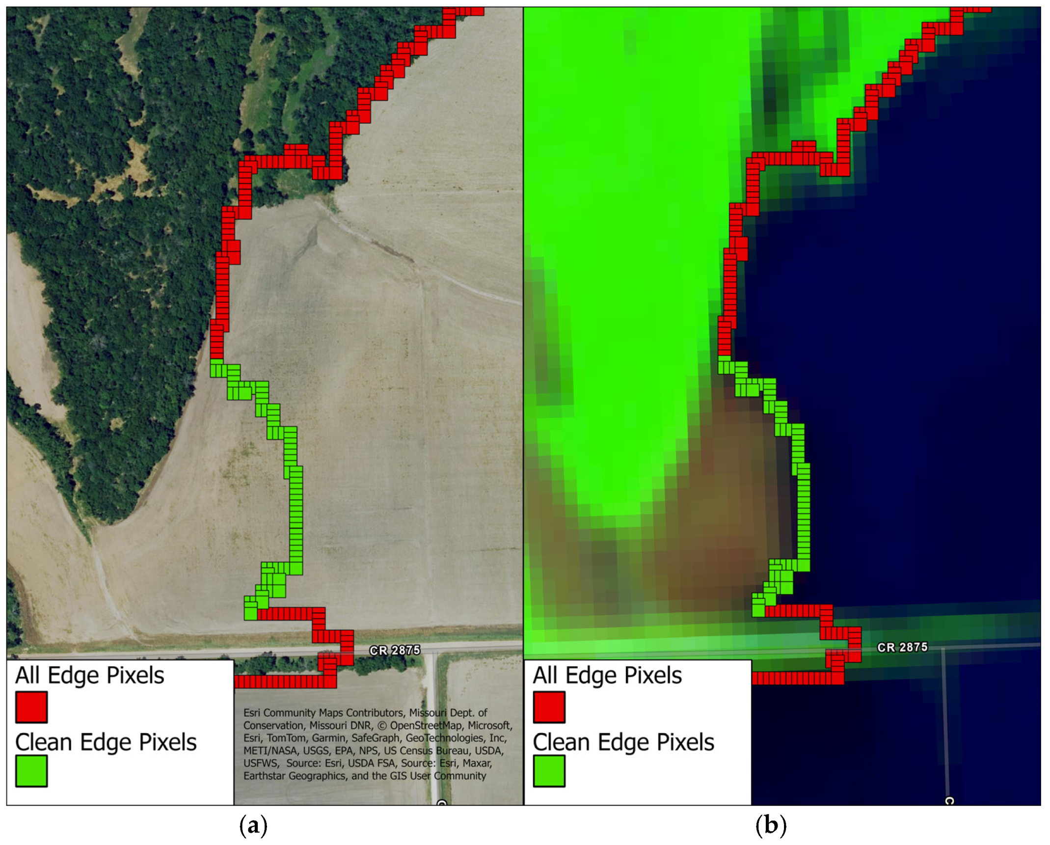
For this study, clouds were removed using the Cloud Score+ dataset with a threshold of 0.3. Land cover, including permanent water bodies, trees, urban areas, wetlands, and crops from the NLCD 2019 dataset, was used as exclusion masks. A normalized difference vegetation index (NDVI) mask was also applied to remove any potential vegetation that may have been missing in the land cover masks, and any pixels with an NDVI above 0.3 were masked out. Any water-edge pixels with a 2-pixel buffer of the masks were removed, and the rest are identified as clean flood edge pixels. A slope threshold between 2 and 20 degrees was further applied to remove clean pixels that were either too flat or too steep, which could negatively impact water depth estimation [25]. Figure 3 illustrates an example of both clean and unclean-edge pixels, with unclean-edge pixels bordering trees, while clean-edge pixels border bare ground.
This step was performed on GEE with the Clean Flood Edge Extractor web application implemented using JavaScript. The GEE app allows users to define imagery date, land cover masks, and additional parameters such as area of interest, threshold values for MNDWI, NDVI, cloud score, slope, small water body size, and buffer size. Identified clean-edge pixels are then exported from GEE.

3.3. Estimate FSP DOF Using Clean Flood Edge Pixels

Normally, the FLDPLN FIM works by obtaining FSP DOF values from gauge observations. FSP DOFs between gauges are then interpolated. An FPP is considered flooded if the DOF at an FSP, which can inundate the FPP, is higher than the DTF. In FLDSensing, clean flood edge pixels, which have a flood depth close to, ideally, zero, act as synthetic gauges to estimate the DOFs at the FSPs that can inundate those edge pixels. Those FSP DOFs are then interpolated and used to generate a flood depth map.

3.3.1. Identify FSPs and Estimate Their DOFs

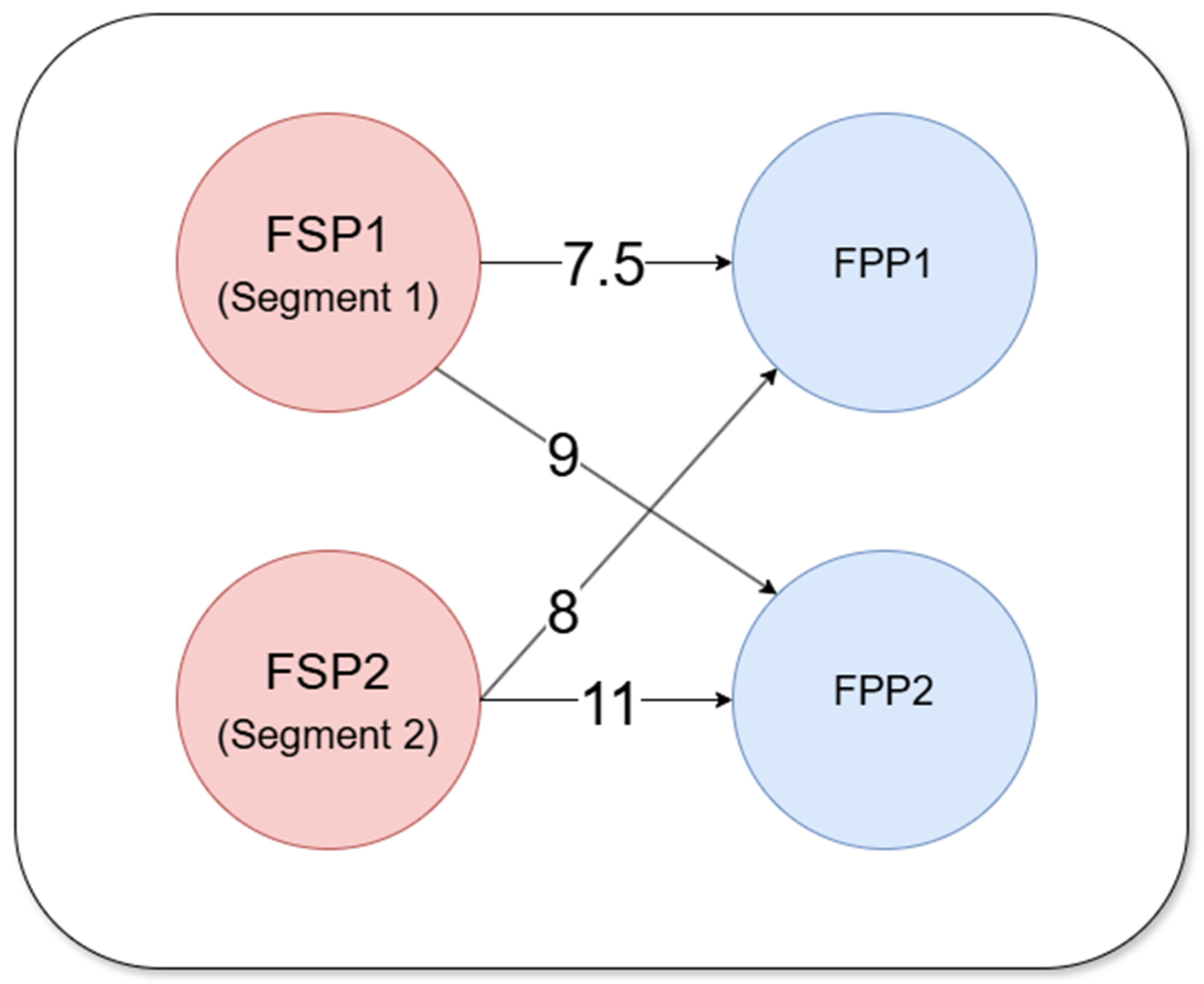
Given the many-to-many nature of the FSP-FPP flooding relationship, an edge FPP can potentially be flooded by multiple FSPs. This can lead to many DOFs depending on which FSPs are selected to flood the FPP. FLDSensing iterates through all possible DOF combinations for all edge FPPs and selects the combination that gives the least total flood depth at those FPPs [31] (pp. 48–60). In Figure 4, FSP1 and FSP2 can inundate both edge pixels FPP1 and FPP2. The DTFs for FSP1 to inundate FPP1 and FPP2 are 7.5 and 9, respectively, so the DOF at FSP1 can be 7.5 or 9. The DTFs for FSP2 to inundate FPP1 and FPP2 are 8 and 11, respectively, so the DOF at FSP2 could be 8 or 11. Table 1 shows all the possible DOF combinations at the FSPs and their resulting flood depths at the two FPPs. Case 3, with the DOFs of 9 and 8 at FSP1 and FSP2, respectively, is the best combination, as it produces the least total flood depth of 1.5 for both FPPs. As a result, the DOFs at FSP1 and FSP2 are assigned to 9 and 8, respectively. Case 1 is discarded due to the negative flood depth at FPP2. If no valid combination is found, the corresponding clean-edge pixels are excluded from further consideration.
Iterating through all possible DOF combinations might be computationally infeasible with too many DOFs. To manage this, a user input option of a maximum combination threshold (default to 100,000) was used to prevent extreme runtime. When the total number of combinations exceeds this limit, DOFs are filtered using an incremental threshold of 0.1 to reduce the amount of similar DOFs. This filtering continues with an increased threshold, if necessary, until the total number of combinations is reduced below the user input threshold.

3.3.2. Filter FSPs by Stream Order

The inclusion of all the FSPs from all streams can lead to a significant overestimation of flood extent, as floodwater may not occur in all the streams. A solution to this problem is that after the optimal FSP DOFs are obtained, those FSPs are further filtered based on their stream orders, and only the FSPs along the dominant stream order are retained. The reasoning behind this is that the imagery will represent where flooding is occurring and, in turn, will determine where clean flood edge pixels are delineated from the resulting remote sensing imagery.

3.4. Smooth DOFs and Generate Flood Inundation Map

The Savitzky–Golay filter [32], which smooths data points by fitting successive data points with a low-degree polynomial using a method of linear least squares, is applied to smooth the DOFs along the stream to reduce errors caused by erroneous edge pixels. The filter has two parameters: the window size, which determines the number of neighboring data points used, and the degree to which the polynomial is fitted. A high window size and a low polynomial degree produce a more gradual water surface elevation profile and prevent overfitting to local variations [33]. This helps to create a more consistent flood extent while minimizing over- or under-flooding. In this research, the window size is set big enough to include almost all the FSPs along a stream order and rounds down to either the nearest hundred or the nearest thousand, depending on the total number of FSPs along the stream order. For example, if there are 656 total FSPs along a stream order, the window size will be automatically set to the lowest hundred plus one (601), and if there are 1281 FSPs along a stream order, the window size will then be 1001. After the smoothing is complete, a final flood inundation depth grid is generated.

3.5. Ground Truth and Accuracy Metrics

A HEC-RAS 2D model was generated for the study area to simulate the Verdigris River flood event using USGS gauge data, and 5 m LiDAR DEM data was used to generate the FLDPLN library. The HEC-RAS 2D numerical model has been used and validated over multiple study areas worldwide for different types of floods and hydrodynamic conditions [34,35,36,37]. The modeled flood extent and depths are used as ground truth to evaluate our method for the same time when the satellite image was captured. For flood extent accuracy metrics, Critical Success Index (CSI), Probability of Detection (POD), False Alarm Ratio (FAR), and F1 Score, which are defined in Table 2, are used. CSI answers how well the forecast corresponds to the observed, POD answers what fraction of the observed was correctly forecasted, and FAR answers what fraction of the predicted did not occur [38]. The calculations of the evaluation metrics are performed using the NOAA-OWP GVAL Python package [39].
For depth accuracy assessment, percent bias (PBIAS) (4) and root mean square error (RMSE) (5) are used. PBIAS has a target score of 0, representing an unbiased depth simulation. A positive PBIAS represents a tendency of overestimation, while a negative PBIAS represents a tendency of underestimation [40]. A lower RMSE score indicates a better agreement between simulated and observed flood depth.
P B I A S = 100 i = 1 N ( S i O i ) i = 1 N ( O i )
R M S E = 1 n i = 1 N ( S i O i ) 2
where N is the number of raster cells where both maps indicate inundation, S is FLDSensing depth, and O is HEC-RAS depth.

4. Results

4.1. HEC-RAS 2D Inundation Map

Flood dynamics along the Verdigris River between USGS gauge 07170500 and USGS gauge 07170990 were simulated using a two-dimensional HEC-RAS model (version 6.5) in 2D configuration (HR2D). The governing equations are based on the shallow-water equations and solved through the Eulerian–Lagrangian Method (SWE–ELM). The modeled river reach extends approximately 60 km in length, covering a total flood domain of 190 km2. A 48 h warm-up period was included to stabilize the initial hydraulic conditions of the model. The turbulence model was set to conservative, with longitudinal and transverse mixing coefficients assigned to default values, as no field velocity measurements were available for calibration. A fixed computational time step of 30 s was adopted, with adaptive adjustment allowed between 15 and 60 s depending on the Courant number to maintain numerical stability. The HR2D model was defined and built using the System International (metric system) units. Results generated are exported to the United States unit systems.
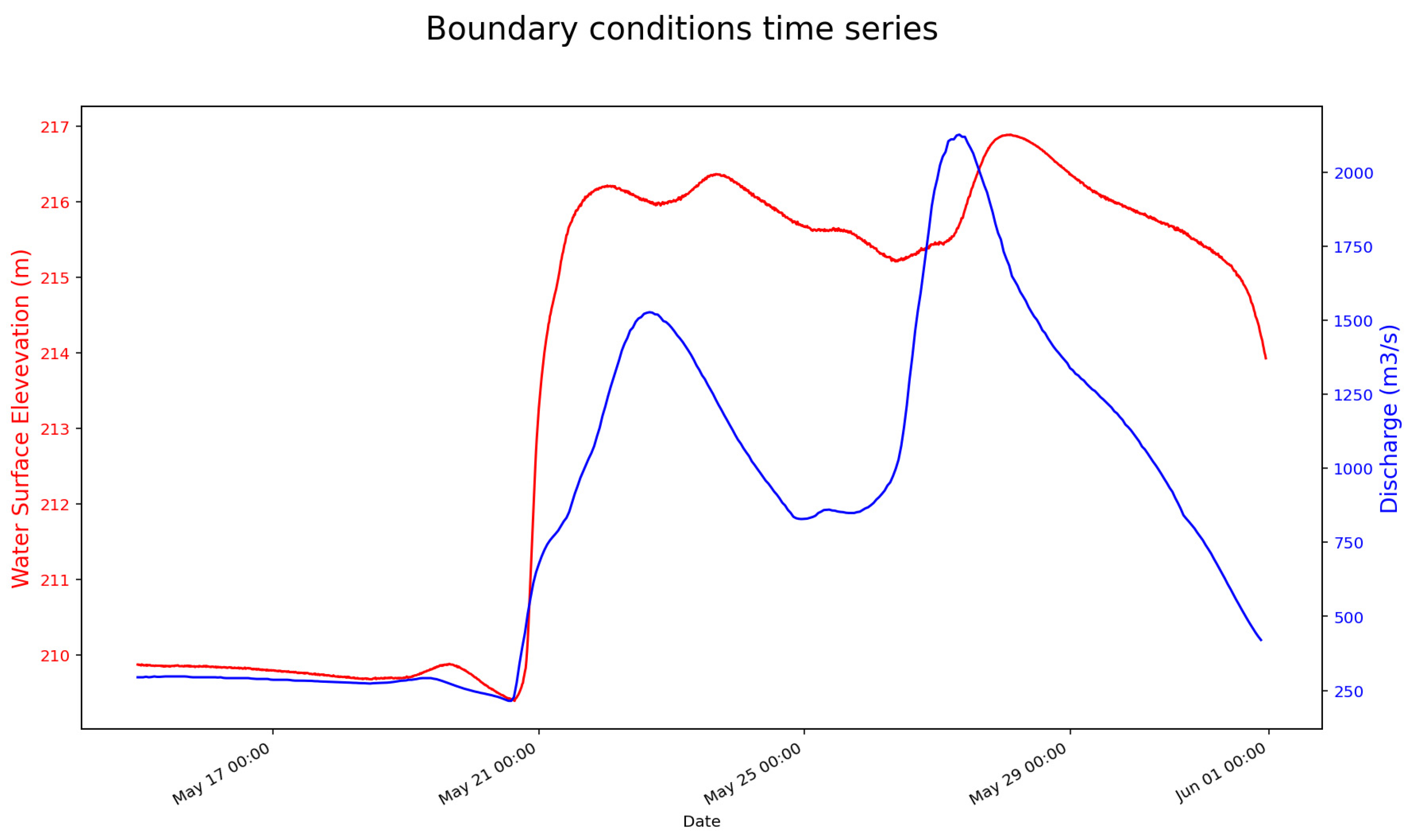
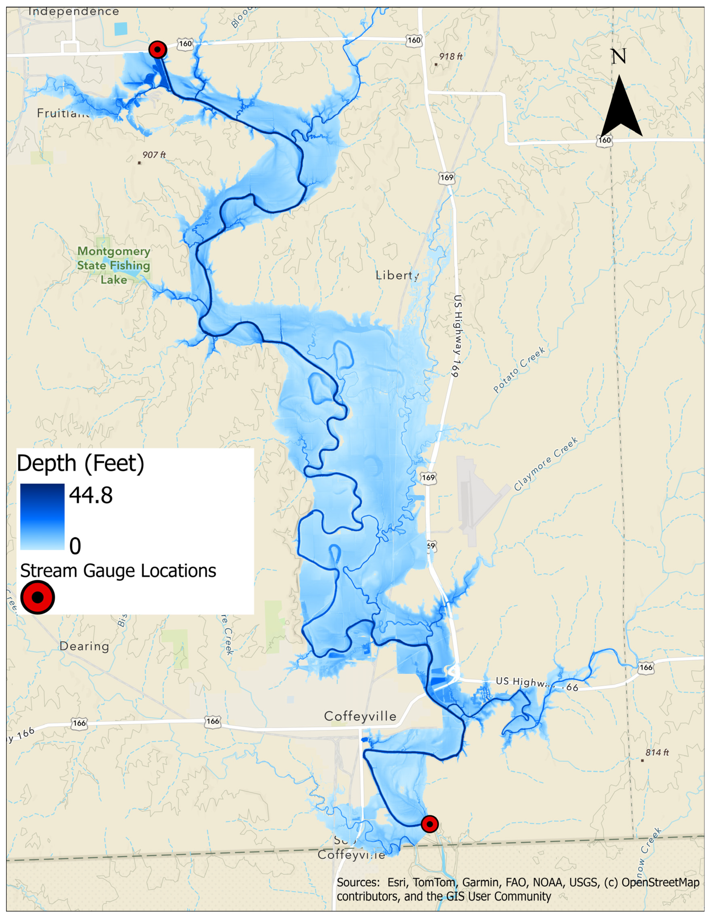
The model domain was discretized into 40,982 computational cells with an adaptive mesh, consisting of a base resolution of 75 × 75 m and refinement to 12 × 12 m in areas requiring detailed representation of hydraulic features. This flexible mesh adjusts cell sizes according to breaklines, ensuring that the main Verdigris River channel is represented by at least four cells across its width. Breaklines were introduced to preserve topographic controls along levees, embankments, and channel centerlines (Figure 5). Terrain data used was derived from the 5 m LiDAR DEM. The DEM was hydro-conditioned to ensure channel connectivity and account for bridges and other man-made structures. Boundary conditions were defined using hourly discharge at the USGS gauge 07170500 (upstream) and water surface elevation at the USGS gauge 07170990 (downstream) (Figure 6), with data retrieved from the USGS online web service. The total computational time window modeled was between 14 and 30 May 2019.
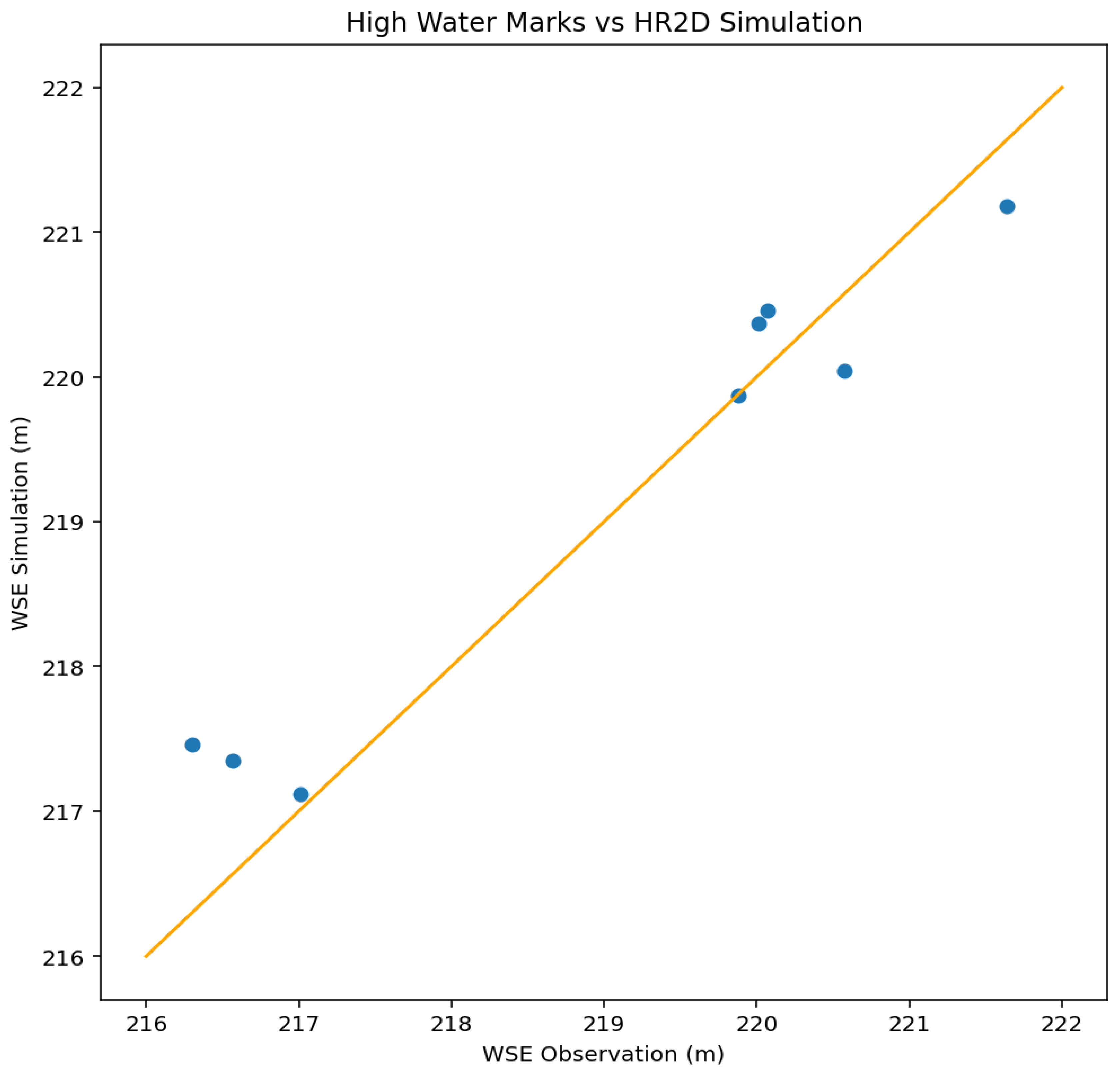
Spatially distributed Manning’s roughness coefficients were derived from the 2019 National Land Cover Database (NLCD), where land cover classes were grouped into five categories for simplicity: (i) developed/urban areas, (ii) forests/wetlands, (iii) open water, (iv) barren land, and (v) agricultural land. Roughness values were assigned following recommended ranges in previous studies [41,42,43,44]. Calibration was conducted by running ten simulations varying Manning’s coefficients (Table 3) within these literature ranges and selecting the combination that minimized the RMSE against observed USGS high-water marks. Due to the lack of continuous water surface elevation time series in the study domain, temporal model performance could not be directly evaluated, relying only on high-water marks data. The maximum water surface elevations from the model were compared with high-water marks collected by the USGS Flood Event Viewer (https://stn.wim.usgs.gov/FEV/ (accessed on 2 October 2025). The comparison yielded a root mean square error of 0.58 m (1.90 ft), consistent with previous riverine flood applications (Figure 7). Flood extents and depths were further compared with Sentinel-2 imagery acquired at local noon of 27 May 2019 (Figure 8), showing good agreement with observed inundation patterns. Results of hourly WSE, depths, and hydraulic profile can be generated using the RAS Mapper tool included in HEC-RAS software. These results serve as a benchmark to compare the performance of the method proposed in this study.
Simulations were executed on a Windows workstation equipped with an Intel Core i5 CPU (3.40 GHz), 64 GB RAM, and using 14 solver cores. The average runtime per 2D simulation was approximately 40 min. We acknowledge that parallelization of HEC-RAS 2D is not supported under Windows, as simulations are usually conducted in a serial configuration, which made extensive calibration scenarios computationally prohibitive. Future work could explore Linux-based implementations and HPC environments to more comprehensively assess parameter and mesh resolution uncertainty for this study area [36].

4.2. Remote Sensing-Based FIM

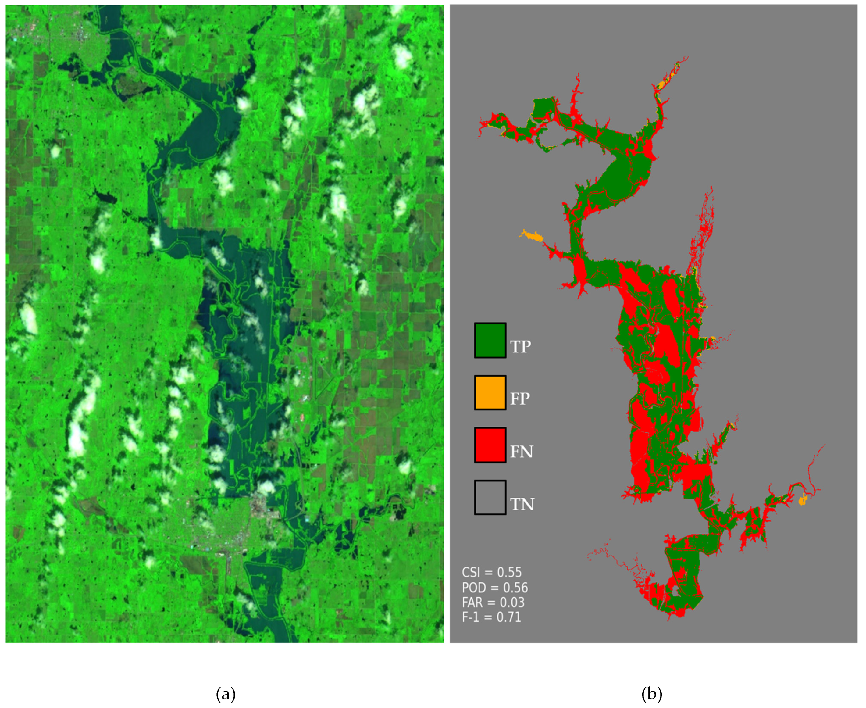
The Sentinel-2 remote sensing only FIM (Figure 9) was generated using MNDWI with an optimal threshold of 0.09. Clouds were removed using the Cloud Score+ dataset with a CS band threshold of 0.3. Small waterbodies less than three hectares were removed to reduce the influence of small ponds or pluvial flooding on the metrics.
Figure 9b shows the poor performance of using a purely remote sensing-based FIM with CSI, POD, FAR, and F1 having values of 0.55, 0.56, 0.03, and 0.71, respectively. This is caused by clouds and vegetation canopy, which obscure the floodwater from the Sentinel-2’s optical sensor and significantly underestimate the flood inundation extent. In addition, remote sensing FIM cannot estimate flood depth, which makes the map less valuable for emergency responders and decision-makers.

4.3. FLDSensing FIM

Using the cloud, 2019 NLCD and NDVI (>0.3) as a combined mask, and a slope between 2 and 20 degrees, a total of 144 clean water-edge pixels were identified from the Sentinel-2 imagery. The flood occurred mainly along the mainstem of the Verdigris River (one of the six stream orders in the study area), which has the largest number of FSPs (46) that inundate those clean-edge pixels. After applying the vertical interpolation with the 46 FSP DOFs, a total of 14,452 FSP DOFs along the mainstem are obtained. The Savitzky–Golay filter was further applied with a polynomial degree of 2 and a window size of 14,001.
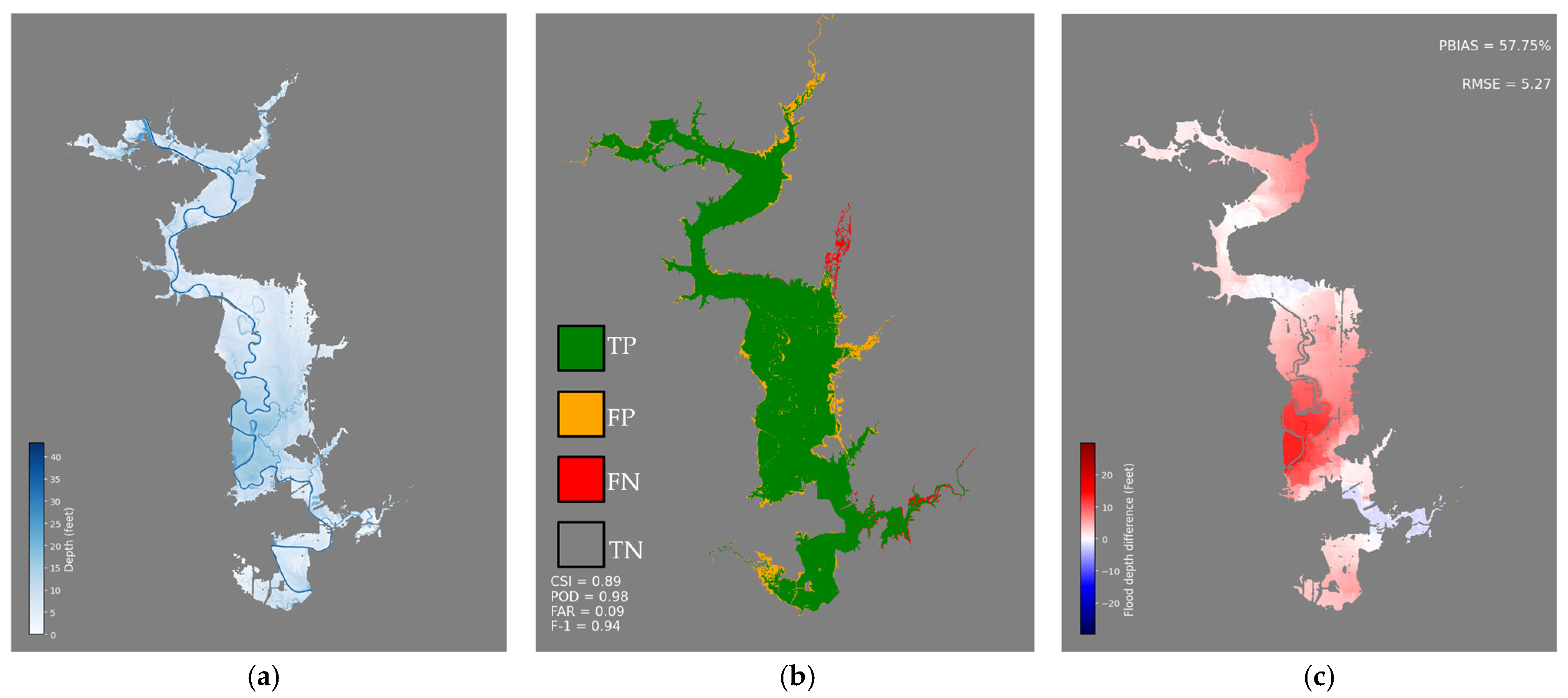
The result of FLDSensing maps and metrics is shown in Figure 10 and Table 4, with CSI, POD, FAR, and F1 having the values of 0.89, 0.98, 0.09, and 0.94, respectively. The performance is greatly improved compared to the remote sensing map, with a double-digit increase in the metrics showcasing FLDSensing’s ability to accurately estimate flood extent and depth. Overall, there is an overestimation of the extent surrounding the flooded area and some underestimation in the south of the study area, and some underestimation in the northeast, as well as some underestimation in the center north of the study area. The amount of false positive pixels equals 299,201, and the number of false negatives equals 67,149. The depth map, with a PBIAS of 57.75%, shows a general overestimation, especially in the middle region of the flooded area. With an RMSE of 5.27 feet, it represents an improvement over the innate inability of remote sensing-based FIM to directly provide a flood depth map.

4.4. Comparison with the FLEXTH and FwDET Methods

A comparison with the FLEXTH (commit: 87059438) and FwDET 2.1 (commit: ec4e1cd) methods was also conducted to evaluate FLDSensing’s performance compared with other popular hybrid approaches. Both methods use the most recent version retrieved from their respective GitHub repositories as of 10 April 2025. Both are compared with the HEC-RAS 2D benchmark maps to evaluate their performance in terms of extent and depth estimation.

4.4.1. FwDET

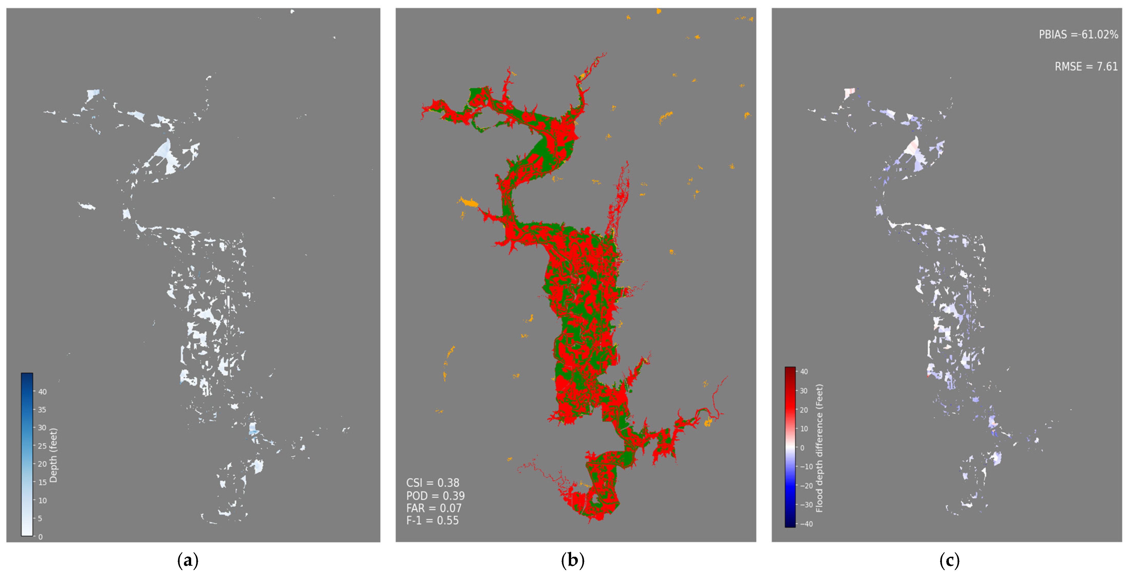
The same 5 m LiDAR DEM as in FLDSensing and the Sentinel-2-derived flood extent map (with the Cloud Score+ threshold raised from 0.3 to 0.5 to sharpen boundary cells adjacent to clouds) were used as inputs for FwDET 2.1. The model was then run using its default settings of three smoothing iterations on the boundary-cell depths and a one-degree slope threshold. The results are shown in Figure 11 and Table 5. The extent metrics for FwDET are low, even compared to those of remote sensing-only FIM. It is worth noting that FwDET does not generate flood extent but rather estimates flood depth with an existing extent map. The significant reduction (i.e., the presence of many “holes”) in the resulting flood extent is due to incorrect boundary cells’ water surface elevation estimation using DEM, where the boundary cells are not clean water-edge pixels. Negative depth values resulting from incorrect boundary cells are automatically filtered, effectively shrinking the flood extent in the output depth map.

4.4.2. FLEXTH

FLEXTH has two required inputs, a binary flood extent map and a DEM, and two optional inputs, an exclusion mask and a reference permanent water mask. The flood extent map generated without the Cloud Score+ masking and the 5 m LiDAR DEM are used as the required inputs to run FLEXTH. Cloud Score+ was not used, as testing found that using an extreme cloud mask hindered results, as FLEXTH relies on as complete an input flood inundation map as possible. FLEXTH would perform best if used alongside SAR imagery to see inundation underneath cloud cover. The exclusion mask is an automatically generated product from the GFM that identifies areas (such as flat areas, dense vegetation, and urban areas) that could be potentially inundated. Since the GFM only uses Sentinel-1 imagery, an exclusion mask is not available for the Sentinel-2 image (27 May 2019) used for FLDSensing. Instead, the exclusion mask captured five days earlier (22 May 2019) by Sentinel-1 was used. This time difference should not have much impact on the exclusion mask, which should not change significantly in five days. The reference water mask identifies pixels of seasonal and permanent water bodies to limit floodwater propagation and is also generated from the Sentinel-1 imagery on 22 May 2019. With the above inputs, FLEXTH was run using all default settings except for the parameter that allows inundation to propagate into areas not covered by the exclusion mask. This parameter was enabled to allow more areas to be inundated to improve the model’s performance.
The results from FLEXTH are shown in Figure 12 and Table 5. While FLEXTH is much better than remote sensing-based FIM, FLDSensing still generally outperforms FLEXTH in terms of extent, with CSI improving from 0.81 to 0.89, POD from 0.90 to 0.98, FAR from 0.11 to 0.09, and F1 from 0.89 to 0.94. Flood depth from FLEXTH tends to be underestimated, especially in the middle of the flooded domain, resulting in a PBIAS of -29.98% and an RMSE of 3.38 feet, which is a better estimation than FLDSensing.
FLEXTH tends to underestimate flood extent due to its limitations in a more simplified approach to flood propagation. While the latest update to FLEXTH allows floodwater to propagate into areas beyond the exclusion mask and remedies the flood extent underestimation, it is still not as robust as the FLDSensing method, which relies on the FSP-FPP-DTF inundation relationships derived by the FLDPLN model. Pluvial flooding also has a notable influence on FLEXTH results, as the algorithm permits any pixel to inundate a neighboring pixel provided it satisfies four key criteria. The pixel must belong to the exclusion mask; the neighboring pixel must have a DEM elevation lower than the current water level; the propagated water level in the neighboring pixel must remain lower than that of the source pixel; and the neighboring pixel must not already be inundated. In contrast to FLDSensing’s approach of using FSPs attached to a stream order to spread floodwater, rule number one of FLEXTH propagation criteria can be ignored if the parameter mentioned previously is used, which is used in this study. FLEXTH also does not use as rigorous a clean water-edge pixel extraction process as FLDSensing does, which runs the risk of drastic over-flooding or under-flooding if they are misidentified or not automatically removed from the GFM exclusion mask.

5. Discussion

5.1. The Tributary Problem

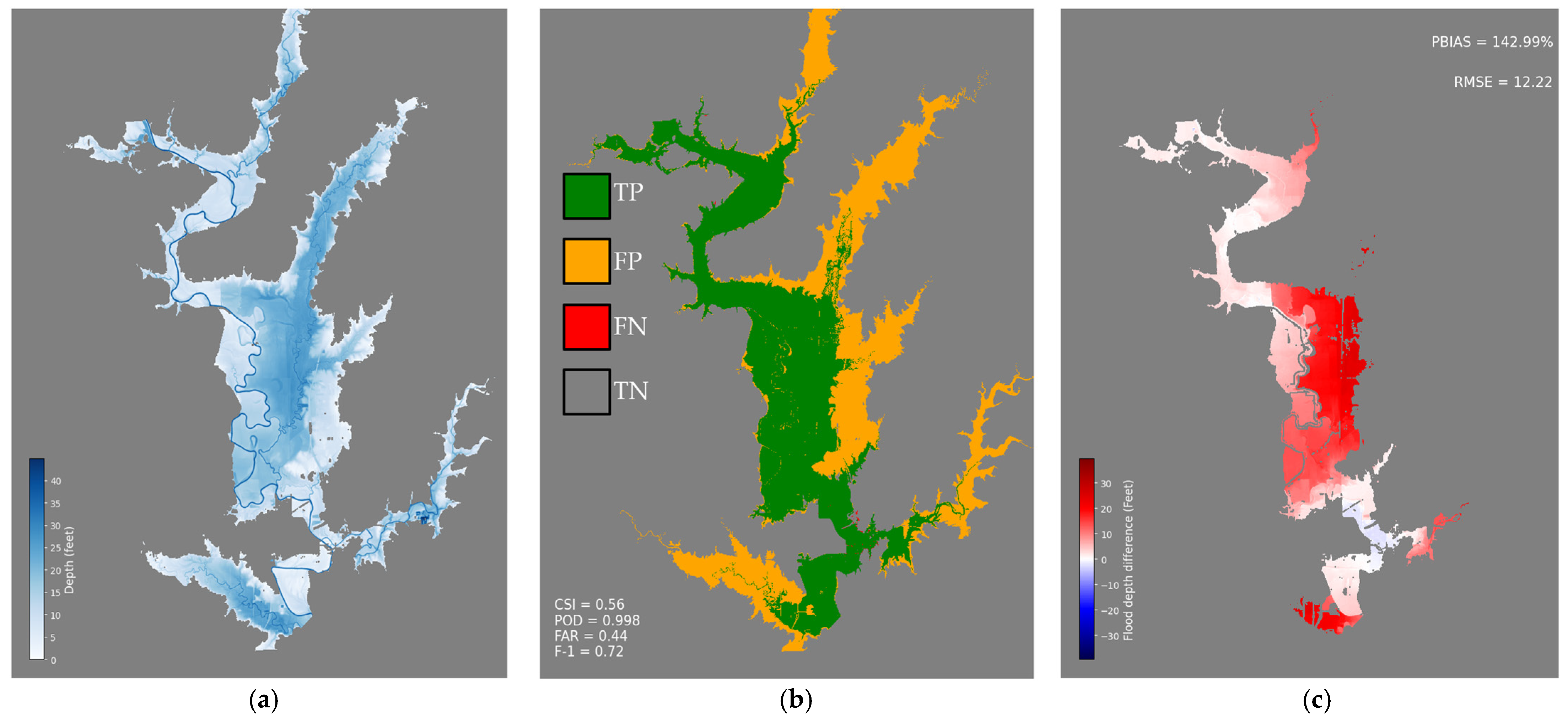
A clean water-edge pixel (i.e., an FPP) can be flooded in FLDPLN by FSPs from the mainstem, tributaries, or both at the same time during flood events spanning a large area. The inclusion of all the FSPs for the Verdigris flood event can result in the overestimation of flood extent (Figure 13), with CSI changing from 0.89 to 0.56, POD from 0.98 to 0.998, FAR from 0.09 to 0.44, F1 from 0.94 to 0.72, PBIAS from 57.75% to 142.99%, and RMSE from 5.27 feet to 12.22 feet. This overestimation of both extent and depth highlights the need to identify where floodwater comes from when using FLDSensing.
Currently, we use the FSPs from all the streams, regardless of where the floodwater comes from, and decide their DOFs that give the least total flood depth at the clean-edge pixels. This could result in a clean-edge pixel being assigned to tributary FSPs when there is no floodwater from the tributary but instead from the mainstem, or vice versa. To reduce this problem, we implemented a process where we select the stream order that has the dominant amount of FSPs, with the reasoning being that imagery will represent where inundation is from, whether that be from a tributary or the mainstem. A limitation of this approach is that if a flood does occur simultaneously along both the mainstem and a tributary, then the inundation might be underestimated.
While the FLDSensing method can be run on single or multiple stream orders, it currently cannot automatically detect which stream order(s) have floodwater. However, our current implementation, as described above and in Section 3.3.2, automatically detects the dominant stream order and assumes that it is the only stream that causes flood inundation. If the user wants to use different or multiple stream orders, for example, based on visual image examination, the change can be made within the Jupyter Notebook (commit: ce3036f).

5.2. Impacts of the Savitzky–Golay Filter

The FLDSensing results without using the Savitzky–Golay data smoothing technique are shown in Figure 14. When compared to the result using the Savitzky–Golay filter, the performance metrics show a decrease, with CSI falling from 0.89 to 0.75, POD staying the same, FAR going from 0.09 to 0.24, and F1 going from 0.94 to 0.86. Depth PBIAS also goes from 57.75% to 135.69%, and RMSE goes from 5.27 feet to 10.06 feet. The original FLDSensing elevation is choppy with drastic variations as it goes along the mainstem when compared to the water surface elevation with that of the HEC-RAS model. These fluctuations are removed or lessened by utilizing the Savitzky–Golay filter to improve the performance of the FLDSensing method.
We performed a sensitivity analysis by using different window sizes (Table 6). We found that smaller window sizes lead to overflooding caused by stage spikes along the stream. As shown in the table, the method performed the best with a window size (14,001) covering the entire stream pixels, which is the size used in this study.

5.3. Model Parameters, Uncertainty, and Best Practices

Detecting clean-edge pixels is one of the most important factors in FLDSensing, as incorrect edge pixels could result in an incorrect estimation of FSP DOFs. In most cases, users should be very conservative when delineating clean-edge pixels, as FLDSensing only needs a small set of high-quality clean-edge pixels to produce an output. As such, we applied a conservative set of thresholds focused on maximizing the quality of flood edge pixels. For cloud masking, we used a Cloud Score+ threshold of 0.3, though this parameter should be adjusted based on the image used. Vegetation was excluded with an NDVI threshold (0.3 as the default), chosen to ensure that even stressed or partially canopied vegetation was removed, preventing edge pixels along flood–vegetation boundaries. Floodwater was segmented using an Otsu-derived MNDWI threshold of 0.09, selected specifically for the image used in this study but with the expectation that it is automatically calculated for other imagery. To avoid edge pixels from non-flood waterbodies, we also applied a 3 ha minimum waterbody mask, which removes small ponds, ditches, and artificial reservoirs, as well as localized pluvial flooding features. A two-pixel buffer was also applied collectively to all the masks created using the above parameters to increase rigor in clean-edge pixel delineation. Collectively, these parameters prioritize quality over quantity by discarding potentially problematic water-edge pixels.
For this study, using the NLCD 2019 landcover dataset, a combined cloud and land cover mask, including permanent water bodies, trees, urban areas, wetlands, and crops, helped identify clean water-edge pixels. Land cover types should always be examined by the user to determine the most appropriate types depending on the study area. The user should also decide on an appropriate NDVI threshold depending on the time of year the remote sensing image was taken.
Cloud masking also plays an important role in delineating clean-edge pixels, as clouds, like tall vegetation, could also have floodwater underneath. However, if the remote sensing image has almost no clouds, the user can be more aggressive with cloud masking to achieve more accurate, clean-edge pixels. In images where cloud cover is heavy, aggressive cloud masking could lead to too few clean water-edge pixels, and the user, in this scenario, should reduce the Cloud Score+ threshold.
The FSP DOF combination threshold is not intended to be a fixed number but instead a parameter that can change depending on the number of selected FSPs and runtime. We tested five thresholds ranging from 10,000 to 1 million, which showed little improvement in the performance metrics except in the runtime. The 100,000-threshold took around 40 s to complete, while the one-million-threshold took about 8 min, but without much benefit on a standard consumer-grade laptop. This drastic increase in runtime shows the need for the user to set a combination threshold to prevent excessive runtime. For our study, we found that the 100,000-threshold worked well enough and was chosen as the default unless the user wants to change it.

6. Conclusions

By identifying clean floodwater-edge pixels from satellite imagery and combining them with the FLDPLN library to estimate stream stage, the proposed FLDSensing method was able to improve flood extent and depth mapping when compared with remote sensing only FIM. When applied to the 2019 flood event along the Verdigris River, our method achieved impressive metrics with CSI, POD, and F1 scores exceeding or close to 0.9 while keeping FAR low at around 0.09 when compared to the HEC-RAS 2D benchmark, with a depth PBIAS of 57.75% and a depth RMSE of 5.27 feet.
FLDSensing showed substantial improvement over FwDET in both flood extent and depth estimation, with FwDET underestimating depth through the entire flood area, primarily due to incorrect identification of boundary cells in the model. Compared to FLEXTH, FLDSensing flood extent estimation outperforms FLEXTH while having similar metrics in depth estimation, with FLEXTH leaning towards underestimation instead of FLDSensing’s overestimation. FLEXTH’s underestimation in flood extent is primarily due to a more simplified method of flood propagation when compared to the FLDPLN model used in the FLDSensing method.
FLDSensing can be further improved in clean-edge detection from satellite imagery and selecting appropriate stream pixels for stage estimation. Clean-edge pixel delineation could benefit from further examination of the semi-automated method implemented on the GEE, which could lead to erroneous clean-edge pixels and subsequent incorrect stream stage estimation. FLDSensing currently cannot automatically detect where floodwater originates; future work should include a method to detect which stream order is experiencing a flood event. Future work could also include expanding data sources beyond Sentinel-2 to include Landsat, Sentinel-1, or alternative platforms such as drones, traffic cameras, or field observations.

Author Contributions

Conceptualization X.L., S.C., J.E., F.J.G. and S.K.D.; data curation J.K. and D.A.W.; methodology J.E., S.K.D., F.J.G., X.L. and S.C.; project administration X.L. and S.C.; software J.E., S.K.D., F.J.G., X.L. and J.K.; supervision X.L., S.C., H.M. and V.L.; validation F.J.G., S.K.D. and J.E.; visualization J.E., F.J.G. and S.K.D.; writing—original draft J.E.; writing—review and editing X.L., S.K.D. and F.J.G.; funding acquisition., X.L., J.K. and S.C. All authors have read and agreed to the published version of the manuscript.

Funding

Funding for this project was supported by the Cooperative Institute for Research to Operations in Hydrology (CIROH) through its Summer Institute and Visiting Scholar programs, with funding under award NA22NWS4320003 from the NOAA Cooperative Institute Program, and by the Kansas Water Office.

Data Availability Statement

The links to the GEE app, FLDSensing GitHub, and the FLDPLN library are listed below. The HEC-RAS 2D model is available upon request, and all the data to build the model is available online. GEE App: https://code.earthengine.google.com/f3c44ca8a4aa6ce9d45c122ddb0d19e1 (accessed on 25 September 2025); FLDSensing GitHub: https://github.com/NWC-CUAHSI-Summer-Institute/FLDSensing (accessed on 25 September 2025); FLDPLN library: https://kbs-karsfl-pc01.home.ku.edu/download/verdigris_library.zip (accessed on 25 September 2025).

Conflicts of Interest

The authors declare no conflicts of interest.

Abbreviations

The following abbreviations are used in this manuscript:
FSPFlood Source Pixel
FPPFloodplain Pixel
DTFDepth to Flood
DOFDepth of Flow
DEMDigital Elevation Model
FIMFlood Inundation Mapping
PODProbability of Detection
FARFalse Alarm Ratio
CSICritical Success Index
HANDHeight Above Nearest Drainage
GFMGlobal Flood Monitoring product
AWEIAutomated Water Extraction Index
NDWINormalized Difference Water Index
MNDWIModified Normalized Difference Water Index
GEEGoogle Earth Engine
PBIASPercent Bias
RMSERoot Mean Square Error
HR2DHEC-RAS 2D
WSEWater Surface Elevation
SARSynthetic Aperture Radar
GFMGlobal Flood Monitoring
GloFASGlobal Flood Awareness System

References

  1. Guha-Sapir, D.; Hoyois, P.; Wallemacq, P.; Below, R. Annual Disaster Statistical Review 2016. Available online: https://www.emdat.be/sites/default/files/adsr_2016.pdf (accessed on 10 August 2024).
  2. Nobre, A.D.; Cuartas, L.A.; Hodnett, M.; Rennó, C.D.; Rodrigues, G.; Silveira, A.; Waterloo, M.; Saleska, S. Height Above the Nearest Drainage—A hydrologically relevant new terrain model. J. Hydrol. 2011, 404, 13–29. [Google Scholar] [CrossRef]
  3. Kastens, J.H. Some New Developments on Two Separate Topics: Statistical Cross Validation and Floodplain Mapping. 2008. Available online: https://kuscholarworks.ku.edu/handle/1808/5354 (accessed on 22 April 2024).
  4. Shustikova, I.; Domeneghetti, A.; Neal, J.C.; Bates, P.; Castellarin, A. Comparing 2D capabilities of HEC-RAS and LISFLOOD-FP on complex topography. Hydrol. Sci. J. 2019, 64, 1769–1782. [Google Scholar] [CrossRef]
  5. Aristizabal, F.; Salas, F.; Petrochenkov, G.; Grout, T.; Avant, B.; Bates, B.; Spies, R.; Chadwick, N.; Wills, Z.; Judge, J. Extending Height Above Nearest Drainage to Model Multiple Fluvial Sources in Flood Inundation Mapping Applications for the U.S. National Water Model. Water Resour. Res. 2023, 59, e2022WR032039. [Google Scholar] [CrossRef]
  6. Salmoral, G.; Casado, M.R.; Muthusamy, M.; Butler, D.; Menon, P.P.; Leinster, P. Guidelines for the Use of Unmanned Aerial Systems in Flood Emergency Response. Water 2020, 12, 521. [Google Scholar] [CrossRef]
  7. Mohney, D.; Terabytes from Space: Satellite Imaging is Filling Data Centers. Data Center Frontier. Available online: https://www.datacenterfrontier.com/internet-of-things/article/11429032/terabytes-from-space-satellite-imaging-is-filling-data-centers (accessed on 25 March 2025).
  8. Tarpanelli, A.; Mondini, A.C.; Camici, S. Effectiveness of Sentinel-1 and Sentinel-2 for Flood Detection Assessment in Europe. Nat. Hazards Earth Syst. Sci. 2022, 22, 2473–2489. [Google Scholar] [CrossRef]
  9. Mcfeeters, S.K. The use of the Normalized Difference Water Index (NDWI) in the delineation of open water features. Int. J. Remote Sens. 1996, 17, 1425–1432. [Google Scholar] [CrossRef]
  10. Xu, H. Modification of normalised difference water index (NDWI) to enhance open water features in remotely sensed imagery. Int. J. Remote Sens. 2006, 27, 3025–3033. [Google Scholar] [CrossRef]
  11. Feyisa, G.L.; Meilby, H.; Fensholt, R.; Proud, S.R. Automated Water Extraction Index: A new technique for surface water mapping using Landsat imagery. Remote Sens. Environ. 2014, 140, 23–35. [Google Scholar] [CrossRef]
  12. Dartmouth Flood Observatory. Available online: https://floodobservatory.colorado.edu/Archives/ (accessed on 28 April 2025).
  13. Hamidi, E.; Peter, B.G.; Muñoz, D.F.; Moftakhari, H.; Moradkhani, H. Fast Flood Extent Monitoring with SAR Change Detection Using Google Earth Engine. IEEE Trans. Geosci. Remote Sens. 2023, 61, 1–19. [Google Scholar] [CrossRef]
  14. Roth, F.; Tupas, M.E.; Navacchi, C.; Zhao, J.; Wagner, W.; Bauer-Marschallinger, B. Evaluating the robustness of Bayesian flood mapping with Sentinel-1 data: A multi-event validation study. Sci. Remote Sens. 2025, 11, 100210. [Google Scholar] [CrossRef]
  15. Clement, M.A.; Kilsby, C.G.; Moore, P. Multi-temporal synthetic aperture radar flood mapping using change detection. J. Flood Risk Manag. 2018, 11, 152–168. [Google Scholar] [CrossRef]
  16. Do, S.K.; Du, T.L.T.; Lee, H.; Chang, C.; Bui, D.D.; Nguyen, N.T.; Markert, K.N.; Strömqvist, J.; Towashiraporn, P.; Darby, S.E.; et al. Assessing Impacts of Hydropower Development on Downstream Inundation Using a Hybrid Modeling Framework Integrating Satellite Data-Driven and Process-Based Models. Water Resour. Res. 2025, 61, e2024WR037528. [Google Scholar] [CrossRef]
  17. Jo, M.-J.; Osmanoglu, B.; Zhang, B.; Wdowinski, S. Flood Extent Mapping Using Dual-Polarimetric Sentinel-1 Synthetic Aperture Radar Imagery. Int. Arch. Photogramm. Remote Sens. Spat. Inf. Sci. 2018; XLII-3, 711–713. [Google Scholar] [CrossRef]
  18. Amitrano, D.; Di Martino, G.; Di Simone, A.; Imperatore, P. Flood Detection with SAR: A Review of Techniques and Datasets. Remote Sens. 2024, 16, 656. [Google Scholar] [CrossRef]
  19. Klemas, V. Remote Sensing of Floods and Flood-Prone Areas: An Overview. J. Coast. Res. 2015, 31, 1005–1013. [Google Scholar] [CrossRef]
  20. Betterle, A.; Salamon, P. Water depth estimate and flood extent enhancement for satellite-based inundation maps. Nat. Hazards Earth Syst. Sci. 2024, 24, 2817–2836. [Google Scholar] [CrossRef]
  21. Cohen, S.; Brakenridge, G.R.; Kettner, A.; Bates, B.; Nelson, J.; McDonald, R.; Huang, Y.-F.; Munasinghe, D.; Zhang, J. Estimating Floodwater Depths from Flood Inundation Maps and Topography. JAWRA J. Am. Water Resour. Assoc. 2018, 54, 847–858. [Google Scholar] [CrossRef]
  22. Cohen, S.; Raney, A.; Munasinghe, D.; Loftis, J.D.; Molthan, A.; Bell, J.; Rogers, L.; Galantowicz, J.; Brakenridge, G.R.; Kettner, A.J.; et al. The Floodwater Depth Estimation Tool (FwDET v2.0) for improved remote sensing analysis of coastal flooding. Nat. Hazards Earth Syst. Sci. 2019, 19, 2053–2065. [Google Scholar] [CrossRef]
  23. Cohen, S.; Peter, B.G.; Haag, A.; Munasinghe, D.; Moragoda, N.; Narayanan, A.; May, S. Sensitivity of Remote Sensing Floodwater Depth Calculation to Boundary Filtering and Digital Elevation Model Selections. Remote Sens. 2022, 14, 5313. [Google Scholar] [CrossRef]
  24. Aristizabal, F.; Judge, J. Mapping Fluvial Inundation Extents with Graph Signal Filtering of River Depths Determined from Unsupervised Clustering of Synthetic Aperture Radar Imagery. In Proceedings of the 2021 IEEE International Geoscience and Remote Sensing Symposium IGARSS, Brussels, Belgium, 11–16 July 2021; pp. 6124–6127. [Google Scholar] [CrossRef]
  25. Dobbs, K.E. Toward Rapid Flood Mapping Using Modeled Inundation Libraries. 2017. Available online: https://kuscholarworks.ku.edu/handle/1808/26323 (accessed on 27 February 2024).
  26. Yang, X.; Zhao, S.; Qin, X.; Zhao, N.; Liang, L. Mapping of Urban Surface Water Bodies from Sentinel-2 MSI Imagery at 10 m Resolution via NDWI-Based Image Sharpening. Remote Sens. 2017, 9, 596. [Google Scholar] [CrossRef]
  27. Pasquarella, V.J.; Brown, C.F.; Czerwinski, W.; Rucklidge, W.J. Comprehensive quality assessment of optical satellite imagery using weakly supervised video learning. In Proceedings of the 2023 IEEE/CVF Conference on Computer Vision and Pattern Recognition Workshops (CVPRW), Vancouver, BC, Canada, 17–24 June 2023; pp. 2125–2135. [Google Scholar] [CrossRef]
  28. Homer, C.G.; Fry, J.A.; Barnes, C.A. The National Land Cover Database; Report 2012–3020; Earth Resources Observation and Science (EROS) Center: Reston, VA, USA, 2012. [Google Scholar] [CrossRef]
  29. Salamon, P.; Mctlormick, N.; Reimer, C.; Clarke, T.; Bauer-Marschallinger, B.; Wagner, W.; Martinis, S.; Chow, C.; Bohnke, C.; Matgen, P.; et al. The New, Systematic Global Flood Monitoring Product of the Copernicus Emergency Management Service. In Proceedings of the 2021 IEEE International Geoscience and Remote Sensing Symposium IGARSS, Brussels, Belgium, 11–16 July 2021; pp. 1053–1056. [Google Scholar] [CrossRef]
  30. Otsu, N. A Threshold Selection Method from Gray-Level Histograms. IEEE Trans. Syst. Man Cybern. 1979, 9, 62–66. [Google Scholar] [CrossRef]
  31. Larco, K.; Mahmoudi, S. National Water Center Innovators Program Summer Institute Report 2024. 2024. Available online: https://www.cuahsi.org/uploads/pages/doc/202407_Summer_Institute_Final_Report_v2.0.pdf (accessed on 5 April 2025).
  32. Savitzky, A.; Golay, M.J.E. Smoothing and Differentiation of Data by Simplified Least Squares Procedures. Anal. Chem. 1964, 36, 1627–1639. [Google Scholar] [CrossRef]
  33. Vivó-Truyols, G.; Schoenmakers, P.J. Automatic Selection of Optimal Savitzky−Golay Smoothing. Anal. Chem. 2006, 78, 4598–4608. [Google Scholar] [CrossRef] [PubMed]
  34. Gomez, F.J.; Jafarzadegan, K.; Moftakhari, H.; Moradkhani, H. Probabilistic flood inundation mapping through copula Bayesian multi-modeling of precipitation products. Nat. Hazards Earth Syst. Sci. 2024, 24, 2647–2665. [Google Scholar] [CrossRef]
  35. Zeiger, S.J.; Hubbart, J.A. Measuring and modeling event-based environmental flows: An assessment of HEC-RAS 2D rain-on-grid simulations. J. Environ. Manag. 2021, 285, 112125. [Google Scholar] [CrossRef]
  36. Alipour, A.; Jafarzadegan, K.; Moradkhani, H. Global sensitivity analysis in hydrodynamic modeling and flood inundation mapping. Environ. Model. Softw. 2022, 152, 105398. [Google Scholar] [CrossRef]
  37. Rangari, V.A.; Umamahesh, N.V.; Bhatt, C.M. Assessment of inundation risk in urban floods using HEC RAS 2D. Model. Earth Syst. Environ. 2019, 5, 1839–1851. [Google Scholar] [CrossRef]
  38. Evaluating HAND Performance·NOAA-OWP/inundation-mapping Wiki·GitHub. Available online: https://github.com/NOAA-OWP/inundation-mapping/wiki/6.-Evaluating-HAND-Performance (accessed on 23 March 2025).
  39. FAristizabal; Petrochenkov, G. Gval: Geospatial Evaluation Engine. Available online: https://github.com/NOAA-OWP/gval (accessed on 15 July 2024).
  40. Moriasi, D.N.; Arnold, J.G.; Van Liew, M.W.; Bingner, R.L.; Harmel, R.D.; Veith, T.L. Model Evaluation Guidelines for Systematic Quantification of Accuracy in Watershed Simulations. Trans. ASABE 2007, 50, 885–900. [Google Scholar] [CrossRef]
  41. Arcement, G.J.; Schneider, V.R. Guide for Selecting Manning’s Roughness Coefficients for Natural Channels and Flood Plains; Report 2339; U.S. Geological Survey: Reston, VA, USA, 1989. [Google Scholar] [CrossRef]
  42. Chow, V.T. Open-Channel Hydraulics; McGraw-Hill: Columbus, OH, USA, 1959. [Google Scholar]
  43. U.S. Army Corps of Engineers—USACE. HEC-RAS River Analysis System, Version 6.3.1; Hydrologic Engineering Center: Davis, CA, USA, 2022.
  44. U.S. Army Corps of Engineers—USACE. HEC-RAS 2D User’s Manual: Creating Land Cover, Manning’s n Values, and % Impervious Layers; USACE: Davis, CA, USA, 2024. [Google Scholar]
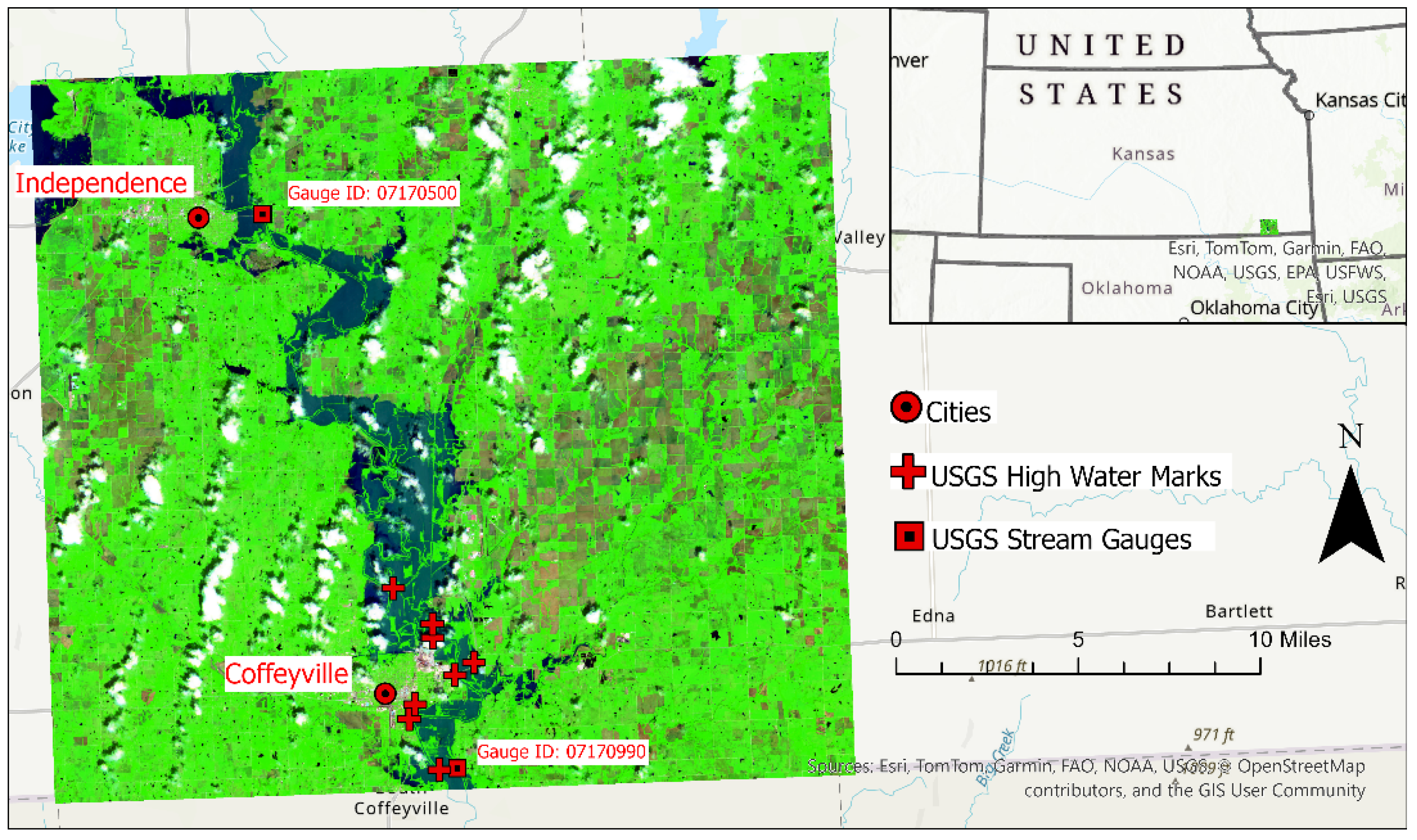
Figure 1. Study area showing the Cities of Independence and Coffeyville, the USGS stream gauges, USGS high-water marks, and the Verdigris flood event on a Sentinel-2 short-wave infrared (SWIR) image (Bands: B12, B8A, B4) captured at noon of 27 May 2019.
Remotesensing 17 03362 g001
Figure 2. Two major components in the FLDSensing method: clean water-edge detection (blue box) and stage estimation and inundation mapping (orange box).
Remotesensing 17 03362 g002
Figure 3. Map showing example unclean (red) and clean-edge pixels (green) on the NAIP imagery (a) and the Sentinel-2 SWIR imagery (b). For visualization purposes, the edge pixels have been converted to points.
Remotesensing 17 03362 g003
Figure 4. An example where two FSPs can flood two FPP edge pixels.
Remotesensing 17 03362 g004
Figure 5. Mesh generated in HEC-RAS 2D for the study area.
Remotesensing 17 03362 g005
Figure 6. Boundary conditions time series used for the flood event modeling in HEC-RAS 2D.
Remotesensing 17 03362 g006
Figure 7. Comparison of high-water marks against HEC-RAS 2D simulation for calibration of model Manning roughness values presented in Table 3.
Remotesensing 17 03362 g007
Figure 8. HEC-RAS 2D benchmark flood inundation extent and depth.
Remotesensing 17 03362 g008
Figure 9. (a) Sentinel-2 SWIR image (RGB bands: B12, B8A, B4). (b) Agreement map between Sentinel-2 and HEC-RAS 2D benchmark, where green = True Positive (TP) (correct inundation), yellow = False Positive (FP) (incorrect inundation), red = False Negative (FN) (incorrect non-inundation), gray = True Negative (TN) (correct non-inundation).
Remotesensing 17 03362 g009
Figure 10. FLDSensing results and comparison with the HEC-RAS benchmark. (a) FLDSensing depth map; (b) agreement map between FLDSensing and HEC-RAS extent maps; (c) depth difference map (FLDSensing-HEC-RAS). All maps are in NAD83 UTM zone 14N.
Remotesensing 17 03362 g010
Figure 11. FwDET depth map and comparison with HEC-RAS map. (a) FwDET depth map; (b) agreement map between FwDET and HEC-RAS extent maps; (c) depth difference map of FwDET-HEC-RAS. All maps are in NAD83 UTM zone 14N.
Remotesensing 17 03362 g011
Figure 12. FLEXTH depth map and comparison with HEC-RAS benchmark map. (a) FLEXTH depth map; (b) extent agreement map between FLEXTH and HEC-RAS extent maps; (c) depth difference map of FLEXTH-HEC-RAS. All maps are in NAD83 UTM zone 14N.
Remotesensing 17 03362 g012
Figure 13. FLDSensing results when all the FSPs are used. (a) FLDSensing depth map with all the FSPs; (b) agreement map between FLDSensing and HEC-RAS extent maps; (c) depth difference map of FLDSensing-HEC-RAS. All maps are in NAD83 UTM zone 14N.
Remotesensing 17 03362 g013
Figure 14. FLDSensing results without applying the Savitzky–Golay filter. (a) FLDSensing depth map; (b) agreement map between FLDSensing and HEC-RAS extent map; (c) depth difference map of FLDSensing-HEC-RAS. All maps are in NAD83 UTM zone 14N.
Remotesensing 17 03362 g014
Table 1. All the possible DOF combinations and their corresponding flood depths for the two FSPs.
CaseDOF (FSP1)DOF (FSP2)Flood Depth at FPP1Flood Depth at FPP2Valid?
17.58max(7.5 − 7.5, 8 − 8) = 0max(7.5 − 9, 8 − 11) = −1.5No (0, −1.5)
27.511max(7.5 − 7.5, 11 − 8) = 3max(7.5 − 9, 11 − 11) = 0Yes (3, 0)
398max(9 − 7.5, 8 − 8) = 1.5max(9 − 9, 8 − 11) = 0Yes (1.5, 0)
4911max(9 − 7.5, 11 − 8) = 3max(9 − 9, 11 − 11) = 0Yes (3, 0)
Table 2. Equations for evaluation metrics.
MetricFormulaTarget Score
Critical Success Index (CSI)CSI =   T r u e   P o s i t i v e s T r u e   P o s i t i v e s   +   F a l s e   N e g a t i v e s   +   F a l s e   P o s i t i v e s 1
Probability of Detection (POD)POD =   T r u e   P o s i t i v e s T r u e   P o s i t i v e s     +   F a l s e   N e g a t i v e s   1
False Alarm Ratio (FAR)FAR = F a l s e   P o s i t i v e s T r u e   P o s i t i v e s   + F a l s e   P o s i t i v e s 0
F1 ScoreRecall = T r u e   P o s i t i v e s T r u e   P o s i t i v e s   + F a l s e   N e g a t i v e s
Precision =   T r u e   P o s i t i v e s T r u e   P o s i t i v e s   + F a l s e   P o s i t i v e s
F1 Score =   2     P r e c i s i o n     R e c a l l P r e c i s i o n   + R e c a l l
1
Table 3. Manning’s roughness coefficient numbers used for the HEC-RAS 2D model calibration.
Land CoverRange Evaluated for Roughness CoefficientFinal Roughness Coefficient
Open water0.02–0.0450.035
Developed areas0.075–0.150.08
Barren land0.03–0.050.04
Forests/Wetlands0.08–0.20.1
Cultivated crops0.04–0.0650.05
Table 4. Performance metrics for remote sensing-based, FLDSensing, FwDET, and FLEXTH methods.
ResultsCSIPODFARF1PBIAS%RMSE (Feet)
Sentinel-2 Only0.550.560.030.71N/AN/A
FLDSensing0.890.980.090.9457.75%5.27
FwDET 2.10.380.390.070.55−61.02%7.61
FLEXTH0.810.900.110.89−29.98%3.38
Table 5. FLDSensing performance metrics with different settings.
ResultsCSIPODFARF1PBIAS%RMSE (Feet)
FLDSensing (with only mainstem)0.890.980.090.9457.75%5.27
FLDSensing (all tributaries)0.560.9980.440.72142.99%12.22
FLDSensing (without filtering)0.750.980.240.86135.69%10.06
Table 6. Savitzky–Golay filter window sizes and their performance metrics.
Window SizeF1FARPBIAS %
1010.880.21113.53
10010.880.19108.80
70010.930.1155.56%
14,0010.940.0957.75%
Disclaimer/Publisher’s Note: The statements, opinions and data contained in all publications are solely those of the individual author(s) and contributor(s) and not of MDPI and/or the editor(s). MDPI and/or the editor(s) disclaim responsibility for any injury to people or property resulting from any ideas, methods, instructions or products referred to in the content.