2C-Net: A Novel Spatiotemporal Dual-Channel Network for Soil Organic Matter Prediction Using Multi-Temporal Remote Sensing and Environmental Covariates

Highlights

What are the main findings?

• Propose a new framework for soil organic matter (SOM) mapping by combining deep learning.
• Considering multi-temporal remote sensing images (MTRSI) as multi-channel time series data to assist in SOM mapping.

What is the implication of the main finding?

• The accuracy of SOM prediction using this framework surpasses the widely used Random Forest (RF) method.
• The bare soil period after tilling is a more important time window for SOM inversion.

Abstract

Soil organic matter (SOM) is essential for ecosystem health and agricultural productivity. Accurate prediction of SOM content is critical for modern agricultural management and sustainable soil use. Existing digital soil mapping (DSM) models, when processing temporal data, primarily focus on modeling the changes in input data across successive time steps. However, they do not adequately model the relationships among different input variables, which hinders the capture of complex data patterns and limits the accuracy of predictions. To address this problem, this paper proposes a novel deep learning model, 2-Channel Network (2C-Net), leveraging sequential multi-temporal remote sensing images to improve SOM prediction. The network separates input data into temporal and spatial data, processing them through independent temporal and spatial channels. Temporal data includes multi-temporal Sentinel-2 spectral reflectance, while spatial data consists of environmental covariates including climate and topography. The Multi-sequence Feature Fusion Module (MFFM) is proposed to globally model spectral data across multiple bands and time steps, and the Diverse Convolutional Architecture (DCA) extracts spatial features from environmental data. Experimental results show that 2C-Net outperforms the baseline model (CNN-LSTM) and mainstream machine learning model for DSM, with R² = 0.524, RMSE = 0.884 (%), MAE = 0.581 (%), and MSE = 0.781 (%)². Furthermore, this study demonstrates the significant importance of sequential spectral data for the inversion of SOM content and concludes the following: for the SOM inversion task, the bare soil period after tilling is a more important time window than other bare soil periods. 2C-Net model effectively captures spatiotemporal features, offering high-accuracy SOM predictions and supporting future DSM and soil management.

1. Introduction

Soil organic matter (SOM) plays an indispensable role in sustaining soil fertility and supporting agricultural productivity, which are essential for long-term food security, especially in the face of a growing global population [1,2]. Organic matter in soils is fundamental to maintaining soil health and ensuring the sustainability of agricultural systems. In addition to improving the physical and chemical properties of soil, SOM fosters a favorable environment for crop growth and enhances nutrient availability. Moreover, SOM is a critical component of the global carbon cycle, with its accumulation contributing to carbon sequestration, a process that is integral to mitigating the impacts of climate change [3,4,5]. Therefore, accurately mapping the spatial distribution of SOM not only provides scientific evidence for agricultural production and food security, helping to formulate effective land management and conservation measures, but also contributes to assessing carbon storage capacity and supporting the implementation of climate change adaptation and mitigation strategies, ultimately ensuring the sustainability of ecosystem services.

Remote sensing technology, with its advantages of multi-dimensional information, long-term monitoring, and wide-area coverage, possesses inherent strengths in SOM mapping. It enables the rapid, accurate, and low-cost acquisition of spatial distribution maps of SOM [6,7,8,9]. Additionally, multi-temporal remote sensing image (MTRSI) data can naturally be considered as multivariate time series (MTS) data in the temporal dimension (Figure 1). The spectral bands at different time periods are likely to exhibit correlations. Therefore, this study takes into account explicitly integrated spectral information from multiple bands across the time dimension. On this basis, exploring the integration of this with deep learning (DL) techniques appears to be a natural progression. MTRSI, due to its temporal continuity, stacks remote sensing images with the same resolution from different time points, which enables change detection. As a result, it was initially widely used for tasks such as change detection and land use analysis [10,11,12]. Later, with the development of machine learning and deep learning, researchers began to use neural networks to extract dynamic features from remote sensing images, using these features as one of the bases for predicting or distinguishing soil properties [13,14,15].

Due to the high costs of manual soil sample collection, comprehensive sampling for research is impractical. Consequently, existing studies [16,17,18,19] using traditional machine learning (ML) or deep learning models typically follow a “sampling, modeling, inference” approach for indirect observation. Traditional ML models, such as Support Vector Machines (SVM) [20], Elastic Net [21], K-Nearest Neighbors (KNN) [22], and tree-based models like Random Forest [23], XGBoost [24], and LightGBM [25], are widely used in digital soil mapping (DSM). Random Forest (RF), which was designed in 2001, is particularly popular due to its ease of use, high integration, and fast training. However, even when the number of trees is set within a reasonable range, it still struggles to capture complex data patterns in certain situations [26]. When combined with remote sensing techniques for mapping, traditional mechine learning models often require expert-driven feature engineering [27,28]. In contrast, deep learning models excel at automatically learning features and optimizing networks, capturing complex patterns with less reliance on expert knowledge [29]. This places deep learning as a promising research direction for enhancing the accuracy and efficiency of DSM tasks.

The current task of soil mapping is based on Jenny’s soil formation factors and spatial variability [30,31,32]. This framework is called “SCORPAN”, which stands for soil (S), climate (C), organisms (O), relief (R), parent material (P), age (A), and nutrition (N). DSM is a rapidly developing field that uses advanced computing technologies like machine learning [33,34,35] or deep learning [36,37] to predict and map soil properties at different spatial scales. Machine learning and deep learning are providing key solutions to improve the accuracy, efficiency, and scalability of DSM. This study integrates two approaches for modeling soil organic matter (SOM), combining the advantage of the former in utilizing multi-source environmental data with the latter’s capacity to rapidly and extensively acquire soil reflectance data via remote sensing, thereby enabling more accurate and efficient spatial prediction of SOM.

In traditional machine learning methods, RF is widely used due to its ability to capture complex relationships among soil properties. For instance, some studies [16,35,38,39] utilized Random Forest models in combination with remote sensing data (e.g., satellite imagery) to predict SOC content or SOM content. Compared to deep learning, traditional machine learning’s ability to resist spatial variability is limited because it can only accept a single raster pixel value when processing spatial data [40]. At the same time, when it comes to sequential data, traditional machine learning methods like RF are limited [41].

In recent years, with the development of deep learning and the inherent advantages of CNN in processing flat data (such as images and remote sensing images), CNN has gradually been applied to the field of remote sensing. CNN was developed in 1989 by Yann LeCun and his team based on the working principles of human handwriting [42,43]. Due to the variability of its receptive field, it can capture spatial features of the ground from multiple scales using remote sensing images. Some studies [44,45] used CNN for computer vision tasks on remote sensing images (such as change detection, semantic segmentation, object detection, etc.), demonstrating its effectiveness in the field of remote sensing. At the same time, CNN has also been widely applied in the DSM field, where it can effectively extract and model spatial patterns of soil properties [46,47,48]. In research related to processing sequence data, Recurrent Neural Network (RNN) and its extensions (such as LSTM) are used as the main model or module in DSM studies [49,50,51]. However, as mentioned in this section, LSTM has limitations when dealing with multiple sequences. In addition, some studies [17,26] used mixture models as statistical tools to handle multiple subpopulations, combined with Geographic Information System (GIS), to conduct both local and overall comparative studies of soil properties. These algorithms integrate specific domain knowledge from soil science, improving the performance and interpretability of soil property prediction. Inspired by Zhang et al. [52] in soil organic carbon (SOC) mapping, this study analyzes their approach to extracting temporal dimension information, where Long Short-Term Memory (LSTM) networks [53] are employed to capture the temporal information of phenology and Enhanced Vegetation Index (EVI) variables. However, LSTM is inherently designed for processing single sequence data. While it can handle multi-sequence data through shared parameters, parallel processing, or stacking channels, it lacks a specialized mechanism to model the interactions among these sequences. This limitation prevents the model from effectively capturing the relationships among MTS data, thereby hindering the full exploitation of the latent associations among them. As a result, the model may not be capable of effectively capturing the latent patterns and interdependencies among MTRSI data in the DSM task, potentially introducing predictive bias. Furthermore, LSTM implicitly models MTS data without flexible human intervention, which can lead to overfitting, further limiting its ability to globally model MTS data.

Recently, attention mechanisms have been widely applied in deep learning. The introduction of the Transformer [54] has revolutionized the trajectory of deep learning models. This model proposes a point-wise multi-head attention mechanism for natural language processing tasks, utilizing self-attention to focus on the information currently being processed, while the cross-attention mechanism enables the decoder to directly access the information processed by the encoder. Ref. [55] leveraged cross-attention mechanisms to learn the relationships among different modalities in cross-modal learning tasks. Studies such as [56,57,58] optimized time series prediction by incorporating attention mechanisms within the Transformer framework, demonstrating outstanding performance and significant research contributions. Meanwhile, attention mechanisms have also been extended to digital soil mapping tasks. Ref. [18] introduced attention mechanisms to model spatiotemporal features in the task of predicting organic carbon content. Ref. [59] incorporated attention mechanisms within a CNN framework to model spectral data for the estimation of organic carbon content. Additionally, Ref. [60] combined positional encoding with GATConv (a graph neural network operator), which includes attention mechanisms, to better capture spatial complexity.

In summary, traditional DSM models or deep learning methods based on LSTM struggle to capture the complex interactions between multiple temporal frequency bands. To address the aforementioned challenges, this study proposes an innovative spatiotemporal 2-Channel Net (2C-Net) deep learning model for SOM prediction and mapping. 2C-Net utilizes the interaction between temporal and spatial channels to enhance feature extraction. Specifically, the temporal channel captures MTRSI data for global modeling, while the spatial channel models climate and topographic data. The model integrates SOM ground observations results with spatiotemporal data to learn the underlying complex patterns.

• The 2C-Net model is proposed and applied to SOM mapping: This study proposes a spatiotemporal 2-channel architecture that combines the advantages of cross-attention mechanism and convolutional neural networks (CNNs) to extract features of spatiotemporal information. The temporal channel extracts features from MTRSI data, while the spatial channel captures environmental covariates, such as climate and topography, to model spatial features. By integrating the information captured from both channels, the model enables efficient and accurate prediction of SOM content.
• To map MTRSI data to MTS data and perform global modeling: This study temporally sequentializes MTRSI data along the temporal dimension and maps it into MTS data. Meanwhile, we propose a novel decoder—Multi-Sequence Feature Fusion Module (MFFM)—which aims to model MTRSI from two dimensions: spectral bands and time. Unlike the LSTM that models each sequence independently, MFFM considers the relationships and interactions between different sequences.
• To enrich spatial features and perform feature extraction: This study proposes the Diverse Convolutional Architecture (DCA), which acts as the core module for spatial channels. By utilizing different convolutional kernels in the convolutional space, it effectively captures spatial information while enriching the intermediate features.

This study aims to develop and test a spatiotemporal dual-channel deep learning model (2C-Net) that integrates temporal spectral reflectance data and spatial environmental covariates to improve SOM prediction accuracy.

2. Materials and Methodology

2.1. Study Area

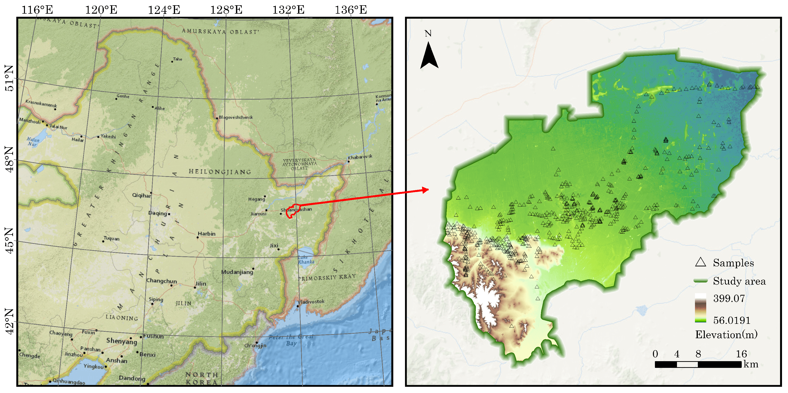
The study area is located in the Youyi Farm, Shuangyashan City, Heilongjiang Province, China (Figure 2). The farm stretches 56 km from east to west and spans 44 km from north to south, with a total cultivated area of 110,429 hectares. It is situated in a typical temperate continental monsoon climate zone, with a relatively low annual average temperature, and precipitation primarily concentrated in the summer and autumn seasons.

Youyi Farm is one of China’s largest mechanized state-owned farms and a key grain-producing area, located in the typical black soil region of Northeast China. The farm’s soil is mainly meadow soil, with small amounts of brown and black soils. The black soil layer is 40 cm to 60 cm thick. The soil is fertile and suitable for agriculture, with rice, corn, and soybeans being the main crops in the region.

2.2. Dataset

2.2.1. Temporal Data

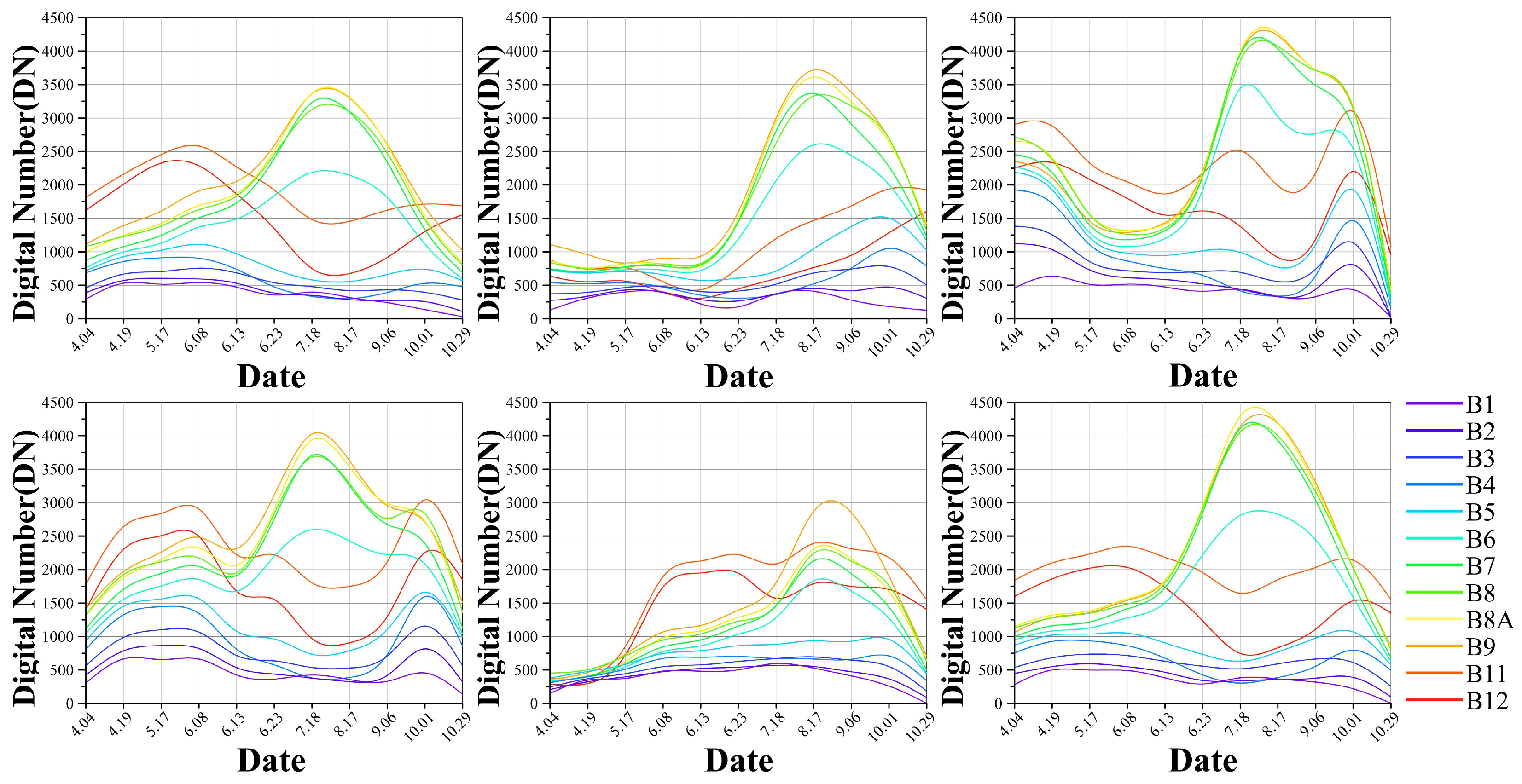
The first part of the dataset consists of atmospherical corrected, cloud-free Sentinel-2 Level-2A (L2A) MTRSI, which is well suited for soil and agricultural remote sensing analysis, and has been validated by previous studies for its effectiveness in predicting SOM [61,62,63,64]. It is obtained from the Google Earth Engine (GEE) platform (https://earthengine.google.com/, accessed on 1 February 2025), covering the period from April to October 2021; this period includes the bare soil phase (April to June), the crop growing season (June to August), and the late crop growing season (September to October), covering the soil conditions in the northeastern agricultural region of China throughout the year [16]. Figure 3 shows the MTRSI of the stitched and clipped area, with a total of 11 periods. It is clearly evident that the period before 13 June is dominated by bare soil, and from 23 June onward, crops begin to grow. All images are mosaicked using a tiling method, followed by resampling to 30 m using the nearest neighbor technique for full-band alignment.

2.2.2. Spatial Data

The second part consists of climate and topographic data for the study area (

Table 1. Key indicators of environmental covariates. CNBL refers to the channel network base level.

Various	Pixel Size (m)	Class
Annual temperature	1000	Climate
Annual precipitation	1000	Climate
Elevation	30	Terrain
CNBL	27	Terrain

). The climate data includes the annual average temperature and annual average precipitation for 2021, while the topographic data includes a 30m resolution Digital Elevation Model and channel network base level data. Previous studies [63,65,66] demonstrated that SOM content is related to climate conditions and topographical factors to some extent. The 30 m resolution Digital Elevation Model (DEM) data are obtained from the Geospatial Data Cloud platform (https://www.gscloud.cn, accessed on 1 February 2025). The annual average temperature and precipitation data of 2021 are sourced from the “China Ecological and Environmental Database” created by the Institute of Agricultural Resources and Regional Planning, Chinese Academy of Agricultural Sciences. Additionally, the channel network base level (CNBL) data are extracted using the SAGA GIS v9.2.0 software (https://saga-gis.sourceforge.io, accessed on 2 February 2025). All data are resampled to 30 m using the nearest neighbor method after clipping or mosaicking, in order to align with the remote sensing imagery data.

2.2.3. SOM Sampling Data

In this study, a total of 576 surface soil samples from different areas of paddy and dry fields were collected in 2022. The collected soil samples were air-dried and ground to particles smaller than 2 mm before analysis. The Wet Combustion Method was then used: potassium dichromate was used to oxidize the organic matter in the samples, and titration was performed to measure the unreacted oxidizing agent [67]. The SOC content was then calculated, and the SOM was obtained by multiplying SOC by a conversion factor (it is generally assumed that SOC makes up 58% of SOM by weight [68,69,70]).

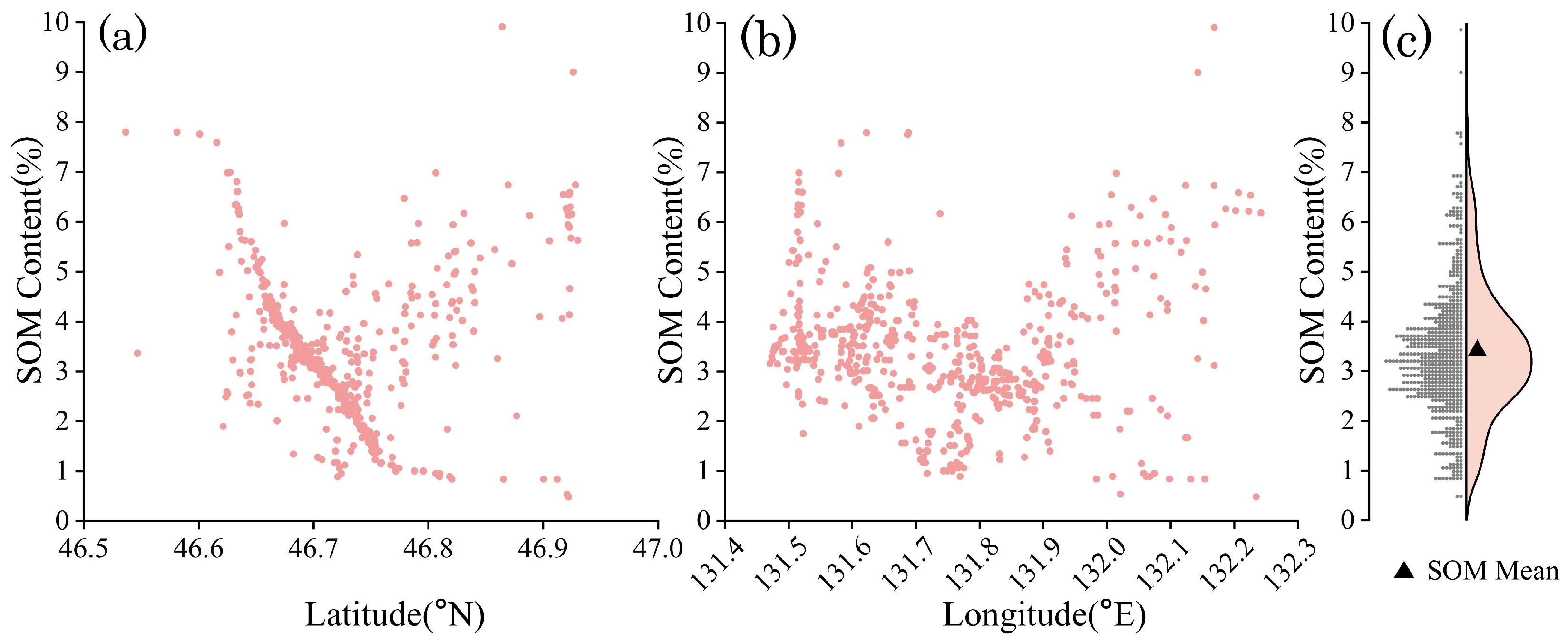
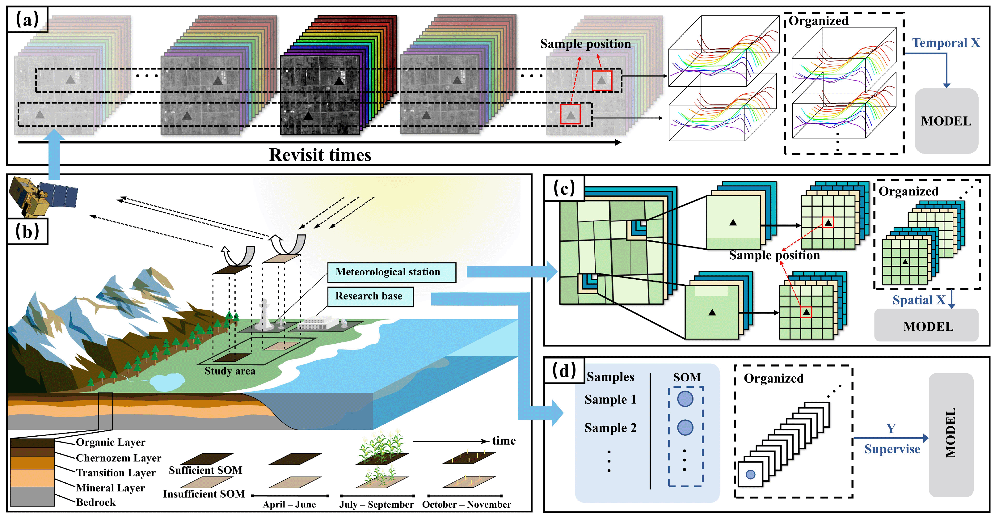
The distribution of SOM content in samples along latitude and longitude, as well as the overall distribution, is shown in Figure 4. The range is 0.48–9.91% and the mean is 3.46%. The measured SOM sample results will be input into the model and used as ground truth to supervise the training process of the model, as shown in Figure 5d.

2.3. Basic Scheme

In the context of continuous observation of a specific region over a given time period, MTRSI data naturally serve as a critical input for research. The core idea presented in this approach is to convert MTRSI data into MTS data by temporally sequentializing it (Figure 5a), thereby enabling global modeling of multiple spectral bands across both the spectral bands and temporal dimensions. When stacking climate and terrain variables along the variable dimension for modeling, the use of a single 30m resolution raster pixel value as input data did not take into account the spatial neighborhood correlation of the soil (this is also a limitation of traditional machine learning algorithms, especially in regression tasks, where they can only accept the value of a single pixel as input [40]), resulting in insufficient utilization of spatial information. By assigning different weights to the grid cells near the sample center, the influence of nearby grid cells on the modeling process can be considered (Figure 5c).

As demonstrated by [16,35,36,38], integrating the collected temporal data, spatial information, and some ground observation data for modeling represents a well-established and validated paradigm (Figure 5b).

2.4. Workflow and Architecture

2.4.1. Workflow

Figure 6 illustrates the abstract process from data acquisition to model training. Within this process, the two key components of the model are the temporal channel and the spatial channel, which are responsible for modeling the temporal and spatial data, respectively, ultimately generating the prediction results. During the training process, the model undergoes iterative optimization, continuously adjusting its parameters until the optimal state is achieved.

2.4.2. Model Architecture

Temporal and spatial information play a crucial role in assessing SOM content [3]. In this study, temporal data $X^t\in {\mathbb{R}}^{B\times T\times N}$ and spatial data $X^s\in {\mathbb{R}}^{M\times N}$ are fed into the model’s temporal and spatial channels for extraction. The temporal channel is designed to capture the temporal variation patterns of reflectance $\alpha$ across B spectral bands for each pixel, where T represents the time resolution of the spectral data and N denotes the number of samples. The spatial channel is designed to capture the data patterns of soil pixels across M spatial variables. Additionally, longitude and latitude information $X^p\in {\mathbb{R}}^{D\times N}$ is embedded as positional information into the temporal channel to enhance the model’s learning capability, where D represents the two dimensions of longitude and latitude. The following sections will introduce each part of the model. The architecture of 2C-Net is shown in Figure 7.

2.5. Temporal Channel

This study collected 11 periods of MTRSI data from April to October 2021, which are treated as MTS data. Each remote sensing image from each period is treated as one time step, and then input into the temporal channel (Figure 7a).

To explore how to better capture the data patterns of MTRSI data in the bands and temporal dimensions, this study first analyzes the approach of the CNN-LSTM architecture in processing sequential information [52,71]. This architecture uses the LSTM model to capture the temporal variations in phenology and EVI variables, which is a variant of RNN. Due to the unique memory cells and gating mechanisms of LSTM, it is widely used in traditional time series forecasting tasks and in DSM fields because it effectively captures the forward and backward dependencies in time series. A similar technique is Gated Recurrent Unit (GRU) [72], which introduces update and reset gates to process time series data. Although LSTM and GRU show strong performance in time series analysis and forecasting tasks, when these models are used for MTS data, they do not involve specialized structures to capture the relationships between different sequences. Instead, they mainly focus on the information changes of each sequence at a given time point, ignoring the interactions between different sequences. In the following sections, the LSTM used in the baseline model to process temporal features will be replaced with GRU for comparative analysis. For simplicity, this modified model will be referred to as CNN-GRU model.

Inspired by the router mechanism in CrossFormer [73], this paper proposes a novel decoder—MFFM decoder. This model facilitates the interaction of multi-sequence features across both the bands and temporal dimensions, thereby enabling global modeling across bands and time. Compared to traditional LSTM models, MFFM is more efficient in fusing MTS data, optimizing the modeling of inter-feature dependencies, and enhancing the ability to integrate information. The core objective of this method is to overcome the limitations of LSTM in modeling MTS data. This section introduces the time-channel of 2C-Net. In this section, all formulas use x to represent the variables within the time channel.

2.5.1. Encoder

In deep learning, the encoder serves to extract a fixed-form feature representation from the raw input. As the data flows through the encoder, the raw input information is abstracted and transformed into higher-level features. These features are then retrieved and processed by the decoder. In this paper, the encoder is kept relatively simple, with the aim of maximizing the extraction of input information while avoiding unnecessary complexity. It is composed of value embedding and coordinate embedding.

• Value embedding: The band information of the raw input $X^t$ is passed through a linear layer to obtain MTS vector $x_i^{val}(i\in \{1,2,\dots ,N\})$, with N representing the number of samples and “$val$” is the abbreviation for “value”. The linear layer, as one of the fundamental building blocks in neural networks, is responsible for performing linear transformations of the data. During the subsequent training process, through backpropagation and optimization, the model adjusts its parameters so that the linear layer can optimally map the input information. To keep the encoder simple, this paper does not stack multiple linear layers at this point. A ReLU activation function is applied to introduce non-linearity, thereby enhancing the model’s expressive capability. The process of value embedding can be expressed as follows:

  $$x_i^{val}=ReLU\left(Linear\left(X^t\right)\right)$$

  (1)
• Coordinate embedding: For each spectral band data, after embedding it as a vector $x_i^{val}$, we incorporate the longitude and latitude information of all samples, denoted as $X^p\in {\mathbb{R}}^{D\times N}$, into the embedding process. This serves two purposes: on the one hand, it provides unique positional information for each spectral band, and on the other hand, it enhances the relevance with the subsequent decoder’s retrieval head. In the fields of natural language processing and computer vision, positional embedding is a widely adopted technique. This approach provides models with positional information for sequences or image patches, thereby improving the model’s understanding of the input [54,74,75]. Similarly, in this paper, after embedding different bands’ information as N vectors $\left\{x_1^{val},x_2^{val},\dots ,x_N^{val}\right\}$, the latitude and longitude information of each sample is treated as default-encoded and embedded into N vectors $\left\{x_1^p,x_2^p,\dots ,x_N^p\right\}$ (as shown in Equation (2)). N represents the number of samples and “p” is the abbreviation for “position”. These vectors are then integrated with the band information by concatenation (as shown in Equation (3)), resulting in the output of the encoder: $x_i(i\in \{1,2,\dots ,N\})$.

  $$x_i^p=ReLU\left(Linear\left(X^p\right)\right)$$

  (2)

  $$x_i=Concat\left(x_i^{val},x_i^p\right)$$

  (3)

2.5.2. MFFM Decoder

In deep learning, decoders typically interpret or map the features extracted by the encoder through a series of transformations. This paper proposes a novel decoder, MFFM, which injects the spectral information captured by the encoder into retrieval heads, organized by spectral bands, and then performs fusion to enable global modeling of multispectral information. The core principle of MFFM is as follows: the coordinate information $X^p$ of each sample point is embedded and rearranged into B retrieval heads $\left\{h_{i,1},h_{i,2},\dots ,h_{i,B}\right\}(i\in \{1,2,\dots ,N\})$, N represents the number of samples, and B represents the number of retrieval heads ($\mathit{B}$ bands match $\mathit{B}$ retrieval heads). Each retrieval head corresponds to a rearranged target $\left\{{\mathit{x}}_{\mathit{i},\mathit{1}},{\mathit{x}}_{\mathit{i},\mathit{2}},\dots ,{\mathit{x}}_{\mathit{i},\mathit{B}}\right\}(\mathit{i}\in \{\mathit{1},\mathit{2},\dots ,\mathit{N}\})$ from the encoder. After each retrieval head processes the corresponding target, these retrieval heads will be fed into router mechanism for cross-band modeling, ultimately producing the global modeling output. The working process of MFFM can be divided into three stages: decoder initialization, head retrieval, and head fusion. These paragraphs provide detailed explanations of the working mechanism of MFFM.

• Decoder initialization: For each sample $\mathit{i}$$(\mathit{i}\in \{\mathit{1},\mathit{2},\dots ,\mathit{N}\left\}\right)$, the coordinate information ${\mathit{X}}^{\mathit{p}}$ of all sample points is embedded and rearranged into $\mathit{B}$ vectors $\left\{{\mathit{h}}_{\mathit{i},\mathit{1}},{\mathit{h}}_{\mathit{i},\mathit{2}},\dots ,{\mathit{h}}_{\mathit{i},\mathit{B}}\right\}$. $\mathit{N}$ represents the number of samples, $\mathit{B}$ represents the number of retrieval heads, and “$\mathit{h}$” is the abbreviation for “head”. This process is as follows:

  $$\left\{{\mathit{h}}_{\mathit{i},\mathit{1}},{\mathit{h}}_{\mathit{i},\mathit{2}},\dots ,{\mathit{h}}_{\mathit{i},\mathit{B}}\right\}=\mathit{Rearrange}\left(\mathit{ReLU}\left(\mathit{Linear}\left({\mathit{X}}^{\mathit{p}}\right)\right)\right)$$

  (4)
• Head retrieval: Before performing the retrieval, each encoder output ${\mathit{x}}_{\mathit{i}}(\mathit{i}\in \{\mathit{1},\mathit{2},\dots ,\mathit{N}\})$ is rearranged to align with the corresponding set of retrieval heads from the decoder, resulting in the retrieval targets ${\mathit{x}}_{\mathit{i},\mathit{j}}(\mathit{i}\in \{\mathit{1},\mathit{2},\dots ,\mathit{N}\})$ for the retrieval heads. This process is as follows:

  $$\left\{{\mathit{x}}_{\mathit{i},\mathit{1}},{\mathit{x}}_{\mathit{i},\mathit{2}},\dots ,{\mathit{x}}_{\mathit{i},\mathit{B}}\right\}=\mathit{Rearrange}\left({\mathit{x}}_{\mathit{i}}\right)$$

  (5)
  Subsequently, for each sample $\mathit{i}$$(\mathit{i}\in \{\mathit{1},\mathit{2},\dots ,\mathit{N}\left\}\right)$, retrieval heads ${\mathit{h}}_{\mathit{i},\mathit{j}}(\mathit{j}\in \{\mathit{1},\mathit{2},\dots ,\mathit{B}\})$ and the corresponding retrieval targets ${\mathit{x}}_{\mathit{i},\mathit{j}}(\mathit{j}\in \{\mathit{1},\mathit{2},\dots ,\mathit{B}\})$, the $\mathit{B}$ retrieval heads $\left\{{\mathit{h}}_{\mathit{i},\mathit{1}},{\mathit{h}}_{\mathit{i},\mathit{2}},\dots ,{\mathit{h}}_{\mathit{i},\mathit{B}}\right\}$ are used as queries $\mathit{q}$, and the $\mathit{B}$ retrieval targets $\left\{{\mathit{x}}_{\mathit{i},\mathit{1}},{\mathit{x}}_{\mathit{i},\mathit{2}},\dots ,{\mathit{x}}_{\mathit{i},\mathit{B}}\right\}$ are used as keys $\mathit{k}$ and values $\mathit{v}$. A cross-attention operation is then performed and then we get $\mathit{B}$ retrieval results ${\mathit{h}}_{\mathit{i},\mathit{j}}^{\mathbf{input}}(\mathit{j}\in \{\mathit{1},\mathit{2},\dots ,\mathit{B}\})$, which are injected with encoder information; $\mathit{input}$ means that it will be input vector of router mechanism. This process is as follows:

  $${\mathit{h}}_{\mathit{i},\mathit{j}}^{\mathit{input}}=\mathit{CrossAttention}\left({\mathit{h}}_{\mathit{i},\mathit{j}},{\mathit{x}}_{\mathit{i},\mathit{j}},{\mathit{x}}_{\mathit{i},\mathit{j}}\right)$$

  (6)
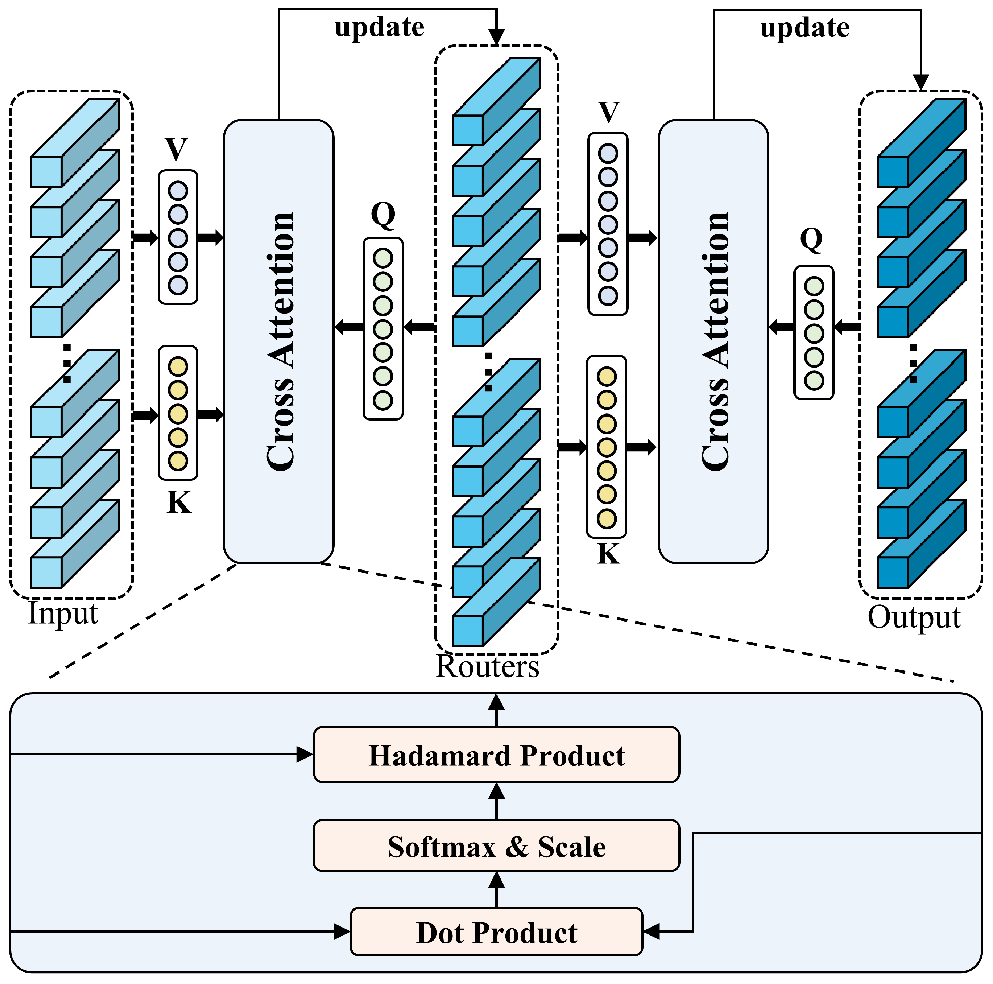
• Head fusion: The retrieval results will be treated as input and fed into the router mechanism, a technique proposed by [73] for MTS forecasting tasks. The router mechanism operates by establishing a routing layer that stores temporary information between input and output vectors of the same dimensionality. In CrossFormer, this layer accepts the input information, integrates it, and then distributes it to the output recipients, resulting in an architecture of ${\mathit{D}}^{\mathit{I}}\times {\mathit{D}}^{\mathit{R}}\times {\mathit{D}}^{\mathit{O}}$, where ${\mathit{D}}^{\mathit{R}}<{\mathit{D}}^{\mathit{I}}={\mathit{D}}^{\mathit{O}}$. ${\mathit{D}}^{\mathit{R}}$, ${\mathit{D}}^{\mathit{I}}$ and ${\mathit{D}}^{\mathit{O}}$ represent the dimensions of the router, input, and output in the router mechanism, respectively. This mechanism significantly reduces the computational complexity of intermediate vectors through the intermediate routing layer. However, compared to typical MTS forecasting tasks, datasets in the DSM domain have fewer variables, making computational complexity not the primary concern of this study (but it still needs to be considered, as will be mentioned in Section 3.2.2). In this work, by reversing the approach, we set ${\mathit{D}}^{\mathit{R}}>{\mathit{D}}^{\mathit{I}}={\mathit{D}}^{\mathit{O}}$ (as shown in Figure 8), where increasing the number of intermediate routers enhances the richness of feature representation while minimizing information loss.
  For each sample $\mathit{i}$, the $\mathit{B}$ retrieval results ${\mathit{h}}_{\mathit{i},\mathit{j}}^{\mathrm{input}}(\mathit{j}\in \{\mathit{1},\mathit{2},\dots ,\mathit{B}\})$ injected with encoder information are first used as the $\mathit{k}$ and $\mathit{v}$, while the initial vectors from the router layer serve as the queries $\mathit{q}$. The first cross-attention operation is then performed among these components (as shown in Equation (7)), yielding initial fused temporary vectors ${\mathit{h}}_{\mathit{i},\mathit{r}}^{\mathrm{router}}\left(\mathit{r}\in \left\{\mathit{1},\mathit{2},\dots ,{\mathit{D}}^{\mathit{R}}\right\}\right)$. Subsequently, the temporary router layer vectors ${\mathit{h}}_{\mathit{i},\mathit{r}}^{\mathrm{router}}$ are used as the $\mathit{k}$ and $\mathit{v}$, and the retrieval results ${\mathit{h}}_{\mathit{i},\mathit{j}}^{\mathrm{input}}$ are used as $\mathit{q}$ in the second cross-attention operation (as shown in Equation (8)), and we get the final fused vectors ${\mathit{h}}_{\mathit{i},\mathit{j}}^{\mathit{output}}(\mathit{j}\in \{\mathit{1},\mathit{2},\dots ,\mathit{B}\})$ after mutual interaction. $\mathit{B}$ represent the number of retrieval heads.

  $${\mathit{h}}_{\mathit{i},\mathit{r}}^{\mathit{router}}=\mathit{CrossAttention}\left({\mathit{h}}_{\mathit{i},\mathit{r}}^{\mathit{router}},{\mathit{h}}_{\mathit{i},\mathit{j}}^{\mathit{input}},{\mathit{h}}_{\mathit{i},\mathit{j}}^{\mathit{input}}\right)$$

  (7)

  $${\mathit{h}}_{\mathit{i},\mathit{j}}^{\mathit{output}}=\mathit{CrossAttention}\left({\mathit{h}}_{\mathit{i},\mathit{j}}^{\mathit{input}},{\mathit{h}}_{\mathit{i},\mathit{r}}^{\mathit{router}},{\mathit{h}}_{\mathit{i},\mathit{r}}^{\mathit{router}}\right)$$

  (8)
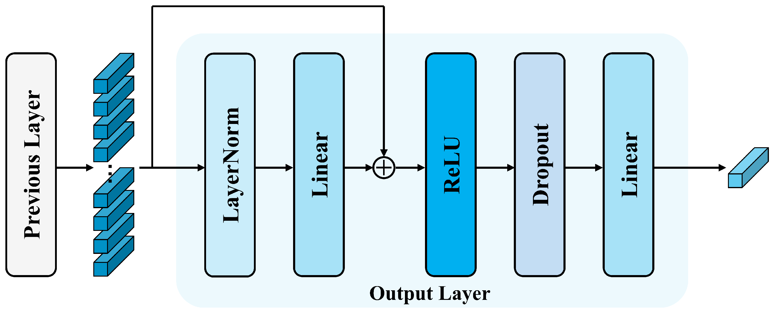
  The $\mathit{B}$ fused results are then passed into the output layer (Figure 9), followed by a reshape operation and a fully connected layer (FC), which produces the final output ${\mathit{y}}^{\mathit{t}}$ for the temporal channel. This process is as follows:

  $${\mathit{y}}^{\mathit{t}}=\mathit{FC}\left(\mathit{Reshape}\left(\mathit{OutputLayer}\left({\mathit{h}}_{\mathit{i},\mathit{j}}^{\mathit{output}}\right)\right)\right)$$

  (9)

2.6. Spatial Channel

The spatial channel of the model is primarily composed of two DCA blocks, each containing convolutional layers with different parameters (e.g., kernel size, stride, etc.) as outlined in

Table 2. The different convolutional layer parameters for two DCA blocks, including input channels (I.C.), output channels (O.C.), stride, padding, and activation.

Block	Kernel	I.C.	O.C.	Stride	Padding	Activation
DCA Block 1	3 × 3	4	24	1	1	ReLU
	3 × 3	24	24	1	1	ReLU
	4 × 4	24	32	1	2	ReLU
	1 × 1	32	32	1	-	ReLU
DCA Block 2	2 × 2	32	32	1	1	ReLU
	1 × 1	32	16	1	-	ReLU

. Climate and terrain data are treated as spatial data ${\mathit{X}}^{\mathit{s}}$ and fed into spatial channel (Figure 7b). In this section, we use $\mathit{x}$ to represent the valuable within the spatial channel.

Specifically, the first DCA block includes two 3 × 3 convolutional layers, one 4 × 4 convolutional layer, one 1 × 1 convolutional layer, and one max-pooling layer. The second DCA block comprises one 2 × 2 convolutional layer, one 1 × 1 convolutional layer, and one max-pooling layer. Additionally, a ReLU activation function follows each convolutional layer, introducing non-linear transformations.

The DCA blocks enhance feature representation by increasing the intermediate channel dimensions, thereby enriching feature diversity and robustness while reducing information loss. Furthermore, this study introduces 1 × 1 convolutions [76]. Compared to other convolutional kernels, the 1 × 1 convolution offers lower computational cost, while effectively integrating features from different channels by adjusting the number of channels, thus generating a global feature representation. As an intermediate layer in the network, the 1 × 1 convolution has the advantage of being flexibly inserted at various locations within the network. Similar to other convolutional layers, applying an activation function after the 1 × 1 convolution introduces non-linear transformations, thereby enhancing the model’s representational capacity.

After feature extraction through two layers of DCA blocks, the result will be reshaped and further processed via fully connected layers (FC), ultimately producing the spatial-channel output ${\mathit{y}}^{\mathit{s}}$. This process is as follows:

$${\mathit{y}}^{\mathit{s}}=\mathit{FC}\left(\mathit{Reshape}\left(\mathit{DCA}\left(\mathit{x}\right)\right)\right)$$

(10)

3. Results

To evaluate the accuracy of the model’s fit for SOM content, we employed a ten-fold cross-validation approach for training all models. We use RMSE (Root Mean Square Error), MAE, MSE, R² and RPIQ as evaluation metrics. Lower RMSE, MAE, and MSE represent more accurate model fitting. Higher R² and RPIQ represents the better ability of the model to explain the data. These metrics provide a comprehensive evaluation of the model’s performance across various aspects. All models use the same training and testing datasets, preprocessing methods, and data normalization techniques. All models are trained on the same NVIDIA GeForce RTX 2080 Ti GPU,(manufactured by NVIDIA Corporation, American) and grid search is used to determine the optimal hyperparameters. All deep learning-based models are trained with a batch size of 128, a step decay learning rate of adam optimizer (starts at 0.0001 and halves every 100 epochs), and for 500 epochs. Early stopping is applied to save the best model.

This paper chooses Huber Loss as the loss function [77], as it combines the advantages of Mean Squared Error (MSE) Loss and Mean Absolute Error (MAE) Loss, offering improved robustness to outliers. The definition of Huber Loss is as follows:

$$\mathit{Loss}=\left\{\begin{array}{cc}{\displaystyle \frac{\mathit{1}}{\mathit{2}}}{(\mathit{y}-\widehat{\mathit{y}})}^{\mathit{2}},\hfill & \mathit{if} |\mathit{y}-\widehat{\mathit{y}}|\le \mathit{\delta }\hfill \\ \mathit{\delta }\left(|\mathit{y}-\widehat{\mathit{y}}|-{\displaystyle \frac{\mathit{1}}{\mathit{2}}}\mathit{\delta }\right),\hfill & \mathit{otherwise}\hfill \end{array}\right.$$

(11)

where $\mathit{y}$ represents the true value, $\widehat{\mathit{y}}$ denotes the predicted value, and $\mathit{\delta }$ is a non-negative constant used as a threshold. In this study, $\mathit{\delta }$ is set to 1.

3.1. Compare with Other Models’ Performance

To demonstrate the superiority of the 2C-Net model, a comparison is made with several typical machine learning methods and baseline models (

Table 3. The results of machine learning and deep learning models are shown, including RMSE, MAE, MSE, R², and RPIQ metrics. The optimal values are highlighted in bold. Our model shows significant improvement over the CNN-LSTM model in all metrics (the values in parentheses show the improvement of 2C-Net compared to the baseline CNN-LSTM).

Models		RMSE (%)	MAE (%)	MSE (%)2	R2	RPIQ
Machine learning	KNN [22]	1.181	0.869	1.395	0.151	1.44
	Elastic Net [21]	1.110	0.796	1.232	0.249	1.51
	LightGBM [25]	1.141	0.791	1.302	0.206	1.50
	SVM [20]	1.116	0.824	1.246	0.292	1.48
	XGBoost [24]	1.056	0.678	1.115	0.321	1.67
	RF [23]	0.955	0.610	0.912	0.451	1.59
Deep learning	CNN-LSTM [52]	0.982	0.704	0.964	0.412	1.65
	CNN-GRU	0.977	0.678	0.955	0.421	1.67
	2C-Net (Ours)	0.884	0.581	0.781	0.524	1.89

), including RF [23], XGBoost [24], Support Vector Machine (SVM) [20], Elastic Net [21], K-Nearest Neighbors (KNN) [22], LightGBM [25], and the baseline model CNN-LSTM [52] used in this study. Additionally, a supplementary comparison is made by replacing CNN-LSTM with CNN-GRU. From the results presented in Table 3, it can be observed that the 2C-Net model outperforms the other models across all four evaluation metrics. Compared to the baseline CNN-LSTM model, the 2C-Net model achieves a 27% improvement in R², a 19% reduction in MSE, a 17% reduction in MAE, and a 10% reduction in RMSE, thereby validating the effectiveness of the 2C-Net model.

This paper will focus on the results obtained from the Random Forest model and three deep learning models. A scatter plot of the predictions in Figure 10 is presented. The model with GRU replacing LSTM shows a more accurate prediction trend compared to the CNN-LSTM model, with its slope being closer to 1. The Random Forest model outperforms both the CNN-LSTM model and the CNN-GRU model in terms of accuracy. The 2C-Net model demonstrates superior performance in both the general prediction trend and individual prediction accuracy compared to other models. These results are consistent with the results presented in Table 3.

3.2. Ablation Study

3.2.1. Analysis of the Impact of Various Modules on Results

In this section, this paper progressively introduces key components including coordinate embedding (CE), DCA, and MFFM into the network to obtain different variants. Then, we replace Huber Loss to conduct ablation experiments and validate the potential benefits of these components. The results are presented in

Table 4. Ablation study of various key components in 2C-Net based on RMSE (%), MAE (%), MSE (%)², R², and RPIQ metrics. Bold text indicates the best result.

Models	RMSE	MAE	MSE	R2	RPIQ
2C-Net w/o MFFM DCA CE	1.112	0.824	1.237	0.347	1.47
2C-Net w/o MFFM DCA	1.004	0.720	1.009	0.386	1.61
2C-Net w/o MFFM	0.996	0.677	0.992	0.402	1.65
2C-Net with all	0.884	0.581	0.781	0.524	1.89

and

Table 5. Impact of different loss functions on model prediction outcomes, with RMSE (%), MAE (%), MSE (%)², R², and RPIQ metrics. Bold text indicates the methods used in this study.

Loss Function	RMSE	MAE	MSE	R2	RPIQ
MAE Loss	0.925	0.615	0.856	0.478	1.71
MSE Loss	0.922	0.635	0.851	0.482	1.77
Huber Loss	0.884	0.581	0.781	0.524	1.89

. In each variant presented in Table 4, Huber Loss is retained (its effectiveness will be separately validated in Table 5), and the entire model is retrained and evaluated.

• 2C-Net w/o MFFM DCA CE: In this part, all components are removed from the complete network, and only the two 2 × 2 convolutional layers in the baseline CNN-LSTM architecture are used to extract climate and terrain data, while an MLP is employed to extract spectral data.
• 2C-Net w/o MFFM DCA: In order to compare 1. and validate the effectiveness of the CE component, the MFFM and DCA components are removed from the complete network, and the CE component is added in this part.
• 2C-Net w/o MFFM: In order to compare 2. and validate the effectiveness of the DCA component, the MFFM component is removed from the complete network, while the DCA component and CE are added in this part.
• 2C-Net(with all components): In order to compare 3. and validate the effectiveness of the MFFM component, all components are added in this part.

3.2.2. Evaluation of Router Mechanism’s Hyperparameter

This part tests the impact of the number of routers in the routing mechanism on model performance, as well as the effects of model complexity and computational overhead.

As shown in Figure 11a, when the number of routers reaches 15, the model performance outperforms that when the number of routers is less than the number of bands. This supports the hypothesis presented in this study: by increasing the number of routers in the routing mechanism, the relationship ${\mathit{D}}^{\mathit{R}}>{\mathit{D}}^{\mathit{I}}={\mathit{D}}^{\mathit{O}}$ can be achieved, thereby providing the model with richer feature representation capabilities and effectively reducing the extent of information loss. This adjustment not only enhances the model’s expressive power but also optimizes the information transfer process.

Due to the involvement of the cross-attention mechanism, the number of routers not only affects the complexity of the hidden features but also significantly influences the model’s parameter count and computational overhead. As shown in Figure 11a,b, when the number of routers approaches 100, although the model performance is similar to that of when the number of routers is 15, the memory consumption, parameter count, and MACs (multiply–accumulate operations) all increase significantly. Notably, the MACs even double compared to the case with 15 routers. This impact is expected to further escalate when applied to large-scale datasets. Considering the balance between optimal performance and resource consumption, this study selects the number of routers to be 15.

3.2.3. Evaluation of Channel Fusion Methods

There are two methods for channel integration: concatenation and direct addition. This study conducts a test on these methods (

Table 6. Impact of different channel fusion methods on model prediction outcomes of 2C-Net, with RMSE (%), MAE (%), MSE (%)², R², and RPIQ Metrics. Bold text indicates the methods used in this study.

Methods	RMSE	MAE	MSE	R2	RPIQ
Add	0.918	0.632	0.842	0.487	1.78
Concat	0.884	0.581	0.781	0.524	1.89

), and the results indicate that concatenation outperforms direct addition by a significant margin.

3.3. Visualization

3.3.1. Visualization of Different Models’ Mapping Results

The objective of DSM is to leverage GIS and remote sensing technologies to accurately visualize complex soil properties, making it more accessible for understanding and application. In this study, the model is trained using the collected samples, and the optimal model parameters are selected. Subsequently, all image data are fused into a single TIFF file, which contains spectral information and environmental covariate data. This file is then input into the model for prediction. The final step involves clipping and colorizing the predicted results to generate the final spatial distribution map of SOM content. The spatial distribution predictions of organic matter content using four models—RF, CNN-LSTM, CNN-GRU, and 2C-Net—are presented in Figure 12. Detailed analysis will be presented in Section 4.1.

3.3.2. Visualization of Spectral Feature Importance

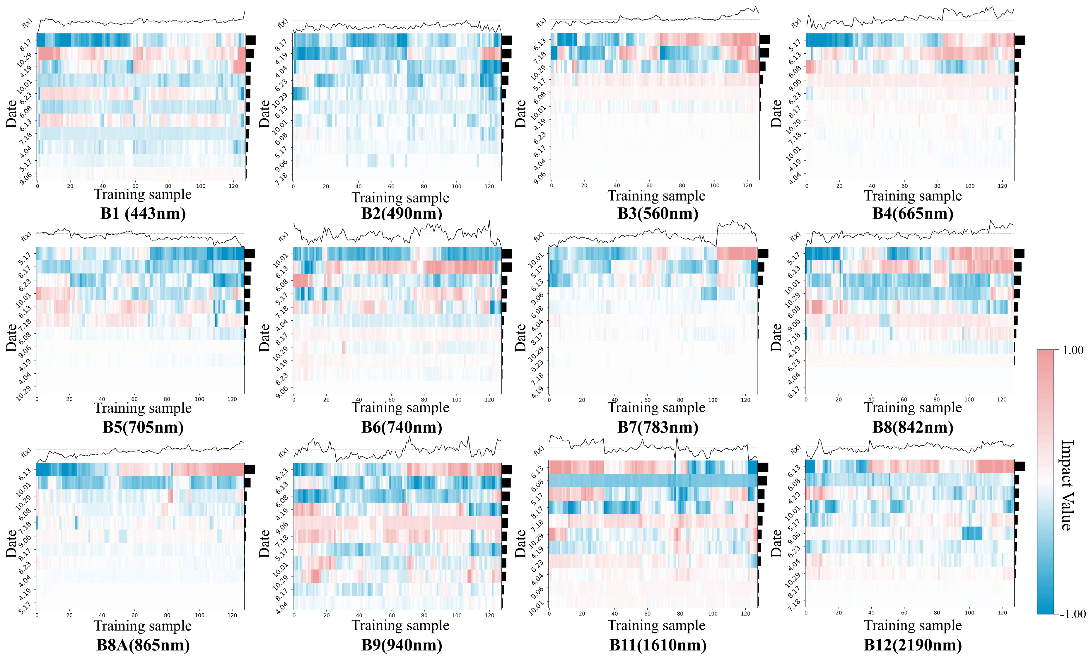
The SHAP method [78], based on cooperative game theory, can be used to interpret the outputs of deep learning models. It explains the model’s decisions by comparing the difference between the actual input and the baseline input, and incorporating the gradient information at each layer. Deep SHAP calculates the contribution of each feature to the model’s output, thereby enhancing the interpretability of deep learning models. In this study, the SHAP method is incorporated into the temporal channel to evaluate the contribution of spectral and temporal dimensions of MTRSI data (Figure 13). For different bands of MTRSI, images at different time periods are treated as individual features (rows), and the Shapley value is calculated for each feature. A positive value indicates a positive contribution of the feature to the prediction, while a negative value represents a negative contribution. It is important to note that a negative contribution does not mean the feature has no effect on the model’s final prediction, but rather that the variation in the feature’s value is negatively correlated with the predicted outcome. We will analyze the details from spectral and temporal perspectives in Section 4.3.

4. Discussion

4.1. Mapping Result

From Figure 12, it can be seen that the SOM distribution maps from all models show that areas with higher SOM content are located in the southwest and northeast parts of the study area, while areas with lower SOM content are in the central part, forming a band that runs through the area. This overall trend is consistent with the SOM distribution at the sampling points (Figure 12e). The results of traditional machine learning and deep learning differ when considering spatial variability, which may be due to the fact that the way CNN extracts spatial information is different from traditional machine learning (Figure 12a(i)–d(i)). However, the local mapping results obtained from different deep learning models may also vary, which could be due to the fact that they consider different factors when modeling spatial data (Figure 12b(ii),c(ii)). All four models can effectively predict areas with very low values (Figure 12a(iii)–d(iii)), further confirming the consistency of the overall trend in the maps generated by the four models.

4.2. Uncertainty of Mapping Result

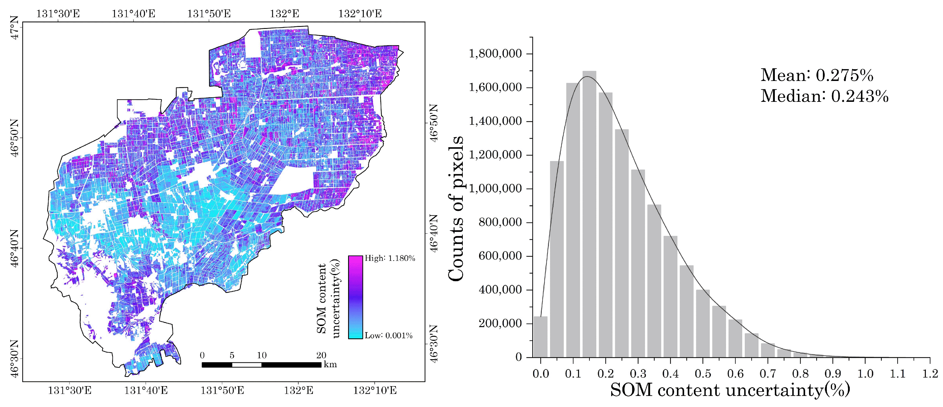
We computed the standard deviation of the 10-fold cross-validation results and generated an uncertainty map for the 2C-Net mapping result (Figure 14). The results revealed that the mean uncertainty was 0.275% and the median uncertainty was 0.243%. This indicates that the overall results generated by 2C-Net mapping demonstrate a high level of stability.

4.3. Feature Importance

4.3.1. From the Perspective of the Spectral Dimension

There are significant differences in the overall contribution of different spectral bands to the model’s prediction results. Among them, the B1, B2, B5, B6, B8, B9, B11, and B12 bands make more noticeable contributions to the model (Figure 13). It is worth noting that the B1 band (443 nm) and the B9 band (940 nm) of Sentinel-2A, which are rarely used in traditional SOM mapping studies, play an important role in the prediction model. The B1 band is widely used for water body detection, and aerosol and cloud detection in the atmosphere, while the B9 band is primarily used for detecting water vapor in the atmosphere and atmospheric correction. Our hypothesis is that by combining the B1 and B9 bands with other bands, the impact of aerosols and water vapor in the atmosphere on ground reflectance can be corrected. Deep learning, with its ability to automatically capture features, integrates this complex relationship into the model. In future tasks, we will focus on this aspect and use appropriate methods to validate our hypothesis.

4.3.2. From the Perspective of the Temporal Dimension

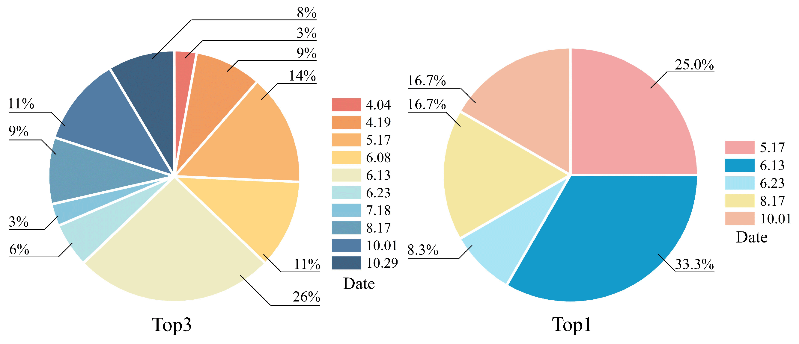
According to Figure 3, it can be seen that before 6.13, the soil was in a bare soil period. Also, based on our field survey, local residents tilled the soil between April and May, exposing the humus in the soil surface to the air. The visualization results from Figure 15 show that in the top three important date images, 5.17, 6.8, and 6.13 account for 51.4% of the contribution, all of which are in the bare soil period after tilling. In the top panel with the most important date images, 5.17 and 6.13 contribute 58.3%. Previous studies have shown that images from the bare soil period are important [35,62], and the results in this paper confirm that the bare soil period after tilling is a more critical time window for inverting SOM content. The current work [16,17,19] may achieve improved predictive accuracy by placing greater emphasis on post-plowing imagery data, such as by assigning it higher weight in the final model, thereby enhancing the overall performance.

4.4. Limitations of This Study and Prospects

Due to resource constraints, this study focused solely on validating the model’s effectiveness and drawing preliminary conclusions based on data collected from Youyi Farm in northeastern China. Future work will aim to enhance the model’s transferability to other regions, thereby facilitating its broader application in subsequent research. Additionally, since deep learning techniques are data-driven, the model’s accuracy could be further improved with larger datasets. We also intend to explore the potential integration of hyperspectral data to improve model performance.

Moreover, deep learning methods, by eliminating the need for feature engineering, do not rely on expert prior knowledge, which simplifies the modeling process. However, this also complicates the supervision of the model’s decision-making process. Furthermore, the “black box” nature of deep learning limits our ability to interpret feature relationships. For instance, in this study, we are unable to further verify the hypothesis that combining the Sentinel-2A B1 and B9 bands with other spectral bands might effectively mitigate the impact of aerosols and water vapor on atmospheric correction. The exploration of these aspects will be a key focus in our future research efforts.

5. Conclusions

This paper proposes an innovative spatiotemporal 2-channel network (2C-Net) for soil organic matter (SOM) prediction and demonstrates its superiority in predicting the SOM content in the typical black soil region of Northeast China. By integrating Sentinel-2 MTRSI with environmental covariates such as climate and topography, 2C-Net significantly improves the accuracy of SOM prediction compared to the baseline CNN-LSTM model. Furthermore, compared to the traditional model mechine learning in digital soil mapping (DSM), key metrics including R², RMSE, MAE, MSE show significant improvements. In this study, the Multi-Sequence Feature Fusion Module (MFFM) effectively captures spectral information from different bands in multi-temporal remote sensing imagery (MTRSI), while the Diverse Convolutional Architecture (DCA) structure more effectively extracts spatial information. The effectiveness of key components in the network is further validated through ablation experiments. Additionally, the importance of multispectral reflectance information in both the spectral and temporal dimensions is assessed, quantifying the contribution of MTRSI to model performance in these two dimensions, leading us to conclude that for the SOM inversion task, the bare soil image after tilling represents a more critical time window than other bare soil imagery. Overall, the 2C-Net model, by capturing rich spatiotemporal features, provides an accurate and reliable solution for SOM content prediction, with broad application prospects, particularly in DSM and sustainable soil management decision-making.

References

1. Tiessen, H.; Cuevas, E.; Chacon, P. The role of soil organic matter in sustaining soil fertility. Nature 1994, 371, 783–785. [Google Scholar] [CrossRef]
2. Luo, C.; Zhang, X.; Wang, Y.; Men, Z.; Liu, H. Regional soil organic matter mapping models based on the optimal time window, feature selection algorithm and Google Earth Engine. Soil Tillage Res. 2022, 219, 105325. [Google Scholar] [CrossRef]
3. Guo, L.; Sun, X.; Fu, P.; Shi, T.; Dang, L.; Chen, Y.; Linderman, M.; Zhang, G.; Zhang, Y.; Jiang, Q.; et al. Mapping soil organic carbon stock by hyperspectral and time-series multispectral remote sensing images in low-relief agricultural areas. Geoderma 2021, 398, 115118. [Google Scholar] [CrossRef]
4. Bhattacharyya, S.S.; Ros, G.H.; Furtak, K.; Iqbal, H.M.; Parra-Saldívar, R. Soil carbon sequestration–An interplay between soil microbial community and soil organic matter dynamics. Sci. Total Environ. 2022, 815, 152928. [Google Scholar] [CrossRef] [PubMed]
5. Bashir, O.; Ali, T.; Baba, Z.A.; Rather, G.; Bangroo, S.; Mukhtar, S.D.; Naik, N.; Mohiuddin, R.; Bharati, V.; Bhat, R.A. Soil organic matter and its impact on soil properties and nutrient status. In Microbiota and Biofertilizers, Vol 2: Ecofriendly Tools for Reclamation of Degraded Soil Environs; Springer: Cham, Switzerland, 2021; pp. 129–159. [Google Scholar]
6. Hamzehpour, N.; Shafizadeh-Moghadam, H.; Valavi, R. Exploring the driving forces and digital mapping of soil organic carbon using remote sensing and soil texture. CATENA 2019, 182, 104141. [Google Scholar] [CrossRef]
7. Luo, C.; Zhang, W.; Zhang, X.; Liu, H. Mapping the soil organic matter content in a typical black-soil area using optical data, radar data and environmental covariates. Soil Tillage Res. 2024, 235, 105912. [Google Scholar] [CrossRef]
8. Wang, X.; Zhang, F.; Kung, H.-T.; Johnson, V.C. New methods for improving the remote sensing estimation of soil organic matter content (SOMC) in the Ebinur Lake Wetland National Nature Reserve (ELWNNR) in northwest China. Remote Sens. Environ. 2018, 218, 104–118. [Google Scholar] [CrossRef]
9. Zhou, T.; Geng, Y.; Ji, C.; Xu, X.; Wang, H.; Pan, J.; Bumberger, J.; Haase, D.; Lausch, A. Prediction of soil organic carbon and the C: N ratio on a national scale using machine learning and satellite data: A comparison between Sentinel-2, Sentinel-3 and Landsat-8 images. Sci. Total Environ. 2021, 755, 142661. [Google Scholar] [CrossRef]
10. Du, P.; Liu, S.; Xia, J.; Zhao, Y. Information fusion techniques for change detection from multi-temporal remote sensing images. Inf. Fusion 2013, 14, 19–27. [Google Scholar] [CrossRef]
11. Jianya, G.; Haigang, S.; Guorui, M.; Qiming, Z. A review of multi-temporal remote sensing data change detection algorithms. Int. Arch. Photogramm. Remote Sens. Spat. Inf. Sci. 2008, 37, 757–762. [Google Scholar]
12. Du, P.; Li, X.; Cao, W.; Luo, Y.; Zhang, H. Monitoring urban land cover and vegetation change by multi-temporal remote sensing information. Min. Sci. Technol. 2010, 20, 922–932. [Google Scholar] [CrossRef]
13. Zhong, L.; Hu, L.; Zhou, H. Deep learning based multi-temporal crop classification. Remote Sens. Environ. 2019, 221, 430–443. [Google Scholar] [CrossRef]
14. Wang, L.; Tian, Y.; Yao, X.; Zhu, Y.; Cao, W. Predicting grain yield and protein content in wheat by fusing multi-sensor and multi-temporal remote-sensing images. Field Crops Res. 2014, 164, 178–188. [Google Scholar] [CrossRef]
15. Duan, M.; Song, X.; Liu, X.; Cui, D.; Zhang, X. Mapping the soil types combining multi-temporal remote sensing data with texture features. Comput. Electron. Agric. 2022, 200, 107230. [Google Scholar] [CrossRef]
16. Luo, C.; Zhang, W.; Zhang, X.; Liu, H. Mapping of soil organic matter in a typical black soil area using Landsat-8 synthetic images at different time periods. CATENA 2023, 231, 107336. [Google Scholar] [CrossRef]
17. Zang, D.; Zhao, Y.; Luo, C.; Zhang, S.; Dai, X.; Li, Y.; Liu, H. Improving the accuracy of soil organic matter mapping in typical Planosol areas based on prior knowledge and probability hybrid model. Soil Tillage Res. 2025, 246, 106358. [Google Scholar] [CrossRef]
18. Meng, X.; Bao, Y.; Luo, C.; Zhang, X.; Liu, H. A new methodology for establishing an SOC content prediction model that is spatiotemporally transferable at multidecadal and intercontinental scales. ISPRS J. Photogramm. Remote Sens. 2024, 218, 531–550. [Google Scholar] [CrossRef]
19. Zhang, X.; Zhang, G.; Zhang, S.; Ai, H.; Han, Y.; Luo, C.; Liu, H. A novel model for mapping soil organic matter: Integrating temporal and spatial characteristics. Ecol. Inform. 2024, 84, 102923. [Google Scholar] [CrossRef]
20. Cortes, C.; Vapnik, V. Support-vector networks. Mach. Learn. 1995, 20, 273–297. [Google Scholar] [CrossRef]
21. Zou, H.; Hastie, T. Regularization and variable selection via the elastic net. J. R. Stat. Soc. Ser. B Stat. Methodol. 2005, 67, 301–320. [Google Scholar] [CrossRef]
22. Cover, T.; Hart, P. Nearest neighbor pattern classification. IEEE Trans. Inf. Theory 1967, 13, 21–27. [Google Scholar] [CrossRef]
23. Breiman, L. Random forests. Mach. Learn. 2001, 45, 5–32. [Google Scholar] [CrossRef]
24. Chen, T.; Guestrin, C. XGBoost: A scalable tree boosting system. In Proceedings of the 22nd ACM SIGKDD International Conference on Knowledge Discovery and Data Mining, San Francisco, CA, USA, 13–17 August 2016; pp. 785–794. [Google Scholar]
25. Ke, G.; Meng, Q.; Finley, T.; Wang, T.; Chen, W.; Ma, W.; Ye, Q.; Liu, T.Y. LightGBM: A highly efficient gradient boosting decision tree. In Proceedings of the 31st International Conference on Neural Information Processing Systems, Long Beach, CA, USA, 4–9 December 2017; Volume 30. [Google Scholar]
26. Meng, X.; Bao, Y.; Zhang, X.; Luo, C.; Liu, H. A long-term global Mollisols SOC content prediction framework: Integrating prior knowledge, geographical partitioning, and deep learning models with spatio-temporal validation. Remote Sens. Environ. 2025, 318, 114592. [Google Scholar] [CrossRef]
27. Kattenborn, T.; Leitloff, J.; Schiefer, F.; Hinz, S. Review on Convolutional Neural Networks (CNN) in vegetation remote sensing. ISPRS J. Photogramm. Remote Sens. 2021, 173, 24–49. [Google Scholar] [CrossRef]
28. Archana, R.; Jeevaraj, P.E. Deep learning models for digital image processing: A review. Artif. Intell. Rev. 2024, 57, 11. [Google Scholar] [CrossRef]
29. Odebiri, O.; Odindi, J.; Mutanga, O. Basic and deep learning models in remote sensing of soil organic carbon estimation: A brief review. Int. J. Appl. Earth Obs. Geoinf. 2021, 102, 102389. [Google Scholar] [CrossRef]
30. Jenny, H. Factors of Soil Formation: A System of Quantitative Pedology; Courier Corporation: North Chelmsford, MA, USA, 1994. [Google Scholar]
31. Sindayihebura, A.; Ottoy, S.; Dondeyne, S.; Van Meirvenne, M.; Van Orshoven, J. Comparing digital soil mapping techniques for organic carbon and clay content: Case study in Burundi’s central plateaus. CATENA 2017, 156, 161–175. [Google Scholar] [CrossRef]
32. Chen, S.; Arrouays, D.; Mulder, V.L.; Poggio, L.; Minasny, B.; Roudier, P.; Libohova, Z.; Lagacherie, P.; Shi, Z.; Hannam, J.; et al. Digital mapping of GlobalSoilMap soil properties at a broad scale: A review. Geoderma 2022, 409, 115567. [Google Scholar] [CrossRef]
33. Wadoux, A.M.C.; Minasny, B.; McBratney, A.B. Machine learning for digital soil mapping: Applications, challenges and suggested solutions. Earth-Sci. Rev. 2020, 210, 103359. [Google Scholar] [CrossRef]
34. Taghizadeh-Mehrjardi, R.; Hamzehpour, N.; Hassanzadeh, M.; Heung, B.; Goydaragh, M.G.; Schmidt, K.; Scholten, T. Enhancing the accuracy of machine learning models using the super learner technique in digital soil mapping. Geoderma 2021, 399, 115108. [Google Scholar] [CrossRef]
35. Zhang, Y.; Luo, C.; Zhang, Y.; Gao, L.; Wang, Y.; Wu, Z.; Zhang, W.; Liu, H. Integration of bare soil and crop growth remote sensing data to improve the accuracy of soil organic matter mapping in black soil areas. Soil Tillage Res. 2024, 244, 106269. [Google Scholar] [CrossRef]
36. Meng, X.; Bao, Y.; Luo, C.; Zhang, X.; Liu, H. SOC content of global Mollisols at a 30 m spatial resolution from 1984 to 2021 generated by the novel ML-CNN prediction model. Remote Sens. Environ. 2024, 300, 113911. [Google Scholar] [CrossRef]
37. Liu, Q.; He, L.; Guo, L.; Wang, M.; Deng, D.; Lv, P.; Wang, R.; Jia, Z.; Hu, Z.; Wu, G.; et al. Digital mapping of soil organic carbon density using newly developed bare soil spectral indices and deep neural network. CATENA 2022, 219, 106603. [Google Scholar] [CrossRef]
38. Kong, D.; Chu, N.; Luo, C.; Liu, H. Analyzing spatial distribution and influencing factors of soil organic matter in cultivated land of northeast China: Implications for black soil protection. Land 2024, 13, 1028. [Google Scholar] [CrossRef]
39. Luo, C.; Zhang, W.; Meng, X.; Yu, Y.; Zhang, X.; Liu, H. Mapping the soil organic matter content in Northeast China considering the difference between dry lands and paddy fields. Soil Tillage Res. 2024, 244, 106270. [Google Scholar] [CrossRef]
40. Chauhan, N.K.; Singh, K. A review on conventional machine learning vs deep learning. In Proceedings of the 2018 International Conference on Computing, Power and Communication Technologies (GUCON), Greater Noida, India, 28–29 September 2018; pp. 347–352. [Google Scholar]
41. Nagendra, B.; Singh, G. Comparing ARIMA, linear regression, random forest, and LSTM for time series forecasting: A study on item stock predictions. In Proceedings of the 2023 4th IEEE Global Conference for Advancement in Technology (GCAT), Bangalore, India, 6–8 October 2023; pp. 1–8. [Google Scholar]
42. LeCun, Y.; Boser, B.; Denker, J.S.; Henderson, D.; Howard, R.E.; Hubbard, W.; Jackel, L.D. Backpropagation applied to handwritten zip code recognition. Neural Comput. 1989, 1, 541–551. [Google Scholar] [CrossRef]
43. Kuang, X.; Wang, F.; Hernandez, K.M.; Zhang, Z.; Grossman, R.L. Accurate and rapid prediction of tuberculosis drug resistance from genome sequence data using traditional machine learning algorithms and CNN. Sci. Rep. 2022, 12, 2427. [Google Scholar] [CrossRef]
44. Sagar, A.S.; Chen, Y.; Xie, Y.; Kim, H.S. MSA R-CNN: A comprehensive approach to remote sensing object detection and scene understanding. Expert Syst. Appl. 2024, 241, 122788. [Google Scholar] [CrossRef]
45. Yao, M.; Zhang, Y.; Liu, G.; Pang, D. SSNet: A novel transformer and CNN hybrid network for remote sensing semantic segmentation. IEEE J. Sel. Top. Appl. Earth Obs. Remote Sens. 2024, 17, 3023–3037. [Google Scholar] [CrossRef]
46. Radočaj, D.; Gašparović, M.; Jurišić, M. Open remote sensing data in digital soil organic carbon mapping: A review. Agriculture 2024, 14, 1005. [Google Scholar] [CrossRef]
47. Bao, Y.; Yao, F.; Meng, X.; Wang, J.; Liu, H.; Wang, Y.; Liu, Q.; Zhang, J.; Mouazen, A.M. A fine digital soil mapping by integrating remote sensing-based process model and deep learning method in Northeast China. Soil Tillage Res. 2024, 238, 106010. [Google Scholar] [CrossRef]
48. Zhao, X.; Heiden, U.; Karlshöfer, P.; Xiong, Z.; Zhu, X.X. Soil Organic Carbon Retrieval from DESIS Images by CNN. In Proceedings of the EGU General Assembly Conference Abstracts, Vienna, Austria, 14–19 April 2024; p. 9731. [Google Scholar]
49. Senanayake, S.; Pradhan, B.; Alamri, A.; Park, H.J. A new application of deep neural network (LSTM) and RUSLE models in soil erosion prediction. Sci. Total Environ. 2022, 845, 157220. [Google Scholar] [CrossRef] [PubMed]
50. Huang, F.; Zhang, Y.; Zhang, Y.; Shangguan, W.; Li, Q.; Li, L.; Jiang, S. Interpreting Conv-LSTM for spatio-temporal soil moisture prediction in China. Agriculture 2023, 13, 971. [Google Scholar] [CrossRef]
51. Li, Q.; Zhang, C.; Shangguan, W.; Li, L.; Dai, Y. A novel local-global dependency deep learning model for soil mapping. Geoderma 2023, 438, 116649. [Google Scholar] [CrossRef]
52. Zhang, L.; Cai, Y.; Huang, H.; Li, A.; Yang, L.; Zhou, C. A CNN-LSTM model for soil organic carbon content prediction with long time series of MODIS-based phenological variables. Remote Sens. 2022, 14, 4441. [Google Scholar] [CrossRef]
53. Hochreiter, S.; Schmidhuber, J. Long short-term memory. Neural Comput. 1997, 9, 1735–1780. [Google Scholar] [CrossRef]
54. Vaswani, A.; Shazeer, N.; Parmar, N.; Uszkoreit, J.; Jones, L.; Gomez, A.N.; Kaiser, Ł.; Polosukhin, I. Attention is all you need. In Proceedings of the 31st International Conference on Neural Information Processing Systems, Long Beach, CA, USA, 4–9 December 2017; Volume 30. [Google Scholar]
55. Lu, J.; Batra, D.; Parikh, D.; Lee, S. Vilbert: Pretraining task-agnostic visiolinguistic representations for vision-and-language tasks. In Proceedings of the 33rd International Conference on Neural Information Processing Systems, Vancouver, BC, Canada, 8–14 December 2019; Volume 32. [Google Scholar]
56. Wu, H.; Xu, J.; Wang, J.; Long, M. Autoformer: Decomposition transformers with auto-correlation for long-term series forecasting. Adv. Neural Inf. Process. Syst. 2021, 34, 22419–22430. [Google Scholar]
57. Zhou, T.; Ma, Z.; Wen, Q.; Wang, X.; Sun, L.; Jin, R. Fedformer: Frequency enhanced decomposed transformer for long-term series forecasting. In Proceedings of the International Conference on Machine Learning (PMLR), Baltimore, MD, USA, 17–23 July 2022; pp. 27268–27286. [Google Scholar]
58. Liu, Y.; Hu, T.; Zhang, H.; Wu, H.; Wang, S.; Ma, L.; Long, M. itransformer: Inverted transformers are effective for time series forecasting. arXiv 2023, arXiv:2310.06625. [Google Scholar]
59. Zhao, W.; Wu, Z.; Yin, Z.; Li, D. Attention-based CNN ensemble for soil organic carbon content estimation with spectral data. IEEE Geosci. Remote Sens. Lett. 2022, 19, 1–5. [Google Scholar] [CrossRef]
60. Zhao, W.; Efremova, N. Soil organic carbon estimation from climate-related features with graph neural network. arXiv 2023, arXiv:2311.15979. [Google Scholar] [CrossRef]
61. Luo, C.; Wang, Y.; Zhang, X.; Zhang, W.; Liu, H. Spatial prediction of soil organic matter content using multiyear synthetic images and partitioning algorithms. CATENA 2022, 211, 106023. [Google Scholar] [CrossRef]
62. Luo, C.; Zhang, W.; Zhang, X.; Liu, H. Mapping soil organic matter content using Sentinel-2 synthetic images at different time intervals in Northeast China. Int. J. Digit. Earth 2023, 16, 1094–1107. [Google Scholar] [CrossRef]
63. He, X.; Yang, L.; Li, A.; Zhang, L.; Shen, F.; Cai, Y.; Zhou, C. Soil organic carbon prediction using phenological parameters and remote sensing variables generated from Sentinel-2 images. CATENA 2021, 205, 105442. [Google Scholar] [CrossRef]
64. Guo, L.; Fu, P.; Shi, T.; Chen, Y.; Zeng, C.; Zhang, H.; Wang, S. Exploring influence factors in mapping soil organic carbon on low-relief agricultural lands using time series of remote sensing data. Soil Tillage Res. 2021, 210, 104982. [Google Scholar] [CrossRef]
65. Querejeta, J.I.; Schlaeppi, K.; López-García, Á.; Ondoño, S.; Prieto, I.; van Der Heijden, M.G.; del Mar Alguacil, M. Lower relative abundance of ectomycorrhizal fungi under a warmer and drier climate is linked to enhanced soil organic matter decomposition. New Phytol. 2021, 232, 1399–1413. [Google Scholar] [CrossRef] [PubMed]
66. Pouladi, N.; Gholizadeh, A.; Khosravi, V.; Borůvka, L. Digital mapping of soil organic carbon using remote sensing data: A systematic review. CATENA 2023, 232, 107409. [Google Scholar] [CrossRef]
67. Walkley, A.; Black, I.A. An examination of the Degtjareff method for determining soil organic matter, and a proposed modification of the chromic acid titration method. Soil Sci. 1934, 37, 29–38. [Google Scholar] [CrossRef]
68. Körschens, M.; Weigel, A.; Schulz, E. Turnover of soil organic matter (SOM) and long-term balances—tools for evaluating sustainable productivity of soils. Z. Pflanzenernährung Bodenkd. 1998, 161, 409–424. [Google Scholar] [CrossRef]
69. Chen, Y.; Liu, K.; Hu, N.; Lou, Y.; Wang, F.; Wang, Y. Biochemical composition of soil organic matter physical fractions under 32-year fertilization in Ferralic Cambisol. Carbon Res. 2023, 2, 1. [Google Scholar] [CrossRef]
70. Zhou, Y.; Hartemink, A.E.; Shi, Z.; Liang, Z.; Lu, Y. Land use and climate change effects on soil organic carbon in North and Northeast China. Sci. Total Environ. 2019, 647, 1230–1238. [Google Scholar] [CrossRef]
71. Dong, Z.; Yao, L.; Bao, Y.; Zhang, J.; Yao, F.; Bai, L.; Zheng, P. Prediction of soil organic carbon content in complex vegetation areas based on CNN-LSTM model. Land 2024, 13, 915. [Google Scholar] [CrossRef]
72. Cho, K.; Van Merriënboer, B.; Gulcehre, C.; Bahdanau, D.; Bougares, F.; Schwenk, H.; Bengio, Y. Learning phrase representations using RNN encoder-decoder for statistical machine translation. arXiv 2014, arXiv:1406.1078. [Google Scholar] [CrossRef]
73. Zhang, Y.; Yan, J. Crossformer: Transformer utilizing cross-dimension dependency for multivariate time series forecasting. In Proceedings of the Eleventh International Conference on Learning Representations, Kigali, Rwanda, 1–5 May 2023. [Google Scholar]
74. Carion, N.; Massa, F.; Synnaeve, G.; Usunier, N.; Kirillov, A.; Zagoruyko, S. End-to-end object detection with transformers. In Proceedings of the European Conference on Computer Vision, Glasgow, UK, 23–28 August 2020; Springer: Cham, Switzerland, 2020; pp. 213–229. [Google Scholar]
75. Dosovitskiy, A.; Beyer, L.; Kolesnikov, A.; Weissenborn, D.; Zhai, X.; Unterthiner, T.; Dehghani, M.; Minderer, M.; Heigold, G.; Gelly, S.; et al. An image is worth 16x16 words: Transformers for image recognition at scale. arXiv 2020, arXiv:2010.11929. [Google Scholar]
76. Lin, M.; Chen, Q.; Yan, S. Network in network. arXiv 2013, arXiv:1312.4400. [Google Scholar]
77. Huber, P.J. Robust estimation of a location parameter. In Breakthroughs in Statistics: Methodology and Distribution; Springer: New York, NY, USA, 1992; pp. 492–518. [Google Scholar]
78. Lundberg, S.M.; Lee, S.I. A unified approach to interpreting model predictions. In Proceedings of the 31st International Conference on Neural Information Processing Systems, Long Beach, CA, USA, 4–9 December 2017; Volume 30. [Google Scholar]
Figure 1. From a time-series perspective, the spectral information of different positions of soil samples exhibits significant diversification within the multi-spectral data, and different spectral bands contain rich associative information. Different colors represent the different Sentinel-2 bands.
Remotesensing 17 03358 g001
Figure 2. Schematic of the study area location and the distribution of samples.
Remotesensing 17 03358 g002
Figure 3. The MTRSI for different periods spanning from April to October within the study area.
Remotesensing 17 03358 g003
Figure 4. SOM content distribution. (a) Distribution of SOM content in the north–south direction. (b) Distribution of SOM content in the east–west direction. (c) Density distribution of SOM content.
Remotesensing 17 03358 g004
Figure 5. Schematic of the modeling process based on MTRSI data, climate, topography, and ground truth data. (a) MTRSI data, which can be regarded as MTS data, is input into the model’s temporal channel. (b) Soil is divided into three phases: bare soil (with no crop cover on the surface), crop growing season (with crop cover on the surface), and maturation (with crop root systems covering the surface), with distinct spectral reflectance values for each. The MTRSI data covers these phases. (c) Climate and topography data, providing spatial information, are input into the model’s spatial channel. (d) SOM sampling data, obtained from soil samples and organic matter analysis, are used to supervise model training.
Remotesensing 17 03358 g005
Figure 6. Upon the acquisition and preprocessing of the data (upper section), the temporal and spatial data are input into the model’s temporal and spatial channels for feature extraction. Subsequently, the loss value is calculated using the loss function, which contributes to the model’s optimization and iterative refinement process.
Remotesensing 17 03358 g006
Figure 7. The model’s architecture of 2C-Net. (a) The model’s temporal channel for extracting temporal features of spectral information. (b) The model’s spatial channel for extracting spatial features of climate and terrain. (c) The part of two channels’ integration and predicting.
Remotesensing 17 03358 g007
Figure 8. Schematic diagram of the routing mechanism. By using the cross-attention mechanism, the routing mechanism achieves the fusion and distribution of intermediate features, thereby enriching the representation of the intermediate features. Q, K, and V correspond to the query, key, and value components, respectively, within the context of the cross-attention mechanism.
Remotesensing 17 03358 g008
Figure 9. The structure of the output layer in the temporal channel. Through this layer, the intermediate features of the model are mapped to the appropriate dimensionality.
Remotesensing 17 03358 g009
Figure 10. The scatter plots of predictions from four different models—RF, CNN-LSTM, CNN-GRU, and 2C-Net—are shown. In these plots, the diagonal line representing the linear fit indicates the overall prediction performance. The closer the slope (m) is to 1 and the intercept (b) is to 0, the higher the overall prediction accuracy. The dark-colored bands around the diagonal line represent the 95% confidence interval, while the lighter bands on the outer edges denote the 95% prediction interval. Narrower bands signify higher prediction accuracy for individual samples.
Remotesensing 17 03358 g010
Figure 11. The impact of the number of routers on model performance, complexity, and computational overhead. (a) The performance of models with varying numbers of routers in terms of RMSE, MAE, MSE, and R2 metrics. When the routers are set to 15, the result is optimal (red dashed box). (b) The performance of models with varying numbers of routers in terms of memory allocation, parameter count, and MACs (multiply–accumulate operations). We select 15 routers (red dashed box).
Remotesensing 17 03358 g011
Figure 12. The mapping results of the four models for SOM in the study area and the distribution of sample data on the plane used to supervise the model’s training progression. (a) 2C-Net, (b) CNN-GRU, (c) CNN-LSTM, (d) RF, (e) distribution of sample SOM data on the plane. The mapping results and sample display use the same color scale for easy comparison (the color scale on the left corresponds to the sample data distribution, and the color scale on the right corresponds to the mapping results).
Remotesensing 17 03358 g012
Figure 13. Visualization of the impact of MTRSI data on model predictions in the band and temporal dimensions using the SHAP method. The red areas represent positive contributions to the model, while the blue areas indicate negative contributions. The impact value (Shapley value) reflects the magnitude of the contribution.
Remotesensing 17 03358 g013
Figure 14. The uncertainty distribution of 2C-Net mapping results (left) and the statistical values of uncertainty for all pixels (right).
Remotesensing 17 03358 g014
Figure 15. Based on Figure 13, the statistical analysis of the importance of MTRSI data across the temporal dimension is presented. The top 3 panel shows the proportion of image data from different dates that contribute the top 3 to each spectral band, reflecting the more importantimage dates for each band. The top 1 panel shows the proportion of image data from different dates that contribute the most to each spectral band, reflecting the most important image dates for each band.
Remotesensing 17 03358 g015