Abstract
Rapid and efficient evaluation of cultivated land quality in black soil regions at the farm scale using remote sensing techniques is crucial for resource protection. However, current studies face challenges in developing convenient and reliable models that directly leverage raw spectral reflectance. Therefore, this study develops and validates a deep learning framework specifically for this task. The framework first selects remote sensing images from typical periods using a Random Forest model in Google Earth Engine (GEE). Subsequently, the raw spectral reflectance data from these images, without any transformation into vegetation indices, are directly input into an optimized BO-Stacking-TabNet model. This model is enhanced through a two-step Stacking ensemble process and a Bayesian optimization algorithm. A case study at Shuanghe Farm in Northeast China shows that (1) compared to the BO-Stacking-TabNet model using vegetation indices as input, the BO-Stacking-TabNet model based on spectral reflectance as the input indicator achieved an improvement of 10.62% in Accuracy, 1.55% in Precision, 11.05% in Recall, and 10.18% in F1-score. (2) Compared to the original TabNet model, the BO-Stacking-TabNet model optimized by the two-step Stacking process and Bayesian optimization algorithm improved Accuracy by 2.13%, Precision by 12.59%, Recall by 1.83%, and F1-score by 2.19%. These results demonstrate the reliability of the new farm-scale black soil region cultivated land evaluation method we proposed. The method provides significant references for future research on cultivated land quality assessment at the farm scale in terms of remote sensing image data processing and model construction.
1. Introduction
Cultivated land is the foundation of human survival and development, and black soil region cultivated land, known for its fertility and suitability for crop cultivation, has become an extremely rare and valuable soil resource among all types of cultivated land [1,2,3]. However, in some regions of the world, particularly in Northeast China, the quality of black soil region cultivated land has significantly deteriorated due to large-scale over-cultivation and insufficient awareness of its protection [4,5,6]. Northeast China’s black soil region is one of the three major black soil regions in the world and also serves as a primary base for commercial grain supply in China [7,8]. In Northeast China, state-owned farms manage vast areas of cultivated land and play a crucial role in agricultural production [9,10]. At the same time, the Chinese government has increasingly emphasized the protection and sustainable utilization of black soil region cultivated land in recent years, introducing a series of policy documents and laws to safeguard these resources [11,12]. State-owned farms, managed by the government, naturally bear the responsibility for protecting black soil region resources and ensuring the sustainable development and utilization of black soil region cultivated land. To protect black soil region cultivated land effectively, it is essential to understand its current condition. Evaluating the quality of cultivated land serves as the foundation for state-owned farms to scientifically manage, effectively protect, and precisely enhance the quality of cultivated land. Therefore, state-owned farms have an urgent need for cultivated land quality assessment at the farm scale. By understanding the distribution of cultivated land quality, state-owned farms can adopt more targeted measures to improve and enhance the quality of the land. However, traditional methods of evaluating cultivated land quality primarily rely on soil sampling, laboratory analysis, expert surveys, scoring, data modeling, and GIS, which require considerable time, labor, and financial resources [13,14,15]. Therefore, utilizing satellite remote sensing to quickly and conveniently assess the quality of cultivated land has great practical significance.
Currently, research on cultivated land quality assessment based on remote sensing primarily focuses on multi-source data fusion. For example, studies by Pullanagari et al. [16], Wang et al. [17], Binte Mostafiz et al. [18], and Li et al. [19] have conducted cultivated land quality assessments by integrating satellite remote sensing indicators with data such as topography and meteorological information. Li et al. [20] conducted cultivated land quality assessments by combining soil indicators from field surveys, such as organic matter and pH values, with remote sensing indicators like vegetation index. These studies gather data from various online sources as indicators for land quality evaluation, replacing part or all of the soil’s physical and chemical indicators traditionally collected manually. A new system of indicators is then constructed to assess the quality of the cultivated land. Some studies have used traditional mathematical models to assess cultivated land quality based on remote sensing indicator systems. For example, Duan et al. [21] used the index method to calculate land quality grades. Other researchers have applied machine learning methods around remote sensing-based indicator systems. Liu et al. [22] established a land quality indicator system based on satellite-derived indicators using the Pressure-State-Response (PSR) framework proposed by Dumanski and Pier [23] and assessed land quality using the GA-BPNN model. Zhou et al. [24] evaluated land quality from multi-source data using the RNN algorithm. Although these studies provide valuable insights, they require the collection and processing of multiple remote sensing datasets before the evaluation process can begin. Additionally, many studies still rely on traditional modeling methods for the use of remote sensing indicators. While some have adopted machine learning techniques, the research into machine learning models remains insufficient, particularly in the area of remote sensing spectral data-based machine learning models, which lacks deeper exploration.
Current research on cultivated land quality assessment driven by single-source remote sensing spectral data is still in the exploratory stage. Some studies have utilized two types of satellite remote sensing data for this purpose. For example, Xia et al. [25] estimated the distribution of land quality using a machine learning model driven by crop growth time series spectral data, based on Landsat 8 and MODIS satellite remote sensing data. Some studies have used a single satellite remote sensing dataset to assess cultivated land quality. For example, Zhuang et al. [26] established a link between the distribution of land quality and the net primary productivity (NPP) indicator derived from Landsat single-source remote sensing imagery. Similarly, Ma et al. [27] used the MODIS-based Vegetation Photosynthesis Model (VPM) to calculate the gross primary productivity (GPP) and assess the productivity of cultivated land. However, these studies still require the spectral data extracted from remote sensing images to be further processed into derived remote sensing reflectance indicators, which demands considerable time and effort. Therefore, a research avenue worth exploring is to develop a cultivated land quality assessment model based directly on spectral reflectance data from single-source satellite remote sensing imagery, without the need to generate derived spectral indicators. However, these studies still require the spectral data extracted from remote sensing images to be further processed into derived remote sensing reflectance indicators, which demands considerable time and effort.
In recent years, deep learning has achieved significant progress in precision agriculture and remote sensing interpretation. Various architectures have been widely applied to tasks such as land use classification, crop identification, and yield estimation. For instance, Convolutional Neural Networks (CNNs) like U-Net and DeepLabv3+ excel at processing spatial context from images, making them ideal for pixel-level semantic segmentation [28,29]. Recurrent Neural Networks (RNNs), particularly Long Short-Term Memory (LSTM) networks, have proven advantageous for analyzing multi-temporal remote sensing data and capturing time-series features like crop phenology [30]. Furthermore, the Transformer architecture, especially the Vision Transformer (ViT), has emerged as a powerful new paradigm, showing great potential in remote sensing image analysis [31].
However, it is crucial to note that these models are predominantly designed for image data, excelling at extracting spatial patterns or temporal sequences. When the evaluation unit shifts from ‘pixels’ to the ‘plot’ or ‘farm’ scale, the input data is often aggregated into a tabular format (e.g., one row per plot containing mean reflectance values for multiple spectral bands). In such tabular data-driven scenarios, directly applying models designed for images may not be optimal, as the intra-plot spatial texture information has been averaged out. This motivates the exploration of deep learning models specifically designed for high-performance learning on tabular data.
TabNet is one such model, architected with built-in feature selection and interpretability for tabular data [32]. It emulates decision tree-like behavior through a sequential attention mechanism, making it highly effective for tabular feature processing. Although TabNet and ensemble techniques like Stacking have been applied in some remote sensing tasks, such as crop mapping and soil property estimation [33,34], their combined and optimized application within a framework for farm-scale cultivated land quality assessment—an ordinal classification problem using raw multi-temporal spectral reflectance directly—has not been systematically validated.
Therefore, the main contributions of this study are as follows:
(1) We validate the effectiveness of using raw multi-temporal spectral reflectance directly for CLQ assessment. This approach simplifies the data preprocessing pipeline and achieves superior accuracy compared to conventional methods that rely on derived vegetation indices.
(2) We develop and optimize a tailored BO-Stacking-TabNet framework for farm-scale CLQ assessment. We systematically demonstrate its high performance on this tabular classification task and comprehensively benchmark it against various baseline models.
(3) We propose and apply a data-driven methodology for optimal imagery selection. By leveraging a Random Forest model on the GEE platform, we objectively identify the most suitable periods for assessment, providing a quantifiable basis for temporal data selection.
2. Materials and Methods
2.1. Study Area
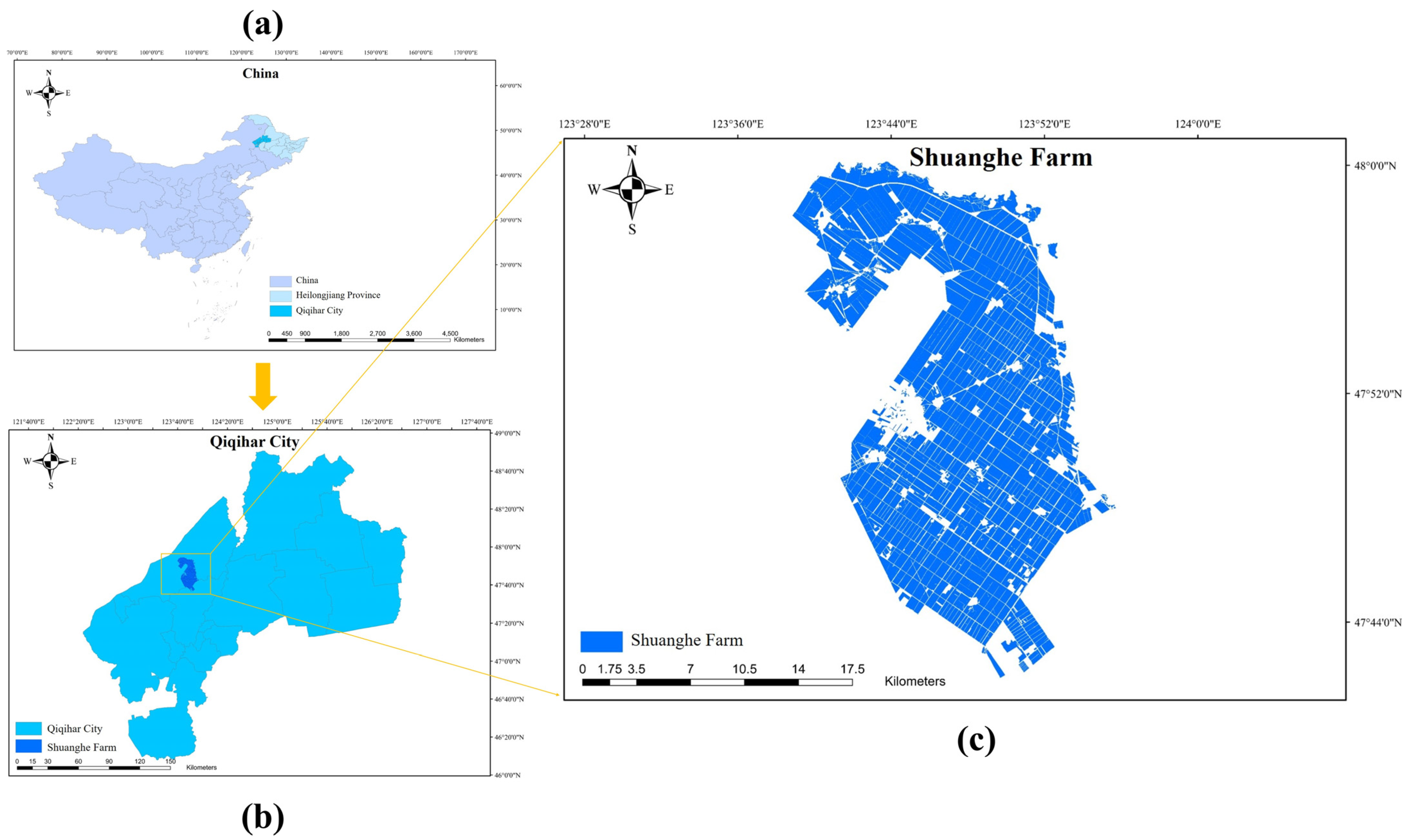
Shuanghe Farm (123°28′~124°00′E, 47°44′~48°00′N) is located in the mid-eastern part of Gannan County, Qiqihar City, Heilongjiang Province, along the western bank of the Arun River, at the junction of the southern slopes of the Greater Khingan Mountains and the Songnen Plain, bordering the Meilisi District of Qiqihar City (Figure 1). The total area of Shuanghe Farm is 38,000 hectares, with approximately 34,700 hectares in Gannan County and 2700 hectares in Meilisi. The region experiences a cold temperate continental monsoon climate, with distinct seasons. The average annual temperature is 2.6 °C, with a maximum of 39.2 °C and a minimum of −35.4 °C. There are 139 days with daily average temperatures above 10 °C, with a total accumulated temperature of 2562.9 °C. The average annual precipitation is 455.2 mm. Shuanghe Farm is primarily operated through large-scale mechanized farming and features flat terrain, contiguous land, well-organized plots, fertile soil, abundant sunlight, and rich water resources. The main crops grown are corn and rice, with additional crops including soybeans, miscellaneous grains (e.g., mung beans, black beans, red beans), and vegetables. The farm also has scattered woodlands, grasslands, and reed wetlands along its eastern boundary, with related buildings and facilities. The growing season for the main crops—corn, rice, and other crops—lasts from April to October [35,36].
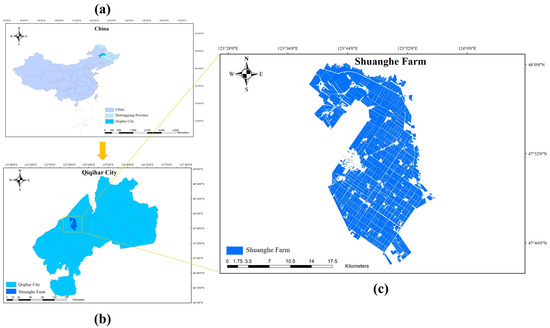
Figure 1.
(a) Heilongjiang Province, China; (b) Qiqihar City, Heilongjiang Province; (c) farmland-scale cultivated land quality study area in the black soil region.
2.2. Farm-Scale Cultivated Land Quality Dataset
We obtained a cultivated land quality dataset and the corresponding distribution vector map for Shuanghe Farm in 2022. The dataset contains a total of 1745 data entries, derived from soil samples collected and analyzed in a laboratory. The calculation method for cultivated land quality follows the guidelines in the Quality Grades of Cultivated Land (GB/T 33469-2016 [37]). The final classification divides the cultivated land quality into six grades, where the lower the grade number, the higher the cultivated land quality. In the 2022 dataset for Shuanghe Farm, Grade 1 represents the best land quality, while Grade 6 indicates the poorest. In the cultivated land quality distribution vector map, the land quality is displayed by vector map units, with each vector block representing a specific plot of land, and each plot is assigned a quality grade. The vector map of Shuanghe Farm is shown in Figure 1c.
2.3. Satellite Image Data and Preprocessing
Landsat 9, launched in September 2021 as part of the joint NASA-USGS Landsat program, carries two primary remote sensing instruments: the Operational Land Imager 2 (OLI-2) and the Thermal Infrared Sensor 2 (TIRS-2). The OLI-2 sensor captures data across nine spectral bands, including visible (coastal aerosol: 0.43–0.45 μm, blue: 0.45–0.51 μm, green: 0.53–0.59 μm, red: 0.64–0.67 μm), near-infrared (0.85–0.88 μm), shortwave infrared (SWIR1: 1.57–1.65 μm, SWIR2: 2.11–2.29 μm), panchromatic (0.50–0.68 μm), and cirrus (1.36–1.38 μm) wavelengths, with a spatial resolution of 30 m for multispectral bands and 15 m for the panchromatic band. The TIRS-2 instrument operates in two thermal infrared bands (10.6–11.19 μm and 11.50–12.51 μm) with a spatial resolution of 100 m, resampled to 30 m to match the multispectral data. This sensor configuration enables comprehensive land surface monitoring with improved radiometric performance and signal-to-noise ratios compared to previous Landsat missions, facilitating enhanced capabilities for environmental monitoring, agricultural assessment, and climate change research applications.
The Landsat 9 OLI-2/TIRS-2 satellite remote sensing images used in this study were sourced from the Landsat 9 Surface Reflectance Tier 2 dataset in GEE. All surface reflectance data in this dataset underwent atmospheric correction. The remote sensing images include five visible and near-infrared (VNIR) bands, as well as two shortwave infrared (SWIR) bands, which were orthorectified to obtain surface reflectance data. Additionally, one thermal infrared (TIR) band was orthorectified to obtain surface temperature data. Additionally, this dataset includes intermediate bands used for calculating Surface Temperature (ST) products, as well as Quality Assurance (QA) band data. Based on this image dataset, the study used GEE combined with machine learning algorithms to select remote sensing images of 4 typical periods from a total of 66 Landsat 9 images taken between January and December 2022, which were suitable for evaluating the cultivated land quality of Shuanghe Farm. The specific selection process was as follows. First, remote sensing images of the target area were cropped using the vector map of Shuanghe Farm. Then, pixel sampling of the remote sensing images was conducted based on the cultivated land quality distribution vector map of Shuanghe Farm. Due to the limitations of the GEE platform, the sampling resolution could not be set too small. Therefore, in this study, the sampling resolution was set to 290, allowing for the extraction of sampled pixels and the corresponding cultivated land grade values for the target area. Finally, we established a random forest classification model on the GEE platform. This model was based on the SR1 to SR7 band data of the sampled pixels in the target area and the cultivated land quality grade data. As a result, the model produced performance prediction data for the cultivated land quality grades for all Landsat 9 remote sensing images of Shuanghe Farm in 2022. Data with significant cloud cover or missing areas were excluded, and 21 remote sensing images from different periods were selected. These images were used for cultivated land quality evaluation using the random forest classification model in GEE. The model’s performance was assessed by the classification accuracy of Grades 1 to 6, overall accuracy, and the Kappa coefficient. The remote sensing images corresponding to the highest classification accuracy, overall accuracy, and Kappa coefficient for each grade were selected as the remote sensing images of typical periods suitable for evaluating cultivated land quality at Shuanghe Farm. Ultimately, remote sensing images of four typical periods were selected, as detailed in Table 1.

Table 1.
Remote sensing images of typical periods suitable for evaluating cultivated land quality at Shuanghe Farm.
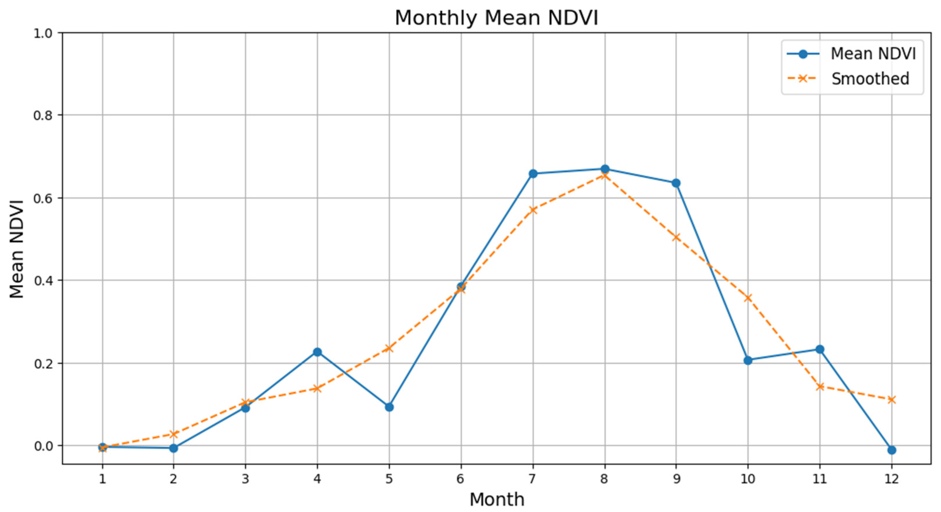
A foundational step in our proposed deep learning framework is the selection of optimal temporal windows from which to extract raw spectral reflectance data. Rather than using the entire time-series, which can introduce noise and computational inefficiency, we employed a Random Forest (RF) model within the Google Earth Engine (GEE) platform to identify the months yielding the highest classification performance. This data-driven approach pinpointed April, May, August, and October as the most informative periods. The high accuracy achieved by the RF model in these months indicates that they contain the most distinct spectral signatures for differentiating cultivated land quality classes.
The selection of April and August corresponds to the critical phenological stages of green-up and peak maturity, respectively. According to Figure 2 of monthly mean NDVI curve, April marks the onset of the growing season. During this green-up phase, the landscape is a heterogeneous mixture of bare black soil and emerging seedlings. This creates strong contrasts in the raw spectral reflectance across multiple bands, providing unique signatures that are crucial for the model to distinguish different early-season growth patterns. Conversely, August represents the period of maximum canopy density and photosynthetic activity, as indicated by the peak mean NDVI. At this stage, the pure and stable spectral signal from the dense vegetation canopy, with minimal soil background influence, serves as a key proxy for land quality.
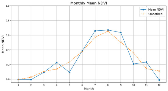
Figure 2.
Monthly mean NDVI curve.
The transitional months of May and October were identified as essential for capturing the dynamic phases of rapid growth and senescence. In May, crops are in a state of rapid development, leading to a swift increase in biomass and changes in canopy structure. The variability in spectral reflectance during this month reflects the diverse growth rates among different plots, offering critical information for classification. October captures the senescence phase, where a decline in chlorophyll and moisture content causes a significant shift in spectral reflectance. This period is also characterized by post-harvest bare soil for some early-maturing crops, further increasing the spectral heterogeneity across the farm.
2.4. Selecting Satellite-Derived Indicators for CLQ Evaluation
Since the four typical periods remote sensing images selected through the GEE random forest classification model (Table 1) had already undergone atmospheric and radiometric correction within the GEE platform, the Python 3.4.3 rasterio package was used to read the remote sensing image files, and geopandas package was used to read the vector files of Shuanghe Farm. Subsequently, the reflectance data for all bands of the remote sensing images were extracted using each plot within the farm area as the basic unit. The specific extraction method involved extracting the reflectance data for all pixels within a vector plot unit. The quartile method was then used to remove any outlier pixel band data from these values. The quartile method is a statistical technique used to describe the distribution of a dataset. When the reflectance dataset within a plot unit is ordered from smallest to largest, it is divided into four equal parts, each containing 25% of the data. These four segments are the first quartile (Q1), median (Q2), third quartile (Q3), and fourth quartile (Q4), respectively. The first quartile is the 25th percentile of the dataset, separating the lowest 25% from the remaining 75%. The third quartile is the 75th percentile of the dataset, separating the lowest 75% from the remaining 25% [38]. This study uses the difference between the third quartile (Q3) and the first quartile (Q1), with the purpose of excluding the top and bottom 25% of the data, retaining only the middle 50% of the dataset. Afterward, the average reflectance value of all remaining pixels is calculated, providing the complete band reflectance data for the vector plot unit. This method is applied to all plot units within the farm area, resulting in a total of 1413 Landsat 9 full-band reflectance datasets based on the individual plot units.
In this study, the reflectance of the seven spectral bands from Landsat 9 remote sensing, extracted using the method described above, is directly used as input for the cultivated land quality assessment model at the farm scale. Additionally, to facilitate comparison with other studies, based on the extracted spectral reflectance of the seven bands from Landsat 9, the study also calculates five commonly used vegetation indices in cultivated land quality evaluation: NDVI, EVI, SAVI, RVI, and DVI [17,19,39]. This allows for a subsequent comparison between the farm-scale cultivated land quality assessment model based directly on spectral band data and the model based on vegetation indices. All the indicators used in the farm-scale cultivated land quality assessment based on Landsat 9 satellite remote sensing in this study are shown in Table 2.
Table 2.
Indicators for field-scale cultivated land quality assessment based on Landsat 9 satellite remote sensing.
2.5. The Proposed BO-Stacking-TabNet Model
The BO-Stacking-TabNet Model is an enhanced deep learning architecture that integrates Bayesian Optimization (BO) with Stacking ensemble learning into the original TabNet framework for improved tabular data classification. The model employs a two-tier hierarchical structure consisting of base learners and a meta-learner, both utilizing TabNet encoders with optimized hyperparameters determined through Bayesian Optimization.
2.5.1. Feature Transformer Module
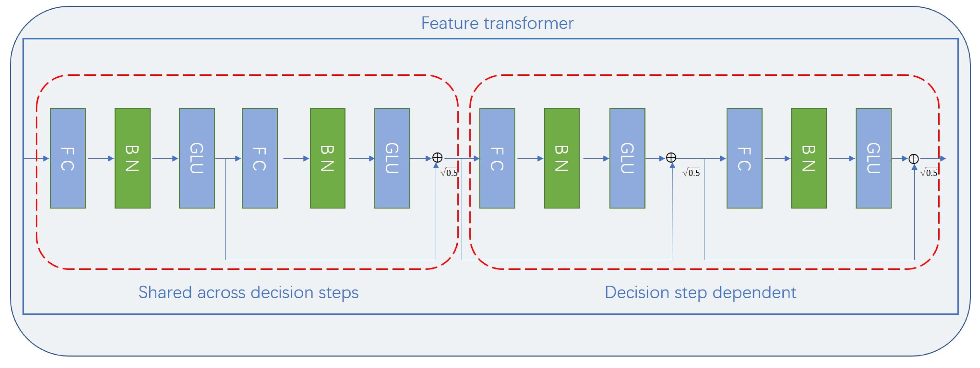
The Feature Transformer is one of the core modules of TabNet. Its primary goal is to extract high-dimensional feature representations from the input data. Through a series of linear transformations, nonlinear activations, residual connections, and dynamic feature selection mechanisms, it maps the input features into a high-dimensional latent space, while ensuring training stability and model interpretability.
From an architectural perspective, the structure of the Feature Transformer module enables efficient feature representation learning and step-by-step decision making through two parts working in synergy: the shared part (Shared across decision steps) and the decision step-dependent part (Decision step dependent). The design of these two parts is key to TabNet’s ability to progressively extract higher-order features, perform sparse feature selection, and maintain modularity and efficiency [45,46]. The overall architecture of the Feature Transformer is shown in Figure 3.
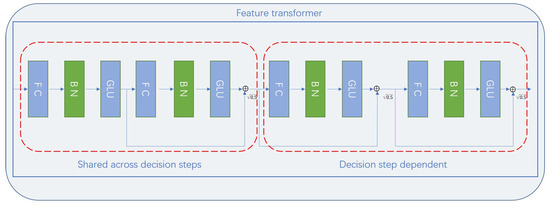
Figure 3.
Module structure of the Feature Transformer.
2.5.2. Attentive Transformer Module
The Attentive Transformer is one of the core components of the TabNet model. Its primary function is to perform dynamic feature selection through the attention mechanism, thereby selecting the most relevant subset of features at each decision step based on the input data.
The primary task of the Attentive Transformer is to select the most important subset of features at each decision step, thereby efficiently utilizing the input features in the multi-step decision process of TabNet. This enhances the model’s feature selection capability, significantly improves inference efficiency in high-dimensional data scenarios, effectively selects a small number of features, reduces redundant computations, enhances the model’s interpretability, and improves the model’s generalization ability. The specific structure of the Attentive Transformer module is shown in Figure 4.
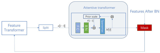
Figure 4.
Module structure of the Attentive Transformer.
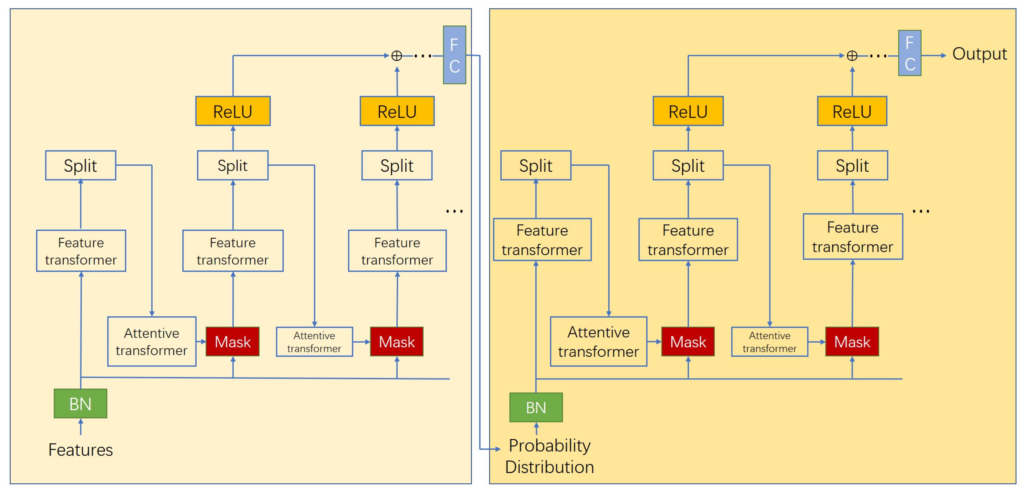
2.5.3. Stacking-Encoder Architecture
This study builds upon the TabNet model and integrates the idea of Stacking ensemble learning to improve the Encoder architecture, thereby further enhancing the performance of the TabNet model. Additionally, the Bayesian optimization algorithm is used to optimize the hyperparameters of both the base learners and the meta-learner [47]. Stacking is a technique that improves prediction performance by combining multiple different models. The core idea is to employ a two-layer model consisting of base learners and a meta-learner to achieve a hierarchical structure. The outputs of multiple models are used as new inputs to construct a model with improved performance. Figure 5 illustrates the overall architecture of the Stacking-Encoder in the BO-Stacking-TabNet model. In this architecture, the BO-Stacking-TabNet model is composed of two Encoder structures with similar architecture but different hyperparameters, serving as the base learners and meta-learner in the Stacking structure. These two Encoder architectures are optimized for hyperparameters using the Bayesian optimization algorithm prior to training, ensuring that the model achieves optimal training performance.
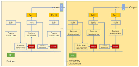
Figure 5.
Overall architecture of the Stacking-Encoder.
Regarding the Encoder architecture, the original numerical features are fed directly into the model without any global feature normalization, and only batch normalization (BN) is applied to the input features. The same--dimensional original input features are passed to each decision step of the base learner Encoder. The category probability distribution output by the base learner Encoder serves as the input features for the meta-learner Encoder , where represents the batch size and represents the number of categories. The encoding process in TabNet is based on sequential multi-step processing, where information processed in step is used as input for step , to determine which features to use and output the processed feature representations, which are then aggregated into the overall decision.
The data processing flow of the Stacking-Encoder is roughly divided into two stages: feature selection and feature processing. In the feature selection stage, the model sets learnable masks to perform soft selection of significant features. The base learner Encoder mask is denoted as , and the meta-learner Encoder mask is denoted as . By sparsely selecting the most significant features, the learning capacity of the decision steps is not wasted on irrelevant features, thus improving the parameter efficiency of the model. The mask is multiplicative , and at the same time, an attentive transformer is used to obtain the mask based on the features processed in the previous step, i.e., .
Moreover, is the prior scale term, which represents how many specific features were previously used, i.e., , where is the relaxation parameter. When all values are initialized to 1, that is, or , there is no prior on the masked features. Additionally, the model uses sparsity regularization to further control the sparsity of the selected features, i.e., or , where is a numerical stability factor. The sparsity regularization is then added to the overall loss function, weighted by a sparsity coefficient .
In terms of feature processing, the TabNet model uses a feature transformer to process the filtered features, which are then split into two parts. One part is used for the output of the decision steps, while the other part provides information for subsequent processing steps, i.e., , where and , as shown in Figure 3.
Finally, based on the decision manifold idea of class decision trees, the overall decision embedding of the TabNet model is , which is then applied to a linear mapping to obtain the output mapping. For the base learner Encoder, the output mapping is the category probability distribution, while for the meta-learner Encoder, based on the category probability distribution input, the output mapping is the final predicted category data.
The following Table 3 summarizes the key hyperparameter configurations for the entire training process. Explicit data normalization was not performed. The data was fed directly into the model for training, as the TabNet architecture incorporates internal batch normalization layers that provide an intrinsic normalization mechanism.
Table 3.
Model training configuration.
2.6. Modeling Evaluation
For classification problems, evaluating the model’s classification performance is crucial. Currently, we mainly use four metrics—, , , and —in combination to comprehensively assess the model’s classification performance [48]. Therefore, this study selected , , , and as the four metrics to quantitatively evaluate the model’s effectiveness. For this study, the formula for calculating accuracy is as follows:
where represents the number of positive samples correctly classified as positive, represents the number of negative samples correctly classified as negative, represents the number of negative samples incorrectly classified as positive, and represents the number of positive samples incorrectly classified as negative.
In this study, the macro-average method is used to aggregate the performance results of different metrics across all classes. Specifically, this method averages the evaluation metrics (such as , , ) by summing them for each class and then dividing by the number of classes. This approach gives equal weight to all classes, treating each class equally. It also fully considers rare classes with small proportions in the dataset [49].
For the farm-scale cultivated land quality grade dataset, there is a significant disparity in the distribution of different land quality grades. High-grade and low-grade cultivated land often accounts for only a small proportion of the data, yet these grades are precisely the ones that are of particular interest in the study, holding significant practical relevance. Therefore, the macro-average method is highly suitable for such imbalanced class distributions.
3. Results
3.1. Model Performance Evaluation Based on Typical Vegetation Indices
We utilized the spectral reflectance of seven bands from Landsat 9 remote sensing images extracted for four typical periods, and five commonly used vegetation indices for cultivated land quality assessment were selected, namely NDVI, EVI, SAVI, RVI, and DVI. The calculation formulas for these indices are provided in Table 2. The data from the four periods—April, May, August, and October 2022—were used to calculate the five vegetation indices, resulting in a total of 20 model input variables, which served as the input for our model. We compared the performance of our proposed BO-Stacking-TabNet model against other commonly used machine learning models in the field of remote sensing-based cultivated land quality assessment. All models were optimized using Bayesian optimization to achieve the best hyperparameters. Table 4 presents the final performance results. As seen in Table 4, the BO-Stacking-TabNet model outperformed all others in terms of Accuracy, Precision, Recall, and F1 score. The original TabNet model, without any improvements, also demonstrated strong performance, ranking second in terms of Accuracy, Recall, and F1 score. The Random Forest model showed excellent performance in Precision, ranking second in that category, and its Accuracy was relatively good. However, its performance was mediocre in terms of Recall and F1 score. XGBoost exhibited relatively good and stable performance across Accuracy, Precision, Recall, and F1 score. CatBoost, although slightly inferior to XGBoost in these four metrics, still showed relatively strong performance. LightGBM, on the other hand, only performed well in terms of Accuracy, ranking poorly in the other three metrics. Gradient Boosting Trees (GBT) performed well in Accuracy, slightly better than Random Forest, but had average performance in the other three metrics. Overall, only the TabNet and BO-Stacking-TabNet models showed consistently superior performance across all metrics, which demonstrates TabNet’s excellent capabilities in the evaluation of cultivated land quality based on vegetation indices. Additionally, the BO-Stacking-TabNet model enhanced the original TabNet model’s performance, with an increase in Accuracy by 0.7%, Precision by 19.6%, Recall by 0.03%, and F1 score by 1.16%. This confirms the effectiveness of our improved BO-Stacking-TabNet model in enhancing the performance of the TabNet model.
Table 4.
Model performance evaluation based on typical vegetation indices as input variables.
3.2. Model Performance Evaluation Based on Spectral Reflectance
We used the spectral reflectance data from seven bands of Landsat 9 remote sensing images collected during four typical periods in 2022, namely April, May, August, and October. Without applying any band filtering, a total of 28 indicators were directly used as model inputs, with the spectral reflectance information for these seven bands presented in Table 2. The BO-Stacking-TabNet model, which was proposed in this study, was compared with other commonly used machine learning models in the field of remote sensing-based cultivated land quality assessment. All models were optimized using Bayesian optimization to achieve their optimal hyperparameters. The performance results of these models are displayed in Table 5. As shown in Table 5, the BO-Stacking-TabNet model achieved the best performance across all four metrics: Accuracy, Precision, Recall, and F1 score. The original, unmodified TabNet model also performed exceptionally well, ranking second in Accuracy, Recall, and F1 score. Outside of the TabNet and BO-Stacking-TabNet models, the Random Forest model showed strong performance in Precision, ranking second in this category. However, its performance in Accuracy, Recall, and F1 was relatively mediocre. The XGBoost model demonstrated stable performance across all four metrics (Accuracy, Precision, Recall, and F1 score). CatBoost performed similarly to XGBoost in terms of Accuracy and Precision but performed better than XGBoost in Recall and F1, showcasing good overall performance. In contrast, LightGBM had the weakest performance across all four metrics. Gradient Boosting Trees (GBT) performed well overall, showing better results than CatBoost in terms of Accuracy, Precision, Recall, and F1 score, albeit by a small margin. Overall, the BO-Stacking-TabNet model exhibited superior, comprehensive performance, while the original TabNet model also stood out, further validating the effectiveness of the improvements made in the BO-Stacking-TabNet model.
Table 5.
Model performance evaluation based on spectral reflectance as input variables.
Therefore, from the above analysis, it can be concluded that only the TabNet model and BO-Stacking-TabNet model demonstrated consistently outstanding performance across all metrics. This confirms that the TabNet model also performs excellently in evaluating cultivated land quality based on spectral reflectance. Moreover, the BO-Stacking-TabNet model improved upon the TabNet model, with increases of 2.13% in Accuracy, 12.59% in Precision, 1.83% in Recall, and 2.19% in F1 score. These improvements clearly demonstrate the effectiveness of the enhancements made to the TabNet model in the BO-Stacking-TabNet. Additionally, as seen in Table 5, models using spectral reflectance as input variables showed significant improvements in Accuracy, Precision, Recall, and F1 score compared to models using vegetation indices as input. Specifically, the BO-Stacking-TabNet model using spectral reflectance achieved an increase of 10.62% in Accuracy, 1.55% in Precision, 11.05% in Recall, and 10.18% in F1 score compared to the BO-Stacking-TabNet model using vegetation indices as input. This significantly demonstrates the reliability of using Landsat 9 spectral reflectance for farmland-scale cultivated land quality assessment.
Meanwhile, since Cultivated Land Quality (CLQ) is an ordinal variable for which traditional classification methods may not be optimal, we introduced two ordinal classification models: Ordinal Logistic Regression and the CORAL neural network. The results indicate that the Cordinal classification models achieves a slight improvement in overall performance across most metrics compared to the traditional classification methods. Although the CORAL neural network shows strong precision (0.6831), our BO-Stacking-TabNet surpasses it not only in precision but also in recall and overall accuracy. This suggests that while modeling the ordinal nature of CLQ is beneficial, the advanced feature representation and optimization strategies in our proposed model allow it to capture more complex underlying patterns, leading to more accurate predictions.
3.3. Comparative Analysis with Deep Learning Approaches
To accurately evaluate the performance of BO-Stacking-TabNet, we conducted a comprehensive comparative analysis against several prevalent deep learning architectures commonly used in precision agriculture. The models selected for comparison include CNN-RNN hybrid models, a standard Transformer-based regressor, and a ResNet-LSTM hybrid. All models were trained for 300 epochs on the same dataset to ensure a fair and direct comparison. The performance metrics, including Accuracy, Mean Squared Error (MSE), Root Mean Squared Error (RMSE), Mean Absolute Error (MAE), and the coefficient of determination (R2), are presented in Table 6.
Table 6.
Comparative experimental results for deep learning approaches.
The results clearly demonstrate the superior performance of our proposed model, BO-Stacking-TabNet. With an accuracy of 72.41%, our model significantly outperforms the ResNet-LSTM hybrid (68.60%), the Transformer Regressor (70.18%), and the CNN-RNN hybrid models (69.01%). This notable increase in accuracy underscores the effectiveness of our model’s unique architecture in capturing the complex patterns and dependencies within the agricultural dataset.
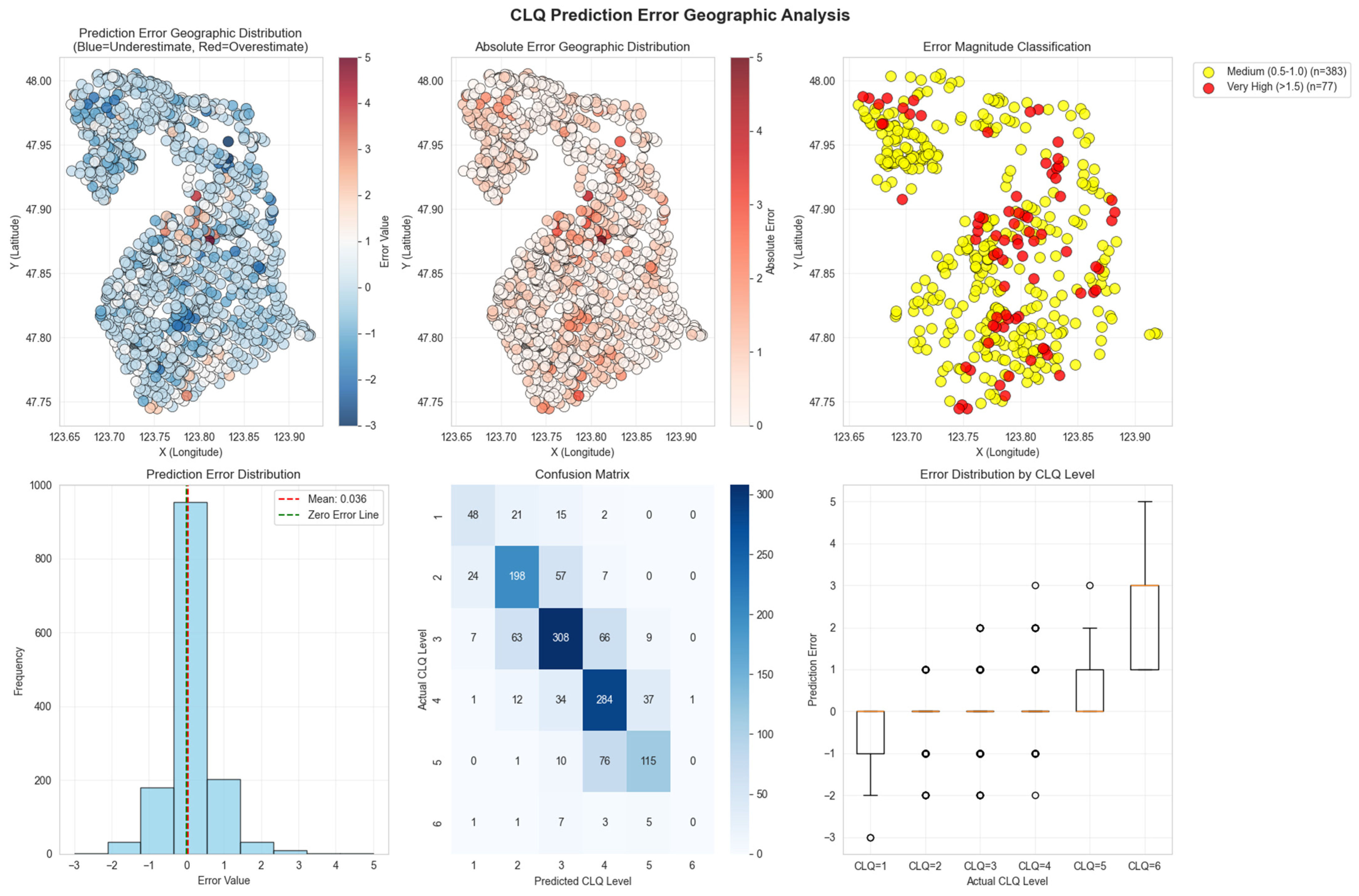
3.4. Confusion Matrix and Spatial Analysis
To conduct a comprehensive error analysis as suggested, we further dissected the model’s performance by examining the confusion matrix, per-grade error distribution, and the spatial patterns of prediction errors.
A detailed breakdown of classification performance is presented in the confusion matrix (Figure 6, center-bottom). The matrix reveals that the model performs well, with high values along the diagonal, indicating a large number of correct classifications for all Cultivated Land Quality (CLQ) grades. The primary source of error stems from confusion between adjacent grades. For instance, for CLQ-3, seven parcels were misclassified as CLQ-2 and sixty-six were misclassified as CLQ-4. Similarly, for CLQ-4, 12 parcels were misclassified as CLQ-3 and 34 as CLQ-5. This pattern is logical, as adjacent grades possess more similar soil and environmental characteristics, making them harder to differentiate. Importantly, severe misclassifications across non-adjacent grades were rare, underscoring the model’s reliability.

Figure 6.
CLQ prediction error geographic analysis.
The per-grade error analysis (Figure 6, bottom-right) further clarifies this trend. The boxplot shows the distribution of prediction errors (Predicted Grade—Actual Grade) for each CLQ level. It is observed that the median error for all grades is close to zero, but the variance of the error (interquartile range) tends to increase with the CLQ grade. This suggests that while the model is generally unbiased for each class, its predictions for higher-quality land (e.g., CLQ-5 and CLQ-6) are subject to greater uncertainty and larger potential errors compared to lower-quality land.
The geographic distribution of prediction errors reveals distinct spatial patterns (Figure 6, top panel). The Error Magnitude Classification map (top-right) highlights that parcels with medium (0.5 < |error| ≤ 1.0, n = 383) and very high (|error| > 1.5, n = 77) absolute errors are not randomly distributed. Instead, they exhibit significant spatial clustering, particularly in the northern and central–eastern parts of the study area. This spatial aggregation of errors suggests that the model’s performance is influenced by local factors not fully captured by the input variables, which is likely attributable to intra-field heterogeneity. These regions might be characterized by more complex cropping patterns, varied irrigation, or sudden changes in soil type within single parcels, which can confound the spectral signals used for prediction.
To statistically validate this visual observation, we performed a spatial autocorrelation analysis on the prediction errors. The calculation yielded a Global Moran’s I statistic of 0.0270 (p < 0.01). This positive and statistically significant value confirms a moderate spatial autocorrelation in the prediction errors. This result provides quantitative evidence that the model’s errors are spatially dependent—that is, overestimated and underestimated parcels tend to cluster together—reinforcing the hypothesis that localized spatial processes and field heterogeneity affect the model’s accuracy.
3.5. Model Interpretability and Feature Importance
To investigate the basis of our model’s decisions, we adopted SHAP (Shapley Additive exPlanations) to conduct a feature importance analysis on the trained BO-Stacking-TabNet model. Unlike methods that rely on a model’s internal structure, SHAP is founded on cooperative game theory, providing a fair, consistent, and model-agnostic quantification of the marginal contribution of each feature to the final prediction. This approach serves as a generally accepted standard for explaining complex models.
The SHAP analysis result is shown as Figure 7, which revealed the key features that were most influential in classifying cultivated land quality. Among all input features, spectral data from August and October were identified as the most critical periods. Specifically, the B6 band from August (SR_08_B6), the B7 band from October (SR_10_B7), and the B1 band from April (SR_04_B1) exhibited the highest mean absolute SHAP values. This indicates they were the core drivers of the model’s decisions. The high importance of bands from August, corresponding to the peak crop growing season, and October, the post-harvest period, aligns well with established phenological principles for assessing land quality, as these periods provide vital information about vegetation health and exposed soil conditions, respectively.
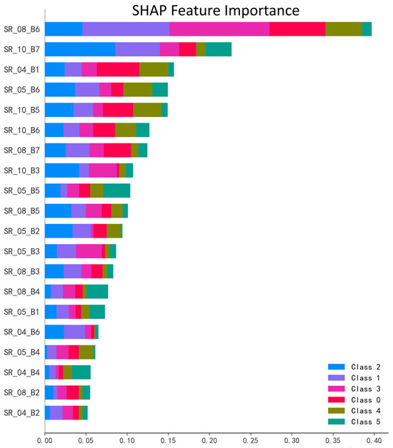
Figure 7.
Feature importance ranking of Landsat 9 spectral bands during typical periods based on the SHAP.
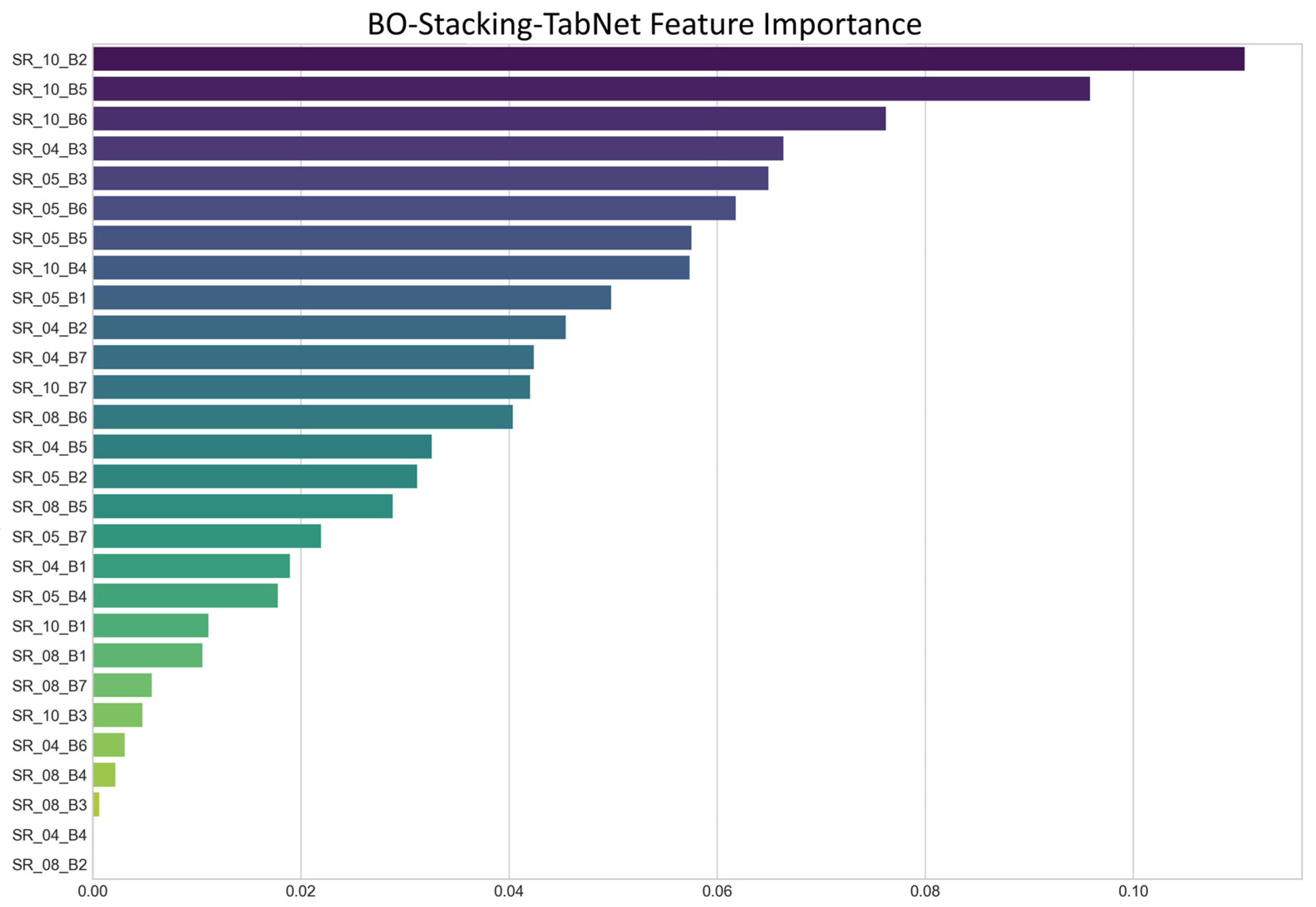
Beyond this global contribution analysis, we further explored TabNet’s native feature importance, which is derived from its internal attention masks, and the result is shown as Figure 8. The purpose of this second analysis is not to replace the SHAP results, but to gain a deeper insight into the internal working mechanism of our specific BO-Stacking-TabNet model. This importance measure reflects the model’s attention or how frequently it utilizes a feature across its sequential decision-making steps.

Figure 8.
Feature importance ranking of Landsat 9 spectral bands during typical periods based on the BO-Stacking-TabNet model.
A comparative analysis of the two methods provides a more profound understanding of the model’s behavior. We observed a strong consensus in the key predictive periods, with both SHAP and TabNet’s internal mechanism highlighting the significance of features from October and August. For instance, the B5 band from October (SR_10_5) ranks highly in both analyses. This consistency across two distinct methodologies provides strong, cross-validated evidence for the critical role of these features.
More interestingly, the comparison reveals the unique architectural advantages of TabNet. Some features with high contribution scores in the SHAP analysis, for instance, the B3 band from October (SR_10_B3), were assigned relatively lower weights by TabNet’s attention mechanism. This is not a contradiction but rather a demonstration of TabNet’s efficiency and sparse feature selection. Through its sequential, multi-step decision process, the model learns to make predictions using sparse combinations of features. Once the model has extracted sufficient information from certain features in early decision steps, it may no longer need to heavily attend to other highly correlated or information-redundant features in subsequent steps.
3.6. Spatial Distribution and Regional Validation of Cultivated Land Quality
The 2022 dataset of cultivated land quality for Shuanghe Farm categorizes the quality of cultivated land into six grades, with Grade 1 being the highest and Grade 6 the lowest. The distribution of cultivated land quality is illustrated in Figure 9a. From Figure 9a, it can be observed that Grade 1 and Grade 2 lands are primarily located in the northeast and southwest regions of Shuanghe Farm. Grade 3 land is mainly distributed in the central and southeastern parts of the farm, with some presence in the northwest as well. Grade 4 and Grade 5 lands are concentrated on the western–central edge, the northwest, and the southeastern margins, with sporadic distributions in the central–southern area. Grade 6 land is mainly distributed in the central–western region. In terms of proportional distribution within the dataset, Grade 1 land accounts for 6.48%, Grade 2 for 19.54%, Grade 3 for 30.89%, Grade 4 for 29.00%, Grade 5 for 12.84%, and Grade 6 for 1.25%. Based on the distribution of different grades of cultivated land, it can be seen that Shuanghe Farm’s cultivated land is primarily composed of Grade 2, Grade 3, and Grade 4, with a significant proportion of Grade 5. Grade 1 and Grade 6 lands are less prevalent, with Grade 6 being the scarcest. Overall, the quality of cultivated land in Shuanghe Farm can be considered moderate, with the northeast and southwest regions having relatively higher-quality land, the central and southeastern regions possessing moderate quality, and the northwest showing poorer land quality.
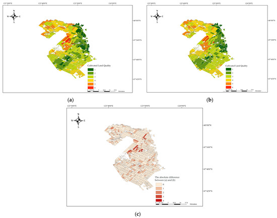
Figure 9.
(a) The 2022 distribution map of cultivated land quality in Shuanghe Farm; (b) predicted 2022 distribution map of cultivated land quality in Shuanghe Farm based on Landsat 9 remote sensing imagery and the BO-Stacking-TabNet model; (c) absolute difference between actual and predicted values of cultivated land quality.
The cultivated land quality evaluation results from the BO-Stacking-TabNet model, which uses spectral reflectance from Landsat 9 during typical periods as input indicators, are shown in Figure 9b. A comparison of Figure 9a,b reveals that the spatial distribution of cultivated land quality is largely consistent between the two. Based on the proportional distribution of land quality grades in the model’s evaluation results, Grade 1 accounts for 6.36%, Grade 2 for 19.31%, Grade 3 for 31.98%, Grade 4 for 28.54%, Grade 5 for 13.18%, and Grade 6 for 0.63%. When comparing these figures to the proportional distribution of cultivated land quality in the Shuanghe Farm dataset, the differences in the proportions for Grades 1, 2, 4, 5, and 6 are all less than 1%. In contrast, the difference for Grade 3 is slightly larger, but the two datasets differ by only 1.09%. Therefore, based on the proportional distribution, the BO-Stacking-TabNet model’s evaluation results, which use Landsat 9 spectral reflectance as input, are essentially consistent with the cultivated land quality dataset of Shuanghe Farm.
This study also calculated the absolute difference between the cultivated land quality evaluation grades from the Shuanghe Farm dataset and those obtained from the Landsat 9-based remote sensing model during typical periods. The distribution of these differences is shown in Figure 9c. From Figure 9c, it can be seen that the vast majority of the farm’s cultivated land has consistent evaluation grades between the two methods. In areas where discrepancies exist, fields with a difference of 1 or 2 grades are mainly located in the central–southern and northwestern regions of Shuanghe Farm, with sporadic distributions in the central–northern area. Fields with differences of 3 or 4 grades are primarily found in the central–northern region, with occasional distributions in the central–southern and northwestern parts of the farm. Statistically, 83.95% of the land shows consistent evaluation grades between the two methods. Fields with a difference of 1 grade account for 13.18%, those with a difference of 2 grades account for 2.06%, fields with a difference of 3 grades represent 0.52%, and those with a difference of 4 grades represent 0.29%. Therefore, the statistical data indicate that the cultivated land quality evaluation results based on the Landsat 9 remote sensing model are generally consistent with the evaluation results of Shuanghe Farm. Among the cases where the evaluation grades differ, the vast majority show a difference of only 1 grade, with differences of 2, 3, or 4 grades being relatively rare, further supporting the reliability of the model’s evaluation results.
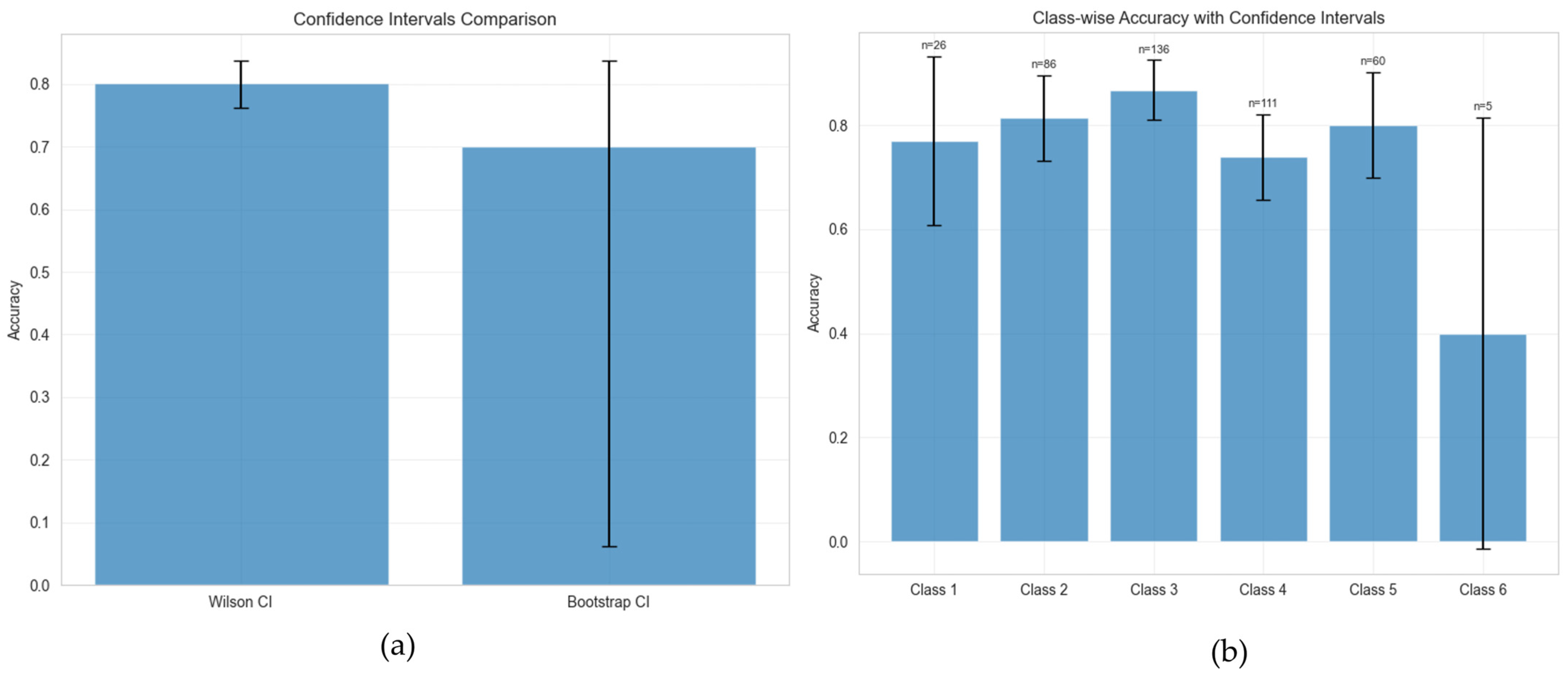
3.7. Dataset Uncertainty and Reliability Analysis
To rigorously evaluate the robustness and predictive reliability of the proposed model, a comprehensive uncertainty analysis was conducted. Beyond overall accuracy metrics, it is crucial to understand the model’s confidence in its predictions, both globally and for individual classes. This analysis was performed on the independent test set, which comprises 424 samples distributed across six distinct land quality classes.
We first assessed the confidence interval for the model’s overall accuracy using two standard methods: the Wilson Score Interval and the Bootstrap Confidence Interval. The results are presented in Figure 10a. The Wilson Score Interval, which is well-suited for binomial proportions like accuracy, indicates that the model achieves an overall accuracy of approximately 80.0% with a remarkably tight confidence interval. This suggests a high degree of stability and reliability in the model’s aggregate performance. In contrast, the Bootstrap CI, while centered at a lower accuracy of approximately 70.0%, displays a significantly wider range. The large variance in the bootstrap estimate underscores the potential for instability in resampling-based evaluations, reinforcing the conclusion that the model’s true accuracy is more reliably represented by the stable and high-performing Wilson Score.
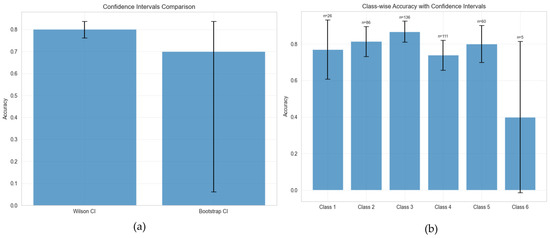
Figure 10.
(a) Confidence interval comparison; (b) class-wise accuracy with confidence intervals.
To gain deeper insight into the model’s behavior, we performed a class-wise accuracy analysis, with results and sample counts for each class shown in Figure 10b. This analysis reveals a strong correlation between predictive accuracy and the number of samples available for each class, highlighting the impact of the inherent data imbalance. The key findings showed that the model performs exceptionally well on classes with substantial representation, such as Class 3 (n = 136), Class 2 (n = 86), and Class 5 (n = 60), which achieved high accuracies (approx. 85%, 81%, and 80%, respectively) with narrow confidence intervals. For classes with moderate sample sizes like Class 1 (n = 26) and Class 4 (n = 111), the model maintained good performance (approx. 78% and 74%) with slightly wider confidence intervals, indicating reliable predictive capability. Conversely, the model’s primary limitation was exposed in the prediction of Class 6. With only n = 5 samples, its accuracy plummeted to approximately 40% with an extremely wide confidence interval, a result directly attributable to the scarcity of data.
4. Discussion
A scientific remote sensing-based method for evaluating cultivated land quality offers an efficient and quick way to understand the current status of land quality distribution, saving both labor and time. Remote sensing data has the advantages of wide coverage, easy accessibility, and rich information. Therefore, research on remote sensing-based evaluation of cultivated land quality has significant practical value. However, there is currently a lack of studies focusing on land quality evaluation at the farm scale, with most research in this area concentrating on larger scales. Our study, conducted in the black soil region of Shuanghe Farm in northeastern China, confirms the feasibility of applying remote sensing-based land quality evaluation at the farm scale. The regional validation of this study shows that the BO-Stacking-TabNet model, using Landsat 9 spectral reflectance from typical periods, produces classification results that are highly consistent with the spatial distribution and grade statistics of Shuanghe Farm’s cultivated land quality dataset. This indicates that the method for evaluating cultivated land quality based on Landsat 9 spectral reflectance is both reasonable and feasible.
Selecting the optimal remote sensing imagery period is a critical prerequisite for accurately evaluating cultivated land quality. The national standard ‘Quality Grades of Cultivated Land’ (GB/T 33469-2016) primarily bases its evaluation on intrinsic soil properties (e.g., physical, chemical, and nutrient characteristics) and topographical features. Consequently, imagery from bare-soil periods, when soil is maximally exposed, is traditionally considered ideal. However, rather than relying solely on this empirical assumption, this study implemented a systematic, data-driven experiment to quantitatively assess the performance of imagery from different key phenological periods. Our objective was to identify the most informative periods and understand the underlying reasons for their effectiveness.
We selected imagery from April/May (post-thaw and pre-sowing), August (peak growing season), and October (post-harvest). The strong performance of models using imagery from April, May, and October (as shown in Table 5) aligns with the traditional approach. During these bare-soil or semi-bare-soil periods, spectral information from the Landsat 9 sensor can directly capture variations in soil organic matter, moisture, and texture, providing a direct assessment of the soil background. A particularly noteworthy finding is the high classification accuracy achieved using imagery from August, the period of maximum vegetation cover. While vegetation can obscure the direct soil signal, it also functions as a highly effective bio-indicator of underlying soil quality. The health, density, and vigor of the crop are integrated expressions of the soil’s ability to provide water and nutrients. Our model successfully learned the complex relationship between the crop’s spectral characteristics during its peak growth and the intrinsic quality grade of the soil it grows in. This demonstrates that the crop’s phenotype serves as a robust proxy for the comprehensive land quality defined by the standard. This finding suggests that while bare-soil imagery reflects the static potential of the land, peak-season imagery captures its realized productive performance, offering a complementary and equally valuable perspective for evaluation. Therefore, our results provide a validated and more flexible set of temporal windows for remote sensing-based cultivated land quality assessment in the black soil region of Northeast China. Meanwhile, we acknowledge that our approach prioritizes classification accuracy over temporal representativeness, which may introduce temporal bias.
Traditionally, many studies have used vegetation index indicators derived from the spectral reflectance of remote sensing imagery as input for model evaluations. However, based on our research and the comparison shown in Table 4 and Table 5, it is evident that while models using vegetation indices as input perform well in cultivated land quality evaluation, models using spectral reflectance as input perform significantly better. All models using spectral reflectance as input show noticeable improvements compared to those using vegetation indices, demonstrating the feasibility and effectiveness of using spectral reflectance for land quality evaluation at the field scale. Models based on spectral reflectance as input can bypass certain steps, such as the selection of characteristic bands or the calculation of vegetation indices, and directly evaluate cultivated land quality based on the spectral reflectance from remote sensing imagery. This greatly simplifies the process of remote sensing-based land quality evaluation. However, whether this direct spectral reflectance-based evaluation method is applicable to farm scales outside the northeastern black soil region remains to be further explored and studied.
Our analysis of feature importance, presented in Figure 7 and Figure 8, provides strong evidence for the model’s robust learning mechanism. The findings revealed that spectral bands from August (peak growing season) and October (post-harvest bare soil) were most critical for the model’s predictions. This quantitatively validates our data-driven selection of temporal windows and aligns with established agronomic principles, where crop physiological status and exposed soil conditions serve as powerful proxies for underlying land quality. The fact that the model independently identified these phenologically significant periods, without prior manual feature engineering, significantly strengthens the confidence in our proposed method. Furthermore, the comparison between the model-agnostic SHAP analysis and TabNet’s internal attention mechanism highlighted the model’s efficiency in utilizing a sparse feature set. This confirms that the BO-Stacking-TabNet architecture not only achieves high accuracy but also develops an interpretable and efficient decision-making process, which is a key advantage for practical applications.
While this study successfully constructed a cropland quality evaluation model at Shuanghe Farm, we acknowledge its limitations, the most significant being the single-site nature of the research area. Due to the difficulty in obtaining validation data from other comparable regions, the model’s generalization capability across broader geographical ranges has not been sufficiently verified. However, this limitation also charts a clear course for our future research directions. Our immediate plan is to apply the existing model directly to other farms in the Northeast Black Soil Belt to assess its zero-shot transfer capability and to conduct an in-depth analysis of the key factors causing performance degradation. To address the issue of model portability, we will further explore more advanced machine learning techniques. For instance, introducing Domain Adaptation methods, particularly through Adversarial Training strategies, and using a small amount of unlabeled or labeled data from a target region to fine-tune the model, could enable it to rapidly adapt to the data feature distributions of the new area. Furthermore, for regions with sparse data, Few-shot Learning technology also offers a highly promising solution for the rapid development of localized models. In the long term, this research lays the methodological foundation for establishing a long-term dynamic monitoring system for cropland quality. Our ultimate goal is to integrate multi-year remote sensing imagery and ground observation data to explore the model’s temporal generalization capabilities, thereby making the critical leap from static evaluation to dynamic monitoring. Such a dynamic monitoring system will be able to provide more timely and robust decision-making support for the sustainable use and protection of black soil.
A detailed examination of the model’s class-wise accuracy (Figure 10b) points to a significant challenge stemming from the dataset itself; the model struggles with underrepresented classes, particularly CLQ-6. This issue stems directly from the inherent data imbalance and the scarcity of training samples for certain grades. To overcome this limitation and enhance the model’s generalization capability, our future work will focus on implementing advanced data augmentation techniques. Due to the very small number of samples for CLQ-1 and CLQ-6, using traditional augmentation methods like SMOTE would lead to severe overfitting. Therefore, some current research introduces potential data augmentation strategies, particularly for addressing spectral imbalances. For instance, Rana & Gatti [50] in their work on Comparative Evaluation of Modified Wasserstein GAN-GP and State-of-the-Art GAN Models for Synthesizing Agricultural Weed Images in RGB and Infrared Domain introduced the concept of using spectrally consistent, structurally coherent synthetic imagery, which is directly applicable to reflectance-based land classification. Furthermore, Cultivated Land Quality (CLQ) grades are inherently ordinal variables, where the penalty for misclassifying an adjacent class should be less than for a distant one. Although previous CLQ assessments have often employed multi-class classifiers, the experimental results in Table 5 indicate that ordinal classification models generally outperform traditional multi-class classifiers, which demonstrates the potential of these models in the field of CLQ assessment. In the future, we will investigate methods such as CORAL neural networks or ordinal regression with deep ensembles to more accurately model how land quality degrades over time.
5. Conclusions
This study utilized the GEE to select Landsat 9 satellite remote sensing images from the entire year of 2022 for evaluating cultivated land quality. The spectral reflectance of all bands from the selected Landsat 9 remote sensing images during typical periods was used as feature indicators for model input. An improved BO-Stacking-TabNet model was then employed to assess cultivated land quality at the farm scale in the black soil region of Northeast China. The main conclusions are as follows:
(1) Among the 66 Landsat 9 satellite remote sensing images analyzed in 2022, those from April, May, August, and October demonstrated the highest classification performance for evaluating cultivated land quality at the farm scale in the black soil region of Northeast China. This study established a preliminary farm-scale cultivated land quality assessment model using the random forest classification model on the GEE platform driven by classification metrics. By sequentially inputting all Landsat 9 remote sensing images from the entire year of 2022 into the model, the cultivated land quality assessment results were calculated and validated. The final results showed that the classification accuracy, overall accuracy, and Kappa values for the six land quality grades corresponding to the model results from the images in April, May, August, and October were the highest among all tested periods.
(2) In the remote sensing-based cultivated land quality assessment model at the farm scale in the black soil region of Northeast China, the model using spectral reflectance as input indicators comprehensively outperformed the model using vegetation indices as input indicators. Specifically, the BO-Stacking-TabNet model based on spectral reflectance as input indicators showed a 10.62% improvement in Accuracy, a 1.55% improvement in Precision, an 11.05% improvement in Recall, and a 10.18% improvement in F1-score compared to the BO-Stacking-TabNet model based on vegetation indices as input indicators.
(3) The BO-Stacking-TabNet model proposed in this study showed significant improvements in performance for cultivated land quality assessment compared to the original TabNet model. Using spectral reflectance as the input indicators for both models, the BO-Stacking-TabNet model demonstrated a 2.13% improvement in Accuracy, a 12.59% improvement in Precision, a 1.83% improvement in Recall, and a 2.19% improvement in F1-score over the TabNet model.
(4) The cultivated land quality assessment results of the BO-Stacking-TabNet model proposed in this study are accurate and reliable. Specifically, compared with the 2022 Shuanghe Farm cultivated land quality dataset, the results of the BO-Stacking-TabNet model showed that 83.95% of the assessment grades were consistent with the dataset, 13.18% differed by one grade, 2.06% differed by two grades, 0.52% differed by three grades, and 0.29% differed by four grades. The results of the BO-Stacking-TabNet model are generally consistent with the 2022 Shuanghe Farm cultivated land quality dataset.
We proposed an effective method for assessing cultivated land quality at the farm scale in the black soil region of Northeast China. By combining Landsat 9 satellite remote sensing images with the BO-Stacking-TabNet model, it provides a scientific basis for obtaining rapid, accurate, and convenient data on cultivated land quality at the farm scale, thereby guiding agricultural production and management.
Author Contributions
M.G.: Conceptualization, Formal analysis, Supervision, and Project administration; Z.Y. Methodology, Data curation, Investigation, Validation, and Original draft; X.L.: Formal analysis, Methodology, Original draft preparation and Funding acquisition; H.S.: Supervision and Validation; Y.H.: Review and Editing; B.Y.: Visualization; Y.Z.: Resources. All authors have read and agreed to the published version of the manuscript.
Funding
This research was funded by the National Key Research and Development Program of China, grant number 2021YFD1500104-2.
Data Availability Statement
The source code and a data subset supporting the findings of this study are openly available in the GitHub repository at https://github.com/huiohuihui/CLQ-Assessment-Shuanghe-Farm, accessed on 20 June 2025. The full dataset is not publicly available due to project policy restrictions but is available from the corresponding author on reasonable request.
Acknowledgments
The authors express their gratitude to the Shuanghe Farm of Gannan County for providing the dataset used in this study.
Conflicts of Interest
The authors declare no conflicts of interest.
References
- Zhao, R.; Wu, K.; Li, X.; Gao, N.; Yu, M. Discussion on the Unified Survey and Evaluation of Cultivated Land Quality at County Scale for China’s 3rd National Land Survey: A Case Study of Wen County, Henan Province. Sustainability 2021, 13, 2513. [Google Scholar] [CrossRef]
- Liu, Y. Introduction to Land Use and Rural Sustainability in China. Land Use Policy 2018, 74, 1–4. [Google Scholar] [CrossRef]
- Tang, Z.; Song, W.; Zou, J. Farmland Protection and Fertilization Intensity: Empirical Evidence from Preservation Policy of Heilongjiang’s Black Soil. J. Environ. Manag. 2024, 356, 120629. [Google Scholar] [CrossRef] [PubMed]
- Zhao, R.; Li, J.; Wu, K.; Kang, L. Cultivated Land Use Zoning Based on Soil Function Evaluation from the Perspective of Black Soil Protection. Land 2021, 10, 605. [Google Scholar] [CrossRef]
- Fang, H.; Fan, Z. Assessment of Soil Erosion at Multiple Spatial Scales Following Land Use Changes in 1980–2017 in the Black Soil Region, (NE) China. Int. J. Environ. Res. Public Health 2020, 17, 7378. [Google Scholar] [CrossRef]
- Li, H.; Zhu, H.; Qiu, L.; Wei, X.; Liu, B.; Shao, M. Response of Soil OC, N and P to Land-Use Change and Erosion in the Black Soil Region of the Northeast China. Agric. Ecosyst. Environ. 2020, 302, 107081. [Google Scholar] [CrossRef]
- Wang, H.; Yang, S.; Wang, Y.; Gu, Z.; Xiong, S.; Huang, X.; Sun, M.; Zhang, S.; Guo, L.; Cui, J.; et al. Rates and Causes of Black Soil Erosion in Northeast China. Catena 2022, 214, 106250. [Google Scholar] [CrossRef]
- Wang, H.; Zhang, C.; Yao, X.; Yun, W.; Ma, J.; Gao, L.; Li, P. Scenario Simulation of the Tradeoff between Ecological Land and Farmland in Black Soil Region of Northeast China. Land Use Policy 2022, 114, 105991. [Google Scholar] [CrossRef]
- Ouyang, W.; Wei, X.; Hao, F. Long-Term Soil Nutrient Dynamics Comparison under Smallholding Land and Farmland Policy in Northeast of China. Sci. Total Environ. 2013, 450–451, 129–139. [Google Scholar] [CrossRef]
- Li, Q.; Hu, S.; Du, G.; Zhang, C.; Liu, Y. Cultivated Land Use Benefits Under State and Collective Agrarian Property Regimes in China. Sustainability 2018, 10, 7. [Google Scholar] [CrossRef]
- Du, Z.; Gao, B.; Ou, C.; Du, Z.; Yang, J.; Batsaikhan, B.; Dorjgotov, B.; Yun, W.; Zhu, D. A Quantitative Analysis of Factors Influencing Organic Matter Concentration in the Topsoil of Black Soil in Northeast China Based on Spatial Heterogeneous Patterns. ISPRS Int. J. Geo-Inf. 2021, 10, 348. [Google Scholar] [CrossRef]
- He, J.; Ran, D.; Tan, D.; Liao, X. Spatiotemporal Evolution of Cropland in Northeast China’s Black Soil Region over the Past 40 Years at the County Scale. Front. Sustain. Food Syst. 2024, 7, 1332595. [Google Scholar] [CrossRef]
- Tan, Y.; Chen, H.; Lian, K.; Yu, Z. Comprehensive Evaluation of Cultivated Land Quality at County Scale: A Case Study of Shengzhou, Zhejiang Province, China. Int. J. Environ. Res. Public Health 2020, 17, 1169. [Google Scholar] [CrossRef] [PubMed]
- Abdellatif, M.A.; El Baroudy, A.A.; Arshad, M.; Mahmoud, E.K.; Saleh, A.M.; Moghanm, F.S.; Shaltout, K.H.; Eid, E.M.; Shokr, M.S. A GIS-Based Approach for the Quantitative Assessment of Soil Quality and Sustainable Agriculture. Sustainability 2021, 13, 13438. [Google Scholar] [CrossRef]
- Sheng, Y.; Liu, W.; Xu, H.; Gao, X. The Spatial Distribution Characteristics of the Cultivated Land Quality in the Diluvial Fan Terrain of the Arid Region: A Case Study of Jimsar County, Xinjiang, China. Land 2021, 10, 896. [Google Scholar] [CrossRef]
- Pullanagari, R.R.; Kereszturi, G.; Yule, I. Integrating Airborne Hyperspectral, Topographic, and Soil Data for Estimating Pasture Quality Using Recursive Feature Elimination with Random Forest Regression. Remote Sens. 2018, 10, 1117. [Google Scholar] [CrossRef]
- Wang, Z.; Wang, L.; Xu, R.; Huang, H.; Wu, F. GIS and RS Based Assessment of Cultivated Land Quality of Shandong Province. Procedia Environ. Sci. 2012, 12, 823–830. [Google Scholar] [CrossRef]
- Binte Mostafiz, R.; Noguchi, R.; Ahamed, T. Agricultural Land Suitability Assessment Using Satellite Remote Sensing-Derived Soil-Vegetation Indices. Land 2021, 10, 223. [Google Scholar] [CrossRef]
- Li, Y.; Chang, C.; Wang, Z.; Li, T.; Li, J.; Zhao, G. Identification of Cultivated Land Quality Grade Using Fused Multi-Source Data and Multi-Temporal Crop Remote Sensing Information. Remote Sens. 2022, 14, 2109. [Google Scholar] [CrossRef]
- Li, X.; Wang, D.; Ren, Y.; Wang, Z.; Zhou, Y. Soil Quality Assessment of Croplands in the Black Soil Zone of Jilin Province, China: Establishing a Minimum Data Set Model. Ecol. Indic. 2019, 107, 105251. [Google Scholar] [CrossRef]
- Duan, D.; Sun, X.; Liang, S.; Sun, J.; Fan, L.; Chen, H.; Xia, L.; Zhao, F.; Yang, W.; Yang, P. Spatiotemporal Patterns of Cultivated Land Quality Integrated with Multi-Source Remote Sensing: A Case Study of Guangzhou, China. Remote Sens. 2022, 14, 1250. [Google Scholar] [CrossRef]
- Liu, S.; Peng, Y.; Xia, Z.; Hu, Y.; Wang, G.; Zhu, A.-X.; Liu, Z. The GA-BPNN-Based Evaluation of Cultivated Land Quality in the PSR Framework Using Gaofen-1 Satellite Data. Sensors 2019, 19, 5127. [Google Scholar] [CrossRef] [PubMed]
- Dumanski, J.; Pieri, C. Land Quality Indicators: Research Plan. Agric. Ecosyst. Environ. 2000, 81, 93–102. [Google Scholar] [CrossRef]
- Zhou, W.; Zhao, L.; Hu, Y.; Liu, Z.; Wang, L.; Ye, C.; Mao, X.; Xie, X. Cultivated Land Quality Evaluated Using the RNN Algorithm Based on Multisource Data. Remote Sens. 2022, 14, 6014. [Google Scholar] [CrossRef]
- Xia, Z.; Peng, Y.; Lin, C.; Wen, Y.; Liu, H.; Liu, Z. A Spatial Frequency/Spectral Indicator-Driven Model for Estimating Cultivated Land Quality Using the Gradient Boosting Decision Tree and Genetic Algorithm-Back Propagation Neural Network. Int. Soil Water Conserv. Res. 2022, 10, 635–648. [Google Scholar] [CrossRef]
- Zhuang, Q.; Wu, S.; Huang, X.; Kong, L.; Yan, Y.; Xiao, H.; Li, Y.; Cai, P. Monitoring the Impacts of Cultivated Land Quality on Crop Production Capacity in Arid Regions. Catena 2022, 214, 106263. [Google Scholar] [CrossRef]
- Ma, J.; Zhang, C.; Yun, W.; Lv, Y.; Chen, W.; Zhu, D. The Temporal Analysis of Regional Cultivated Land Productivity with GPP Based on 2000–2018 MODIS Data. Sustainability 2020, 12, 411. [Google Scholar] [CrossRef]
- Siddique, N.; Paheding, S.; Elkin, C.P.; Devabhaktuni, V. U-Net and Its Variants for Medical Image Segmentation: A Review of Theory and Applications. IEEE Access 2021, 9, 82031–82057. [Google Scholar] [CrossRef]
- Wang, Y.; Yang, L.; Liu, X.; Yan, P. An Improved Semantic Segmentation Algorithm for High-Resolution Remote Sensing Images Based on DeepLabv3+. Sci. Rep. 2024, 14, 9716. [Google Scholar] [CrossRef]
- Yu, Y.; Si, X.; Hu, C.; Zhang, J. A Review of Recurrent Neural Networks: LSTM Cells and Network Architectures. Neural Comput. 2019, 31, 1235–1270. [Google Scholar] [CrossRef]
- Aleissaee, A.A.; Kumar, A.; Anwer, R.M.; Khan, S.; Cholakkal, H.; Xia, G.-S.; Khan, F.S. Transformers in Remote Sensing: A Survey. Remote Sens. 2023, 15, 1860. [Google Scholar] [CrossRef]
- Arik, S.Ö.; Pfister, T. TabNet: Attentive Interpretable Tabular Learning. In Proceedings of the AAAI Conference on Artificial Intelligence, Virtual, 2–9 February 2021; Volume 35, pp. 6679–6687. [Google Scholar] [CrossRef]
- Wang, Y.; Abliz, A.; Ma, H.; Liu, L.; Kurban, A.; Halik, Ü.; Pietikäinen, M.; Wang, W. Hyperspectral Estimation of Soil Copper Concentration Based on Improved TabNet Model in the Eastern Junggar Coalfield. IEEE Trans. Geosci. Remote Sens. 2022, 60, 5534020. [Google Scholar] [CrossRef]
- Richetti, J.; Diakogianis, F.I.; Bender, A.; Colaço, A.F.; Lawes, R.A. A Methods Guideline for Deep Learning for Tabular Data in Agriculture with a Case Study to Forecast Cereal Yield. Comput. Electron. Agric. 2023, 205, 107642. [Google Scholar] [CrossRef]
- Chen, A.; Zhu, F.; Sun, W.; Zhao, S.; Zhang, Q. Application of Remote Sensing Technology in Pest and Disease Loss Assessment for Agricultural Insurance: A Case Study of Rice Blast in Shuanghe Farm. Remote Sens. Inf. 2021, 36, 44–50. [Google Scholar] [CrossRef]
- Zhou, J.; Li, C.; Shi, L.; Shi, S.; Hu, H.; Huai, H. Remote Sensing-Based Extraction of Crop Distribution Information Using Decision Trees and Object-Oriented Methods. Trans. Chin. Soc. Agric. Mach. 2016, 47, 318–326, 333. [Google Scholar] [CrossRef]
- GB/T 33469-2016; Ministry of Agriculture of China. Cultivated Land Quality Grade. Standards Press of China: Beijing, China, 2016.
- Alabrah, A. An Improved CCF Detector to Handle the Problem of Class Imbalance with Outlier Normalization Using IQR Method. Sensors 2023, 23, 4406. [Google Scholar] [CrossRef]
- Li, Y.; Chang, C.; Wang, Z.; Qi, G.; Dong, C.; Zhao, G. Upscaling Remote Sensing Inversion Model of Wheat Field Cultivated Land Quality in the Huang-Huai-Hai Agricultural Region, China. Remote Sens. 2021, 13, 5095. [Google Scholar] [CrossRef]
- Rouse, J.W.; Haas, R.H.; Schell, J.A.; Deering, D.W. Monitoring Vegetation Systems in the Great Plains with ERTS Proceeding. In Proceedings of the Third Earth Reserves Technology Satellite Symposium, Greenbelt: NASA SP-351, Washington, DC, USA, 10–14 December 1973; Volume 30103017, p. 317. [Google Scholar]
- Huete, A.; Didan, K.; Miura, T.; Rodriguez, E.P.; Gao, X.; Ferreira, L.G. Overview of the Radiometric and Biophysical Performance of the MODIS Vegetation Indices. Remote Sens. Environ. 2002, 83, 195–213. [Google Scholar] [CrossRef]
- Huete, A.R. A Soil-Adjusted Vegetation Index (SAVI). Remote Sens. Environ. 1988, 25, 295–309. [Google Scholar] [CrossRef]
- Jordan, C.F. Derivation of Leaf-Area Index from Quality of Light on the Forest Floor. Ecology 1969, 50, 663–666. [Google Scholar] [CrossRef]
- Tucker, C.J. Red and Photographic Infrared Linear Combinations for Monitoring Vegetation. Remote Sens. Environ. 1979, 8, 127–150. [Google Scholar] [CrossRef]
- Khan, S.; Naseer, M.; Hayat, M.; Zamir, S.W.; Khan, F.S.; Shah, M. Transformers in Vision: A Survey. ACM Comput. Surv. 2022, 54, 1–41. [Google Scholar] [CrossRef]
- Wu, H.; Chen, S.; Chen, G.; Wang, W.; Lei, B.; Wen, Z. FAT-Net: Feature Adaptive Transformers for Automated Skin Lesion Segmentation. Med. Image Anal. 2022, 76, 102327. [Google Scholar] [CrossRef] [PubMed]
- Shahriari, B.; Swersky, K.; Wang, Z.; Adams, R.P.; de Freitas, N. Taking the Human Out of the Loop: A Review of Bayesian Optimization. Proc. IEEE 2016, 104, 148–175. [Google Scholar] [CrossRef]
- Chicco, D.; Jurman, G. The Advantages of the Matthews Correlation Coefficient (MCC) over F1 Score and Accuracy in Binary Classification Evaluation. BMC Genom. 2020, 21, 6. [Google Scholar] [CrossRef]
- Takahashi, K.; Yamamoto, K.; Kuchiba, A.; Koyama, T. Confidence Interval for Micro-Averaged F1 and Macro-Averaged F1 Scores. Appl. Intell. 2022, 52, 4961–4972. [Google Scholar] [CrossRef]
- Rana, S.; Gatti, M. Comparative Evaluation of Modified Wasserstein GAN-GP and State-of-the-Art GAN Models for Synthesizing Agricultural Weed Images in RGB and Infrared Domain. MethodsX 2025, 14, 103309. [Google Scholar] [CrossRef]


Disclaimer/Publisher’s Note: The statements, opinions and data contained in all publications are solely those of the individual author(s) and contributor(s) and not of MDPI and/or the editor(s). MDPI and/or the editor(s) disclaim responsibility for any injury to people or property resulting from any ideas, methods, instructions or products referred to in the content. |
© 2025 by the authors. Licensee MDPI, Basel, Switzerland. This article is an open access article distributed under the terms and conditions of the Creative Commons Attribution (CC BY) license (https://creativecommons.org/licenses/by/4.0/).