Article

Research on Rice Field Identification Methods in Mountainous Regions

1
School of Surveying and Land Information Engineering, Henan Polytechnic University, Jiaozuo 454000, China
2
Henan Province Spatial Big Data Acquisition Equipment Development and Application Engineering Technology Research Center, Jiaozuo 454000, China
3
Aerospace Information Research Institute, Chinese Academy of Sciences, Beijing 100094, China
*
Author to whom correspondence should be addressed.
Remote Sens. 2025, 17(19), 3356; https://doi.org/10.3390/rs17193356
Submission received: 28 July 2025 / Revised: 29 September 2025 / Accepted: 30 September 2025 / Published: 2 October 2025

Abstract

Highlights

What are the main findings?
  • A customized GCN was constructed using rice plots as graph nodes and integrat-ing multidimensional rice features, achieving 98.3% accuracy for rice identifica-tion under complex mountainous terrain and improving computational efficiency.
What is the implication of the main finding?
  • The integration of multidimensional features provided an ecologically consistent representation of rice, significantly enhancing classification accuracy under com-plex terrain.
  • The method showed strong transferability and scalability, supporting large-area rice mapping and monitoring across diverse regions and cloudy conditions.

Abstract

Rice is one of the most important staple crops in China, and the rapid and accurate extraction of rice planting areas plays a crucial role in the agricultural management and food security assessment. However, the existing rice field identification methods faced the significant challenges in mountainous regions due to the severe cloud contamination, insufficient utilization of multi-dimensional features, and limited classification accuracy. This study presented a novel rice field identification method based on the Graph Convolutional Networks (GCN) that effectively integrated multi-source remote sensing data tailored for the complex mountainous terrain. A coarse-to-fine cloud removal strategy was developed by fusing the synthetic aperture radar (SAR) imagery with temporally adjacent optical remote sensing imagery, achieving high cloud removal accuracy, thereby providing reliable and clear optical data for the subsequent rice mapping. A comprehensive multi-feature library comprising spectral, texture, polarization, and terrain attributes was constructed and optimized via a stepwise selection process. Furthermore, the 19 key features were established to enhance the classification performance. The proposed method achieved an overall accuracy of 98.3% for the rice field identification in Huoshan County of the Dabie Mountains, and a 96.8% consistency compared to statistical yearbook data. The ablation experiments demonstrated that incorporating terrain features substantially improved the rice field identification accuracy under the complex topographic conditions. The comparative evaluations against support vector machine (SVM), random forest (RF), and U-Net models confirmed the superiority of the proposed method in terms of accuracy, local performance, terrain adaptability, training sample requirement, and computational cost, and demonstrated its effectiveness and applicability for the high-precision rice field distribution mapping in mountainous environments.

1. Introduction

Rice, as one of the world’s three major staple crops, provides the essential food security for the vast majority of the global population. The accurate estimation of the rice yield is therefore critically important [1]. The rice planting area serves as a crucial indicator for estimating the rice yield and has attracted considerable attention from agricultural authorities. To achieve rapid and accurate extraction of rice planting areas, the precise rice field identification is essential [2,3]. Due to the geographical variability of rice cultivation regions, some regions have the characteristic of the mountainous and hilly terrain [4]. However, the current studies primarily focus on flat and open plain regions. Few studies have focused on identifying the rice fields under the mountainous and hilly terrainrice field identification. If the rice field distribution under the above conditions can be accurately identified and integrated with data from plain regions, it would be possible to generate a comprehensive nationwide rice field distribution map. Gaining a complete and accurate understanding of rice cultivation patterns plays a vital role in advancing agricultural modernization.
Due to the low elevation and relatively uniform terrain of plain regions, previous studies have generally achieved favorable results under such conditions. However, the rice field identification in mountainous regions, which have rugged topography and unique climatic conditions, often requires consideration of additional influencing factors.mountainous region. In recent years, some researchers have begun to explore methods for the rice field identification in mountainous regions [5,6,7]. Due to the higher elevation and frequent cloud covermountainous region, the remote sensing imagery for the rice field identification is often affected by the cloud contamination. Quan et al. [8] employed a combination of traditional unsupervised classification and visual interpretation to extract the rice planting areas in the Dabie Mountain region of Anqing City, Anhui Province, for the years 2016 and 2017. Although this study achieved the large-scale extraction of the rice planting areas, the use of the low-resolution Landsat imagery and the lack of consideration for cloud and fog effects on remote sensing imageries made it difficult to clearly identify rice fields under mountainous conditions. Sang et al. [9] successfully produced a high-resolution rice field distribution map by performing the cloud removal on optical remote sensing imageriesimageries using the Google Earth Engine (GEE) platform. Although the use of high-resolution cloud-free imageries improved the rice field classification accuracy, the method overly relied on the simplistic features. As a result, it results in the crops with similar spectral characteristics to be easily misclassified as rice. Therefore, mountainous regionit is essential to ensure that optical remote sensing imageries are clear and free of clouds to avoid omission caused by cloud and fog occlusion. Moreover, relying solely on the spectral features of remote sensing imageries without integrating additional features often fails to achieve satisfactory results.
Due to the highly undulating terrain in mountainous regions, the rice field distribution tends to be scattered and fragmented. Treating rice fields as independent individual units may result in misclassification or omission of small-sized rice fields [10]. For example, Liu et al. [11] extracted rice planting areas in certain mountainous regions of Guiyang City by combining the high-resolution optical imagery with time-series SAR imageries. Chen et al. [12] used the classification features such as vegetation indices, red-edge features, and texture characteristics, and employed the random forest method to achieve the rice planting area extraction in the mountainous regions of southwest China. Zhang et al. [13] used multi-scale features based on multi-source remote sensing data using a convolutional neural network (CNN) to map the rice field distribution in the hilly regions of southern China. Although these studies achieved better identification results by integrating multi-source features, they overlooked the fragmented nature of the crop distribution in mountainous regions. Most research treated rice fields as independent individual units, failed to adequately consider the impact of spatial relationships between unitsunit on rice field identification in mountainous terrains, and neglected the spatial connections between rice fields and other crops/land use units. You et al. [14] incorporated spatial correlation features between units through spatial autocorrelation analysis, and the research demonstrated that this approach can effectively improve the rice field identification accuracy. Additionally, Zhang et al. [13] investigated the influence of different features on the rice field identification in mountainous regions by using a feature selection method, and the research revealed that terrain features had a significant impact on the rice field identification accuracy. Ma et al. [15] improved the rice field identification accuracy by combining the remote sensing imagery with geographic information data to enhance the weight of terrain features in the classification algorithm. These studies indicate that both the spatial correlation features between units and terrain characteristics play significant roles in rice extraction within mountainous regions. Therefore, it is essential to fully consider multi-dimensional features in the rice field identification tasks under the complex mountainous terrains. Building upon the strengths and addressing the limitations of previous research, this study proposes a method for the rice field identification in mountainous regions. The main contributions of this study are as follows:
(1)
It demonstrates that integrating terrain features with spectral, texture, and polarization characteristics can effectively enhance rice identification accuracy in mountainous areas.
(2)
It introduces a graph convolutional neural network that accounts for spatial correlation features between plots, and validates its effectiveness and applicability for rice identification tasks in mountainous regions.

2. Materials and Methods

The proposed framework, as illustrated in Figure 1, was composed of four stages: (1) To address the severe cloud and fog coverage in mountainous remote sensing imageries, a combined “coarse cloud removal + fine cloud removal” method for optical remote sensing imagery was designed. In the coarse removal stage, local and global features from SAR imageries and edge information from optical imageries were utilized to preliminarily remove cloud-covered areas. Based on this, the fine removal stage employed spectral information from neighboring temporal optical imageries to achieve more precise reconstruction of cloud regions, thereby producing high-quality cloud-free optical imageries. (2) Construction and optimization of the feature library. Multi-source remote sensing data, including multispectral imageries, SAR imageries, and DEM data, were comprehensively used to perform object-based multi-scale segmentation, by which the entire study area was divided into multiple unit objects. Spectral and texture features were extracted from multispectral imageries, polarization features from SAR imageries, and terrain features from DEM data to build an initial unit-level feature set. This feature set was subsequently filtered and optimized using a feature selection model, resulting in a unit-level feature library containing the optimal feature subset. (3) Model construction for the rice field identification in mountainous regions. A graph convolutional network (GCN) model was constructed as the rice field identification model. The combined features from the unitunit-level feature library were used as node attributes, and an adjacency matrix representing the relationships among nodes was established. Node features and the adjacency matrix were utilized to generate graph data. The graph data were input into the GCN for model training, through which spatial correlation features among units were learned, and the trained model was employed to identify rice planting areas in mountainous regions. (4) Rice field distribution mapping results and comparative analysis. The rice field distribution mapping results in the mountainous regions were obtained by using the proposed method. The multiple evaluation strategies including overall accuracy assessment, local visual inspection, and comparison with statistical yearbook data were used to assess the results. Additionally, the comparative experiments with the traditional methods were conducted to analyze the advantages and applicability of the proposed method under complex mountainous terrain conditions.

2.1. Optical Remote Sensing Imagery Cloud Removal

Optical remote sensing imageries were easily affected by cloud coverage, especially under mountainous conditions where the weather changed frequently [16]. Achieving high-quality cloud removal of the imagery was a prerequisite for accurately identifying the rice fields in mountainous regions. To address this issue, a cloud removal method that integrated features from SAR imageries and neighboring temporal optical remote sensing imageries was proposed in this study. For brevity, the neighboring temporal optical imageries were hereafter referred to as “neighboring optical remote sensing imageries.” The overall workflow of the optical remote sensing imagery cloud removal method was illustrated in Figure 2 and mainly consisted of the following two stages: (1) Coarse cloud removal of optical remote sensing imageries. A deep learning model was employed to automatically detect the cloud-covered areas in the cloud-covered optical remote sensing imageries. The SAR imageries and the cloud-covered optical remote sensing imageries were registered.A series of n × n imagery pairs (Imagery Patch Pair 1) were generated based on cloudy and cloud-free areas. Meanwhile, the SAR imageries were input into a Vision Transformer (ViT) model to obtain global feature maps. Both the SAR imageries and the cloud-covered optical remote sensing imageries were input into an edge generation model to produce the edge maps. Imagery Patch Pair 1, the global feature maps, and the edge maps were then fed into a conditional generative adversarial network (CGAN) to produce the coarse cloud-free imagery. (2) Refined cloud removal of optical remote sensing imageries. Neighboring optical remote sensing imageries corresponding to the cloud-covered imageries were collected and registered with the coarse cloud-free imageries. Based on the reconstructed and non-reconstructed areas, Imagery Patch Pair 2 was generated and was input into the CGAN to produce the refined cloud-free imagery.

2.2. Construction and Optimization of Feature Library

The construction and optimization of the feature library were conducted in three stages: (1) Imagery segmentation. Object-based imagery segmentation was performed using a multi-scale segmentation algorithm to divide the imagery into multiple unit objects. (2) Feature extraction. Various features were extracted based on the unit objects, primarily including spectral features, texture features, polarization features, and terrain features. (3) Feature selection. A feature selection model was applied to filter feature subsets that contributed significantly to the rice field identification task, and the optimal combination of features was ultimately retained.

2.2.1. Imagery Segmentation

To accommodate the subsequent graph convolutional network and reduce data volume, object-based multi-scale imagery segmentation was performed on the remote sensing imageries prior to feature extraction. The multi-scale segmentation algorithm had become a mainstream method due to its flexible adaptation to various land cover features in the high-resolution remote sensing imagery processing [17]. Its key parameters included scale, shape, and compactness, among which the scale parameter played a central role in determining the size and number of segmented objects [18]. During the imagery segmentation process, setting the scale parameter too small led to over-segmentation, producing a large number of redundant small regions and causing a single land cover type to be divided into multiple objects, thus compromising its integrity. Conversely, setting the parameter too large resulted in under-segmentation, where multiple land cover types were incorrectly merged into one object, affecting the accuracy of segmentation results and remote sensing interpretation. Therefore, a Segmentation Quality Index (SQI) was constructed in this study by weighting the spectral homogeneity within segmented objects and the spectral heterogeneity between objects to evaluate segmentation quality. Experimental results showed that the SQI reached its maximum value when the scale parameter was set to 170. The segmentation results generated with this parameter were considered optimal.

2.2.2. Feature Extraction

A wide variety of remote sensing imagery features were available for the rice field identification research, with existing studies typically involving spectral features, texture features, polarization features, and others. The selection and combination of features directly affected the performance of extraction models. Considering the rice field identification task under mountainous terrain conditions, terrain features were incorporated into the conventional feature set in this study to improve identification accuracy. Therefore, a feature set comprising spectral, texture, polarization, and terrain features was constructed as the preliminary feature set for subsequent experiments. The initial feature set included 55 features, as detailed in Table 1.

2.2.3. Feature Selection

During the feature extraction process, coupling existed among spectral, texture, polarization, and terrain features, resulting in a high degree of redundant features that hindered subsequent classification models from effectively capturing key attributes. However, traditional feature selection methods often focused on a single type of feature and failed to consider the complementarity among multiple feature types. This limitation was particularly evident in complex mountainous environments, where relying on a single feature selection strategy could overlook critical features or introduce irrelevant ones, thereby negatively affecting rice field identification accuracy [19].
To address the above issues, a stepwise selection strategy was employed by combining the mutual information (MI) algorithm [20], Relief algorithm [21], gray wolf optimization (GWO) algorithm [22] and random forest (RF) algorithm to form the MI-Relief-GWO_RF model, referred to as the MRG_RF model. This model was used to obtain the optimal feature subset for the rice field identification task under mountainous conditions.
The MRG_RF model first applied the mutual information (MI) algorithm to obtain feature subsets with moderate to weak relevance to the target task. Then, the Relief algorithm ranked the initially preselected features based on their importance weights and filtered out features exceeding a predefined threshold. The retained features were passed on to the next selection stage. Subsequently, the gray wolf optimization (GWO) algorithm was combined with the random forest (RF) algorithm to form a wrapper-based feature selection method (GWO_RF). In this method, the GWO algorithm searched for the optimal subset within the feature subset space, while the RF algorithm served as the fitness function to evaluate the performance of feature subsets. The GWO_RF feature selection method was applied to the preselected feature set, ultimately obtaining the optimal feature subset.
(A)
Mutual Information Algorithm
The mutual information (MI) algorithm is an information theory–based feature selection method that measures the correlation between two random variables by quantifying the divergence between their joint distribution and marginal distributions. For variables X and Y, the mutual information value can be calculated using Equation (1):
M I X ; Y = x X y Y p ( x , y ) log p ( x , y ) p ( x ) p ( y )
In the equation, p ( x , y ) represents the joint probability distribution of variables X and Y ; p ( x ) and p ( y ) denote the marginal probability distributions of X and Y , respectively; and M I X ; Y represents the mutual information between X and Y . A higher mutual information value indicates a stronger correlation between the two variables; when M I X ; Y = 0 , it signifies that X and Y are completely independent.
The initial feature set in this study included 55 features, which were subjected to preliminary screening using the mutual information algorithm. Mutual information values were divided into three correlation intervals: a value greater than 0.5 indicated a strong correlation (S) between the feature and the target variable; a value between 0.2 and 0.5 indicated a moderate correlation (W); and a value less than 0.2 indicated low or no correlation (N). Features were preliminarily filtered based on the strength of their correlation with the target variable, resulting in a preselected feature subset. Multiple experiments verified that the preliminary screening effectively removed features with weak correlations.
  • (B) Relief Algorithm
Although the preliminary screening reduced the feature dimensionality, the feature set still remained high-dimensional and computationally complex. Therefore, a secondary selection based on feature weights in the task was necessary. The Relief algorithm was applied for the secondary screening of the feature set for rice field identification in mountainous regions. Using the preliminarily screened feature set as input, feature weights were calculated, and features were further selected based on a weight threshold. The specific procedure was as follows: a sample S was randomly selected; k nearest neighbors N H were drawn from the same class as S , and kkk nearest neighbors N M were selected from other classes. Then, feature weights ω X were iteratively updated according to the formulas shown in Equations (2) and (3):
ω X = ω X j = 1 k d i f f X , S , N H j m × k + C C l a s s ( S ) P ( C ) 1 P ( C l a s s ( S ) ) × j = 1 k d i f f ( X , S , N M ( C ) j ) m × k
d i f f X , S , S = S X S X max X m i n ( X )               if   X   is   continuous                                                             0                         if   X   is   discrete   and   S X = S X                           1                         if   X   is   discrete   and   S X S X  
In the equations, X represents a feature within the feature set; S and S denote two randomly selected samples; k is the number of nearest neighbors; m is the number of iterations; C represents a class label; P ( C ) is the probability that a feature belongs to class C ; S X denotes the feature value of sample S for feature X ; N H j is the j -th nearest neighbor sample within class C ; N M ( C ) j is the j -th nearest neighbor sample outside class C ; max X and m i n ( X ) denote the maximum and minimum values of feature X , respectively; C l a s s ( S ) is the class label of sample S ; and d i f f X , S , S represents the difference in feature X between samples S and S .
Feature weights were divided into five ranges: 0.005, 0.010, 0.015, and 0.020. Using a random forest classifier, the identification accuracy and the number of features corresponding to each weight range were calculated to determine the optimal feature weight threshold. Experimental results showed that when the weight threshold was set to 0.010, the identification accuracy reached its highest value while maintaining relatively high computational efficiency. Therefore, balancing both identification accuracy and computational efficiency, the feature set with a weight threshold of 0.010 was ultimately selected as the secondary screened feature subset for subsequent analysis.
  • (C) GWO_RF Algorithm
After the Relief algorithm screening, some features still exhibited high redundancy and correlation. Therefore, the GWO_RF algorithm was employed for further selection and optimization of the feature subset.
The flowchart of the GWO_RF algorithm was shown in Figure 3, and the specific steps were as follows:
Initialization of the population: A certain number of gray wolves were randomly generated, where each wolf’s position represented a feature subset. Each element in the position vector corresponded to a feature and took a value of 0 or 1, indicating whether the feature was selected. The population size, maximum number of iterations, and related parameters (e.g., a, A, C) were also set.
Fitness evaluation: The classification accuracy of each feature subset corresponding to a gray wolf was assessed using the random forest algorithm. The classification accuracy served as the fitness value of the gray wolf, with higher fitness indicating stronger classification capability of the feature subset.
Population ranking: The population was ranked based on fitness values, and the three wolves with the highest fitness were designated as the alpha ( α ) wolf (best solution), beta ( β ) wolf (second best), and delta ( δ ) wolf (third best), respectively.
Position update: The positions of ordinary gray wolves were updated based on the positions of the α , β , and δ wolves, as well as dynamically adjusted coefficients a and A , according to the following formulas:
D α = C 1 · X α X
D β = C 2 · X β X
D δ = C 3 · X δ X
X t + 1 = X α + X β + X δ 3
X α , X β , and X δ represent the positions of the α , β , and δ wolves, respectively; X denotes the current position of a gray wolf; C 1 , C 2 , and C 3 are random weighting coefficients; and D α , D β , and D δ represent the distances between the gray wolf and the α , β , and δ wolves, respectively.
Iterative update: Steps ② through ④ were repeated. In each iteration, the positions and fitness values of the α ,   β , and δ wolves were updated, and the gray wolf population’s positions were continuously optimized to progressively search for the global optimal feature subset.
Termination criteria: The algorithm terminated when the maximum number of iterations was reached or when there was no significant improvement in the wolves’ fitness values.
Output: The optimal feature subset corresponding to the α wolf was ultimately obtained.

2.3. Model Construction for Rice Field Distribution Mapping

Crops in mountainous regions typically exhibited scattered distribution and small unit sizes. Treating rice crops as independent individual units for identification easily led to misclassification and omission. To address this issue, a mountainous rice field identification model was constructed based on a graph convolutional network (GCN). This approach fully leveraged the powerful spatial correlation capabilities of the GCN model to extract spatial relational features among units from the overall spatial structure, thereby achieving accurate identification of rice crops [23]. The construction of the mountainous rice field identification model consisted of two parts: (1) graph data construction, and (2) model design.

2.3.1. Graph Data Construction

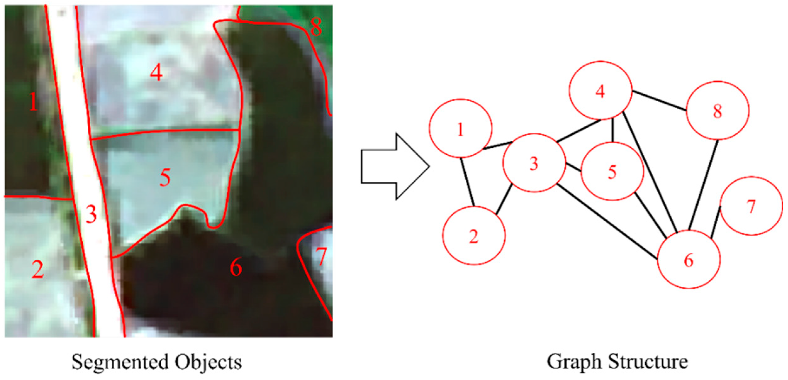
To utilize the graph convolutional network (GCN) for the identification task, the original data needed to be transformed into graph data format to meet the GCN’s requirement for graph-structured input. The example of constructing spatially correlated graph data based on GCN was illustrated in Figure 4. Each segmented object (1, 2, 3, 4, 5, 6, 7, 8 shown in Figure 4) was represented as a node in the graph, and the adjacency relationships between segmented objects were used to define edges in the graph. This approach effectively embedded the spatial relationships among segmented objects into the graph data, providing fundamental support for subsequent identification tasks [24].
In this study, the feature matrix was constructed using the optimal feature subset of the rice objects. As shown in Table 2, for a graph structure containing N nodes, the input feature matrix could be represented as f R N × M , M = M S + M T + M P + M t . Here, M s denoted the dimensionality of spectral features for the segmented objects, M T represented the dimensionality of texture features, M P corresponded to the dimensionality of polarization features, and M t indicated the dimensionality of terrain features.
The adjacency matrix was constructed as follows: first, a zero matrix of size N×N was initialized, where N represents the total number of segmented objects. Then, neighborhood analysis was performed on the segmented objects; if two objects were adjacent, the corresponding entry in the zero matrix was set to 1, indicating the presence of an edge connecting them. Table 3 showed the adjacency matrix created based on the graph structure example in Figure 4.

2.3.2. GCN Model Design

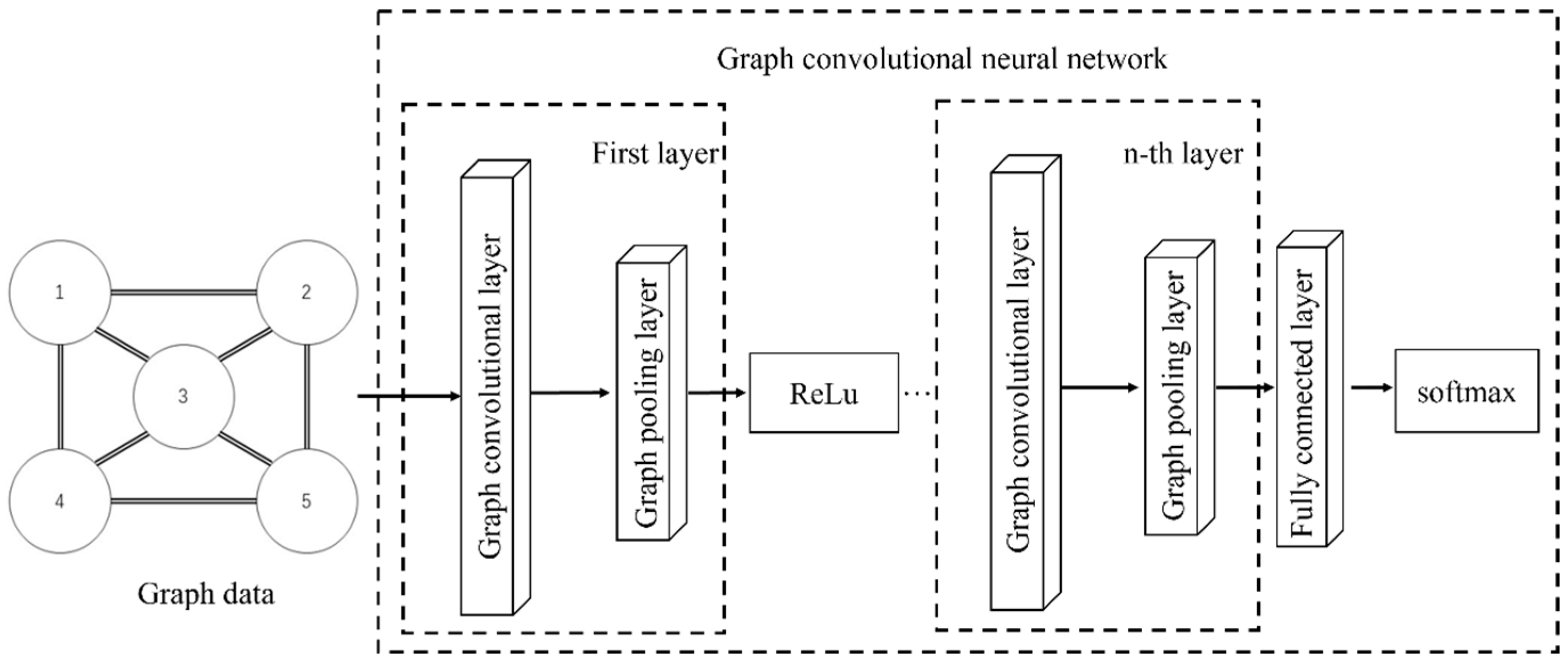
Section 2.3.1 briefly described the method for constructing graph convolutional network (GCN) data. This section focused on the design of the GCN architecture. The model primarily consisted of multiple graph convolutional layers, a fully connected layer, and a softmax classification layer. Specifically, each graph convolutional layer was further divided into two parts: the graph convolution operation and the pooling operation. Apart from receiving adjacency matrix inputs, this structure closely resembled the convolution and pooling layers found in conventional convolutional neural networks (CNNs). The overall architecture of the GCN is illustrated in Figure 5.
To fully leverage the advantages of the GCN model, this study explored and optimized the GCN structure from two aspects: first, the determination of the number of graph convolutional layers, and second, the selection of the neighborhood size k for nodes. The effects of these parameters on identification accuracy were analyzed separately. Experimental results demonstrated that the GCN model performed best with two graph convolutional layers, achieving the highest identification accuracy. Under this two-layer configuration, the accuracy peaked when the node neighborhood size k was set to 10. Therefore, this study adopted a GCN architecture with two graph convolutional layers and a neighborhood size k = 10, which was used consistently in subsequent experiments.

2.4. Accuracy Evaluation Methods

In remote sensing land cover classification experiments, accuracy assessment is a critical step for evaluating the reliability of the results. In this study, a combination of multiple evaluation methods was employed to comprehensively assess the classification accuracy. These methods included: generating a confusion matrix for accuracy evaluation [25], comparing statistical results of rice planting area, and conducting manual interpretation by comparing the classification results in local validation regions with high-resolution Google Earth imagery [26]. The evaluation focused on the following three aspects:
(1)
Confusion Matrix-Based Accuracy Assessment
The confusion matrix is a core metric for evaluating classification accuracy in remote sensing land cover classification experiments and is widely recognized as an objective and reliable evaluation method [27]. By statistically comparing the one-to-one correspondence between object classes in the reference and predicted imageries, it assesses class consistency and enables the calculation of various evaluation metrics, including producer accuracy, user accuracy, overall accuracy, and F1 Score.
Producer Accuracy (PA) measures the proportion of correctly classified objects in a particular land cover class relative to the total number of reference objects in that class. It is calculated as:
P A = t i v i × 100 %
where t i represents the number of correctly classified objects in class i , and v i is the total number of reference objects in that class.
User Accuracy (UA) reflects the proportion of correctly classified objects within a class relative to the total number of objects that were classified into that class. It is given by:
U A = t i m i × 100 %
where m i denotes the number of validation samples classified as class i .
F1 Score addresses the limitation of Overall Accuracy (OA), which only considers the diagonal elements of the confusion matrix. By integrating both precision and recall, the F1 Score offers a more comprehensive evaluation and serves as an important indicator of classification effectiveness. It is computed as:
F 1 = 2 × P A × U A P A + U A × 100 %
Overall Accuracy (OA) is defined as the ratio of correctly classified objects to the total number of validation objects. The total number is based on the reference land cover classification, which is determined from ground truth imagery or data from regions of interest. The diagonal elements of the confusion matrix represent correctly classified objects. The formula is:
O A = i = 1 n t i V × 100 %
where V is the total number of validation samples.
(2)
Comparative Analysis with Statistical Yearbook Data
The total rice planting area in the study region was obtained from the 2022 edition of the Study Region Statistical Yearbook, specifically from the agriculture section. These official statistics were compared with the rice area derived from the classification results of this study. This comparison enabled an assessment of the experimental accuracy from a quantitative perspective.
(3)
Visual Interpretation of Sample Regions
Manual visual interpretation was performed in selected regions of the classification results to assess the completeness of rice extraction and identify potential commission and omission errors. By subjectively analyzing the spatial consistency between the extracted rice distribution and high-resolution reference imagery, a comprehensive evaluation of classification accuracy and performance was conducted.

3. Experiments and Results

3.1. Study Area and Data

3.1.1. Study Area

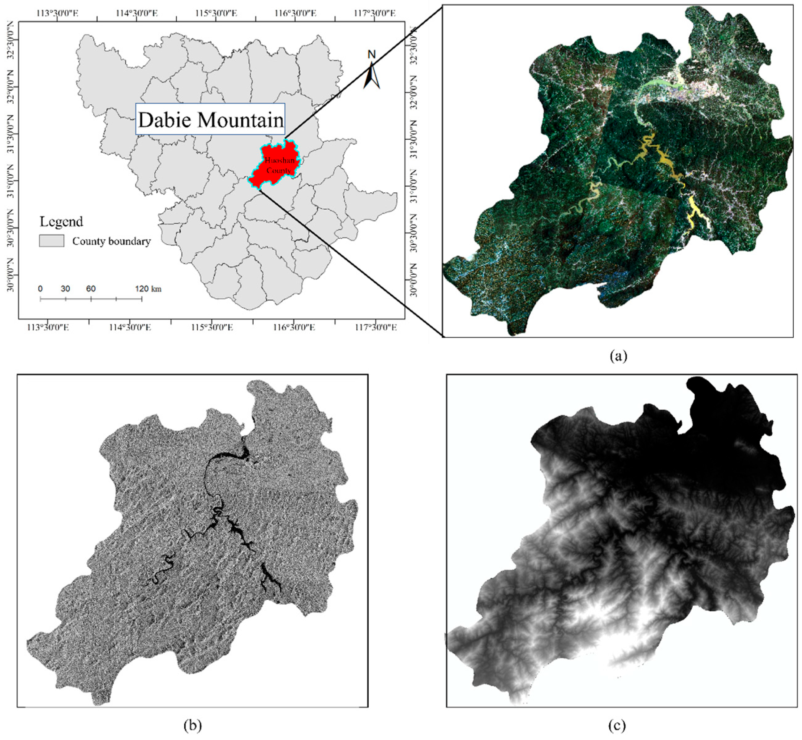
The study area is located in Huoshan County, situated in the Dabie Mountains in the central-eastern region of China (as shown in Figure 6). The Dabie Mountains span the provinces of Hubei, Henan, and Anhui, serving as the watershed between the Yangtze and Huai Rivers. The terrain is dominated by low- to mid-altitude mountains and hilly landscapes, with significant variations in elevation. The region experiences abundant rainfall, hosts numerous rivers, and possesses ample water resources, all of which provide favorable conditions for agricultural production. As one of the major staple crops, rice is widely distributed across river valley plains, intermountain basins, and some gently sloping terraces.
Huoshan County is located in the eastern part of the Dabie Mountains and is characterized by terrain that generally slopes from west to east. Mountainous and hilly areas cover the majority of the county’s land. Despite the significant topographic variation, rice cultivation in this region achieves high yields due to abundant water resources and favorable climatic conditions, making rice one of the most important staple crops in the area. Huoshan has also been designated as a key ecological agriculture demonstration zone in Anhui Province and has implemented a series of ecological agricultural policies to promote sustainable development and the green transformation of agricultural production [28]. Considering the widespread rice cultivation and the complex agricultural terrain in this region, Huoshan County was selected as the specific study area for this research.

3.1.2. Data

The data included the remote sensing data for the rice field identification and auxiliary data, as shown in Table 4.
(1)
Remote Sensing Data for the Rice field identification
Gaofen-2 multispectral imagery was selected as the remote sensing data for the rice field identification. With a spatial resolution of 1 m and a high revisit frequency, Gaofen-2 provides significant advantages for remote sensing monitoring in mountainous regions [29]. Due to Huoshan County’s mountainous location, Gaofen-2 imagery covering the area exhibited varying degrees of cloud cover throughout the entire rice growing season. This study used imagery acquired in June 2022, during the vegetative growth stage of rice. At this stage, rice growth is stable and the plants are vigorously developing, making them more distinguishable and easier to accurately identify in remote sensing imagery [30].
(2)
Auxiliary Data
① ALOS Topographic Data
ALOS topographic data were selected to provide terrain features for the rice field identification task. These data were derived from the PALSAR sensor onboard the ALOS satellite [31]. The ALOS data used in this study were acquired in July 2010, with the DEM data obtained under the Fine Beam Single (FBS) mode, achieving an actual spatial resolution of 12.5 m.
② Gaofen-3 SAR Imagery
Gaofen-3 SAR imagery was used for two primary purposes: (1) in the rice field identification task, it provided polarization features that helped distinguish rice from other land cover types; (2) in the cloud removal task, it supplied SAR features essential for the coarse cloud removal process. Gaofen-3 is China’s first C-band, multi-polarization, high-resolution synthetic aperture radar (SAR) satellite, offering up to 12 imaging modes [32]. The Gaofen-3 SAR data used in this study were acquired in June 2022.
③ Gaofen-1 Multispectral Imagery
Gaofen-1 multispectral imagery was used as the neighboring optical remote sensing imagery. Although Gaofen-1 has a lower spatial resolution (2 m) compared to Gaofen-2, it provided cloud-free optical imagery from a nearby period during the rice growth season, making it suitable for the cloud removal task in this study. The Gaofen-1 multispectral imagery used was acquired in July 2022.

3.2. Experimental Setup

3.2.1. Sample Dataset

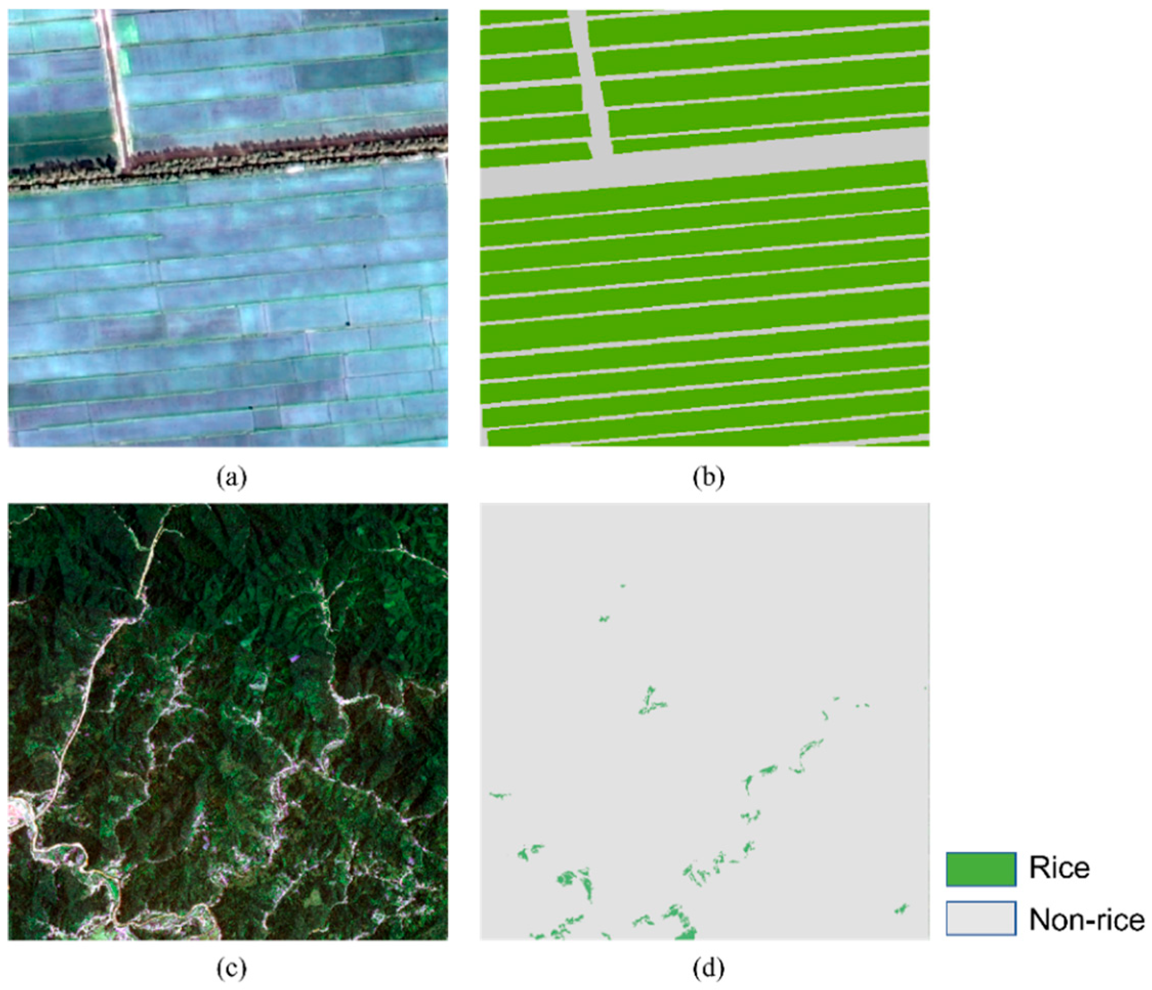
The rice field sample dataset used in this study consisted of two parts: a pre-trained dataset and a self-constructed dataset. Both datasets were derived from Gaofen-2 multispectral imagery and were visually interpreted with the assistance of high-resolution Google Earth imagery (0.3 m resolution). The pre-trained rice dataset contained 1,581 imageries, each with a size of 256×256 pixels, primarily representing rice planting areas in plains. The self-constructed dataset comprised 866 imageries of the same size, selected from rice-growing regions within Huoshan County. Both datasets were split into training and testing sets in an 8:2 ratio. All samples were normalized to reduce the effects of illumination and other environmental factors. The rice field sample examples are shown in Figure 7.

3.2.2. Experimental Environment and Parameter Settings

The experiments were conducted using the TensorFlow deep learning platform. The hardware configuration used in this study is listed in Table 5. The software environment included Microsoft Windows 10 as the operating system, Python 3.8 as the programming language, and TensorFlow_GPU 2.7.0 as the deep learning framework.
This study employed a GCN model for rice identification experiments, where the training parameter configuration played a decisive role in the final extraction accuracy. The loss function was set as cross-entropy loss, and the optimization algorithm used was the Adam optimizer. The number of epochs was set to 10,000 to ensure sufficient fitting of the network to the data. The learning rate was initialized at 0.001 with a decay schedule configured to gradually reduce the learning rate during training, thereby enhancing model optimization stability. To avoid memory overflow issues, the original dataset was divided into imagery blocks composed of several nodes for training. Among these, 75% were allocated as the training set and 25% as the validation set. From the training set, 6,000 samples were randomly selected for training, while 1,000 samples were randomly selected from the validation set for validation.

3.3. Results

3.3.1. Cloud Removal Results of the Optical Remote Sensing Imagery

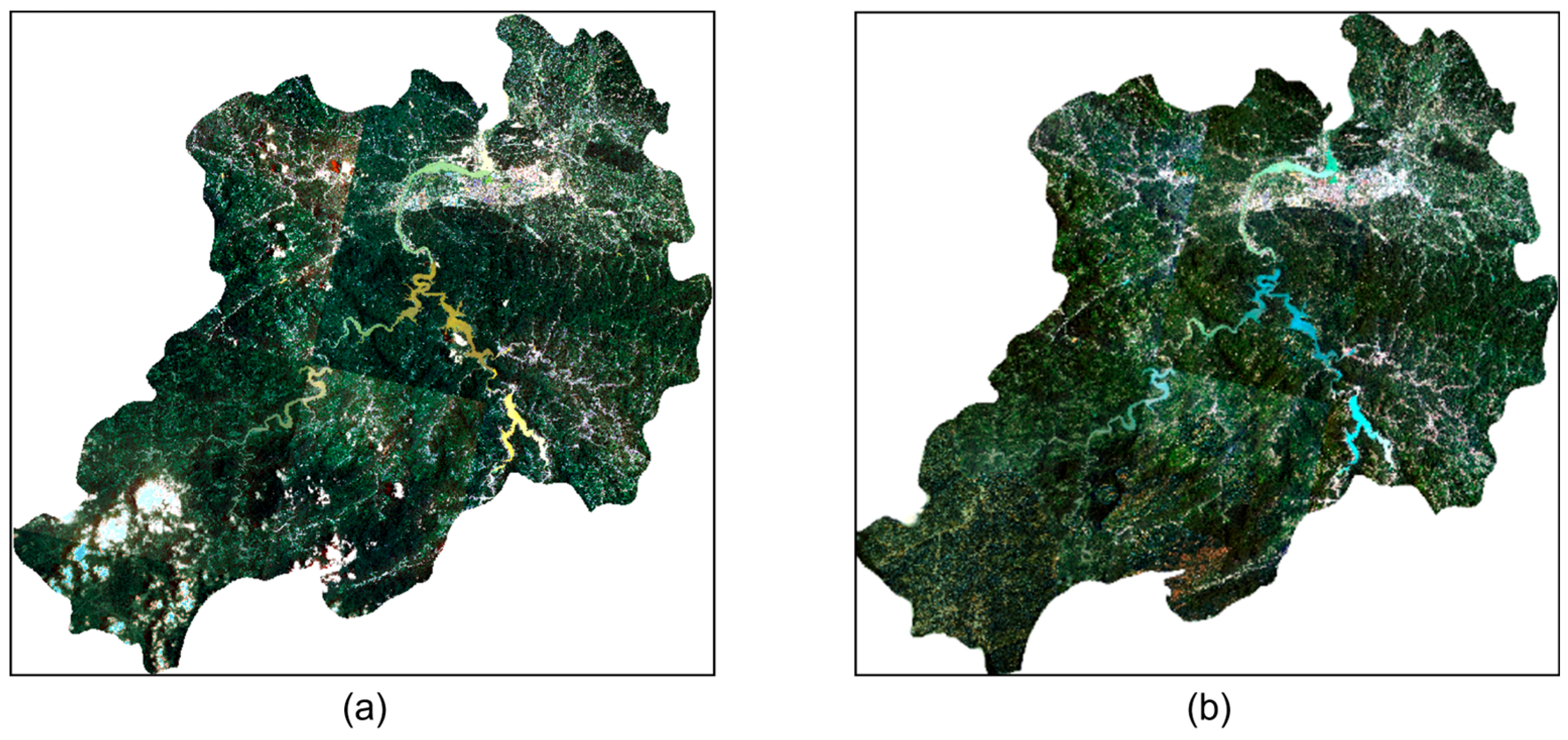
The cloud removal method proposed in this study was applied to the optical remote sensing imagery of Huoshan County, the study area. By effectively addressing the prevalent cloud cover issue in this region, the method successfully generated high-quality cloud-free imageries, thereby providing a reliable data foundation for subsequent rice field identification experiments. The cloud removal results were shown in Figure 8.

3.3.2. Feature Selection Results

Table 6 presented the results of the optimal feature subset. The spectral features dominated the subset, most of which were spectral indices calculated from near-infrared bands. This was because the rice crop exhibited the high reflectance and distinct differences from other land covers, which made the spectral features highly discriminative in identifying the rice field in mountainous regions. The texture features accounted for 26% of the total features. Due to the pronounced striping and regular arrangement characteristics of rice fields, these texture features demonstrated good capability in distinguishing rice fields from irregularly textured land covers, such as forests or shrubs.

3.3.3. Rice Field Identification Results

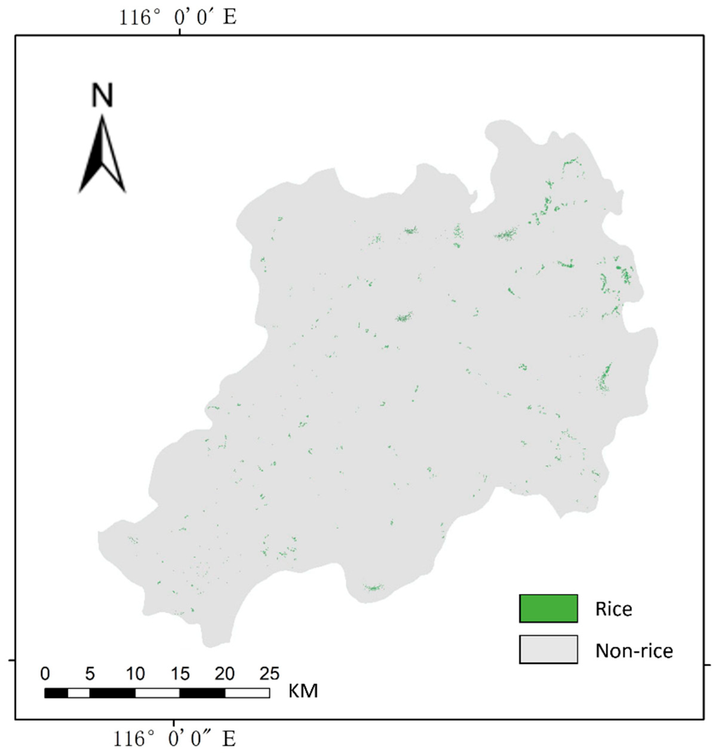
The graph-structured data of Huoshan County were input into the trained GCN model to identify the rice planting areas, and the results were visualized as shown in Figure 9. The identification accuracy is presented in Table 7. As shown in Table 7, the accuracy metrics of PA, UA, F1-Score, and OA were high.
To further verify the reliability of the identification results, the local region was visually interpreted by comparison with high-resolution Google Earth imagery, as shown in Figure 10. It can be observed that the rice fields can be correctly identified from easily confused land cover/use categories. This indicated that the proposed method had a low identification error, and the identified rice planting extent closely matched the actual distribution.
The results of the rice field identification were compared and analyzed against the data from the statistical yearbook. Table 8 showed the rice planting area extracted from the identification results and the corresponding data from the 2022 Huoshan County Statistical Yearbook. According to the yearbook, the rice planting area in Huoshan County in 2022 was 179.1 km2, while the proposed method estimated the rice planting area as 173.3 km2. The data matching rate had reached 96.8%.

4. Discussion

4.1. Ablation Study on Terrain Features

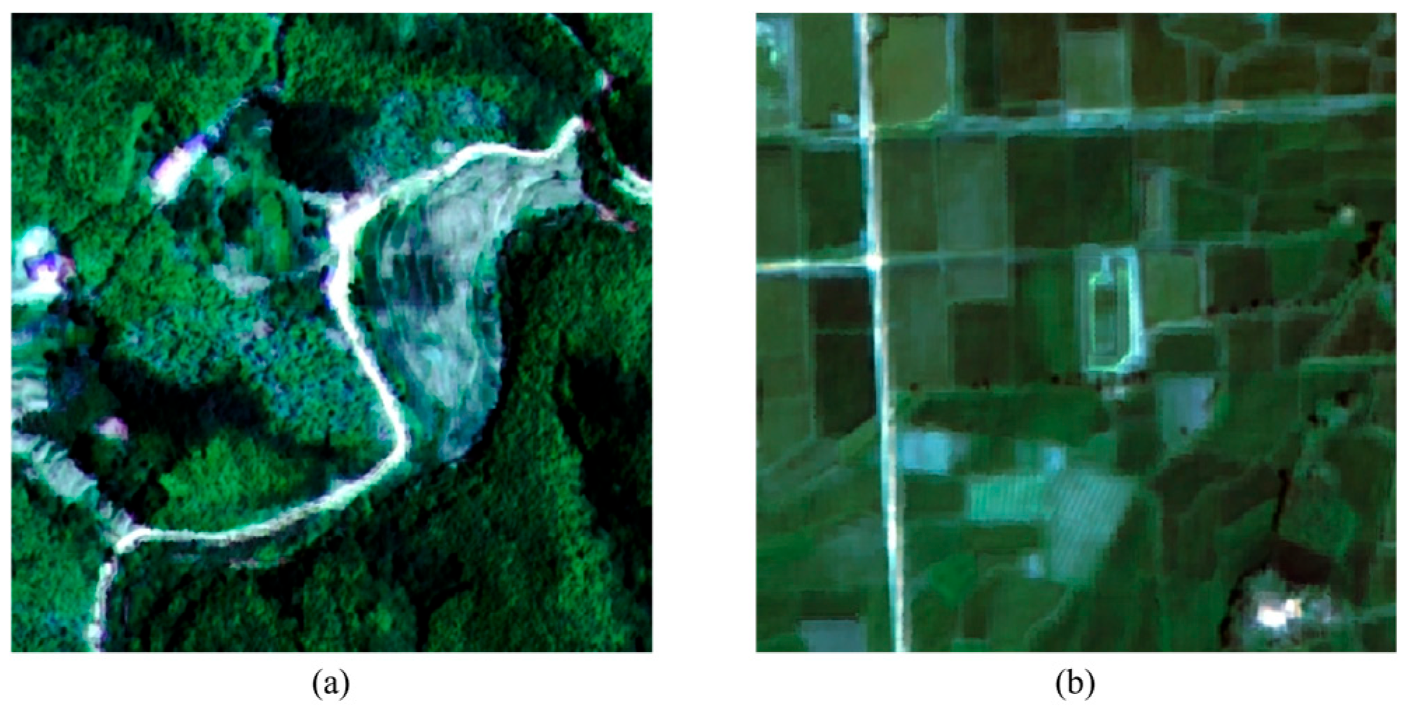
To verify the impact of terrain features on the rice field identification under mountainous conditions, we designed a series of ablation experiments. We kept the experimental data and extraction models unchanged, and trained the rice field identification models for both plain(the example shown in Figure 11b) and mountainous(the example shown in Figure 11a) regions without including terrain features. Then, we incorporated terrain features into the models and compared the rice field identification accuracy across the two geographic settings.
Among the 19 optimized features, we removed the two terrain features—slope and aspect—and input the remaining features into the GCN model for training to obtain the identification results. Then, we reintroduced the terrain features and retrained the model to acquire updated the identification results. Table 9 compared the identification accuracies before and after incorporating the terrain features. The results showed that the identification accuracy improvement after incorporating the topographic features was 3.8% in the mountainous region, while in the plain region, the corresponding improvement was only 0.2%. This quantitatively demonstrated the importance of terrain features for the rice field identification in mountainous regions, which can effectively reduce the misclassification and omission errors.
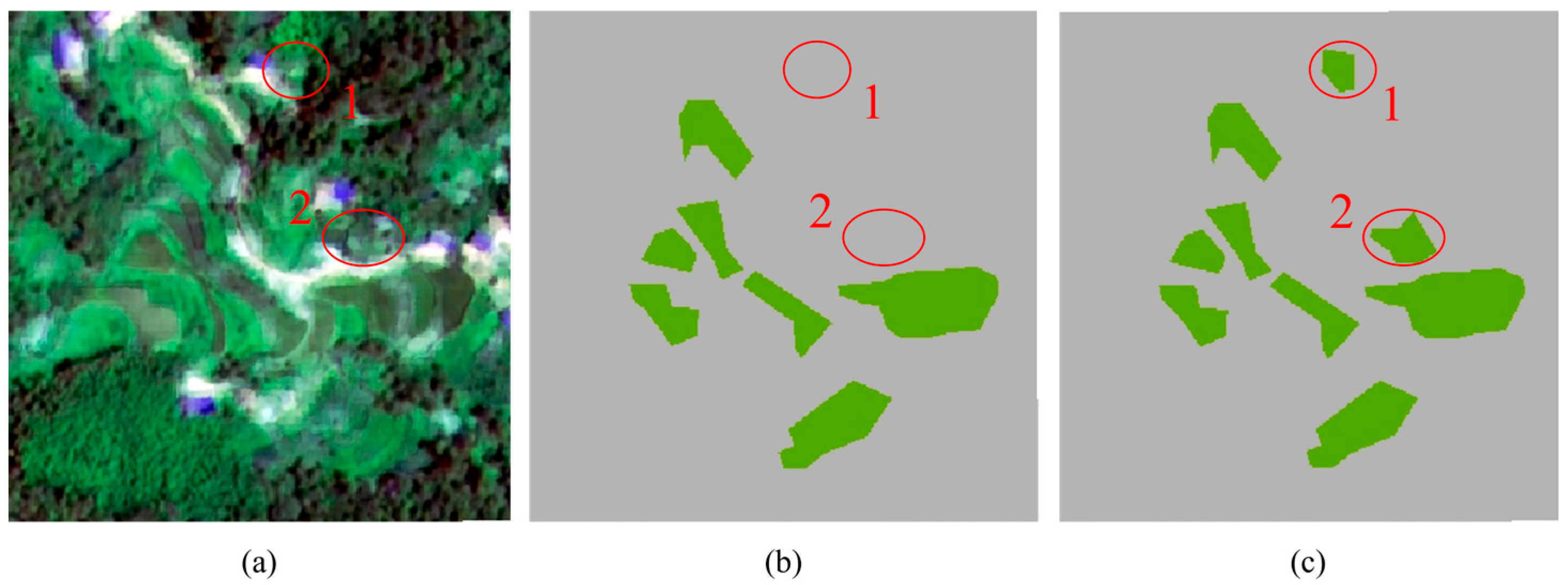
Figure 12 showed the local identification results without and with the terrain features in the mountainous region.We observed that Object 1 and 2 were not identified in Figure 12b, but were successfully identified in Figure 12c. Object 1 and 2 was near the boundaries between the mountains and plains. This was partly due to the abundance of trees in the mountainous region, whose spectral characteristics closely resemble those of rice, making it difficult for other features to distinguish between these land cover types and resulting in the omissions of the rice fields along the edges. After incorporating terrain features such as slope and aspect, the model’s identification performance under complex terrain conditions were improved significantly. These terrain features provided the crucial spatial context, and enabled the model to more accurately differentiate rice from other land covers.

4.2. Comparison with Other Methods

Using the same sample dataset and feature set, we applied two machine learning methods—Support Vector Machine (SVM) [33] and Random Forest (RF) [34]—alongside the deep learning model U-Net [35] to identify the rice planting areas in Huoshan County. We then compared the results of these methods with our results.

4.2.1. Overall Accuracy Comparison

We compared the rice field identification accuracy of four methods across the entire study area, as summarized in Table 10. The results showed that the overall accuracy (OA) achieved by our proposed method significantly outperformed the other three classification algorithms. This demonstrated its superior performance for the rice field identification.
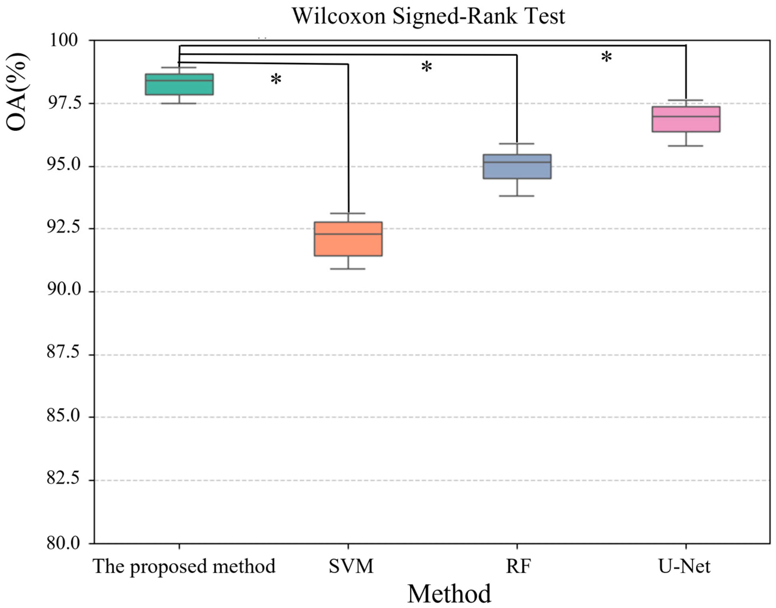
Due to the limited number of rice field samples in mountainous regions, the experimental results may be affected by random data fluctuations. To verify whether the overall accuracy advantage of the proposed method was statistically significant rather than due to chance, we conducted the Wilcoxon Signed-Rank Test. This non-parametric test compared paired samples, where a p-value less than 0.05 indicated that the accuracy improvement of our method over comparative approaches was statistically significant, confirming its reliability. We selected 20 test regions and used the overall accuracy (OA) of each method within each region as paired samples. The p-values comparing our method with SVM, RF, and U-Net were calculated. Accuracy distributions for each method were visualized via box plots and interpreted alongside the significance test results to assess the statistical meaningfulness of the observed improvements.
The statistical significance of the differences between the proposed method and the comparison methods (SVM, RF, and U-Net) was assessed using the Wilcoxon signed-rank test at a significance level of 0.05. As summarized in Table 11, all comparisons yielded p-values below 0.05 (p < 0.05), which indicated that the improvements in overall accuracy (OA) achieved by the proposed method were statistically significant. Figure 13 presented the box plots of the OA distributions for the four methods across different test regions, where statistically significant differences were marked by asterisks (*). The proposed method consistently demonstrated higher accuracy and greater stability, which was reflected by its smaller interquartile range (IQR), indicating reduced variability in the results. These findings collectively confirmed the robustness and superiority of the proposed method for the rice ifield dentification in mountainous regions.unit

4.2.2. Local Performance Comparison

The overall accuracy of the four methods across the entire study area had been presented above. To visually compare their classification performance in local regions, three representative regions were selected from the validation set. The rice field identification results for these regions, based on the four methods, were shown in Figure 14.
To ensure a fair comparison, all four methods were evaluated under identical conditions using object-based rice classification. This approach avoids issues such as mixed pixels and unclear boundaries, focusing instead on the accurate identification of rice objects. Region A features relatively flat terrain with forests, bare land, roads, and rice fields. Here, SVM and RF misclassified many bare land and forest areas as rice, likely due to their limited feature learning capacity and difficulty in balancing multiple feature classes, resulting in disordered identification outcomes. U-Net produced results similar to ours, as its deep feature extraction effectively captures rice characteristics, performing well in flat terrain but still missing some rice areas, possibly due to overfitting from model complexity. Region B represents typical mountainous terrain, primarily comprising forest, bare land, and rice. In this area, SVM and RF exhibited increased misclassification, tending to overestimate rice planting areas relative to the actual distribution. U-Net showed notable omission errors, as the spectral similarity between rice and adjacent forest areas caused misidentification. In contrast, our method accurately identified rice fields by emphasizing spatial relational features between land objects, which U-Net did not fully capture. Region C is a relatively flat area with pronounced spectral differences between land types. While SVM and U-Net both showed some omission and commission errors, U-Net’s strong deep feature representation enabled successful identification of all rice units. Our method also identified all rice fields, which demonstrated its capability to effectively integrate multiple feature types. In summary, particularly in the complex mountainous terrain, our method leverages spatial relational features among land objects to precisely identify rice fields, and outperformed the other three methods.

4.2.3. Terrain Adaptability Comparison

To verify whether the proposed method can effectively utilize spatial relationships to improve rice field identification accuracy in mountainous terrain compared to the other three methods, the study area was divided into three slope categories based on slope values derived from the DEM: low slope (<10°), medium slope (10–30°), and high slope (>30°). The performance of each method was then evaluated separately within these slope classes. Although SVM and RF employed multiple feature types, they lacked the ability to leverage spatial features. The U-Net models were tested with convolution kernels of sizes 3 × 3, 5 × 5, and 7 × 7 to assess the effect of receptive field size, with the 5 × 5 kernel producing the best results. In contrast, our proposed method constructed graph structures based on adjacency matrices, which enabled the extraction of spatial topological information. Table 12 demonstrated that the proposed method achieved the most significant improvement in identification accuracy under the high-slope conditions, which outperformed SVM by 13.5%, RF by 10.9%, and U-Net by 7.4%. This finding indicates that incorporating spatial relational features between rice field units effectively enhances the rice field identification accuracy under complex mountainous terrain conditions. While U-Net performed better under the low-slope conditions due to its deep feature extraction being well-suited for simpler terrains, its accuracy declined sharply under the high-slope conditions, which reflected the limited adaptability of fixed receptive fields to complex topography. In contrast, both SVM and RF exhibited relatively poor performance under all slope conditions. This suggested that methods lacking the ability to leverage spatial information struggle to achieve satisfactory identification results under complex mountainous conditions.

4.2.4. Comparison of Training Sample Requirements

In mountainous regions, rice field distribution tends to be sparse, and labeled data are often limited. To evaluate whether the proposed method demonstrates greater robustness compared to SVM, RF, and U-Net under small-sample training conditions, we kept the test set unchanged and conducted experiments using 100%, 75%, and 50% of the training samples. For SVM and RF, classifiers were directly trained with the reduced training sets. U-Net was trained using a standard fully supervised approach, with data augmentation applied to alleviate the issue of limited samples. Our proposed method leveraged adjacency information for semi-supervised training, which enabled feature learning from neighboring nodes even when some nodes lacked labels.
Table 13 showed that when the training samples were reduced to 50%, the identification accuracy of the proposed method decreased by only 10.3%, while SVM and RF experienced declines exceeding 24%, and U-Net dropped by 16.3%. This demonstrated that our method can effectively leverage limited labeled data for identification. In contrast, SVM and RF heavily depended on the quantity of training samples and suffer from severe overfitting when samples were insufficient. Similarly, U-Net, which strongly relied on supervised samples, also exhibited a significant decrease in identification accuracy under limited data conditions.

4.2.5. Comparison of Computational Costs

To accurately identify scattered rice field units in mountainous regions, this study utilized high spatial resolution imagery. However, the use of high-resolution imageries inevitably leads to a significant increase in computational cost, demanding that the model possess efficient computing capabilities and optimization strategies. To assess the computational efficiency of the proposed method compared to other approaches, prediction times were measured on imagery blocks of sizes 256 × 256 and 512 × 512 pixels, and the number of model parameters was recorded. As traditional classifiers, SVM and RF require relatively low computational resources; U-Net, built upon deep convolutional architectures, incurs high computational overhead; while GCN, which models data through graph structures, exhibits computational complexity intermediate between the two.
Table 14 demonstrated that the proposed method’s prediction speed was approximately 40% of that of U-Net, while utilizing fewer model parameters. This indicates that our method effectively reduces computational overhead without sacrificing identification accuracy, making it more suitable for processing large-scale high-resolution remote sensing imageries. In contrast, U-Net’s deeper network architecture results in longer computation times, limiting its practicality for large-area high-resolution applications. Although SVM and RF offer faster prediction speeds, their identification accuracy is substantially lower than that of deep learning-based methods, rendering them less effective for fine-grained classification tasks.

4.3. Key Advances and Highlights

The proposed method made several notable contributions to rice field identification in mountainous regions.
First, in terms of feature extraction, a systematic design was carried out according to the growth characteristics of rice and the complexity of mountainous terrain. Spectral features were derived from multiple vegetation indices, which effectively reflected the physiological and biochemical traits of rice (e.g., chlorophyll content, biomass, and vegetation coverage). These indices also reduced the influence of soil background and atmospheric conditions, thereby enhancing the discriminative power of rice signals [36,37]. Texture features captured the spatial patterns of paddy fields, which played an important role in distinguishing rice from other crops [38]. Polarization features, obtained from radar backscatter differences, further improved the separability between rice and other vegetation types [39]. Moreover, topographic features accounted for environmental constraints specific to mountainous conditions, such as elevation, slope, and aspect, which directly influenced water availability, illumination, and temperature gradients, thereby affecting the growth cycle and spatial distribution of rice [40]. The integration of these multidimensional features not only improved classification accuracy but also provided a representation more consistent with the ecological reality of rice in mountainous regions.
Second, in the model construction, the conventional graph convolutional network (GCN) architecture was customized for rice field identification. Superpixels (representing rice units) were used as graph nodes, and multi-source features were integrated into the graph structure, which effectively captured the complex spatial relationships of rice distribution in mountainous regions. These structural enhancements addressed the insufficient utilization of multi-dimensional features observed in previous studies, resulting in high-precision identification of rice fields under mountainous conditions and notable improvements in computational efficiency. Compared with traditional classifiers, the proposed method demonstrated a better ability to adapt to the spatial characteristics of rice distribution in complex terrain, providing an efficient and reliable approach for rice field identification in mountainous regions [41,42].
In addition, the proposed method demonstrated strong transferability. On the one hand, the data used in this study were not restricted to a specific region, making the approach applicable to both plain and mountainous regions. On the other hand, topographic factors were represented using a digital elevation model (DEM), which did not impose special requirements on slope gradients or landform types. Therefore, the method can be applied under various terrain conditions and across different regions, offering a valuable reference for large-scale rice field identification and monitoring.

4.4. Limitations and Future Research

This study proposed a rice field identification method under mountainous conditions, which could be effectively applied to high-resolution remote sensing imagery in mountainous rice-planting areas and achieved satisfactory identification results. However, several aspects remained to be improved.
(1) The cloud removal method based on the fusion of SAR and neighboring optical remote sensing imageries did not impose strict theoretical requirements on the selection of neighboring optical imageries. In principle, any cloud-free optical imagery acquired within the same rice growth stage could serve as neighboring imagery. In practice, however, neighboring optical imageries derived from different sensors, with varying spatial resolutions and spectral characteristics, might affect the cloud removal performance [43]. Future studies could investigate the influence of these factors on cloud removal results and attempt to establish criteria for the optimal selection of neighboring optical imageries.
(2) The rice field identification experiments in this study were conducted only in Huoshan County of the Dabie Mountains. Huoshan County is characterized by a typical mountainous terrain, with extensive rice cultivation, making it representative to a certain extent. Nevertheless, differences in topographic relief, elevation, and rice distribution across regions may influence the identification results [44]. Future research could expand the experimental scope to broader areas and incorporate transfer learning techniques to enhance the generalization capability of the proposed method, thereby further verifying its applicability across the Dabie Mountains and providing stronger technical support for precision agriculture monitoring in mountainous regions.

5. Conclusion

This study proposed a rice field identification method specifically designed for mountainous conditions, effectively leveraged multi-dimensional feature information to enhance identification performance. Compared with existing approaches, the proposed method demonstrated superior accuracy and broader applicability. The main conclusions are summarized as follows:
  • A coarse-to-fine cloud removal strategy was implemented, which comprehensively integrated features from SAR imagery and neighboring temporal optical remote sensing imageries to achieve effective cloud removal from optical data. The method achieved high performance and outperformed alternative methods in both accuracy and applicability.
  • By fully accounting for the growth environment and spatial distribution characteristics of rice in mountainous terrain, and by integrating multi-source features through graph structure modeling, the proposed approach successfully addressed the limitations of existing methods in handling complex terrain. This led to significant improvements in identification accuracy and model robustness.

Author Contributions

Conceptualization, Y.W.; Methodology, Y.W., Z.Y. and W.Z.; Validation, Z.Y.; Investigation, W.Z.; Resources, J.C. and Z.Y.; Data curation, Y.W.; Writing—original draft, J.C. and W.Z.; Writing—review & editing, W.Z.; Visualization, W.Z.; Project administration, Z.Y.; Funding acquisition, J.C. and Z.Y. All authors have read and agreed to the published version of the manuscript.

Funding

This research was funded by the National Natural Science Foundation of China (No. 41671514), the Surveying and mapping science and technology “double first-class” discipline creation project (No. GCCYJ202409, No. BZXCG202403), and the Natural Science Foundation of Henan Province (No. 162300410122).

Data Availability Statement

The original contributions presented in this study are included in the article. Further inquiries can be directed to the corresponding author.

Conflicts of Interest

The authors declare no conflicts of interest.

References

  1. Rezaei, E.E.; Webber, H.; Asseng, S.; Boote, K.; Durand, J.L.; Ewert, F.; Martre, P.; MacCarthy, D.S. Climate change impacts on crop yields. Nat. Rev. Earth Environ. 2023, 4, 831–846. [Google Scholar] [CrossRef]
  2. Yang, H.; Pan, B.; Wu, W.; Tai, J. Field-based rice classification in Wuhua county through integration of multi-temporal Sentinel-1A and Landsat-8 OLI data. Int. J. Appl. Earth Obs. Geoinf. 2018, 69, 226–236. [Google Scholar] [CrossRef]
  3. Pang, J.; Zhang, R.; Yu, B.; Liao, M.; Lv, J.; Xie, L.; Li, S.; Zhan, J. Pixel-level rice planting information monitoring in Fujin City based on time-series SAR imagery. Int. J. Appl. Earth Obs. Geoinf. 2021, 104, 102551. [Google Scholar] [CrossRef]
  4. Estacio, I.; Basu, M.; Sianipar, C.P.; Onitsuka, K.; Hoshino, S. Dynamics of land cover transitions and agricultural abandonment in a mountainous agricultural landscape: Case of Ifugao rice terraces, Philippines. Landsc. Urban Plan. 2022, 222, 104394. [Google Scholar] [CrossRef]
  5. Zhao, S.; Liu, X.; Ding, C.; Liu, S.; Wu, C.; Wu, L. Mapping Rice Paddies in Complex Landscapes with Convolutional Neural Networks and Phenological Metrics. GISci. Remote Sens. 2019, 57, 37–48. [Google Scholar] [CrossRef]
  6. Nduati, E.; Sofue, Y.; Matniyaz, A.; Park, J.G.; Yang, W.; Kondoh, A. Cropland Mapping Using Fusion of Multi-Sensor Data in a Complex Urban/Peri-Urban Area. Remote Sens. 2019, 11, 207. [Google Scholar] [CrossRef]
  7. Jing, W.; Huang, J.; Zhang, K.; Li, X.; She, B.; Wei, C.; Gao, J.; Song, X. Rice Fields Mapping in Fragmented Area Using Multi-Temporal HJ-1A/B CCD Images. Remote Sens. 2015, 7, 3467–3488. [Google Scholar]
  8. Quan, J.; Wang, Y.; Wang, X.; Tang, W.; Wang, Q. Extraction of rice planting areas in the Dabie Mountains using remote sensing images: A case study of Landsat 8. Chin. Agric. Sci. Bull. 2019, 35, 104–111. [Google Scholar]
  9. Sang, G.; Tang, Z.; Mao, K.; Deng, G.; Wang, J.; Li, J. Extraction of high-resolution rice planting areas based on GEE cloud platform and Sentinel data: A case study of Hunan Province. Acta Agron. Sin. 2022, 48, 2409–2420. [Google Scholar]
  10. Zhang, K.; Chen, Y.; Zhang, B.; Hu, J.; Wang, W. A Multitemporal Mountain Rice Identification and Extraction Method Based on the Optimal Feature Combination and Machine Learning. Remote Sens. 2022, 14, 5096. [Google Scholar] [CrossRef]
  11. Liu, W.; Wang, J.; Luo, J.; Wu, Z.; Chen, J.; Zhou, Y.; Sun, Y.; Shen, Z.; Xu, N.; Yang, Y. Farmland Parcel Mapping in Mountain Areas Using Time-Series SAR Data and VHR Optical Images. Remote Sens. 2020, 12, 3733. [Google Scholar] [CrossRef]
  12. Chen, A.; Li, Y. Rice identification at different growth stages in the southwest mountainous region based on Sentinel-2 imagery. Trans. Chin. Soc. Agric. Eng. 2020, 36, 8–15. [Google Scholar]
  13. Zhang, W.; Liu, H.; Wu, W.; Zhan, L.; Wei, J. Mapping rice paddy based on machine learning with Sentinel-2 multi-temporal data: Model comparison and transferability. Remote Sens. 2020, 12, 1620. [Google Scholar] [CrossRef]
  14. You, J.; You, S.; Tong, Y.; Li, J.; Pan, L.; Liu, H.; Zhang, L. A geostatistical approach for correcting bias in rice remote sensing identification. Trans. Chin. Soc. Agric. Eng. 2013, 29, 11–18. [Google Scholar]
  15. Ma, H.; Wang, L.; Sun, W.; Yang, S.; Gao, Y.; Fan, L.; Yang, G.; Wang, Y. A new rice identification algorithm under complex terrain combining multi-characteristic parameters and homogeneous objects based on time series dual-polarization synthetic aperture radar. Front. Ecol. Evol. 2023, 11, 1093454. [Google Scholar] [CrossRef]
  16. Chen, J.; Zhang, J.; Duan, Y.; Yang, Z.; Xia, X. A review of cloud detection and thick cloud removal in medium-resolution remote sensing imagery. Remote Sens. Technol. Appl. 2023, 38, 143–155. [Google Scholar]
  17. Li, Y.; Hong, D.; Li, C.; Yao, J.; Chanussot, J. HD-Net: High-resolution decoupled network for building footprint extraction via deeply supervised body and boundary decomposition. ISPRS J. Photogramm. Remote Sens. 2024, 209, 51–65. [Google Scholar] [CrossRef]
  18. Xiao, M.; Li, X.; Zhang, X.; Zhang, L. An image segmentation algorithm based on multi-scale region growing. J. Jilin Univ. (Eng. Technol. Ed.) 2017, 47, 1591–1597. [Google Scholar]
  19. Alirezapour, H.; Mansouri, N.; Zade, B.M.H. A Comprehensive Survey on Feature Selection with Grasshopper Optimization Algorithm. Neural Process. Lett. 2024, 56, 28. [Google Scholar] [CrossRef]
  20. Kong, Y.; Ni, D. Semi-Supervised Classification of Wafer Map Based on Ladder Network. In Proceedings of the 2018 14th IEEE International Conference on Solid-State and Integrated Circuit Technology (ICSICT), Qingdao, China, 31 October–3 November 2018. [Google Scholar]
  21. Robnik-Šikonja, M.; Kononenko, I. Theoretical and Empirical Analysis of ReliefF and RReliefF. Mach. Learn. 2003, 53, 23–69. [Google Scholar] [CrossRef]
  22. Zhou, J.; Huang, S.; Zhou, T.; Armaghani, D.J.; Qiu, Y. Employing a genetic algorithm and grey wolf optimizer for optimizing RF models to evaluate soil liquefaction potential. Artif. Intell. Rev. 2022, 55, 5673–5705. [Google Scholar] [CrossRef]
  23. Zuo, X.; Lu, H.; Zhang, Y.; Cheng, J.; Guo, Y. Graph convolutional network method for small-sample classification of hyperspectral imagery. Acta Geod. Cartogr. Sin. 2021, 50, 1358–1369. [Google Scholar]
  24. Hong, D.; Gao, L.; Yao, J.; Zhang, B.; Plaza, A.; Chanussot, J. Graph Convolutional Networks for Hyperspectral Image Classification. IEEE Trans. Geosci. Remote Sens. 2021, 59, 5966–5978. [Google Scholar] [CrossRef]
  25. Zhu, C.; Li, D.; Shao, Z.; Yin, J.; Wang, J. Evaluation method for segmentation accuracy of high-resolution remote sensing imagery based on object-oriented approach. High Power Laser Part. Beams 2015, 27, 43–49. [Google Scholar]
  26. Chen, Y.; Mo, W.; Mo, J.; Wang, J.; Zhong, S. Extraction of rice planting areas in southern China based on object-oriented classification. Remote Sens. Technol. Appl. 2011, 26, 163–168. [Google Scholar]
  27. Zhang, K.; Su, H.; Dou, Y. A novel method for evaluating classification accuracy of multi-class tasks based on confusion matrix. Comput. Eng. Sci. 2021, 43, 1910–1919. [Google Scholar]
  28. Chen, X.; Tang, L.; Wang, Z. Research on the current situation and countermeasures of characteristic agricultural development in Huoshan County. Shanxi Agric. Econ. 2022, 22, 147–149. [Google Scholar]
  29. Sun, W.; Yang, G.; Chen, C.; Chang, M.; Huang, K.; Meng, X.; Liu, L. Current status and literature analysis of Earth observation remote sensing satellite development in China. J. Remote Sens. 2020, 24, 479–510. [Google Scholar]
  30. Shan, J.; Wang, Y.; Liu, J.; Zhao, Y.; Li, Y. Monitoring rice planting areas based on multi-temporal Gaofen-1 satellite imagery. Jiangsu Agric. Sci. 2017, 45, 229–232. [Google Scholar]
  31. Cao, M.; Shi, Z.; Shen, Q. Study on optimal band selection of ALOS imagery in land cover classification. Bull. Surv. Mapp. 2008, 12, 16–18+27. [Google Scholar]
  32. Chen, Z.; Zhang, Q.; Chi, T.; Fu, W.; Li, C. Gaofen-3 satellite system and its applications. Satell. Appl. 2024, 2, 20–26. [Google Scholar]
  33. Wang, Z.; Wang, M.; Huang, Y.; Li, Y. A review on remote sensing image classification using support vector machine. Comput. Sci. 2016, 43, 11–17+31. [Google Scholar]
  34. Ma, Y.; Jiang, Q.; Meng, Z.; Li, Y.; Wang, D.; Liu, H. Land use classification of agricultural areas based on random forest algorithm. Trans. Chin. Soc. Agric. Mach. 2016, 47, 297–303. [Google Scholar]
  35. He, H.; Yang, G.; Li, H.; Feng, H.; Xu, B.; Wang, L. Water body extraction from high-resolution remote sensing imagery based on improved U-Net network. Geo-Inf. Sci. 2020, 22, 2010–2022. [Google Scholar]
  36. Guan, X.; Huang, C.; Liu, H.; Meng, X.; Liu, Q. Mapping rice cropping systems in Vietnam using an NDVI-based time-series similarity measurement based on DTW distance. Remote Sens. 2016, 8, 19. [Google Scholar] [CrossRef]
  37. Guan, S.; Fukami, K.; Matsunaka, H.; Okami, M.; Takahashi, K. Assessing correlation of high-resolution NDVI with fertilizer application level and yield of rice and wheat crops using small UAVs. Remote Sens. 2019, 11, 112. [Google Scholar] [CrossRef]
  38. Akbari, E.; Boloorani, A.; Samany, N.N.; Hamzeh, S.; Pignatti, S. Crop mapping using random forest and particle swarm optimization based on multi-temporal Sentinel-2. Remote Sens. 2020, 12, 1449. [Google Scholar] [CrossRef]
  39. Sun, C.; Zhang, H.; Ge, J.; Wang, C.; Li, L.; Xu, L. Rice mapping in a subtropical hilly region based on Sentinel-1 time series feature analysis and the dual branch BiLSTM model. Remote Sens. 2022, 14, 3213. [Google Scholar] [CrossRef]
  40. Zhu, W.; Pan, Y.; Hu, Z.; Jin, Y.; Bai, Y. Decline in planting areas of double-season rice by half in southern China over the last two decades. Remote Sens. 2024, 16, 440. [Google Scholar] [CrossRef]
  41. Gui, B.; Song, C.; Li, Y.; Wang, J.; Shang, S. SAGRNet: A novel object-based graph convolutional neural network for diverse vegetation cover classification in remotely-sensed imagery. ISPRS J. Photogramm. Remote Sens. 2025, 227, 99–124. [Google Scholar] [CrossRef]
  42. Jiang, H.; Zhang, C.; Qiao, Y.; Zhang, Z.; Meng, W. CNN feature based graph convolutional network for weed and crop recognition in smart farming. Comput. Electron. Agric. 2020, 174, 105450. [Google Scholar] [CrossRef]
  43. Gao, J.; Yuan, Q.; Li, J.; Zhang, H.; Su, X. Cloud removal with fusion of high resolution optical and SAR images using generative adversarial networks. Remote Sens. 2020, 12, 191. [Google Scholar] [CrossRef]
  44. Tian, X.; Zhou, Q.; Wang, L.; Feng, H.; Yang, P. Crop classification in mountainous areas using object-oriented methods and multi-source data: A case study of Xishui County, China. Agronomy 2023, 13, 3037. [Google Scholar] [CrossRef]
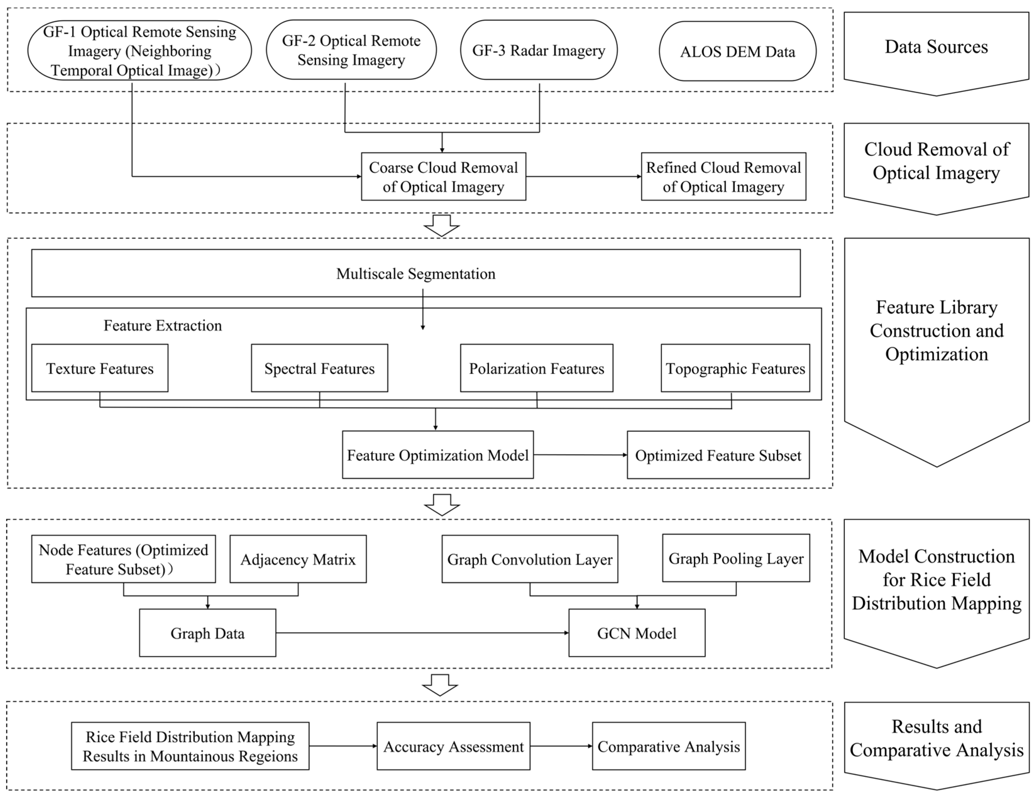
Figure 1. The Flowchart of the Proposed Framework.
Remotesensing 17 03356 g001
Figure 2. The Overall Workflow of the Optical Remote Sensing Imagery Cloud Removal Method.
Remotesensing 17 03356 g002
Figure 3. The Flowchart of the GWO_RF Algorithm.
Remotesensing 17 03356 g003
Figure 4. The Example of Constructing Spatially Correlated Graph Data.
Remotesensing 17 03356 g004
Figure 5. The Graph Convolutional Network Structure.
Remotesensing 17 03356 g005
Figure 6. The Study Area and Data: (a) GF-2 Multispectral Imagery; (b) GF-3 Radar Imagery; (c) Global ALOS 12 m DEM Imagery.
Remotesensing 17 03356 g006
Figure 7. The Rice Field Sample Examples: (a) Pre-trained Imageries; (b) Pre-trained Labels; (c) Self-constructed Imageries; (d) Self-constructed Labels.
Remotesensing 17 03356 g007
Figure 8. The Cloud Removal Results of the Optical Remote Sensing Imagery: (a) Original Cloud-covered Imagery; (b) Cloud-free Imagery.
Remotesensing 17 03356 g008
Figure 9. Rice field identification results.
Remotesensing 17 03356 g009
Figure 10. The Identification Result of the local region: (a) Google High-Resolution Imagery; (b) Original Imagery; (c) Identification Result.
Remotesensing 17 03356 g010
Figure 11. The Example of the Plain and Mountainous Region: (a) Mountainous region; (b) Plain Region.
Remotesensing 17 03356 g011
Figure 12. The Local Identification Results without and with the Terrain Features in the Mountainous Region: (a) Original Imagery; (b) The identification result Without the Terrain Features; (c) The identification result With the Terrain Features.
Remotesensing 17 03356 g012
Figure 13. The Box Plot of the OA Distributions for the Four Methods (The significance level was set at α = 0.05. An asterisk denotes a significant difference (* p < 0.05) between the proposed method and a comparator).
Remotesensing 17 03356 g013
Figure 14. The Rice Field Identification Results of the Local Regions Using the Four Methods.
Remotesensing 17 03356 g014
Table 1. The List of the Initial Feature Set.
Feature TypeFeature Description
Spectral FeaturesB1, B2, B3, B4, NDVI, CARI, RVI, DVI, EVI, SAVI, DNWI, VARI, PCA1, PCA2, HSV spectral-spatial features (12 types)
Texture FeaturesEntropy, Energy, Autocorrelation, Contrast, Dissimilarity, Variance, Small Gradient Dominance, Large Gradient Dominance, Uneven Distribution of Gray Levels, Uneven Distribution of Gradients, Gradient Energy, Gradient Variance, Correlation, Gray-level Entropy, Gradient Entropy, Mixed Entropy
Polarization FeaturesHH, VV, HV, VH
Terrain FeaturesDEM, Aspect, Slope, Curvature
Table 2. The Example of Feature Matrix X.
FeaturesFeature 1, Feature 2, …, Feature M
Object ID Spectral FeaturesTexture FeaturesPolarization FeatureTopographic Features
1
2
N
Table 3. Example of Adjacency Matrix A.
Object
Object
01100000
10100000
11011100
00101101
00110100
00111011
00000100
00010100
Table 4. The Overview of the Data.
Data TypeSourceAcquisition TimeSpatial ResolutionCoverageRemarks
Remote Sensing Data for Rice IdentificationGaofen-2 Multispectral ImageryJune 20221 mFull Huoshan CountySome clouds; mountainous
terrain, varying altitude
Auxiliary DataALOS Topographic Data (DEM)July 201012.5 mFull Huoshan CountyStable weather
Gaofen-3 SAR ImageryJune 20225 mFull Huoshan CountyMicrowave, weather-
independent
Gaofen-1 Multispectral ImageryJuly 20222 mPartial, low cloudsClear-sky conditions
Table 5. The Hardware Platform.
ComponentSpecificationFrequency/Memory
CPUi5-14600kf3.5 GHz
Memory32 G × 23600 MHz
GPUNVIDIA GeForce GTX 4060ti16 G
Table 6. The Optimal Feature Subset.
Feature TypeFeature ContentNumber of Features
Spectral FeaturesB3, B4, NDVI, EVI, SAVI, NDWI, VARI, PCA1, Maximum V, Standard Deviation of S10
Texture FeaturesEntropy, Contrast, Correlation, Gray Level Variance, Gradient Entropy5
Terrain FeaturesSlope, Aspect2
Polarization FeaturesHV, HH2
Total 19
Table 7. The Identification Accuracy of the Rice Fields.
CategoryTruth (Objects)PAUAF1-ScoreOA
RiceNon-Rice
Classification
(Objects)
Rice59169510.8410.8610.8770.983
No-Rice11251141820.9920.9900.985
Table 8. The Data of the Identification and Statistical Yearbook.
Rice Recognition Area (km2)Huo Shan County Rice Area in 2022 (km2)Recognition Accuracy (%)
173.3179.196.8
Table 9. The Identification Accuracy Comparison before and after Incorporating Topographic Features.
RegionOverall Accuracy (OA)/%Accuracy Improvement/%
Before Incorporating Topographic FeaturesAfter Incorporating Topographic Features
Mountainous Area89.493.23.8
Plain region94.694.80.2
Table 10. The Overall Accuracy of different methods.
ModelOverall Accuracy (OA)/%
Proposed Method98.3
SVM92.1
RF95.1
U-Net96.7
Table 11. The p-values of Comparing the Proposed Method with SVM, RF, and U-Net.
Method ComparisonWilcoxon Signed-Rank Test (p-Value)
Proposed Method vs. SVM0.015
Proposed Method vs. RF0.027
Proposed Method vs. U-Net0.041
Table 12. The Overall Accuracy of the Different Methods under Different Terrain Conditions.
MethodLow Slope
(<10°)
Medium Slope
(10–30°)
High Slope
(>30°)
Average
Proposed Method98.1%95.6%93.8%95.8%
SVM91.5%87.6%80.3%87.1%
RF91.8%89.1%82.9%88.0%
U-Net96.7%93.3%86.4%92.1%
Table 13. The Comparison of Training Sample Requirements.
MethodAccuracy (%)Accuracy Drop (%)
100% Samples75% Samples50% Samples
Proposed Method98.395.188.0−10.3
SVM92.183.566.3−25.8
RF93.585.969.1−24.4
U-Net96.791.380.4−16.3
Table 14. Computational Cost Comparison.
MethodPrediction Time /s
(256 × 256)
Prediction Time (s)
(512 × 512)
Model Parameters (M)
GCN1.12.28
SVM0.30.610
RF0.40.815
U-Net2.55.230
Disclaimer/Publisher’s Note: The statements, opinions and data contained in all publications are solely those of the individual author(s) and contributor(s) and not of MDPI and/or the editor(s). MDPI and/or the editor(s) disclaim responsibility for any injury to people or property resulting from any ideas, methods, instructions or products referred to in the content.