Highlights
What are the main findings?
- First comprehensive mass balance study of the world’s largest tropical icefield through geodetical mass balance.
- First use of the PeruSAT-1 satellite for glacier mass balance calculation.
What is the implication of the main finding?
- Results show an accelerating mass loss and general ice thinning since 1986, except for rock glaciers and debris-covered glaciers.
- Calculated mass balance places Nevado Coropuna in a transition zone between the Tropical and Dry Andes in terms of ice response to global warming.
Abstract
The first comprehensive mass balance estimation for the world’s largest tropical icefield is presented. Geodetical mass balance was calculated using photogrammetry from aerial and satellite images spanning from 1955 to 2024. The results meet expected quality standards using some new satellite sources, such as the Peruvian PeruSAT-1, although the quality of airborne imagery is consistently lower than that of satellite sources. The Nevado Coropuna icefield remained almost stable between 1955 and 1986 with −0.04 m dh yr−1. Since then, it has undergone a sustained and accelerated negative mass balance, reaching a maximum annual dh yr−1 of −0.73 ± 0.19 in the 2020–2023 timeframe. The glacier loss is not equal across the entire ice mass, but more acute in the northern and northeastern outlet tongues. Debris-covered ice and rock glaciers show a much weaker negative mass balance signal. The impact of ENSO events is not evident in the overall ice evolution, although their long-term relevance is acknowledged. Overall, the negative response of Nevado Coropuna to global warming (−0.36 ± 0.12 m.w.e. yr−1 for the 2013 to 2024 period) is less pronounced than that of other Peruvian glaciers, but more severe than that reported for the nearby Dry Andes of Chile and Argentina.
Keywords:
Nevado Coropuna; tropical glacier; mass balance; DEM; aerial image; satellite image; Perusat-1 1. Introduction
Across numerous arid landscapes, 50% to 90% of the freshwater supply sustaining millions of people flows from mountainous areas [1,2]. This is notably true in the outer tropical Andes where, despite a short wet season, aridity lasts for most of the hydrological year. However, conditions here are relatively humid compared to the hyper-arid ramp linking the Altiplano with the Pacific Ocean [3]. The coastal desert of Peru-Chile is considered among the driest places on Earth, due to a combination of two precipitation-inhibiting factors [4]: the subsidence of cold and dry air associated with the southeastern Pacific subtropical anticyclone, and the thermal inversion over the Pacific caused by the Humboldt cold oceanic current. Moreover, the Andes Mountains topographic barrier blocks the advection of eastern moist air masses from the Amazon and the tropical Atlantic.
Owing to the high altitude, precipitation in the outer tropical Andes falls as snow, but when it drops outside glacier limits, it melts within a few days due to strong solar radiation [5,6]. As snow cover is either ephemeral or seasonal, the remaining cryosphere (glaciers, rock glaciers, and permafrost) works as a solid reservoir, safeguarding the freshwater in the higher reaches of the mountain range.
Prior to its gradual release over time, precipitation is retained in glaciers [7,8], rock glaciers [9,10,11], and permafrost [12,13]. This frozen storage ensures a reliable water source for the downstream population and economic activities, especially during the long dry season and in the most arid Andean areas.
However, the ongoing shrinking of the Andean cryosphere, driven by anthropogenic climate change, poses a significant threat to water resources and food security across the overall region [14]. Therefore, it is essential to enhance methods for observing the impact of climate change on glaciers, rock glaciers, and permafrost.
One of the main opportunities to address these challenges is deriving the glacier’s geodetic mass balance from satellite and aerial imagery [15], because it allows for high-precision, long-term monitoring of glacier changes, providing information on the availability of solid water reserves and the evolution of these sensitive indicators of global climate change. This work aims to apply these techniques in the glacial system of the Nevado Coropuna volcanic complex. Its main objectives are as follows:
- ‑
- Evaluate the mass balance of the entire glacier system through the first application of geodetic techniques in Nevado Coropuna.
- ‑
- Construct the longest possible temporal series of mass balance (1955–2024) to serve as a baseline for subsequent monitoring on the evolution of the Coropuna glacier system.
- ‑
- Provide a robust methodology replicable in future research in critical sites for water supply in the Peruvian Andes.
- ‑
- Give first order information on the effects of global warming on the largest and one of the most complex tropical ice masses of the world.
2. Study Area
2.1. Glaciovolcanic Settings
Nevado Coropuna (16°S, 73°W; 6377 m asl, hereafter m) is located in the tropical Andes of southwestern Peru, approximately 140 km northwest of Arequipa city, 110 km north of the Pacific coast, and 300 km south of the Amazon basin (Figure 1A).
Coropuna is a volcanic complex built during the Plio-Quaternary period on the southern edge of the Altiplano. These adjacent stratovolcanoes exceed 6000 m in altitude and rise 1000 to 1500 m above the high plateau, which surrounds the volcanic complex on all sides except the south. In that direction, Coropuna’s slopes connect with a steep ramp that links this high plain to the Pacific coast, spanning a vertical drop of 6000 m over approximately 100 km.
Coropuna’s summit area is entirely covered by the most extensive icefield in the tropics [16,17]. On the date of the earliest aerial photographs (15 July 1955), the debris-free glaciers had an apparent surface area of approximately 56 km2 [18]. By 21 October 2022, the area calculated from satellite imagery had contracted to about 41 km2 (Figure 1B). This 15 km2 change over 67 years suggests an average deglaciation rate of 0.224 km2 a−1 (0.40% yr−1). However, glacier retreat appears to have accelerated over the past 36 years. Mapping from aerial photographs (21 October 1986) suggests an apparent area of debris-free glaciers of around 54 km2. Therefore, just 36 years later (21 October 2022; 41 km2), the glacier system had shrunk by 24%, indicating a higher average deglaciation rate: 0.361 km2 yr−1 (0.67% yr−1). Lately, ref. [16] applied automated methods (NDSI index) and a much larger sample (256 satellite images) to find a deglaciation rate of 0.409 km2 a−1 (~0.71% yr−1). The results of both works are highly consistent with deglaciation rates in the Cordillera Blanca [8] which was 0.68% yr−1.
In the lower parts of the glacial valleys draining from the summit area, and in some northern Altiplano sites, moraines and erratic boulders reflect a much larger past extent (>500 km2; [18])
Coropuna’s eruptive activity is Vulcanian, influenced by the infiltration of glacial meltwater beneath the volcanic complex. Eruptions emit block lava flows tens of meters thick, which overlap to build the volcanic edifices.
Almost all of Coropuna’s lava flows are extensively eroded or incised by paleoglaciers, except for the three most recent units, whose ages are well-constrained by different cosmogenic isotopes (3He and 36Cl), lab protocols and research teams [17,19] (Figure 1B).
The three youngest lava flows are eroded only at their heads by the last glacial advance (presumably during the Little Ice Age). The oldest of these was emitted near the northwestern summit approximately 14—6 ka, while the two youngest descended from the easternmost peak (one to the north and the other to the south) around 2—1 ka.
High-resolution ground temperature records indicate spatial differences in endogenous activity in the northeast of the volcanic complex, where warm sites at high elevations (~5600 m) show no freezing episodes for a full year. In contrast, permafrost has been monitored elsewhere in the volcanic complex at lower sites (~5000 m) since 2012 [13].

Figure 1.
The summit area of Nevado Coropuna. (A) Regional location map. (B) Debris-free glacier surface on 15 July 1955 (light blue area) and 21 October 1986 (dark blue area), and Holocene lava flows (red areas) with their cosmogenic ages [17,19]. Digital Elevation Model (DEM) obtained from SPOT6 19 May 2018 stereo pair. Contours (light brown—the lines and elevations (black points) are expressed in meters above sea level and correspond to the Peruvian National Topographic Map at a scale of 1:100,000.
2.2. Hydrographic and Climatic Settings
Proglacial streams drain Coropuna’s surroundings, feeding the tributary drainage networks of the Ocoña, to the west, and Majes rivers, to the southeast of the volcanic complex. These are the region’s main fluvial collectors, carving the ramp that connects the Altiplano to the coast and excavating valleys several thousand meters deep.
Pollen found in an ice core from the northern flank reveals air masses arriving at Coropuna primarily from the Amazon, but also from Patagonia [20,21]. Although meteorological stations have been installed on Coropuna, their short and discontinuous time series [22] are insufficient for comprehensive climatic studies.
Data from 15 meteorological stations operated by the Peruvian National Service of Meteorology and Hydrology (SENAMHI) within a 60 km radius of Nevado Coropuna were analyzed in a glaciological study [21].
Because of its high altitude, precipitation primarily occurs as snow on the Altiplano surrounding Nevado Coropuna and on the mountain slopes. The accumulation recorded in an ice core on the northern flank of the volcanic complex (within the glacier limit), is the most representative, as it provides a precipitation estimate at the ice core’s drilling altitude of 6080 m. The average accumulation rate for the 38 years between 1965 and 2003 was 580 mm yr−1 (~390 mm w.e. yr−1), consistent with precipitation indicated by the PISCO reanalysis model [23].
2.3. Socioeconomic Settings
From largest to smallest administrative hierarchy, the Peruvian state is organized into departments (such as the Arequipa region), provinces, and districts. Population census data are classified by these administrative units. However, the demarcation of provinces does not always align with watershed divides. While district boundaries also do not consistently match watershed divides, these are smaller spatial units, and the territory outside the influence of the proglacial drainage network is significantly smaller. According to the latest census data [24], the districts sharing Coropuna’s drainage slopes total 21,704 inhabitants for the Ocoña basin and 64,986 for the Majes basin, amounting to 86,690 inhabitants in total.
The economic activities of this population [25,26] are largely dependent on water resources, consisting mainly of agriculture and aquaculture, and secondarily of mining (much of it illegal and polluting) and an emerging tourism sector (a promising future alternative).
Although a significant portion is derived from Coropuna meltwater, another part of these water resources originates from upstream sources, above the confluences of the volcano’s proglacial tributaries. Quantifying both contributions is a pending task, yet it is crucial for planning urgent adaptation policies. However, the aforementioned reports for the Ocoña and Majes basins [25,26] do not consider the importance of any water resources coming from the cryosphere, despite their critical relevance in these two areas.
3. Materials and Methods
3.1. Aerial Images
- ‑
- Aerial IMAGE 1955: This DEM was constructed from the digital version (.shp) of contour lines generated by the Peruvian geographic survey (IGN). These contours were originated from the Peruvian national topographic map sheets 31Q-Cotahuasi and 31R-Chuquibamba (1:100,000 scale), which were compiled in 1967 by the United States Air Force (USAF) using stereophotogrammetric methods, based on photographs acquired in 1955.
- ‑
- Aerial IMAGE 1986: This DEM was derived from a flight by the Peruvian air force photogrammetric service (SAN).

Figure 2.
Stereo images of Nevado Coropuna and acquisition dates used in this work.

Table 1.
Aerial photographs used as a basis for generating the DEMs AERIAL 1955 (IGN) and 1986 (SAN) using photogrammetric methods.
Table 1.
Aerial photographs used as a basis for generating the DEMs AERIAL 1955 (IGN) and 1986 (SAN) using photogrammetric methods.
| DEM | Photographs Number | Date | Focal Distance (mm) | Altitude Above the Surface (m) | Approximate Scale |
|---|---|---|---|---|---|
| 1955 | 14687–14700 (14) | 15 July 1955 | 153.62 | 9.600 | 1:60.000 |
| 15082–15096 (17) | 16 July 1955 | ||||
| 15170–15185 (16) | 16 July 1955 | ||||
| 15488–15502 (15) | 17 July 1955 | ||||
| 1986 | 1402–1413 (12) | 21 October 1986 | 152.76 | 12.800 | 1:80.000 |
| 1500–1523 (24) |
3.2. Satellite Images
Four stereoscopic image pairs and one tri-stereo image were acquired from four satellites: SPOT-6, WorldView-1, Pleiades and PeruSAT-1 (Table 2, Figure 2). The main characteristics are detailed below. Because PeruSAT-1 is not commonly used for glacial monitoring purposes, it is explained in detail.
Table 2.
Characteristics of the stereo images from SPOT-6, WorldView-1, PeruSAT-1, and Pleiades.
3.3. PeruSAT-1 Satellite
The Peruvian satellite PERUSAT-1 captures high-resolution multispectral imagery, for both military and civilian applications. It has a spatial resolution of 0.7 m in Panchromatic mode and 2.8 m in Multispectral mode, with a swath width of 14.5 km. This satellite acquires images in scene and strip mode, with stereo and tri-stereo capabilities. To perform automatic geometric corrections, a set of Rational Polynomial Coefficients (RPCs) is provided, which through mathematical models, map image coordinates to ground positions without revealing the sensor’s intrinsic parameters. The stereoscopic acquisition mode of the PERUSAT-1 satellite captures two or three images from different viewpoints, enabling stereogrammetric terrain reconstruction.
3.4. Ground Control Points (GCPs)
A field campaign was conducted to collect GPS-RTK points using Trimble R6 GNSS and Leica GPS 1200 receivers, ensuring evenly distributed points across the study area (see Figure 3 and Figure 4). Following the guidelines of the American Society for Photogrammetry and Remote Sensing (ASPRS), which required a minimum of 20 points for planimetric and 25 points for 3D evaluations for a 300 km2 project, we used a total of 51 points distributed along the perimeter of the Coropuna glacier, 31 as GCPs and 20 as validation points for the resulting DEMs. GNSS (GPS) data were post-processed using the permanent station network operated by the IGN and the ephemeris for the dates of acquisition. We employed extended observation durations to ensure robust ambiguity resolution when computing field point coordinates. Additionally, real-time kinematic (RTK) surveys were conducted to increase the density of Ground Control Points (GCPs). The 31 GCPs measured with the Trimble R6 GNSS yielded a [0.013–0.022] m RMS error. The validation points, measured with the Leica GPS 1200, produced positional accuracies consistently better than 0.10 m in three dimensions (3D).
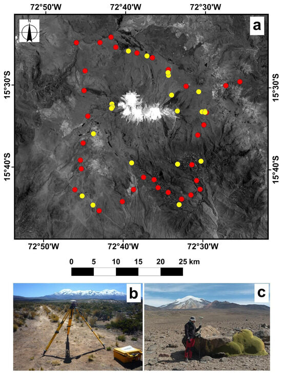
Figure 3.
(a) Distribution of orthorectification (red) and validation (yellow) points around the Nevado Coropuna icefield. (b) Measurement of control points with the Trimble R6 GNSS using the static method. (c) (left) Measurement of control points with the Leica GPS1200 using the RTK method. GPS points shown in (b,c) are located southwest and east of Nevado Coropuna, respectively.
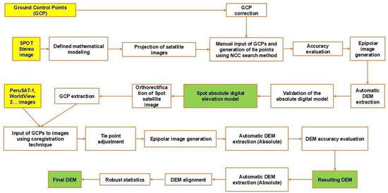
Figure 4.
Steps involved in generating high-precision DEMs.
3.5. Stereo Geometry
To analyze the geometry of the stereo images, the Base-to-height (B/H) ratio was examined, as it serves as a quality indicator for stereoscopic data in elevation extraction [27]. The optimal B/H ratio for processing 3D models through automatic correlation is 0.25 or higher, depending on the terrain. In mountainous or urban areas a high B/H ratio (greater than 0.40) improves the capture of hidden zones (e.g., between mountains and buildings) but decreases the overall automatic matching accuracy. Additionally, the convergence angle primarily affects elevation precision. Angles greater than 30° improve it, which reduces stereoscopic matching precision. The Bisector Elevation Angle (BIE) indicates the obliquity of the epipolar plane: a small BIE can degrade the accuracy of stereoscopic mapping, whereas BIEs close to 90° are considered almost orthogonal to the ground plane [28]. These parameters are detailed in Table 3.
Table 3.
Geometric parameters of stereoscopic image acquisition.
3.6. DEM Creation
Advancements in satellite-based DEM generation technology enable the rapid construction of detailed topographies, significantly improving data acquisition efficiency. These methods are more efficient and scalable than LiDAR for terrain reconstruction, because satellite images cover large areas without deployment difficulties [28]. To evaluate the accuracy and determine the mass of the Coropuna icefield, DEMs from various sensors were constructed. A stereo pair encompassing all field-collected GPS control points was selected to generate the base DEM, which served as the reference for subsequent models. The OrthoEngine module of PCI Geomatics was used to generate all DEMs, from image import to final creation.
The analysis used the fused multispectral band. Initially, the module estimated the image position using RPC metadata, generating a preliminary position. Subsequently, GCPs were manually input to improve DEM accuracy, ensuring Root Mean Square (RMS) errors below 2 m. Tie points were also generated to enhance stereo pair correlation, allowing the creation of epipolar images (left and right). This process involves matching feature points based on image overlaps and generating 3D coordinates from these points to reconstruct a stereoscopic spatial model and obtain precise 3D terrain information [29]. These reference models are essential for the orthorectification of satellite images, generating new control points to be used in subsequent DEMs for geodetic mass balance studies of glacier areas (Figure 4).
The OrthoEngine module in PCI Geomatica 2020 can read the auxiliary data provided with images in the form of Rational Polynomial Coefficients (RPCs). These RPCs define a third-order polynomial relationship between image and object space and are supplied with each image to enable transformations between image and object space. The RPC data were used to compute the coordinates of each pixel according to Equation (1). The initial orientations were corrected using GCPs to generate a 2-m resolution DEM, which reduced horizontal and vertical displacement. Tie points were then generated automatically using the Normalized Cross Correlation (NCC) method with the SUSAN approach [30]. Following RPC correction, epipolar image resampling was performed to align conjugate points in stereo images along the same image line, which in turn facilitated faster point matching [31]. After obtaining epipolars, DEM extraction was continued using OrthoEngine with the Semi-Global Matching (SGM) method at a geoid level. Medium smoothing filters were applied at a 2-m pixel resolution. The same methodology was used for all remaining models.
3.7. Precise Statistical Analysis of DEM Accuracy
Elevations are retrieved from a series of measurements, such as image grids and ground trajectories, which are related to spatial support, horizontal georeferencing, and height independence. These aspects make the concept of accuracy complex, requiring statistical analysis to estimate precision, perform model uncertainty propagation, and assess consistency. The xDEM tool [32], an open-source Python 3.9.7 package [33] for DEM analysis which includes alignment, correction, and DEM uncertainty analysis, was used to evaluate the variable vertical precision and the spatial correlation of errors that can occur at multiple spatial scales [33]. The following workflow describes the analysis performed (Figure 5).
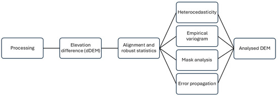
Figure 5.
dDEM accuracy analysis flow chart.
3.7.1. Robust Statistics and Alignment
To analyze the DEM statistics, the median was used instead of the mean as a robust estimator of central tendency, and the normalized median absolute deviation (NMAD) was used rather than the standard deviation as a measure of statistical dispersion. This is because both methods mitigate the effects of frequent outliers in DEMs [34]. These statistics are analyzed over stable areas by masking unstable terrain zones (e.g., glaciated areas) to ensure robustness against elevation changes from movements.
Alignment (coregistration) was performed using a reference DEM based on previously published methods [35] in combination with Deramp (Equation (3)). This method estimates horizontal translation interactively by solving a cosine equation between terrain slope, orientation, and elevation differences, while Deramp helps correct a broad category of biases (lens distortions, camera positioning) and operates quickly. This methodology was implemented using the Python xDEM package.
Aligned DEM = xdem.coreg.NuthKaab() + xdem.coreg.Deramp() + xdem.coreg.NuthKaab()
From Equation (3) a registered DEM is obtained, and coregistration statistics must be monitored and controlled as interactions progress with Equation (4) for NMAD [34].
where ~1.4826 is a scaling factor that matches the dispersion of a normal distribution, and X is the analysed sample.
NMAD(x) = 1.4826 * mediani(|Xi − median(X)|)
3.7.2. Heteroscedasticity, Spatial Correlation, and Error Propagation
DEMs have accuracy variations due to terrain and instrument-related variables. These variations in variance are called heteroscedasticity, which is rarely considered in DEM studies [31]. Elevation heteroscedasticity is estimated by sampling the empirical dispersion of elevation differences, using NMAD for N grouped categories of terrain slope [35] and curvature [31]. Once sampled, it can be modelled and applied to the spatial correlation of errors.
DEMs also present spatially correlated errors due to instrument issues or processing effects. Correlation is determined by applying non-stationary spatial statistics to estimate and model elevation error using a sum of variograms over a stable terrain, serving as an error indicator for the moving terrain (e.g., ice) [33,36]. Once heteroscedasticity and spatial error correlation are determined, they are used as the two sources for error (i.e., uncertainty) propagation. To estimate error propagation over an area of interest XDEM estimates a number of samples among the N pixels in area A that are statistically independent based on the spatial correlations (Neff) and calculates a combined standard error for the retrieved Neff, following Equation (18) cited in [33]. This approach allows for exact propagation based on the abovementioned estimated uncertainty components while maintaining computational efficiency.
3.8. Glacier Limit Delineation
All satellite imagery-based DEMs used were masked to the most extensive glacier boundary, corresponding to the year 2013. This boundary was manually delineated through interpretation of the SPOT-6 image from that year. The boundary includes the white glacier as well as areas that, based on their appearance in the satellite image, are likely either active rock glaciers or debris-covered glaciers. Active rock glaciers were identified based on characteristic features such as sets of grooves and ridges transversal to the flow or an abrupt front [37]. Debris-covered glaciers were identified as debris areas with distinctive features such as ice cliffs or supraglacial ponds [38]. The goal is to capture the full extent of glacier mass loss. Rock glaciers and debris-covered glaciers were mapped separately from the white glacier. The error associated with pixel size at the glacier boundary is considered negligible, as the pixel size in the elevation difference (dh) raster DEMs is 2 m. Ice boundaries for the 1986 and 1955 images were also manually delineated through photointerpretation, but in these cases no debris-covered ice was identified due to the lack of detail and the amount of snow cover in both cases.
3.9. Outlier Analysis and Removal for Glaciers and Gap Interpolation
When masking the unstable zone of the DEM difference for glacier mass analysis, extreme maximum and minimum values were detected in several images, which likely exist due to excessively saturated contrast areas over snow and ice [39,40]. Therefore, a normal distribution analysis was first conducted using the Shapiro–Wilk test, where the value must be less than 1 (p < 1), indicating normal behavior.
Outlier removal was performed for every temporal dh: 1955/1986, 1986/2013, 2013/2018, 2018/2020, 2020/2023 and 2023/2024. For glaciers, outlier removal cannot be simplistically applied across the entire area, but care must be taken to avoid eliminating valid values. Two ideas must be considered: first, the same positive/negative dh can be real or erroneous depending on the placement in the glacier ablation/accumulation area. For example, glaciers’ snouts tend to present negative mass balances that can reach several meters per year, especially on tropical glaciers, whereas accumulation areas show generally slightly positive values [41]. Second, despite the ice being connected among the different glaciers that compose the icefield, orientation, local topographic and even thermal conditions play a differential role among these ice masses. For example, mass loss tends to be more intense on the north face of the icecap compared to the south side, for the same elevation.
With this in consideration, the icecap was divided into 29 white (exposed ice) glaciers, based again on the photointerpretation of glacier flow forms such as crevasses or seracs in the 2013 image. Also, the debris-covered glaciers and rock glaciers were identified separately and treated as a single unit, giving a total of 30 different ice bodies (Figure 6).
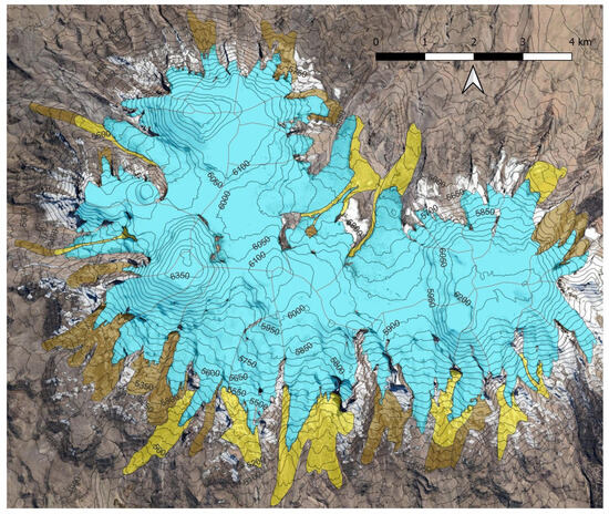
Figure 6.
Glacier delimitation in Nevado Coropuna icecap. Blue polygons correspond to white glaciers, yellow polygons to debris-covered glaciers and brown polygons to rock glaciers. The contour interval is 50 m.
The dh analysis and outlier removal was conducted on a glacier-by-glacier basis, at 50-m elevation intervals, taking the 2023 DEM as the source of absolute elevations, as it was the one featuring less potentially erroneous values. The process has two steps, implemented through the x-DEM [32] Python package: In the first step, values over or below the ±100 dh were excluded, as they are always considered unreal [42]. Second, the upper and lower outlier threshold for each difference Digital Elevation Model (dhDEM) was defined as those falling out of ±1 standard deviation (STD) of all the valid values in the altitudinal belt. This is a more cautious threshold than the suggested in the literature [35] but was chosen in order to make sure that most of the erroneous values were actually removed. In addition, the comparison between the 1955 and 1986 image showed a consistent positive dh on the NW section of the icecap, which was interpreted as an error on the contour delineation for the 1955 image. This led to the complete removal of this part of the icecap, which was not considered for the 1955–1986 dh analysis. Using this method, a variable percentage of glacier surface was eliminated in all cases. The resulting dhDEMs were filled using a local hypsometric interpolation [35], which fills the gaps with the average the value of the elevation belt in which the gap is located. This procedure was applied on a glacier-by-glacier basis in a similar method to the outlier removal and using the xDEM library [32].
3.10. Glacier Mass Balance
Volume calculations for Nevado Coropuna were performed using the polygon generated in 2013 as the baseline for deglaciation analysis. The glacier volume change at each point corresponds to the elevation change between two DEMs. The total volume change is obtained by summing all values and multiplying by the pixel area.
To calculate the mass balance, the ice volume change was multiplied by 0.85 with a 0.06 uncertainty added, considering that the ice density was set at 850 ± 60 kg/m3. This density is recommended for periods longer than five years, with stable mass balance gradients, the presence of a firn area, and significant volume changes [43]. Finally, volume statistics, including standard deviation, mean, and 95% confidence interval were calculated per year, dividing the result of each dhDEM by the elapsed years.
4. Results
4.1. Reference DEM (DEMref) Quality Assessment
All the resulting DEMs can be found in Zenodo (https://zenodo.org/records/16419040). The reference DEM (Figure 7) and the base image are essential data for building elevation models. To ensure their reliability, the vertical and horizontal accuracy was evaluated using the 19 validation points distributed across the study area (Figure 3a). As shown in Table 4, a vertical RMSE of 1.50 m was obtained, with a 95% confidence accuracy of 3.02 m. This value fits within the standards of the IGN: vertical RMSE ranging between 6.25 m and 12.5 m at 95% confidence. Regarding the horizontal accuracy of the orthorectified images, the RMSE was 0.72 m in Easting and 0.97 m in Northing, with 95% confidence intervals of 1.25 m (East) and 1.68 m (North). IGN standards require a horizontal RMSE of 4.24 m and 7.33 m at 95% confidence for 1:25,000 scales, so these values also comply with IGN standards. The mean values of the three dimensions in Table 2 indicate a systematic shift in the DEM and orthorectification, with a Z offset of 0.54 m, suggesting a slight overestimation of elevation, and horizontal offsets of 0.52 m East and 0.40 m North, showing a small displacement from the ground control points. The RMSE of 1.51 m in Z implies a moderate height estimation error, which is common in DEMs derived from satellite imagery [36]. In the horizontal component, values of 0.77 m (East) and 0.83 m (North) show low uncertainty.
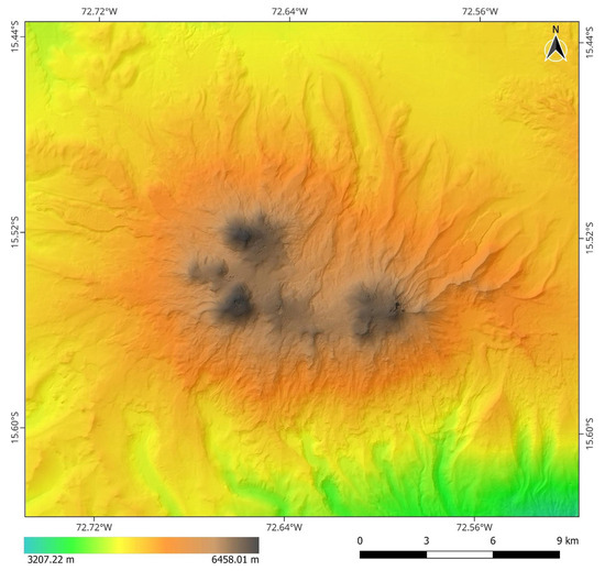
Figure 7.
Resulting base DEM.
Table 4.
Three-dimensional BaseDEM error assessment.
Table 5 suggests that all the DEMs are very similar in terms of the mean and absolute values, with the exception of the maximum value, which has a wide range. This difference points to potential errors in the highest areas of the icefield. Table 6 presents the evaluation of the elevation differences between each DEM and the reference, including unstable areas (glaciated zones), using the SPOT 2018 DEM as a reference. The comparison was conducted using basic descriptive statistics: mean, median, and standard deviation. The models based on aerial images (AERIAL 1955 and AERIAL 1986), exhibited the largest absolute elevation differences. The 1955 DEM presented a mean difference of −6.93 m, with a maximum of 110.10 m and a standard deviation of 0.83 m, suggesting a considerable altitudinal bias. Similarly, AERIAL 1986 yielded a mean of −6.64 m, a median of −15.26 m, and a standard deviation of 0.83 m. These results are attributed to the models’ analysis of both stable and unstable (glacier) zones, and to the 31-year temporal gap with respect to the reference DEM, which contributed to these anomalies.
Table 5.
Basic statistics for the used DEMs.
Table 6.
Difference between resulting DEMs and the BaseDEM.
In contrast, more recent digital models showed significantly smaller differences. PERUSAT-1 2023 presented a mean of −0.60 m, a median of 0.36 m, and a standard deviation of 0.67 m, while Pléiades 2024 was the most consistent with the reference DEM, with a mean of 1.18 m, a median of 0.35 m, and a standard deviation of just 0.64 m. The SPOT 2013 and WorldView (WV) 2020 models showed mean differences close to zero (−0.15 m and 0.18 m, respectively), although with broader extreme values, indicating possible local displacements or errors associated with terrain characteristics and acquisition conditions. Overall, there is a noticeable trend of improved altimetric consistency in the more recent DEMs. This could be attributed to higher spatial resolution, better stereoscopic correlation algorithms and reduced systematic noise.
An analysis of the median and standard deviation of the DEMs reveals a strong alignment, and therefore also good consistency among the different datasets. The median differences are all below approximately 1.30 m for DEMs obtained between 2013 and 2024, which represents terrains with similar average elevation characteristics. The standard deviations of the four mentioned models are also close, showing similar variability in elevation. This suggests that data dispersion is comparable across sensors.
4.2. DEM Visual Evaluation and Histogram Analysis
Figure 8 shows the elevation distribution of the seven DEMs using density curves, allowing comparison and detection of distribution discrepancies. All curves overlap across the elevation range of 4750 m to 6500 m, suggesting consistent topographic capture. Density peaks are observed around 5000–5300 m and 5500–6000 m, likely corresponding to dominant topographic features of Nevado Coropuna. Above 6000 m, density drops sharply, indicating fewer high-elevation areas. No significant deviations are observed among the satellite-based DEMs, suggesting consistent generation methods and results. However, quite significant variations can be found in the 1986 and 1955 images. The differences are located from 5100 m upwards, which correspond to the ice cap area, so they are not systematic to the DEM reconstruction process, but specific to problems on the ice-covered area.
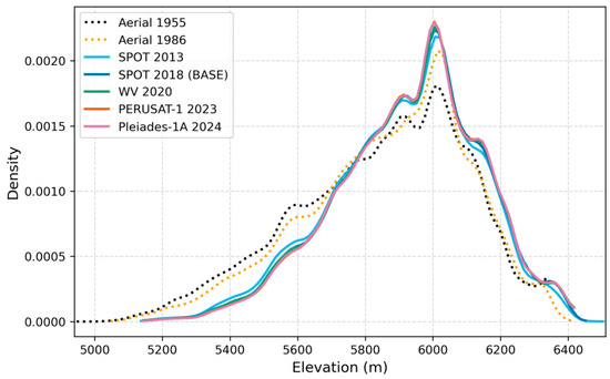
Figure 8.
Density elevation distribution curves of the different DEMs in Nevado Coropuna.
A visual analysis of DEM discrepancies can be found in Figure 9, which shows a ~20 km longitudinal elevation profile drawn across Nevado Coropuna (NW to NE, see Figure 9a). The profile crosses diverse slopes and terrain shapes, revealing model consistency under varying topographic conditions, but it also confirms the presence of errors. The 1955 DEM shows errors mostly derived from the TIN interpolation from contours, which create unrealistic, sharp-edged profiles. The 1986 DEM shows some unrealistic distortions in the first peak area and consistently low values between kms 7 and 8, although the rest of the profile successfully matches the other DEMs. The 2013 DEM presents high noise in peak areas, a fact which is also noticeable, albeit to a lesser extent, in the 2018 DEM. From 2018 onward, DEMs show high correspondence with minimal elevation differences, suggesting an improved data quality, which supports data reliability and insights into glacier or terrain surface changes.
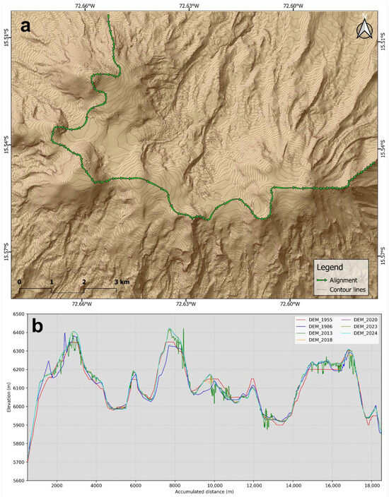
Figure 9.
(a) Track along the peaks in Nevado Coropuna. (b) Profile along track for the different DEMs.
Errors found in Spot-6 2013 and 2018 data probably stem from image brightness saturation, which is common in snow-covered zones and creates excessive noise and elevation overestimation [35]. This possibility can be checked on Figure 10 from SPOT 2013 and 2018 images, in which high brightness surfaces at the icecap accumulation area can be identified.
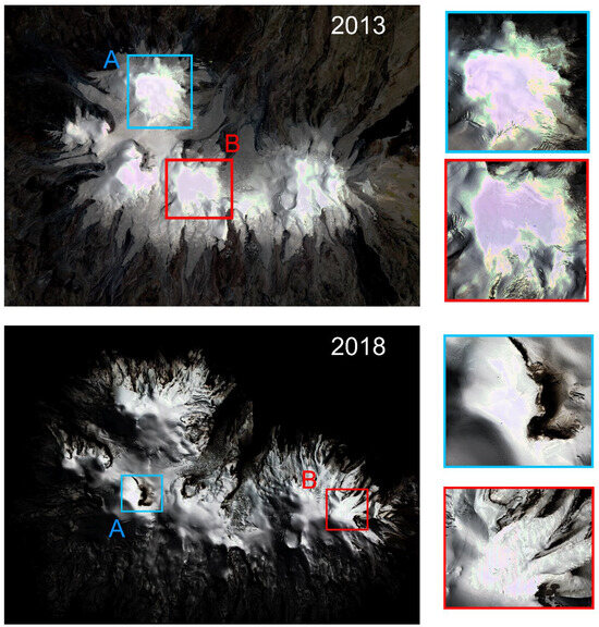
Figure 10.
Errors in image acquisition for the SPOT 6 (2013) and SPOT 6 (2018). A and B highlight anomalies causing DEM errors.
4.3. Difference Analysis and DEM Correlation
Table 7 evaluates DEM accuracy before and after the coregistration process, based on elevation differences and horizontal pixel shifts. For each DEM difference pair, three main statistical metrics were analysed: NMAD (Normalized Median Absolute Deviation), RMSE (Root Mean Square Error), and LE90/CE90 (Linear/Circular Error at 90% confidence). Before coregistration the highest NMAD values were observed in pairs involving historical aerial imagery (Aerial 1986 and 1955). For instance, the SPOT (2018)—Aerial (1986) pair shows an NMAD of 5.99 m, while the SPOT (2018)—Aerial (1955) pair reaches up to 15.728 m. These values reflect high vertical dispersion and, therefore, lower altimetric precision.
Table 7.
DEM differences before and after alignment.
Horizontal accuracy was initially low, with CE90 (Circular Error at 90% confidence) and LE90 (Linear Error at 90% confidence) values ranging from 58.912 m to 186.40 m and RMSE values from 27.452 m to 86.859 m. These figures indicate poor spatial correspondence between models and inconsistencies in alignment. DEM pairs based on modern imagery exhibit significantly improved accuracy. NMAD values range from 1.7 m to 1.793 m, indicating low vertical variability. Regarding horizontal accuracy, CE90 values range from 4.786 m to 9.191 m, with RMSE values between 2.230 m and 4.283 m, suggesting only minor alignment inconsistencies compared to historical image pairs.
Following coregistration, NMAD values decreased significantly, especially for modern DEM pairs, with values below 1.5 m—suitable for glacier studies and detailed elevation analyses. Horizontal RMSE values also dropped notably, falling below 1 m in recent DEM pairs. This indicates a very good positional fit, suitable for reliable multitemporal analysis. Despite this geometric correction, some pairs still exhibit significant limitations. The SPOT 6 (2018)—Aerial (1955) pair maintains high NMAD and RMSE values, reflecting the challenges of integrating historical datasets with modern sensors. This may limit their use in precise quantitative studies, particularly in steep or glacially dynamic areas. The SPOT (2018)—Aerial (1986) pair shows better accuracy compared to the 1955 pair but still presents considerable errors. It is therefore more appropriate for qualitative analysis or identifying general trends but should be used cautiously in applications requiring sub-meter accuracy.
The SPOT 2018—Aerial 1955 pair exhibited the highest horizontal RMSE of 86.8 m, indicating a significant displacement. As more recent data are considered, errors decrease sharply, thanks to the improved absolute positioning of modern sensors. Coregistration substantially reduced horizontal errors across all DEM pairs, particularly for the oldest ones. The SPOT 6 (2018)—Aerial (1955) pair decreased to 19 m and the SPOT 6 (2018)—Aerial (1986) pair dropped to 3.4 m. For the most recent pairs (SPOT6, WV1, PHR1A, PER1), the initial RMSE was already low, but coregistration further improved the alignment, reaching values close to or below 1 m. These improvements highlight the enhanced quality of the models and their suitability for future multitemporal change detection and other high-precision applications.
Figure S1 in Supplementary Materials shows the elevation difference maps obtained by comparing the reference DEM from SPOT 6 (2018) with the other models. Significant elevation differences were observed prior to adjustment in the oldest DEMs (Aerial 1955 and Aerial 1986). These discrepancies reveal the presence of systematic errors, likely due to poor georeferencing or inaccuracies inherent to the method. The coregistration process considerably reduced these differences, especially in stable terrain, which improved the geometric consistency. This is particularly evident in recent DEMs (SPOT 2013, WV1 2020, PERUSAT-1 2023, and PHR1A 2024).
As expected, some of the elevation changes persist after this correction, suggesting that they are not geometric errors, but real topographic changes associated with glacier dynamics. Overall, the results demonstrate that geometric coregistration is essential for correcting systematic errors, especially in DEM pairs with wide temporal gaps [35].
4.4. Data Quality Assessment: Heterocedasticity, Spatial Correlation and Error Propagation
Figure S2 in Supplementary Materials shows the error assessment for all the dhDEMs. The standardized elevation change maps show z-score normalized elevation changes (glacier area is masked). Blue/red tones indicate significant positive/negative changes in standard deviation units. Most areas fall within the [−3, 3] range, suggesting changes are statistically reasonable and within an acceptable threshold.
Density plots show how vertical error (NMAD) varies with slope and curvature. NMAD increases in steep areas (>30°) but is less sensitive to changes in curvature, although an increase in error is found in spots with low slope but high curvature.
The 1955–1986 and 1986–2013 DEMs show a very clustered distribution in terms of curvature and errors concentrated in zero curvature areas for the 1986–2013 DEM. Overall, there is a heteroscedastic error behavior—error increases in complex terrain. The empirical variogram shows the spatial autocorrelation of elevation differences. At short distances (<100 m), variance increases rapidly, suggesting structured noise or spatially correlated errors. The fitted curve (orange), combining spherical and Gaussian models, is used for subsequent error propagation. Curve stabilization at long distances indicates loss of correlation, as expected in random errors.
The error propagation map shows the propagated uncertainty between dhDEMs, which has been used to convert elevation changes into volume/mass variations with reliable uncertainty estimates [43]. During the 1986–1955 period, a high standard error of ±5.30 m was observed, albeit distributed over a long-time span. However, significant uncertainty is associated with the quality of historical photogrammetric data, which presents vertical errors stemming from the technological limitations in the generation of DEMs from old images. In contrast, between 1986 and 2013, a significant elevation loss and low error indicate a clear glacier loss. The magnitude of this change far exceeds the margin of uncertainty, which confirms the robustness of our findings.
More recent periods (2013–2018: 0.29 m ± 0.35 m, and 2018–2020: −0.14 m ± 0.17 m) show changes within the uncertainty range, although it is important to note that some of these data feature obvious outliers that were subsequently filtered out (see Section 4.5). Between 2020 and 2023, an elevation loss of −1.83 m ± 0.19 m is observed, which is statistically significant. Finally, the 2023–2024 interval shows a change of −0.17 m ± 0.28 m, which again falls within the uncertainty.
Across the 1986–2013, 2013–2018, 2018–2020, 2020–2023 and 2023–2024 periods, precision improves, which can be attributed to the use of high-resolution satellite optical sensor data and more robust geometric correction processes. These advances allow for the minimization of both systematic and random errors. In general, the error values obtained are consistent with similar studies conducted in tropical glacier environments. Our results confirm that the most recent DEMs offer the necessary reliability for detecting glacier elevation changes, whereas pre-existing data present limitations that must be considered when interpreting them.
4.5. Outlier Removal and Gap Interpolation
Outlier removal resulted in the elimination of a significant part of the dhDEMs. Data elimination was more extensive in the dhDEMs that were derived from the 1955 and 1986 aerial images (Table 8). A visual assessment of the deleted areas reveals a uniform outlier removal, except in areas where obvious errors had been identified, especially at the accumulation area of the icecap in the 1986, 2013 and 2018 DEMs.
Table 8.
Percentage of the dhDEMs eliminated for each interval.
Table 9 shows that the results of the local filling interpolation results for the entire glacier are consistent very close to the values obtained without interpolation, confirming that local interpolation will not introduce artifacts to the final mass balance.
Table 9.
Average elevation difference (dh yr−1) in dhDEMs after outlier removal.
4.6. Total Mass Balance
According to Table 10, we have estimated that Nevado Coropuna has lost 34.24 ± 2.2 Hm3 in the white glaciers and 11.74 ± 0.84 Hm3 on debris-covered and rock glaciers for the 2013–2024 timeframe. This corresponds to 1.52% of the total estimated ice-stored water resources in the area. Between 1955 and 2013 the mass loss was 149.63 ± 16.08 Hm3, but this figure is lower than the real mass loss, because the NW section of the icecap was not considered for the 1955–1986 interval and the rock glacier mass loss was not accounted for either.
Table 10.
Mass balance in w.e. for the different timeframes. Uncertainty accounts for the DEM difference error propagation and the uncertainty inherent from ice/water transformation in the case of white glaciers, and only for the DEM-related error propagation in the debris-covered ice.
4.7. Mass Balance per Elevation and Timeframe
Detailed mass balance maps can be calculated from Zenodo (https://zenodo.org/records/16419040). Figure 11 shows the evolution of dh yr−1 per elevation on the white glacier and debris-covered glacier from 2013 to 2024. The dh in the 1955–1986 timeframe is only slightly negative until the 5700 m contour, where dh transitions to positive values, but always within the 1 STD limit. There is a clear evolution to much larger yearly negative mass balances in the 1986–2013 timeframe, while the 0 dh threshold also moved upwards on the glacier to the 6050 contour. The very positive dh in the plots for the 2013 and 2018 DEMs must be taken with caution, because they might mean that there are still artifacts not removed as outliers. In any case, they affect only a minimal part of the glacier, above 6250 m. The negative trend in 1986–2013 is kept during the following years. The 2013–2018 dh trend is very similar to the previous one and the 2018–2020 period shows even deeper mass loss in the glacier snouts reaching nearly 4 m of ice loss every year. The 2020–2023 trend is the most worrying one, because it shows a general ice downwasting, even at the highest part of the icecap. The plot for 2023–2024 keeps the same trend as before 2020, but it must be considered with caution, because of the amount of snow present in the 2024 image. In summary, plots show an accelerating mass loss in the glacier’s lowest areas and a general glacier thickness decrease even in the accumulation area. Finally, the plot for the debris-covered glacier also shows a generally negative dh, but with a less steep negative trend at similar and lower elevations, compared to the white glacier.
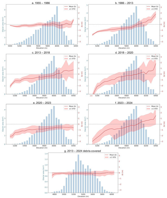
Figure 11.
Plots show dh per altitudinal interval between 1955 and 2024. (a). dh 1955–1986. (b). dh 1986–2013. (c). dh 2013–2018. (d). dh 2018–2020. (e). dh 2020–2023. (f). dh. 2023–2024. (g). dh. 2013–2024 in debris-covered and rock glaciers.
4.8. Mass Balance per Glacier
The distribution of mass balance across the different outlets of the Nevado Coropuna icefield (Figure 12) shows that ice loss is present across all the orientations and timeframes, highlighting deglaciation as an overall trend in the glacier. However, there is an enhanced deglaciation in the central-northern sectors, which drain the largest areas in the top of the ice plateau. Deglaciation is even more pronounced in the northeast glaciers. Conversely, deglaciation is less intense at the west and northwest glaciers. Southern oriented outlets show a not so uniform behaviour, southwest glaciers, which are the ones that reach the lowest elevations, seem to be the most affected by deglaciation, while southeastern outlets seem to exhibit greater resilience. Debris-covered and rock glaciers show a generally weak deglaciation pattern. Only three debris-covered glaciers, placed in different sectors of the icefield, show a clear deglaciation pattern.
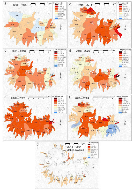
Figure 12.
Annual dh in meters per glacier in Nevado Coropuna icefield. (a). 1955–1986. (b). 1986–2013. (c). 2013–2018. (d). 2018–2020. (e). 2020–2023. (f). 2023–2024. (g). 2013–2024 in debris-covered and rock glaciers.
5. Discussion
5.1. Sources of Error and Data Reliability
The implementation of the procedures following [32,33] improved the resulting DEMs. The errors in dh are well below the glacier evolution signal, so the data can be considered to reflect real changes in the ice. The local hypsometric interpolation method used for filling the voids generated by the outlier-removal procedure has proved to best maintain the elevation difference when compared to the unfiltered data. The difference is ≤0.01 m in all cases, in accordance with [44].
The data quality for the satellite DEMs remains sufficient in all cases. However, the data acquired from the photogrammetric reconstruction of the 1955 and 1986 imagery exhibits a lower resolution, poorer quality and obvious errors in extensive areas, which makes a noticeable part of the icefield unusable. This data, however, presents a high importance for the ice mass balance trend reconstruction, which is the reason it is kept. Moreover, the large NMAD in the dhDEMs that use the aerial-image retrieved DEM (±5.3 m for 1955–1986 and ±0.59 for 1986–2013) is offset by the large temporal lapse between the aerial images and the satellite imagery. It is worth highlighting the quality of the data provided by the PeruSat-1 satellite, which shows error levels comparable to those of other satellites (SPOT, Pleiades, WorldView) more widely used in geodetic mass balance calculations [45,46].
5.2. Results Comparison with Other Glacier Mass Balance Works
Glacier thinning shows a worldwide accelerated trend, with very minor exceptions in polar and subpolar areas [47]. Those authors estimated that the annual average mass loss in tropical glaciers is −0.5 ± 0.2 m. water equivalent (w.e.) yr−1. Results from [48] in the Vilcanota Range, on the southeastern (humid) edge of the Peruvian Altiplano show a −0.48 ± 0.07 m.w.e. yr−1 rate for the 2000–2020 timeframe, with a linear, not accelerating, deglaciation trend.
Ref. [49] calculated a decreasing deglaciation between 2000 and 2016, with a −0.52 ± 0.11 m.w.e. yr−1 mass balance for the 2000–2016 timeframe but a −0.05 ± 0.09 m.w.e. yr−1 between 2013 and 2016 in the Ampato region, where the largest glaciated area corresponds to Nevado Coropuna. On the other hand, ref. [50] calculated a mean surface lowering of −0.2 ± 0.3 m.w.e. yr−1 in Nevado Coropuna for the period between 1955 and 2002. Both findings suggest an accelerating deglaciation trend since the onset of the XXI century. If we consider mass balance studies further South, in the Dry Andes region [51], they pointed to a mass balance average of −0.28 ± 0.18 m.w.e. yr−1 for the entire region between 2000 and 2018, and other authors measured a −0.24 ± 0.10 m.w.e. yr−1 mass balance in the Tapado glacier (La Laguna catchment, northern Chile) between 2000 and 2020 [10].
Our results show an average mass loss on the Nevado Coropuna glacier system of −0.36 ± 0.12 m.w.e. yr−1 for the 2013–2024 period, which is slightly lower than the average reported for the humid Tropical Andes by [47] and aligns more closely with values for the Dry Andes further south and even on the Northern Patagonian Icefield [51]. This finding is likely a result of Nevado Coropuna’s location in a transitional climatic zone. While glaciers in the moister, eastern Cordilleras of Peru (e.g., Vilcanota, [48,49]) are influenced by a stronger influx of moisture from the Amazon basin, Coropuna’s position on the western, arid flank and its broad, high-elevation plateau, which promotes snow retention, likely contributes to an overall mass loss more similar to the Dry Andes, located further south.
Notwithstanding this difference with the general trend of the tropical glaciers, mass loss was limited between 2013 and 2018 (−0.27 ± 0.07 m.w.e. yr−1) but has since then accelerated to a rate comparable to the tropical glacier average (−0.43 ± 0.12 m.w.e. yr−1 [47]).
The recent acceleration contrasts with the overall stable rate of mass loss observed in the Vilcanota Range [48]. This suggests that the Coropuna icefield is now responding more significantly to regional climatic shifts, a trend also noted by prior research for other Peruvian glaciers in the humid outer tropics, particularly between 2013 and 2016 [49]. The low mass loss between 2023 and 2024 is probably due to the heavy snowfall in the wet season of 2024, so there is a seasonality imprint which is not related to ice loss.
During the last studied year the mass balance trend remained negative but less pronounced. However, this last value does not take into account an abnormally wet and cold season in 2024. Even though glacier retreat in terms of area is less severe in Nevado Coropuna than in glaciers at the eastern (wet) border of the Andean Altiplano in South Peru [16,52], mass balance is similar, meaning that ice loss at the snouts is being balanced out by glacier thinning.
The average yearly mass balance for the debris-covered and rock glaciers for the 2013–2024 season is −0.09 m.w.e. yr−1, which is four times less rapid than the white glaciers, despite being predominantly located at lower elevations. Average mass balance in debris-covered glaciers for Cordillera Blanca was measured by earlier studies [53] in −0.7 m. for the 2014–2015 year and, more similarly to Nevado Coropuna, mass balance in rock glaciers at the dry Andes was measured at to −0.440 ± 0.11m yr−1 for the debris-covered section of the glacier and +0.08 ± 0.11m yr−1 for the rock glacier section between 2012 and 2020 [10], but they acknowledge that some rock glaciers might have run out of ice, being that the reason for not thinning, with the alternative of a complete debris insulation that prevents ice loss. This might also be the case in Nevado Coropuna, and a further study on velocities and geophysical surveys at the debris-covered and rock glacier would help find ice content and activity of ice-cored areas.
Before 2013 two phases can be distinguished from the Coropuna data: 1955 to 1986 the mass balance was near stability, but ice loss accelerated in the 1986–2013 timeframe. Other contributions from semi-arid regions in Chile [10,54] also point at a nearly stable mass balance between the 1950s and the end of the XX century. Further investigation on this timeframe should bring light to the moment when ice loss commenced at Nevado Coropuna.
5.3. Local Distribution of the Measured Mass Balance in Nevado Coropuna
5.3.1. Mass Balance per Altitudinal Belt and Glacier Type
The altitudinal distribution of average geodetic mass balance shows an accelerating mass loss in the glacier’s lowest areas and a general glacier thickness decrease. The observed thinning in the ice mass extends worryingly to the areas closest to the summits of Nevado Coropuna, as the 2020–2023 data points out. This fact is not only noted by dh data in different altitudinal bands but also evidenced by the appearance since 2013 of new ice-free zones, even at the icecap’s top. Figure 13 shows the example of the southwestern peak, which is the highest and the most ascended by mountaineers. The image sequence shows how an ice-free area opened between 2013 and 2018 at the east of the crater, and the ice around has remained with negative dh since then. Due to their lower albedo, these bedrock exposed surfaces work as hotspots that enhance melt and sublimation, creating a vicious circle of mass loss. The figure also shows how ice is thinning at the margins of the crater, especially on its northwest side.
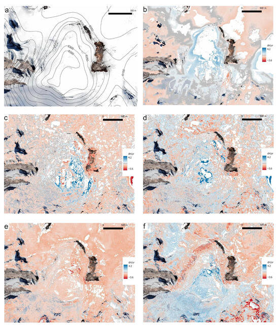
Figure 13.
Images show dh at the southwestern peak and crater area. (a). Image from Google Satellite. (b). dh 1986–2013. (c). dh 2013–2018. (d). dh 2018–2020. (e). dh 2020–2023. (f). dh 2023–2024. White areas correspond to pixels whose values were considered outliers according to the methods explained in Section 3.9.
At the same time, mass loss at glaciers’ snouts has also accelerated from few centimeters of annual dh in the 1955–1986 data to around 3 m of annual ice loss since 2020, but it is consistently below −2 m·yr−1 since the 2018 image, with a marked negative peak in the 2018–2020 timeframe. Figure 14 shows that the mass loss trend in the lowest parts of the icefield is up to 10 times stronger than in the highest parts. In fact, the mass loss trend is significant up until the 6000 m elevation, but not further up.
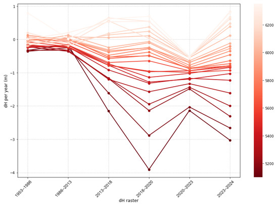
Figure 14.
Evolution of annual dh at different elevation belts. Note that the horizontal axis is temporal, but not to scale.
Accelerated ice melt in the ablation area, led by temperature increase (as opposed to sublimation), might also trigger glacier velocity changes, which will contribute to enhanced mass loss, because more ice will be conveyed downslope. This behaviour has been described in the Cordillera Blanca and even related to ENSO events [55]. Again, a further investigation on ice velocities (e.g., analysing radar images) would confirm this hypothesis.
Debris-covered glaciers and rock glaciers are important and extensive features around Nevado Coropuna, with 23% of the total glaciated area in 2013, according to our limits mapping. Mass balance in debris-covered areas accounts, however, for 6.5–7% of the total mass loss in most cases, except the 2023–2024 season, in which the dh is positive for these areas. The behaviour of debris-covered ice differs from the accelerating trend mentioned, with a slightly negative dh which is nevertheless not uniform, but more clearly negative around supraglacial ponds and ice cliffs in debris-covered glaciers, and almost even in rock glaciers (see Figure 15). This trend is like examples elsewhere in South America [10,53] or the Himalayas [56]. This result points out the importance of buried frozen water as a long-lasting resource in the current context of warming climate. This idea is even more powerful if we consider that deglaciation will likely enhance rockfall and other events related to slope instability, potentially extending the debris-covered glacier and rock glacier areas, in the near future.
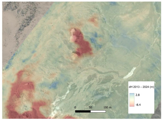
Figure 15.
Image shows dh contrast in a debris-covered glacier of the northern face of the Nevado Coropuna. Mass loss is concentrated on ice cliffs around supraglacial lakes.
The observed trends suggest a future icecap evolution towards the fragmentation into smaller glacier units, which would have negative implications for ice conservation: it would increase the surface area exposed to solar radiation and, consequently, increase the vulnerability of glaciers to the impact of climate change. This is a crucial aspect for projecting the future of the glacier system in a climate change scenario.
5.3.2. Contrasts in Glacier Evolution Between Outlets
The elevation averaged values hide variations between the north and south outlets. Eight out of the ten glaciers that accumulated a higher average mass loss between 2013 and 2024 are located at the northern half of the icefield. The three central northern glaciers are the ones that accumulated most of the mass loss, as they drain the central area and part of the western and eastern high crater areas. The central area is the lowest peak area, comprising the locally called “saddle”, an area below 6000 m that is undergoing an accelerated mass loss. Because Nevado Coropuna is an active volcano, there is another important factor in ice ablation: geothermal heat [18]. The available data in [18] reveals an uneven distribution of geothermal heat. In the eastern sectors of the volcanic complex, continuous ground temperature records show higher elevations (~5600 m) with long periods without freezing [18], while permafrost exists at lower altitudes (~5000 m: [13]). Likewise, the highest accumulated mass loss corresponds to the northeasternmost glaciers, which are located in the mentioned active volcanic area, where the last eruptions happened 1–2 ka ago [18,19]. On the other hand, southeastern and western glaciers have undergone a much lower mass loss. Southeastern glaciers are best oriented for snow preservation, and they drain very high accumulation areas from the eastern craters. Meanwhile, low ice loss on the northwest might be due to a lower geothermal gradient in the area, although this idea is not backed by any data. Further observations of air and ground temperatures around Nevado Coropuna are required to understand ice response to the rhythms of external climate and endogenous heat.
5.4. Mass Balance and Climate: The Effect of ENSO Events
ENSO events affect Peruvian glacier mass balance [8]. Positive ENSO will entail an enhanced negative mass balance due to temperature increase and precipitation reduction, whereas negative ENSO phases have the opposite effect, thanks to enhanced precipitation and lower temperatures. However, while ENSO events lead to significant interannual variability of Andean glaciers’ energy and mass balance, the long-term negative trend cannot be pinned on tropical Pacific Sea surface temperatures [57]. According to [58], the retreat has accelerated over the past three decades, with an average mass loss in the tropical Andes estimated at −0.76 m w.e. over the period 1976–2010. The annual dh evolution shown by our data is not sufficiently resolved until 2013, although an acceleration is clearly visible after 1986. Since 2013, dh does not follow a trend related to ENSO events (Figure 16), but seems relatively independent of them, with an overall negative mass loss acceleration during the 2020–2023 La Niña ENSO event. Given the size of the Coropuna icefield, it can be inferred that it does not react to short term events like ENSO, unlike observations on smaller glaciers such as Shallap in Cordillera Blanca [59]. It must be stressed that, even if the ENSO events can be traced in the glaciological mass balance and annual ELA, the annual dh is also the result of ice flow, in which long-term dynamics plays a role. However, if we only consider the mass loss variability at the lowest parts of the glaciers (below 5500 m), they do follow the ENSO oscillations during the 2013–2024 timeframe. A comparison of mass balance to measured precipitation and temperatures in the area will bring a better understanding of the response of the Coropuna icefield to climate trends and shifts.
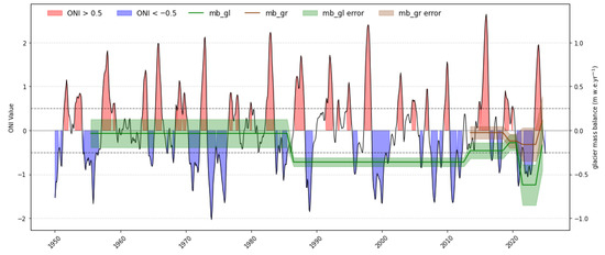
Figure 16.
Nevado Coropuna mass balance and ENSO. Source of ENSO Oceanic Niño Index (ONI) data: https://psl.noaa.gov/data/correlation/oni.data (accessed on 1 July 2025).
6. Conclusions
This study successfully combined photogrammetric aerial imagery and satellite images to assess the mass balance of the world’s largest tropical icefield, spanning 69 years (1955–2024). PeruSAT-1 satellite imagery was employed for the first time in geodetic mass balance calculations and provided quality results comparable to other satellites commonly used in similar research applications, such as Pléiades or SPOT-6.
While results derived from earlier photogrammetric data exhibit lower consistency, they extend the observational period back to the mid-20th century. This data indicates that the Coropuna icefield remained largely stable between 1955 and 1986 with −0.04 m dh yr−1. Ice decline has accelerated since then to a maximum annual dh yr−1 of −0.73 ± 0.19 in the 2020–2023 timeframe. No consistent relationship between mass loss and ENSO cycles was found, suggesting that the icefield’s substantial size buffers short-term climatic cycles.
The average mass loss (−0.36 ± 0.12 m.w.e. yr−1 for the 2013 to 2024 period) is greater than in other glaciers in the Arid Andes of Chile or Argentina, but similar or slightly lower than that observed in other glaciers located in the moister Peruvian Andes. This finding suggests that Nevado Coropuna lies in a transition zone between both climatic environments.
Mass loss in the Coropuna glacier system is spatially heterogeneous. The highest rates of loss, with annual dh averages between −1 and −1.5 m. occur in the northern glaciers, especially in the northeast. This northern concentration of loss may stem from the higher insolation exposure. However, the pronounced loss in the northeast also aligns with the geothermal activity in the area where recent eruptions have taken place. In contrast, glaciers in the southwestern sector have remained comparatively more stable, with annual dh averages between 0.15 and −0.76 m. Debris-covered glaciers and rock glaciers exhibit significantly less mass loss: the reduction is concentrated in a few surface areas, especially on ice cliffs and supraglacial ponds.
Finally, it is extremely worrying to observe that the descent of the ice surface extends to the summit areas, because it suggests that in the coming decades a continuous process of fragmentation of the icefield into smaller glacier units will occur, which will make the remaining ice even more sensitive to climate change.
Supplementary Materials
The following supporting information can be downloaded at: https://www.mdpi.com/article/10.3390/rs17193344/s1, Figure S1: Elevation difference maps pre- and post-alignment. Figure S2: Data quality assessment of DEMs based on stable areas, showing different statistics that validate the results. The following datasets used in this study are publicly available: https://zenodo.org/records/16419040.
Author Contributions
Conceptualization, R.P. and J.Ú.; methodology, J.L., R.P., A.D.J.A.-G. and J.Ú.; software, J.L., R.P., A.D.J.A.-G. and J.Ú.; validation, R.P., J.Ú. and A.D.J.A.-G. formal analysis, J.Ú. and R.P.; investigation, J.Ú., R.P. and J.P.; resources, J.P., J.Ú., R.P.; data curation, J.L., A.D.J.A.-G.; writing—original draft preparation, R.P., J.Ú., J.L.; writing—review and editing, J.L., R.P. and J.Ú.; visualization, J.L., R.P. and J.Ú.; supervision, J.L., R.P., J.Ú. and A.D.J.A.-G.; project administration, J.Ú., R.P. and J.P.; funding acquisition, R.P., J.Ú. and J.P. All authors have read and agreed to the published version of the manuscript.
Funding
This research was funded by the following grants: Ministerio de Ciencia, Innovación y Universidades de España: PID2020-113247RA-C22; Universidad Nacional de Educación a Distancia (UNED) Talento Joven: 2021V/-TAJOV/005.
Data Availability Statement
Digital Elevation Model (DEM) datas can be found in Zenodo (https://zenodo.org/records/16419040).
Acknowledgments
This work was funded by the Ministerio de Ciencia e Innovación of Spain through the research project (PID2020-113247RA-C22) and the Universidad Nacional de Educación a Distancia (UNED) Talento Joven grant 2021V/-TAJOV/005. It was also made possible thanks to the ONG Guías de Espeleología y Montaña (GEM) and Canal de Isabel II (Madrid’s public water utility). The authors also wish to thank Jesús Quintana (CONIDA) for the initial laboratory work, to Luis Calle and Justo Girón (CONIDA), and Álvaro Arredondo and Pablo Guijarro (GEM) for their significant efforts during the fieldwork. The authors particularly acknowledge Silvio Arias (Ex-Consejero Regional de la Provincia de Castilla, Arequipa), whose crucial support in arranging transportation and accommodation was indispensable for the entire expedition. Finally, the authors thank Romain Hugonnet (University of Washington) and Etienne Berthier (LEGOS, Toulouse) for their valuable help. Reviewers are thanked for their positive and useful comments.
Conflicts of Interest
The authors declare no conflict of interest.
References
- Nogués-Bravo, D.; Araújo, M.B.; Errea, M.P.; Martínez-Rica, J.P. Exposure of global mountain systems to climate warming during the 21st Century. Glob. Environ. Change 2007, 17, 420–428. [Google Scholar] [CrossRef]
- Viviroli, D.; Dürr, H.H.; Messerli, B.; Meybeck, M.; Weingartner, R. Mountains of the world, water towers for humanity: Typology, mapping, and global significance. Water Resour. Res. 2007, 43, 1–13. [Google Scholar] [CrossRef]
- Urrutia, R.; Vuille, M. Climate change projections for the tropical Andes using a regional climate model: Temperature and precipitation simulations for the end of the 21st century. J. Geophys. Res. Atmos. 2009, 114, 1–15. [Google Scholar] [CrossRef]
- Garreaud, R.D. The Andes climate and weather. Adv. Geosci. 2009, 22, 3–11. [Google Scholar] [CrossRef]
- Lejeune, Y.; Bouilloud, L.; Etchevers, P.; Wagnon, P.; Chevallier, P.; Sicart, J.-E.; Martin, E.; Habets, F. Melting of Snow Cover in a Tropical Mountain Environment in Bolivia: Processes and Modeling. J. Hydrometeorol. 2007, 8, 922–937. [Google Scholar] [CrossRef]
- Wagnon, P.; Lafaysse, M.; Lejeune, Y.; Maisincho, L.; Rojas, M.; Chazarin, J.P. Understanding and modeling the physical processes that govern the melting of snow cover in a tropical mountain environment in Ecuador. J. Geophys. Res. Atmos. 2009, 114, 1–14. [Google Scholar] [CrossRef]
- Kaser, G. A review of the modern fluctuations of tropical glaciers. Glob. Planet. Change 1999, 22, 93–103. [Google Scholar] [CrossRef]
- Vuille, M.; Carey, M.; Huggel, C.; Buytaert, W.; Rabatel, A.; Jacobsen, D.; Soruco, A.; Villacis, M.; Yarleque, C.; Elison Timm, O.; et al. Rapid decline of snow and ice in the tropical Andes—Impacts, uncertainties and challenges ahead. Earth-Sci. Rev. 2018, 176, 195–213. [Google Scholar] [CrossRef]
- Masiokas, M.H.; Rabatel, A.; Rivera, A.; Ruiz, L.; Pitte, P.; Ceballos, J.L.; Barcaza, G.; Soruco, A.; Bown, F.; Berthier, E.; et al. A Review of the Current State and Recent Changes of the Andean Cryosphere. Front. Earth Sci. 2020, 8, 99. [Google Scholar] [CrossRef]
- Robson, B.A.; MacDonell, S.; Ayala, Á.; Bolch, T.; Nielsen, P.R.; Vivero, S. Glacier and rock glacier changes since the 1950s in the La Laguna catchment, Chile. Cryosphere 2022, 16, 647–665. [Google Scholar] [CrossRef]
- Schaffer, N.; MacDonell, S.; Réveillet, M.; Yáñez, E.; Valois, R. Rock glaciers as a water resource in a changing climate in the semiarid Chilean Andes. Reg. Environ. Change 2019, 19, 1263–1279. [Google Scholar] [CrossRef]
- Pereira, S.R.; Díez, B.; Cifuentes-Anticevic, J.; Leray, S.; Fernandoy, F.; Marquardt, C.; Lambert, F. Hydrological connections in a glaciated Andean catchment under permafrost conditions (33°S). J. Hydrol. Reg. Stud. 2023, 45, 101311. [Google Scholar] [CrossRef]
- Yoshikawa, K.; Úbeda, J.; Masías, P.; Pari, W.; Apaza, F.; Vasquez, P.; Ccallata, B.; Concha, R.; Luna, G.; Iparraguirre, J.; et al. Current thermal state of permafrost in the southern Peruvian Andes and potential impact from El Niño–Southern Oscillation (ENSO). Permafr. Periglac. Process. 2020, 31, 598–609. [Google Scholar] [CrossRef]
- Ochoa-Sánchez, A.; Stone, D.; Drenkhan, F.; Mendoza, D.; Gualán, R.; Huggel, C. Detection and attribution of climate change impacts in coupled natural-human systems in the Andes. Commun. Earth Environ. 2025, 6, 314. [Google Scholar] [CrossRef]
- Yu, A.; Shi, H.; Wang, Y.; Yang, J.; Gao, C.; Lu, Y. A Bibliometric and Visualized Analysis of Remote Sensing Methods for Glacier Mass Balance Research. Remote Sens. 2023, 15, 1425. [Google Scholar] [CrossRef]
- Kochtitzky, W.H.; Edwards, B.R.; Enderlin, E.M.; Marino, J.; Marinque, N. Improved estimates of glacier change rates at Nevado Coropuna Ice Cap, Peru. J. Glaciol. 2018, 64, 175–184. [Google Scholar] [CrossRef]
- Úbeda, J.; Bonshoms, M.; Iparraguirre, J.; Sáez, L.; De La Fuente, R.; Janssen, L.; Concha, R.; Vásquez, P.; Masías, P. Prospecting Glacial Ages and Paleoclimatic Reconstructions Northeastward of Nevado Coropuna (16° S, 73° W, 6377 m), Arid Tropical Andes. Geosciences 2018, 8, 307. [Google Scholar] [CrossRef]
- Úbeda, J. El Impacto del Cambio Climático en los Glaciares del Complejo Volcánico Nevado Coropuna, (Cordillera Occidental de los Andes Centrales); Docta Complutense repository, Universidad Complutense de Madrid: Madrid, Spain, 2011; Available online: https://hdl.handle.net/20.500.14352/47637 (accessed on 21 September 2025).
- Bromley, G.R.M.; Thouret, J.-C.; Schimmelpfennig, I.; Mariño, J.; Valdivia, D.; Rademaker, K.; Del Pilar Vivanco Lopez, S.; Team, A.; Aumaître, G.; Bourlès, D.; et al. In situ cosmogenic 3He and 36Cl and radiocarbon dating of volcanic deposits refine the Pleistocene and Holocene eruption chronology of SW Peru. Bull. Volcanol. 2019, 81, 64. [Google Scholar] [CrossRef]
- Kuentz, A.; Galán de Mera, A.; Ledru, M.P.; Thouret, J.C. Phytogeographical data and modern pollen rain of the Puna belt in southern Peru (Nevado Coropuna, Western Cordillera). J. Biogeogr. 2007, 34, 1762–1776. [Google Scholar] [CrossRef]
- Herreros, J.; Moreno, I.; Taupin, J.-D.; Ginot, P.; Patris, N.; De Angelis, M.; Ledru, M.-P.; Delachaux, F.; Schotterer, U. Environmental records from temperate glacier ice on Nevado Coropuna saddle, southern Peru. Adv. Geosci. 2009, 22, 27–34. [Google Scholar] [CrossRef]
- Bonshoms, M.; Ubeda, J.; Liguori, G.; Körner, P.; Navarro, Á.; Cruz, R. Validation of ERA5-Land temperature and relative humidity on four Peruvian glaciers using on-glacier observations. J. Mt. Sci. 2022, 19, 1849–1873. [Google Scholar] [CrossRef]
- Aybar, C.; Fernández, C.; Huerta, A.; Lavado, W.; Vega, F.; Felipe-Obando, O. Construction of a high-resolution gridded rainfall dataset for Peru from 1981 to the present day. Hydrol. Sci. J. 2020, 65, 770–785. [Google Scholar] [CrossRef]
- INEI. Censo Nacional de Población de Perú [Dataset]. 2017. Available online: https://censos2017.inei.gob.pe/redatam/ (accessed on 21 September 2025).
- INRENA. Evaluación de los Recursos Hídricos de la Cuenca del Río Ocoña. Estudio Hidrológico (I). 2007. Available online: https://hdl.handle.net/20.500.12543/3886 (accessed on 21 September 2025).
- Grupo Inclam. Evaluación de Recursos Hídricos en la Cuenca Camaná—Majes—Colca. Autoridad Nacional del Agua. 2015. Available online: https://hdl.handle.net/20.500.12543/7 (accessed on 21 September 2025).
- Quirós, E.; Cuartero, A. Posibilidades estereoscópicas de los datos espaciales. GeoFocus. Int. Rev. Geogr. Inf. Sci. Technol. 2005, 5, 65–76. Available online: https://www.geofocus.org/index.php/geofocus/article/view/78 (accessed on 21 September 2025).
- Jeong, J.; Yang, C.; Kim, T. Geo-positioning accuracy using multiple-satellite images: IKONOS, QuickBird, and KOMPSAT-2 stereo images. Remote Sens. 2015, 7, 4549–4564. [Google Scholar] [CrossRef]
- Wang, S.; Ren, Z.; Wu, C.; Lei, Q.; Gong, W.; Ou, Q.; Zhang, H.; Ren, G.; Li, C. DEM generation from Worldview-2 stereo imagery and vertical accuracy assessment for its application in active tectonics. Geomorphology 2019, 336, 107–118. [Google Scholar] [CrossRef]
- Smith, S.M.; Brady, J.M. SUSAN—A New Approach to Low Level Image Processing. Int. J. Comput. Vis. 1997, 23, 45–78. [Google Scholar] [CrossRef]
- Lee, C.; Oh, J.; Hong, C.; Youn, J. Automated generation of a digital elevation model over steep Terrain in Antarctica from high-resolution satellite imagery. IEEE Trans. Geosci. Remote Sens. 2015, 53, 1186–1194. [Google Scholar] [CrossRef]
- xDEM Contributors. xDEM, (v0.1.0); Zenodo: Geneva, Switzerland, 2024. [CrossRef]
- Hugonnet, R.; Brun, F.; Berthier, E.; Dehecq, A.; Mannerfelt, E.S.; Eckert, N.; Farinotti, D. Uncertainty Analysis of Digital Elevation Models by Spatial Inference From Stable Terrain. IEEE J. Sel. Top. Appl. Earth Obs. Remote Sens. 2022, 15, 6456–6472. [Google Scholar] [CrossRef]
- Höhle, J.; Höhle, M. Accuracy assessment of digital elevation models by means of robust statistical methods. ISPRS J. Photogramm. Remote Sens. 2009, 64, 398–406. [Google Scholar] [CrossRef]
- Nuth, C.; Kääb, A. Co-registration and bias corrections of satellite elevation data sets for quantifying glacier thickness change. Cryosphere 2011, 5, 271–290. [Google Scholar] [CrossRef]
- Rolstad, C.; Haug, T.; Denby, B. Spatially integrated geodetic glacier mass balance and its uncertainty based on geostatistical analysis: Application to the western Svartisen ice cap, Norway. J. Glaciol. 2009, 55, 666–680. [Google Scholar] [CrossRef]
- Barsch, D. Rockglaciers; Springer: Berlin/Heidelberg, Germany, 1996. [Google Scholar] [CrossRef]
- Benn, D.; Evans, D.J.A. Glaciers and Glaciation, 2nd ed.; Routledge: Oxford, UK, 2014. [Google Scholar] [CrossRef]
- Korona, J.; Berthier, E.; Bernard, M.; Rémy, F.; Thouvenot, E. SPIRIT. SPOT 5 stereoscopic survey of Polar Ice: Reference Images and Topographies during the fourth International Polar Year (2007–2009). ISPRS J. Photogramm. Remote Sens. 2009, 64, 204–212. [Google Scholar] [CrossRef]
- Raup, B.H.; Kieffer, H.H.; Hare, T.M.; Kargel, J.S. Generation of data acquisition requests for the ASTER satellite instrument for monitoring a globally distributed target: Glaciers. IEEE Trans. Geosci. Remote Sens. 2000, 38, 1105–1112. [Google Scholar] [CrossRef]
- Kaser, G.; Osmaston, H. Tropical Glaciers; Cambridge University Press: Cambridge, UK, 2002; ISBN 9780521020961. [Google Scholar]
- Dussaillant, I.; Berthier, E.; Brun, F. Geodetic Mass Balance of the Northern Patagonian Icefield from 2000 to 2012 Using Two Independent Methods. Front. Earth Sci. 2018, 6, 8. [Google Scholar] [CrossRef]
- Huss, M. Density assumptions for converting geodetic glacier volume change to mass change. Cryosphere 2013, 7, 877–887. [Google Scholar] [CrossRef]
- McNabb, R.; Nuth, C.; Kääb, A.; Girod, L. Sensitivity of glacier volume change estimation to DEM void interpolation. Cryosphere 2019, 13, 895–910. [Google Scholar] [CrossRef]
- Toutin, T.; Schmitt, C.; Berthier, E.; Clavet, D. DEM generation over ice fields in the Canadian Arctic with along-track SPOT5 HRS stereo data. Can. J. Remote Sens. 2012, 37, 429–438. [Google Scholar] [CrossRef]
- Błaszczyk, M.; Ignatiuk, D.; Grabiec, M.; Kolondra, L.; Laska, M.; Decaux, L.; Jania, J.; Berthier, E.; Luks, B.; Barzycka, B.; et al. Quality assessment and glaciological applications of digital elevation models derived from space-borne and aerial images over two tidewater glaciers of southern Spitsbergen. Remote Sens. 2019, 11, 1121. [Google Scholar] [CrossRef]
- Hugonnet, R.; McNabb, R.; Berthier, E.; Menounos, B.; Nuth, C.; Girod, L.; Farinotti, D.; Huss, M.; Dussaillant, I.; Brun, F.; et al. Accelerated global glacier mass loss in the early twenty-first century. Nature 2021, 592, 726–731. [Google Scholar] [CrossRef]
- Taylor, L.S.; Quincey, D.J.; Smith, M.W.; Potter, E.R.; Castro, J.; Fyffe, C.L. Multi-Decadal Glacier Area and Mass Balance Change in the Southern Peruvian Andes. Front. Earth Sci. 2022, 10, 863933. [Google Scholar] [CrossRef]
- Seehaus, T.; Malz, P.; Sommer, C.; Lippl, S.; Cochachin, A.; Braun, M. Changes of the tropical glaciers throughout Peru between 2000 and 2016—Mass balance and area fluctuations. Cryosphere 2019, 13, 2537–2556. [Google Scholar] [CrossRef]
- Peduzzi, P.; Herold, C.; Silverio, W. Assessing high altitude glacier thickness, volume and area changes using field, GIS and remote sensing techniques: The case of Nevado Coropuna (Peru). Cryosphere 2010, 4, 313–323. [Google Scholar] [CrossRef]
- Dussaillant, I.; Berthier, E.; Brun, F.; Masiokas, M.; Hugonnet, R.; Favier, V.; Rabatel, A.; Pitte, P.; Ruiz, L. Two decades of glacier mass loss along the Andes. Nat. Geosci. 2019, 12, 802–808. [Google Scholar] [CrossRef]
- Lamantia, K.A.; Larocca, L.J.; Thompson, L.G.; Mark, B.G. El Niño enhances snow-line rise and ice loss on the Quelccaya Ice Cap, Peru. Cryosphere 2024, 18, 4633–4644. [Google Scholar] [CrossRef]
- Wigmore, O.; Mark, B. Monitoring tropical debris-covered glacier dynamics from high-resolution unmanned aerial vehicle photogrammetry, Cordillera Blanca, Peru. Cryosphere 2017, 11, 2463–2480. [Google Scholar] [CrossRef]
- Kinnard, C.; Ginot, P.; Surazakov, A.; MacDonell, S.; Nicholson, L.; Patris, N.; Rabatel, A.; Rivera, A.; Squeo, F.A. Mass Balance and Climate History of a High-Altitude Glacier, Desert Andes of Chile. Front. Earth Sci. 2020, 8, 40. [Google Scholar] [CrossRef]
- Kos, A.; Amann, F.; Strozzi, T.; Osten, J.; Wellmann, F.; Jalali, M.; Dufresne, A. The Surface Velocity Response of a Tropical Glacier to Intra and Inter Annual Forcing, Cordillera Blanca, Peru. Remote Sens. 2021, 13, 2694. [Google Scholar] [CrossRef]
- King, O.; Turner, A.G.D.; Quincey, D.J.; Carrivick, J.L. Morphometric evolution of Everest region debris-covered glaciers. Geomorphology 2020, 371, 107422. [Google Scholar] [CrossRef]
- Vuille, M.; Franquist, E.; Garreaud, R.; Lavado Casimiro, W.S.; Cáceres, B. Impact of the global warming hiatus on Andean temperature. J. Geophys. Res. Atmos. 2015, 120, 3745–3757. [Google Scholar] [CrossRef]
- Rabatel, A.; Francou, B.; Soruco, A.; Gomez, J.; Cáceres, B.; Ceballos, J.L.; Basantes, R.; Vuille, M.; Sicart, J.-E.; Huggel, C.; et al. Current state of glaciers in the tropical Andes: A multi-century perspective on glacier evolution and climate change. Cryosphere 2013, 7, 81–102. [Google Scholar] [CrossRef]
- Maussion, F.; Gurgiser, W.; Großhauser, M.; Kaser, G.; Marzeion, B. ENSO influence on surface energy and mass balance at Shallap Glacier, Cordillera Blanca, Peru. Cryosphere 2015, 9, 1663–1683. [Google Scholar] [CrossRef]
Disclaimer/Publisher’s Note: The statements, opinions and data contained in all publications are solely those of the individual author(s) and contributor(s) and not of MDPI and/or the editor(s). MDPI and/or the editor(s) disclaim responsibility for any injury to people or property resulting from any ideas, methods, instructions or products referred to in the content. |
© 2025 by the authors. Licensee MDPI, Basel, Switzerland. This article is an open access article distributed under the terms and conditions of the Creative Commons Attribution (CC BY) license (https://creativecommons.org/licenses/by/4.0/).