The Role of Collecting Data on Various Site Conditions Through Satellite Remote Sensing Technology and Field Surveys in Predicting the Landslide Travel Distance: A Case Study of the 2022 Petrópolis Disaster in Brazil
Abstract
Highlights
- To predict the landslide travel distance, it is necessary to consider not only the landslide scale itself, but also the site conditions of the initiation, runout, and deposition zones.
- A substantial proportion of the site condition data was obtained through satellite remote sensing, while a smaller proportion was acquired through field surveys.
- Even in regions with limited data, satellite remote sensing technologies can significantly improve the prediction of the distance reached by landslides.
- The approach provides a scalable, cost-effective, and rapid framework, making it especially valuable for disaster risk reduction in resource-constrained regions.
Abstract
1. Introduction
2. Study Area
2.1. Petrópolis Municipality
2.2. Catastrophic Sediment Disasters in Petrópolis
3. Materials and Methods
3.1. Data Collection and Production
3.1.1. Landslide Inventory
3.1.2. Site-Condition Datasets
- -
- Dataset Source and Resolution
- -
- Data Production
- -
- Data Extraction
3.2. Statistical Analyses
3.2.1. Factor Analyses (FA)
3.2.2. Linear Regression Models
3.3. Research Design
4. Results
4.1. General Characteristics of Landslides in the 2022 Petrópolis Event
4.2. Factor Analysis
4.2.1. Correlation Between Post-Failure Morphometric Parameters and Landslide Runout
4.2.2. Correlation Between Site-Condition Features and TD Runout Length
4.2.3. Correlation Between Qualitative Parameters and TD Length
4.3. Linear Regression Models
4.3.1. Univariate Regression Models (1 to 2)
4.3.2. Multi-Stage Linear Regression Models (7 to 8)
4.3.3. Model’s Type 8 Cross-Validation
5. Discussion
5.1. Can the Landslide Travel Distance Predictions Be Improved by Using Information Obtained from Satellite Remote Senszing?
5.2. Influence of Landslide Stage on Predictive Performance
5.3. Influence of Landslide Runout Path
5.4. Limitations and Future Directions
5.5. Practical Applications
6. Conclusions
Author Contributions
Funding
Data Availability Statement
Acknowledgments
Conflicts of Interest
Abbreviations
| Acronym | Meaning |
| Ac | Collapse area |
| ALT | Altitude |
| ALTc | Collapse altitude |
| ALTd | Deposit altitude |
| ALTt | Transport altitude |
| ANOVA | Analysis of Variance |
| ASP | Aspect |
| C | Collapse zone |
| DDI | Drainage Density Index |
| DEM | Digital Elevation Model |
| D | Deposition zone |
| ε2 | Epsilon-squared (effect size) |
| FA | Factor Analysis |
| FS | Field Survey |
| GIS | Geographic Information System |
| H | Total fall height |
| H/L | Height over length ratio (mobility coefficient) |
| Hc | Collapse height |
| Ht | Total height |
| Htd | Transport–Deposit height |
| IDW | Inverse Distance Weighting |
| KW | Kruskal–Wallis test |
| L | Length |
| Lc | Collapse length |
| LFDI | Lineament–Fault Density Index |
| LogAc | Log-transformed collapse area |
| LogVc | Log-transformed collapse volume |
| LSF | Length–Slope Factor |
| LULC | Land Use and Land Cover |
| MLR | Multivariate Linear Regression |
| NDVI | Normalized Difference Vegetation Index |
| NDWI | Normalized Difference Water Index |
| NDBI | Normalized Difference Built-up Index |
| OLI | Operational Land Imager |
| OLS | Ordinary Least Squares |
| PFM | Post-Failure Morphometry |
| PLCV | Plan Curvature |
| PRCV | Profile Curvature |
| Qt | Quantitative variable |
| Ql | Qualitative variable |
| R2 | Coefficient of Determination |
| RDI | Road Density Index |
| RMSE | Root Mean Squared Error |
| RNF | Average Rainfall |
| RS | Remote Sensing |
| SAGA GIS | System for Automated Geoscientific Analyses |
| SDI | Structural Density Index |
| SLP | Slope |
| SLPc | Collapse slope angle |
| SLPd | Deposit slope angle |
| SLPt | Transport slope angle |
| SPI | Stream Power Index |
| SRC | Spearman Rank Correlation |
| STI | Sediment Transport Index |
| SRTM | Shuttle Radar Topography Mission |
| T | Transport zone |
| TD | Transport–Deposition zone |
| TOL | Tolerance (collinearity diagnostic) |
| TPI | Topographic Position Index |
| TRI | Terrain Ruggedness Index |
| TWI | Topographic Wetness Index |
| USGS | United States Geological Survey |
| Vc | Collapse volume |
| VIF | Variance Inflation Factor |
| Vt | Total volume |
| Wc | Collapse width |
| Wtd | Transport–Deposited width |
Appendix A. Intermediate Linear Regression Models
Appendix A.1. Univariate Regression Models (Type 2)
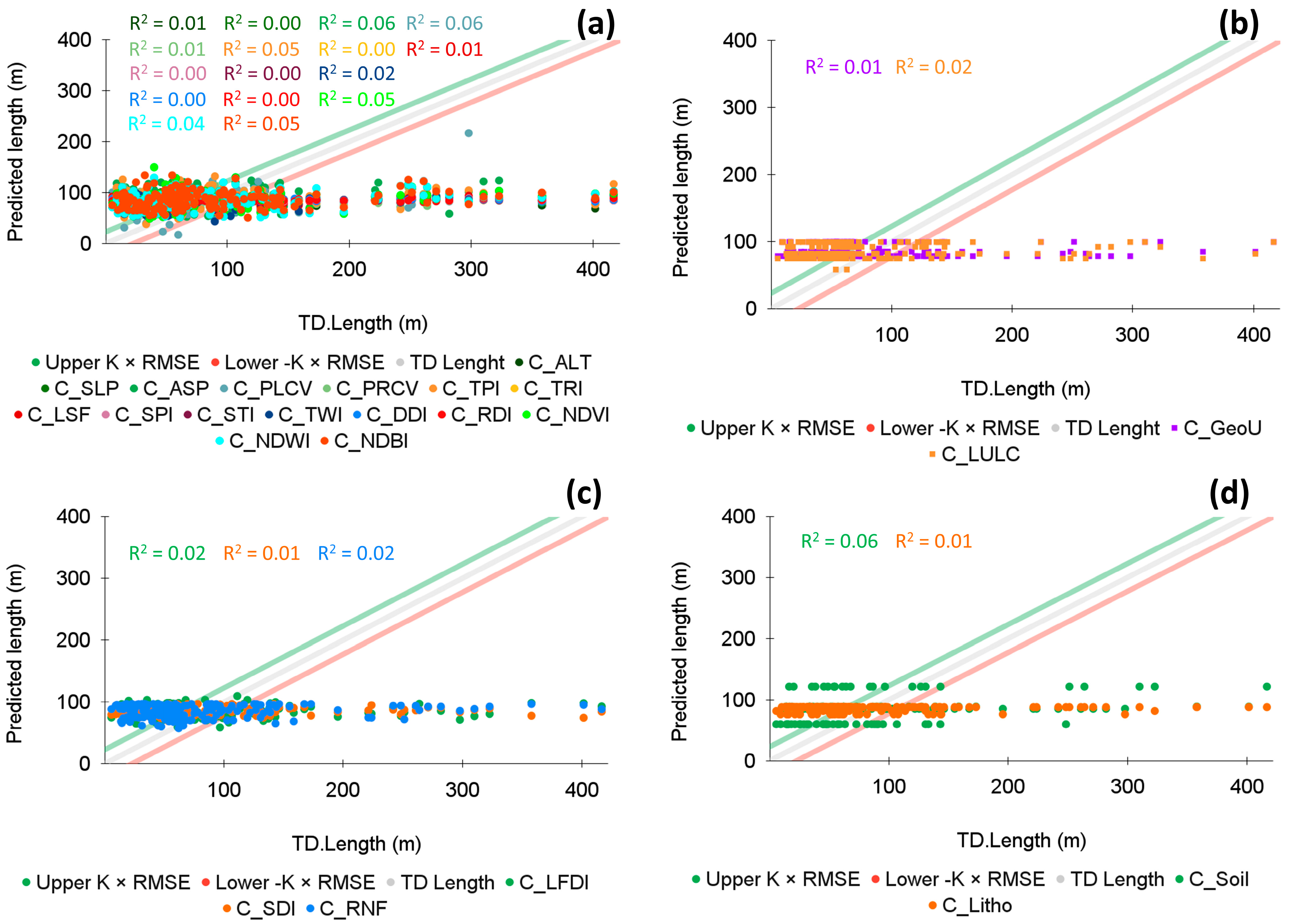
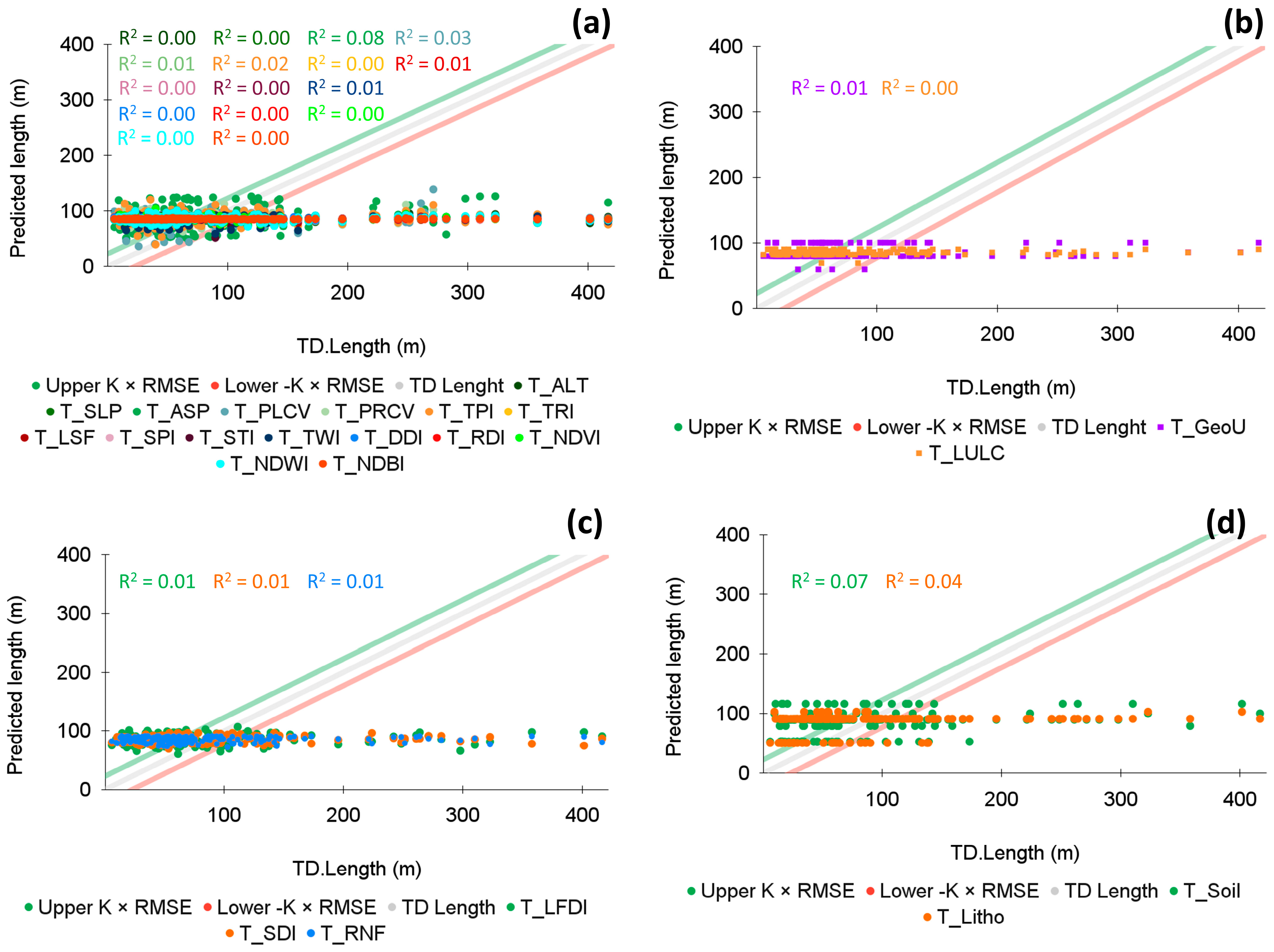
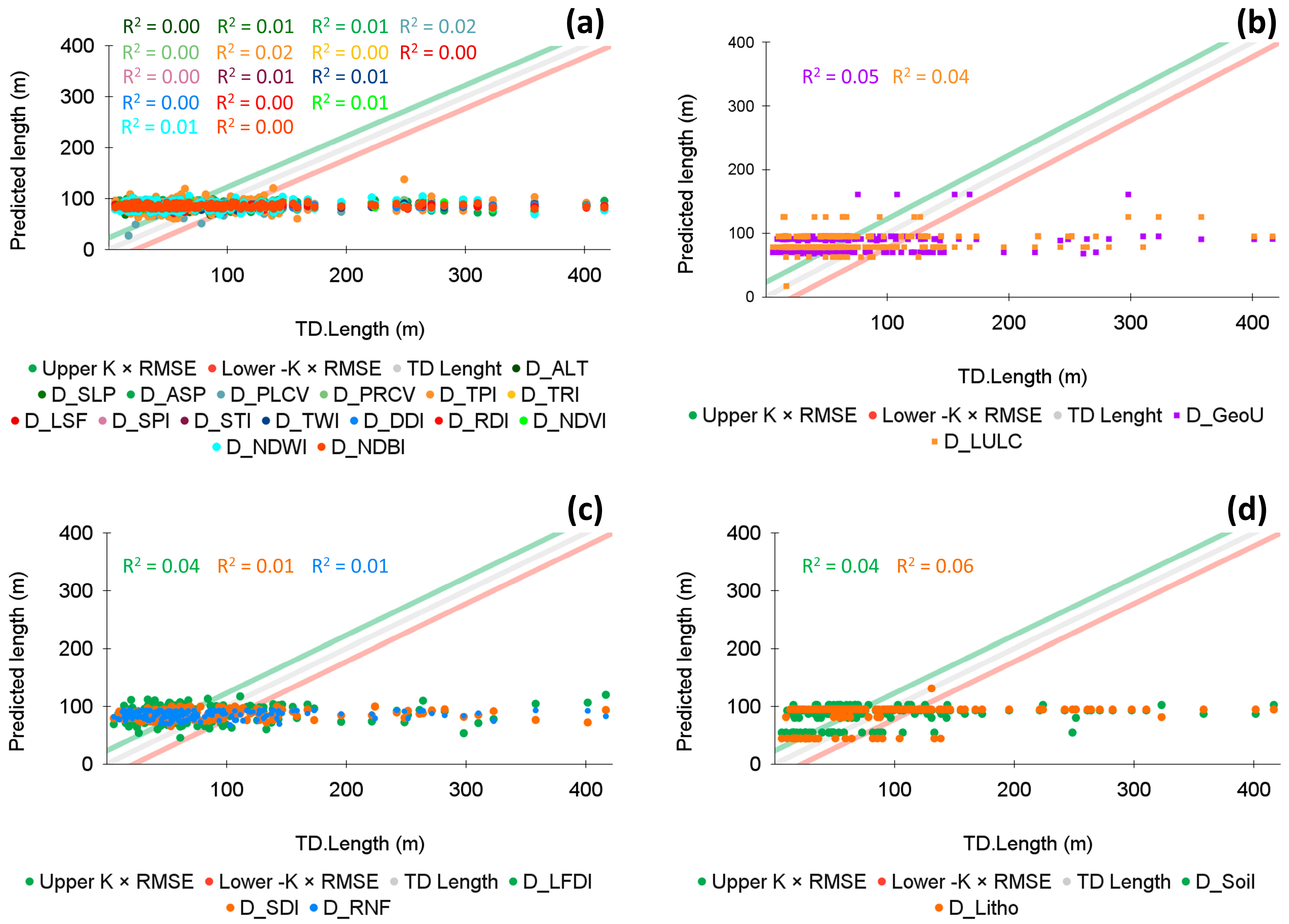
Appendix A.2. Multivariate Linear Regression Models (Types 3 to 6)
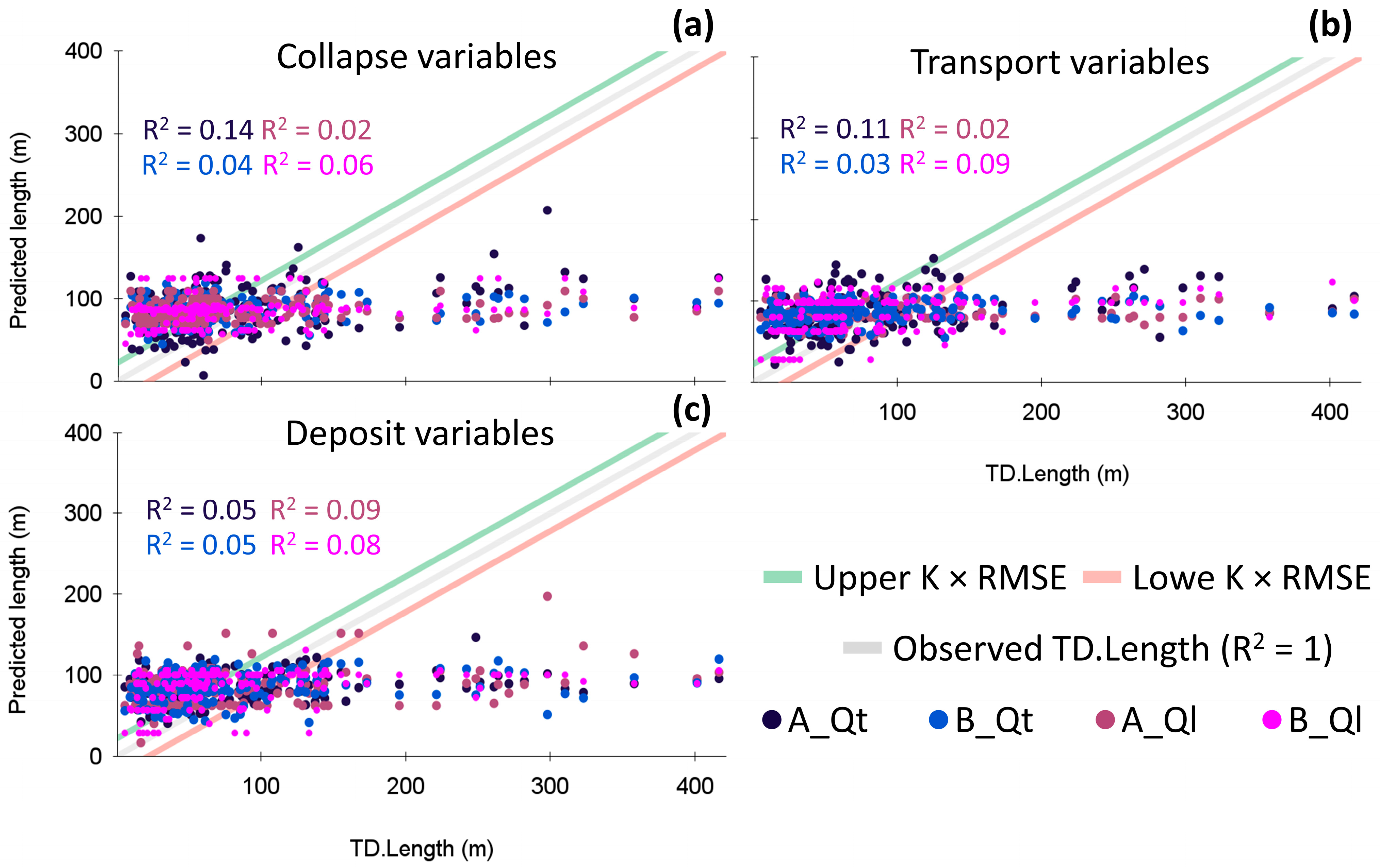
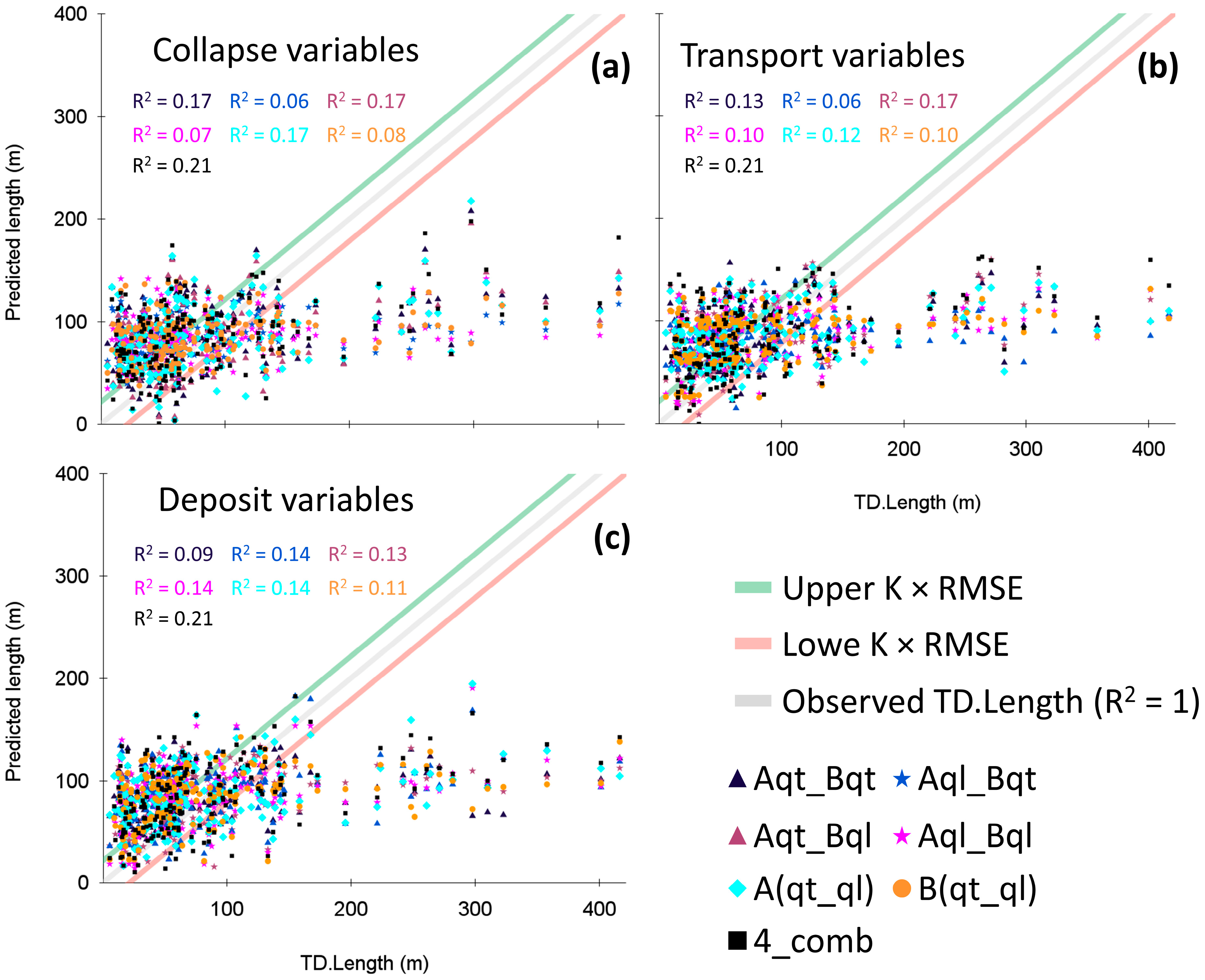
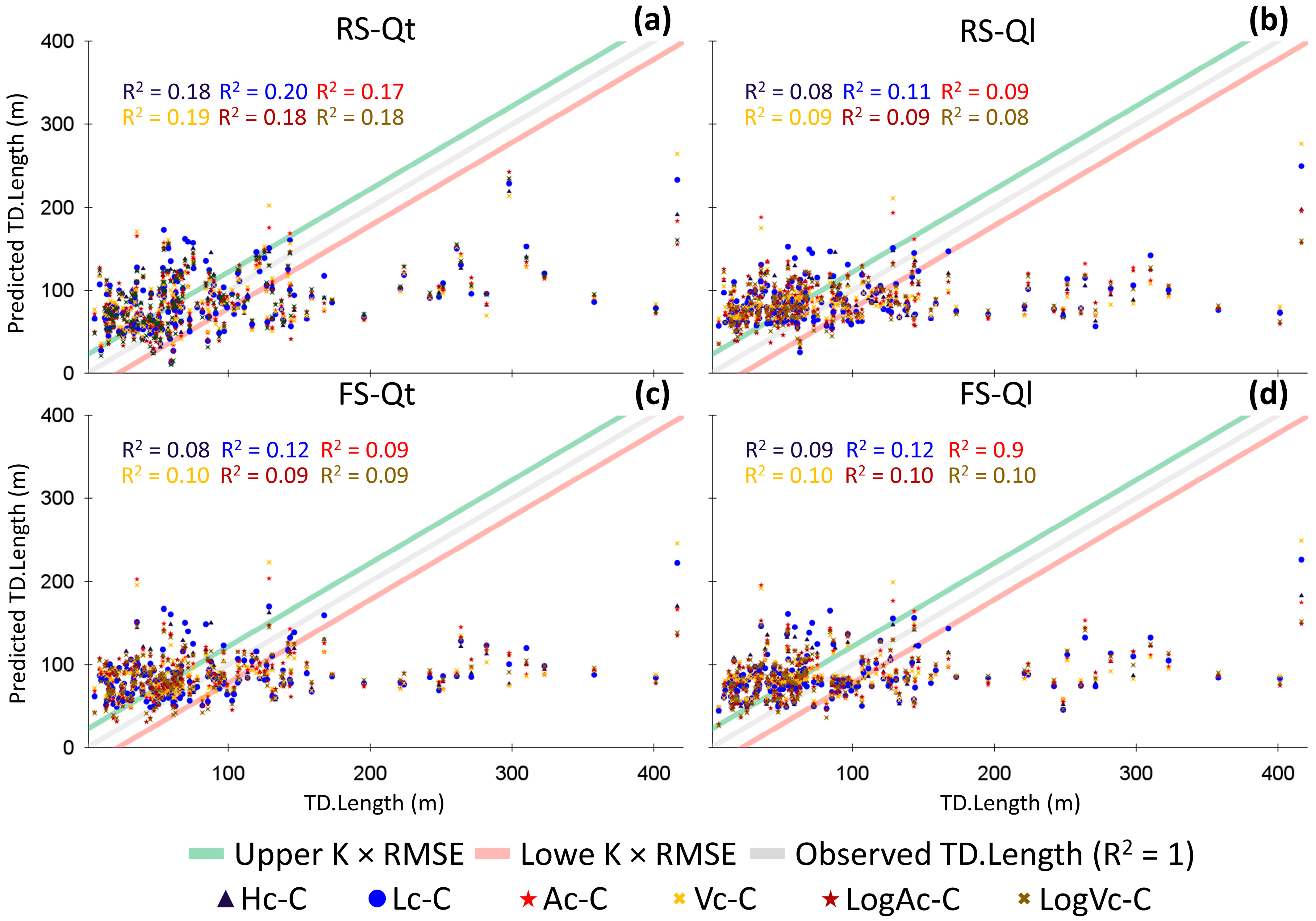
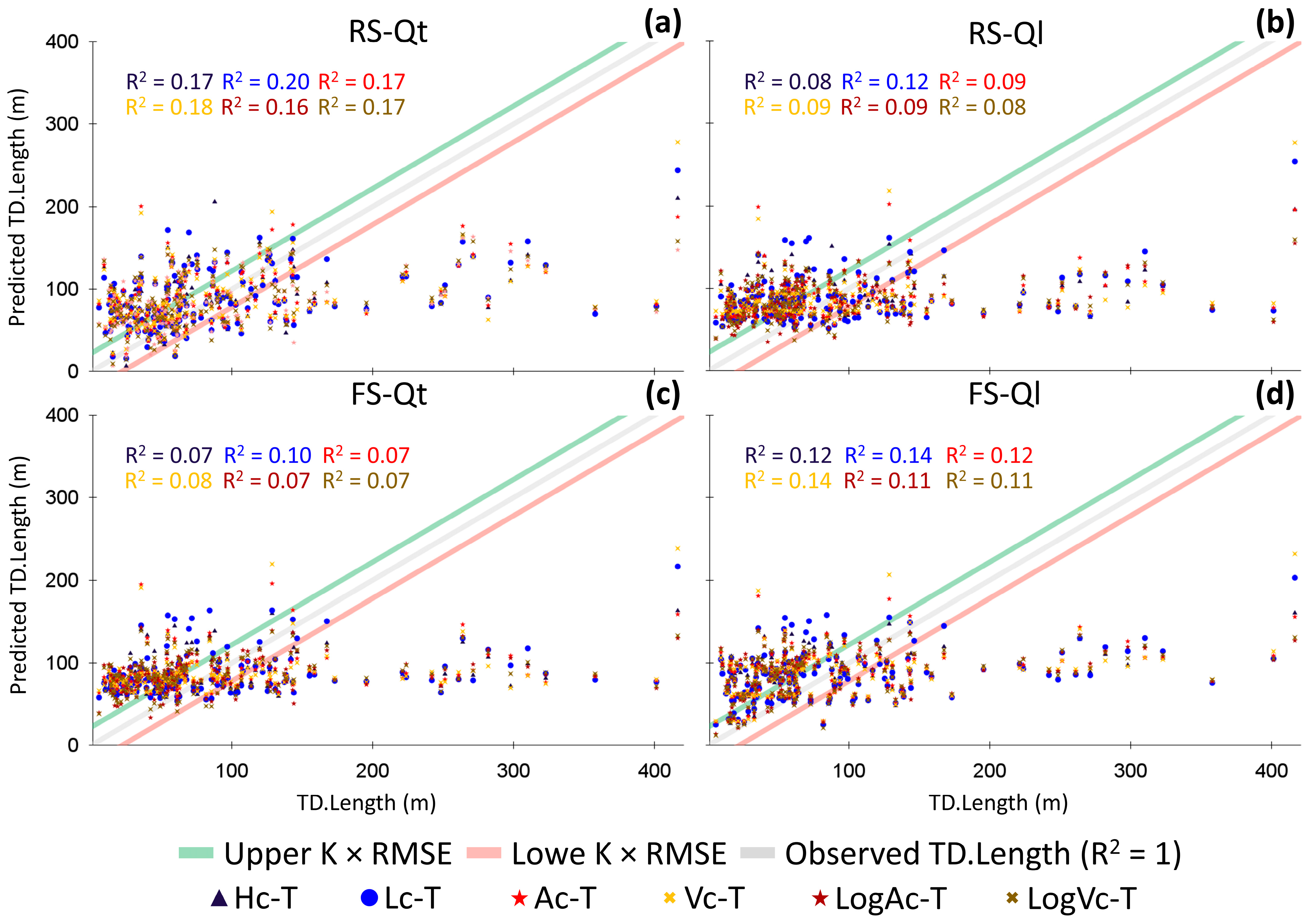
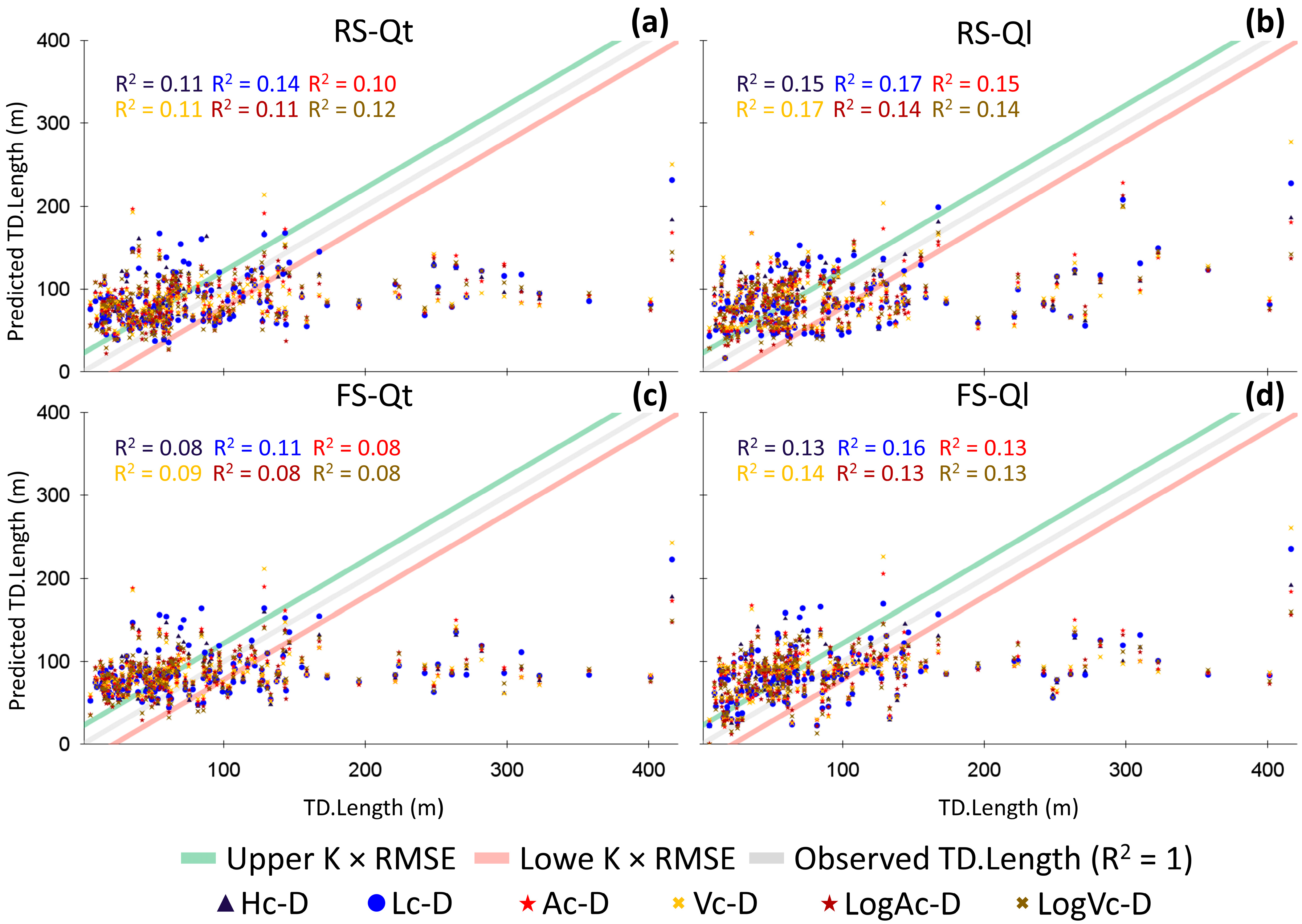
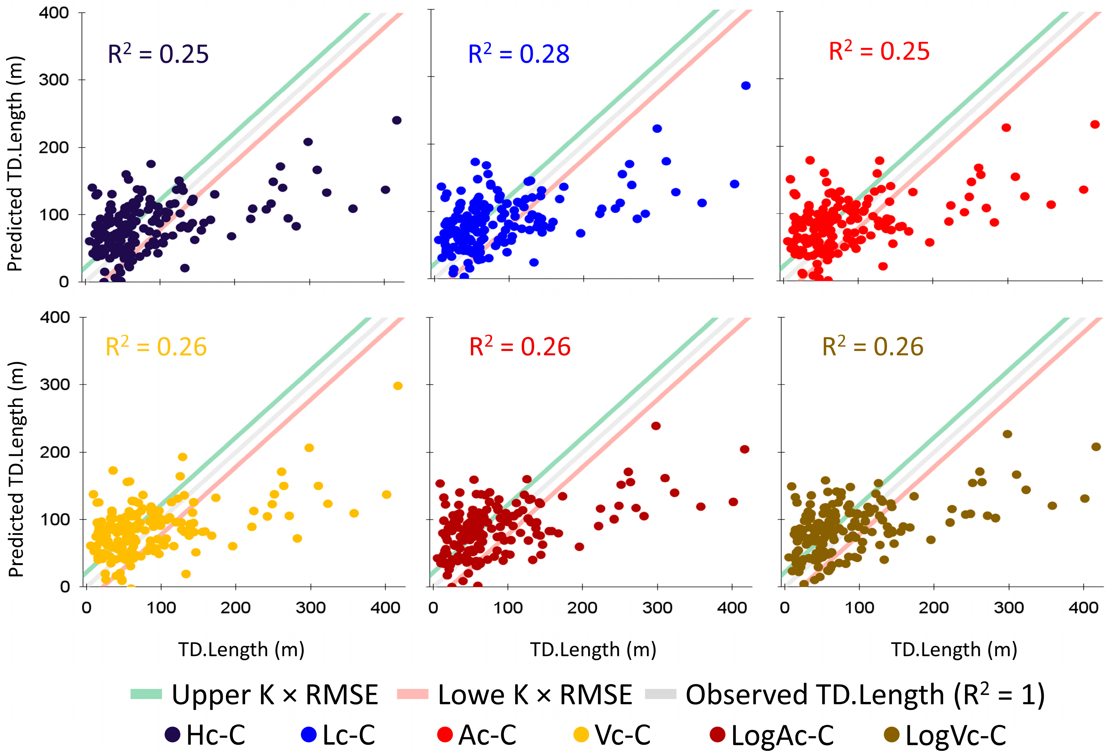
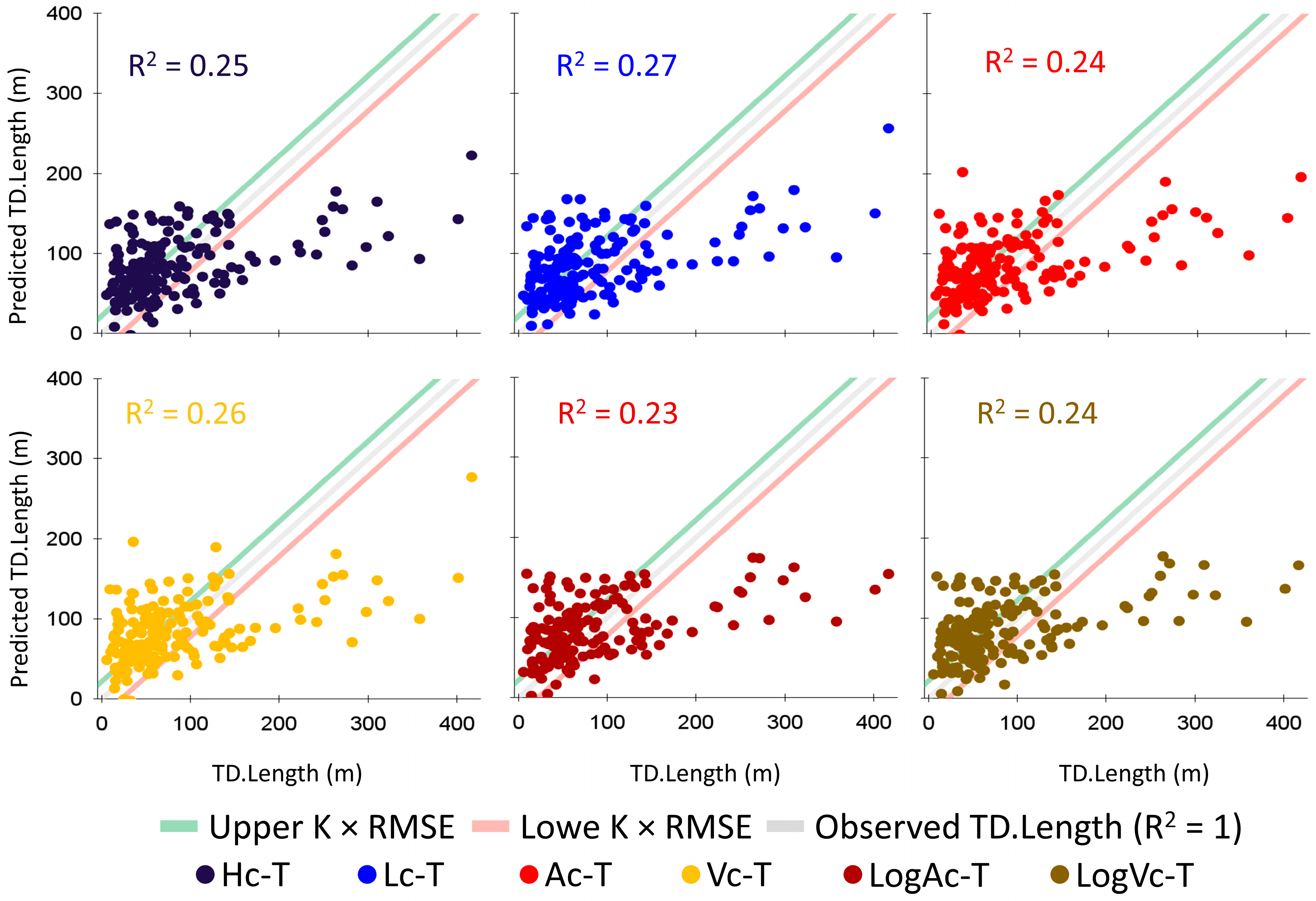

Appendix B. Complete Statistical Analysis for CTD-Based Multivariate Linear Regression Models (Model 8)
Appendix B.1. CTD-Based Model
| Model Fit Measures | Overall Model Test | ||||||
|---|---|---|---|---|---|---|---|
| Model | R2 | Adjusted R2 | RMSE | F | df1 | df2 | p |
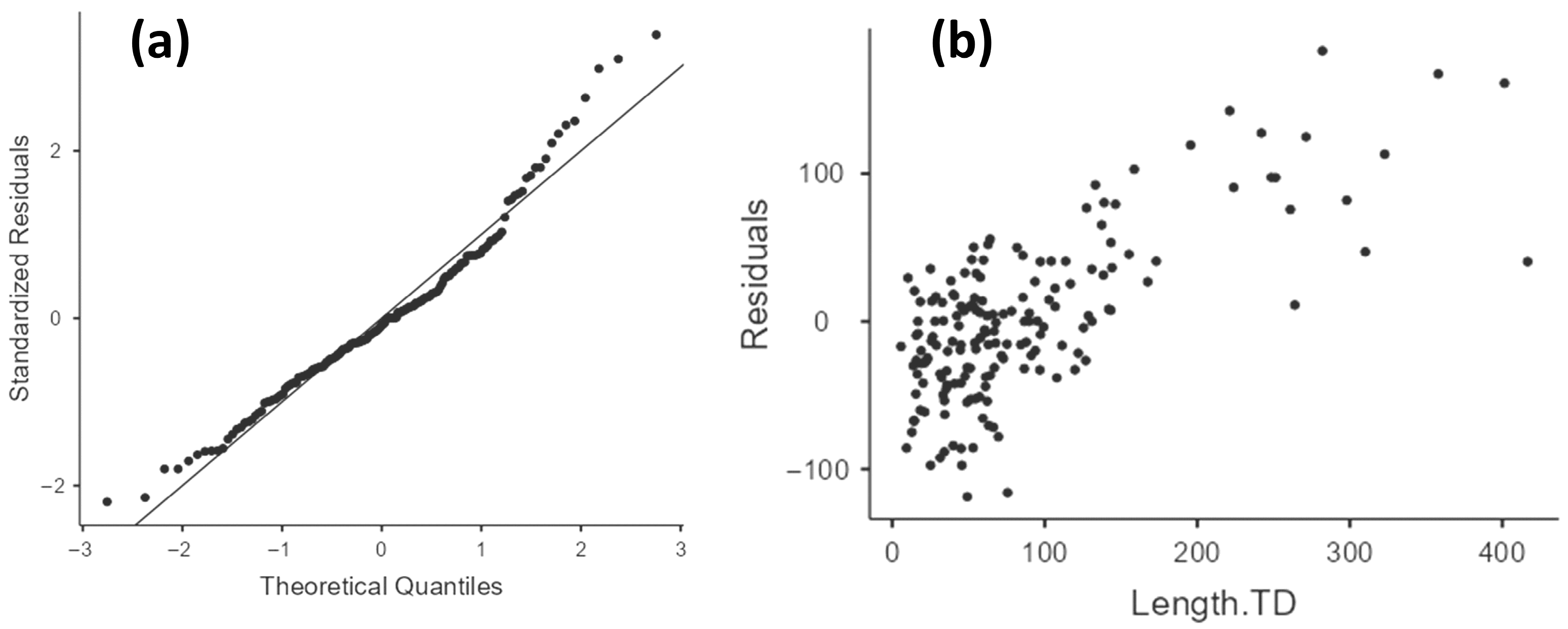
| CTD-based | 0.481 | 0.182 | 55.3 | 1.61 | 62 | 108 | 0.015 |
| Normality Tests | ||
|---|---|---|
| Tests | Statistic | p |
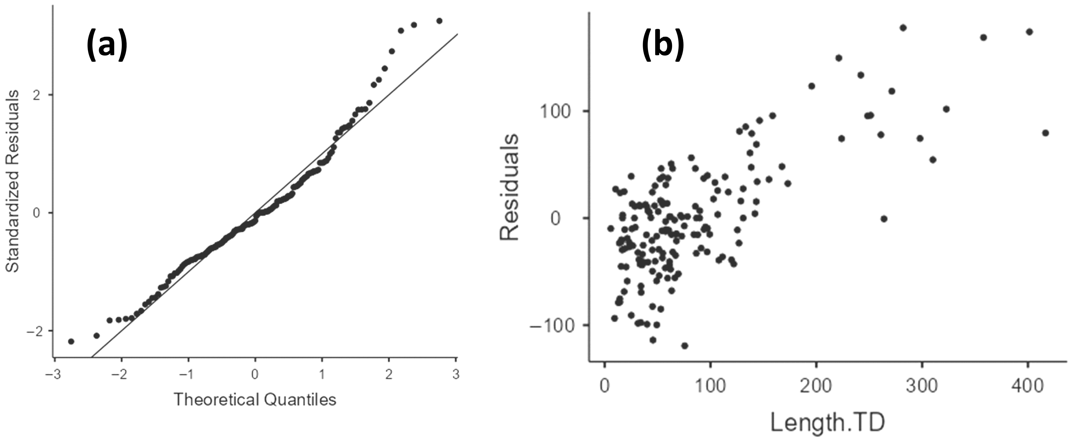
| Shapiro-Wilk | 0.962 | <0.001 |
| Heteroskedasticity Tests | ||
|---|---|---|
| Tests | Statistic | p |
| Breusch-Pagan | 67.8 | 0.288 |
| Durbin–Watson Test for Autocorrelation | ||
|---|---|---|
| Autocorrelation | DW Statistic | p |
| 0.151 | 1.69 | 0.034 |
| Collinearity Statistics | ||
|---|---|---|
| Predictor | VIF | Tolerance |
| D.LULC | 1.33 | 0.752 |
| D.SOIL | 2.79 | 0.358 |
| D.GEOU | 1.77 | 0.564 |
| D.Litho | 1.74 | 0.576 |
| D.ASP | 1.67 | 0.599 |
| D.PLCV | 2.13 | 0.47 |
| D.RNF | 2.77 | 0.361 |
| D.TPI | 1.7 | 0.589 |
| D.TWI | 2.96 | 0.338 |
| D.TRI | 2.27 | 0.441 |
| D.SDI | 2.34 | 0.428 |
| D.NDVI | 1.7 | 0.587 |
| D.LFDI | 3.64 | 0.275 |
| T.PLCV | 2.63 | 0.38 |
| T.TPI | 2.68 | 0.373 |
| T.Litho | 2.05 | 0.488 |
| T.SOIL | 1.61 | 0.623 |
| T.LULC | 1.6 | 0.625 |
| C.ASP | 1.77 | 0.564 |
| C.PLCV | 2.19 | 0.456 |
| C.RNF | 1.27 | 0.784 |
| C.TPI | 2.7 | 0.371 |
| C.TWI | 2.61 | 0.383 |
| C.TRI | 2.53 | 0.396 |
| C.LFDI | 3.46 | 0.289 |
| C.NDVI | 2.34 | 0.427 |
| C.NDBI | 2.22 | 0.451 |
| C.Litho | 1.47 | 0.68 |
| C.GEOU | 2.41 | 0.415 |
| C.SOIL | 3.06 | 0.327 |
| C.LULC | 1.49 | 0.67 |
| Predictor | t | p | Stand. Estimate | 95% Confidence Interval | |
|---|---|---|---|---|---|
| Lower | Upper | ||||
| Intercept a | −0.02662 | 0.979 | |||
| D.LULC: | |||||
| Mosaic of Uses—Forest Formation | 0.79499 | 0.428 | 0.29114 | −0.4348 | 1.017 |
| Pasture—Forest Formation | −0.55371 | 0.581 | −0.23268 | −1.0656 | 0.6003 |
| Rocky Outcrop—Forest Formation | −1.48653 | 0.14 | −1.55343 | −3.6248 | 0.518 |
| Urban Area—Forest Formation | −1.11821 | 0.266 | −0.24297 | −0.6737 | 0.1877 |
| D.SOIL: | |||||
| CXbd4—AR3 | 0.90877 | 0.365 | 1.14162 | −1.3484 | 3.6317 |
| CXbd6—AR3 | 3.10082 | 0.002 | 1.81842 | 0.656 | 2.9808 |
| LVAd24—AR3 | 2.13283 | 0.035 | 1.34112 | 0.0947 | 2.5875 |
| Urban area—AR3 | 3.3246 | 0.001 | 1.74551 | 0.7048 | 2.7862 |
| D.GEOU: | |||||
| Colluvial-talus slopes—Alluvial-colluvial slopes | 0.07752 | 0.938 | 0.04354 | −1.0697 | 1.1568 |
| Dissected hills and low hills—Alluvial-colluvial slopes | −0.38093 | 0.704 | −0.23338 | −1.4478 | 0.981 |
| Floodplains—Alluvial-colluvial slopes | 0.39166 | 0.696 | 0.27552 | −1.1189 | 1.6699 |
| High hills domain—Alluvial-colluvial slopes | −0.48215 | 0.631 | −0.24528 | −1.2537 | 0.7631 |
| Mountainous Domain—Alluvial-colluvial slopes | 0.10314 | 0.918 | 0.06488 | −1.1819 | 1.3116 |
| Mountainous escarpments—Alluvial-colluvial slopes | 0.07194 | 0.943 | 0.05175 | −1.3742 | 1.4777 |
| D.Litho: | |||||
| NP3_gamma_1rnb—NP23_gamma_1rn | −1.53119 | 0.129 | −0.5537 | −1.2705 | 0.1631 |
| NP3_gamma_3so—NP23_gamma_1rn | −1.17646 | 0.242 | −0.72108 | −1.936 | 0.4938 |
| NP3_gamma_3sor—NP23_gamma_1rn | 0.27073 | 0.787 | 0.30479 | −1.9268 | 2.5363 |
| O1_gamma_6nfan—NP23_gamma_1rn | −1.13999 | 0.257 | −1.7855 | −4.8901 | 1.3191 |
| D.ASP | −0.01478 | 0.988 | −0.00171 | −0.2313 | 0.2279 |
| D.PLCV | 0.15219 | 0.879 | 0.02245 | −0.27 | 0.3149 |
| D.RNF | −0.24198 | 0.809 | −0.04643 | −0.4268 | 0.3339 |
| D.TPI | 1.38212 | 0.17 | 0.16273 | −0.0707 | 0.3961 |
| D.TWI | 0.00362 | 0.997 | 7.44 × 10⁻⁴ | −0.4063 | 0.4078 |
| D.TRI | −1.10901 | 0.27 | −0.17436 | −0.486 | 0.1373 |
| D.SDI | 0.54581 | 0.586 | 0.08849 | −0.2329 | 0.4099 |
| D.NDVI | 0.37283 | 0.71 | 0.04401 | −0.19 | 0.278 |
| D.LFDI | −2.07209 | 0.041 | −0.52276 | −1.0228 | −0.0227 |
| T.PLCV | −0.0304 | 0.976 | −0.00555 | −0.3675 | 0.3564 |
| T.TPI | −0.39279 | 0.695 | −0.07294 | −0.441 | 0.2951 |
| T.Litho: | |||||
| NP3_gamma_1rnb—NP23_gamma_1rn | 0.64048 | 0.523 | 0.24076 | −0.5043 | 0.9859 |
| NP3_gamma_3so—NP23_gamma_1rn | 1.09114 | 0.278 | 0.59516 | −0.486 | 1.6763 |
| T.SOIL: | |||||
| CXbd4—AR3 | −0.92449 | 0.357 | −0.42433 | −1.3341 | 0.4855 |
| CXbd6—AR3 | −0.22482 | 0.823 | −0.10161 | −0.9975 | 0.7943 |
| LVAd24—AR3 | −1.72167 | 0.088 | −0.74263 | −1.5976 | 0.1124 |
| Urban area—AR3 | −0.53031 | 0.597 | −0.20147 | −0.9545 | 0.5516 |
| T.LULC: | |||||
| Mosaic of Uses—Forest Formation | −1.18817 | 0.237 | −0.34351 | −0.9166 | 0.2296 |
| Pasture—Forest Formation | 0.25406 | 0.8 | 0.11943 | −0.8124 | 1.0512 |
| Rocky Outcrop—Forest Formation | −1.67884 | 0.096 | −1.59302 | −3.4739 | 0.2878 |
| Urban Area—Forest Formation | 0.37888 | 0.706 | 0.11997 | −0.5077 | 0.7476 |
| C.ASP | 0.38795 | 0.699 | 0.04771 | −0.1961 | 0.2915 |
| C.PLCV | 0.79971 | 0.426 | 0.12162 | −0.1798 | 0.4231 |
| C.RNF | 0.92501 | 0.357 | 0.08178 | −0.0935 | 0.257 |
| C.TPI | 1.7018 | 0.092 | 0.31813 | −0.0524 | 0.6887 |
| C.TWI | 0.19075 | 0.849 | 0.03451 | −0.3241 | 0.3931 |
| C.TRI | −0.52238 | 0.602 | −0.09154 | −0.4389 | 0.2558 |
| C.LFDI | 1.93291 | 0.056 | 0.46319 | −0.0118 | 0.9382 |
| C.NDVI | 0.80754 | 0.421 | 0.13109 | −0.1907 | 0.4529 |
| C.NDBI | 1.6661 | 0.099 | 0.2564 | −0.0486 | 0.5614 |
| C.Litho: | |||||
| NP3_gamma_1rnb—NP23_gamma_1rn | 0.03747 | 0.97 | 0.00933 | −0.4844 | 0.5031 |
| NP3_gamma_3so—NP23_gamma_1rn | −0.26305 | 0.793 | −0.10685 | −0.912 | 0.6983 |
| C.GEOU: | |||||
| Dissected hills and Low hills—Colluvial-Talus slopes | −0.08502 | 0.932 | −0.11678 | −2.8396 | 2.6061 |
| High mountainous domain—Colluvial-Talus slopes | −0.18098 | 0.857 | −0.21352 | −2.552 | 2.125 |
| Mountainous domain—Colluvial-Talus slopes | −0.12987 | 0.897 | −0.17054 | −2.7736 | 2.4325 |
| Mountainous escarpments—Colluvial-Talus slopes | −0.23345 | 0.816 | −0.25682 | −2.4374 | 1.9238 |
| C.SOIL: | |||||
| CXbd4—AR3 | −0.51618 | 0.607 | −0.63197 | −3.0588 | 1.7949 |
| CXbd6—AR3 | −2.48942 | 0.014 | −1.35166 | −2.4279 | −0.2754 |
| LVAd24—AR3 | −1.94157 | 0.055 | −1.25958 | −2.5455 | 0.0263 |
| Urban area—AR3 | −2.80229 | 0.006 | −1.53099 | −2.6139 | −0.4481 |
| C.LULC: | |||||
| Mosaic of Uses—Forest Formation | −1.14997 | 0.253 | −0.30729 | −0.8369 | 0.2224 |
| Pasture—Forest Formation | −1.62091 | 0.108 | −0.64037 | −1.4235 | 0.1427 |
| Rocky Outcrop—Forest Formation | −1.33743 | 0.184 | −1.23602 | −3.0679 | 0.5959 |
| Urban Area—Forest Formation | −1.00868 | 0.315 | −0.31439 | −0.9322 | 0.3034 |
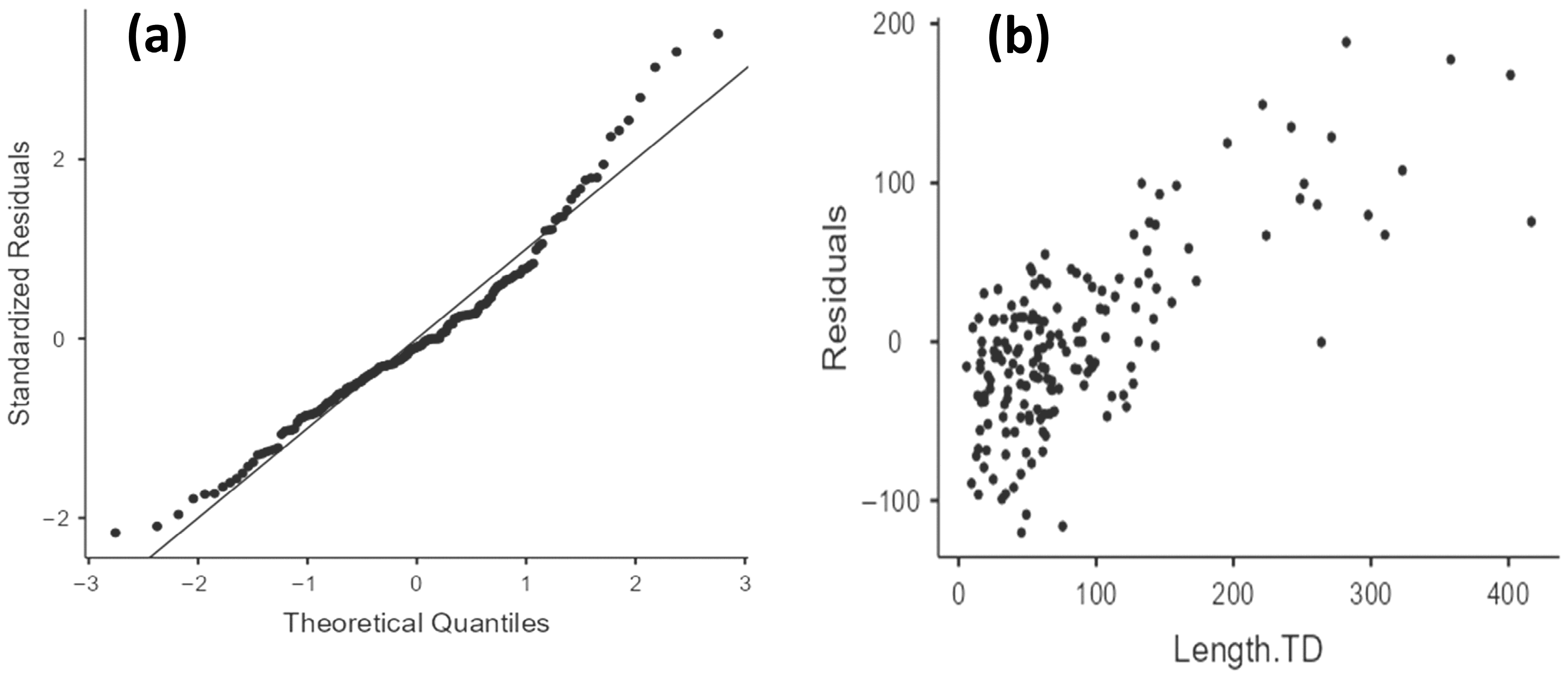
Appendix B.2. Hc-CTD Model
| Model Fit Measures | Overall Model Test | ||||||
|---|---|---|---|---|---|---|---|
| Model | R2 | Adjusted R2 | RMSE | F | df1 | df2 | p |
| Hc_CTD | 0.491 | 0.191 | 54.7 | 1.64 | 63 | 107 | 0.012 |
| Normality Tests | ||
|---|---|---|
| Tests | Statistic | p |
| Shapiro–Wilk | 0.96 | <0.001 |
| Heteroskedasticity Tests | ||
|---|---|---|
| Tests | Statistic | p |
| Breusch-Pagan | 68.5 | 0.296 |
| Durbin–Watson Test for Autocorrelation | ||
|---|---|---|
| Autocorrelation | DW Statistic | p |
| 0.151 | 1.69 | 0.034 |
| Collinearity Statistics | ||
|---|---|---|
| Predictor | VIF | Tolerance |
| D.LULC | 1.34 | 0.747 |
| D.SOIL | 2.82 | 0.355 |
| D.GEOU | 1.78 | 0.561 |
| D.Litho | 1.74 | 0.575 |
| D.ASP | 1.68 | 0.594 |
| D.PLCV | 2.14 | 0.466 |
| D.RNF | 2.77 | 0.361 |
| D.TPI | 1.7 | 0.589 |
| D.TWI | 3.01 | 0.332 |
| D.TRI | 2.27 | 0.441 |
| D.SDI | 2.34 | 0.428 |
| D.NDVI | 1.72 | 0.583 |
| D.LFDI | 3.75 | 0.267 |
| T.PLCV | 2.65 | 0.378 |
| T.TPI | 2.77 | 0.361 |
| T.Litho | 2.05 | 0.488 |
| T.SOIL | 1.61 | 0.621 |
| T.LULC | 1.6 | 0.623 |
| C.ASP | 1.79 | 0.558 |
| C.PLCV | 2.19 | 0.456 |
| C.RNF | 1.28 | 0.78 |
| C.TPI | 2.93 | 0.342 |
| C.TWI | 2.61 | 0.383 |
| C.TRI | 2.55 | 0.392 |
| C.LFDI | 3.52 | 0.284 |
| C.NDVI | 2.36 | 0.423 |
| C.NDBI | 2.22 | 0.451 |
| C.Litho | 1.48 | 0.678 |
| C.GEOU | 2.42 | 0.413 |
| C.SOIL | 3.11 | 0.322 |
| C.LULC | 1.5 | 0.666 |
| Height.C | 1.85 | 0.542 |
| Predictor | t | p | Stand. Estimate | 95% Confidence Interval | |
|---|---|---|---|---|---|
| Lower | Upper | ||||
| Intercept a | −0.01131 | 0.991 | |||
| D.LULC: | |||||
| Mosaic of Uses—Forest Formation | 1.03494 | 0.303 | 0.38234 | −0.35 | 1.1147 |
| Pasture—Forest Formation | −0.67628 | 0.5 | −0.2836 | −1.1149 | 0.5477 |
| Rocky Outcrop—Forest Formation | −1.48719 | 0.14 | −1.54573 | −3.6061 | 0.5147 |
| Urban Area—Forest Formation | −0.92089 | 0.359 | −0.20075 | −0.6329 | 0.2314 |
| D.SOIL: | |||||
| CXbd4—AR3 | 0.76566 | 0.446 | 0.9612 | −1.5275 | 3.4499 |
| CXbd6—AR3 | 2.80475 | 0.006 | 1.66249 | 0.4874 | 2.8375 |
| LVAd24—AR3 | 1.84766 | 0.067 | 1.17423 | −0.0856 | 2.4341 |
| Urban area—AR3 | 2.89316 | 0.005 | 1.55582 | 0.4898 | 2.6219 |
| D.GEOU: | |||||
| Colluvial-talus slopes—Alluvial-colluvial slopes | 0.03138 | 0.975 | 0.01754 | −1.0903 | 1.1254 |
| Dissected hills and low hills—Alluvial-colluvial slopes | −0.52782 | 0.599 | −0.32322 | −1.5372 | 0.8907 |
| Floodplains—Alluvial-colluvial slopes | 0.43463 | 0.665 | 0.3042 | −1.0833 | 1.6917 |
| High hills domain—Alluvial-colluvial slopes | −0.60981 | 0.543 | −0.30969 | −1.3165 | 0.6971 |
| Mountainous Domain—Alluvial-colluvial slopes | 0.00388 | 0.997 | 0.00243 | −1.2405 | 1.2454 |
| Mountainous escarpments—Alluvial-colluvial slopes | 0.1442 | 0.886 | 0.1033 | −1.3168 | 1.5234 |
| D.Litho: | |||||
| NP3_gamma_1rnb—NP23_gamma_1rn | −1.42221 | 0.158 | −0.51301 | −1.2281 | 0.2021 |
| NP3_gamma_3so—NP23_gamma_1rn | −1.23207 | 0.221 | −0.7515 | −1.9607 | 0.4577 |
| NP3_gamma_3sor—NP23_gamma_1rn | 0.21918 | 0.827 | 0.24557 | −1.9755 | 2.4667 |
| O1_gamma_6nfan—NP23_gamma_1rn | −1.09037 | 0.278 | −1.69972 | −4.79 | 1.3905 |
| D.ASP | −0.19237 | 0.848 | −0.02232 | −0.2524 | 0.2077 |
| D.PLCV | −0.02918 | 0.977 | −0.00431 | −0.2974 | 0.2888 |
| D.RNF | −0.1986 | 0.843 | −0.03792 | −0.4164 | 0.3406 |
| D.TPI | 1.3636 | 0.176 | 0.15971 | −0.0725 | 0.3919 |
| D.TWI | −0.25878 | 0.796 | −0.0537 | −0.4651 | 0.3577 |
| D.TRI | −1.09744 | 0.275 | −0.17162 | −0.4816 | 0.1384 |
| D.SDI | 0.59064 | 0.556 | 0.09528 | −0.2245 | 0.4151 |
| D.NDVI | 0.55239 | 0.582 | 0.06534 | −0.1692 | 0.2998 |
| D.LFDI | −1.66243 | 0.099 | −0.43001 | −0.9428 | 0.0828 |
| T.PLCV | 0.11063 | 0.912 | 0.02019 | −0.3415 | 0.3819 |
| T.TPI | 2.31 × 10⁻⁴ | 1 | 4.42 × 10⁻⁵ | −0.379 | 0.3791 |
| T.Litho: | |||||
| NP3_gamma_1rnb—NP23_gamma_1rn | 0.67696 | 0.5 | 0.25316 | −0.4882 | 0.9945 |
| NP3_gamma_3so—NP23_gamma_1rn | 0.9881 | 0.325 | 0.53743 | −0.5408 | 1.6156 |
| T.SOIL: | |||||
| CXbd4—AR3 | −1.13608 | 0.258 | −0.5243 | −1.4392 | 0.3906 |
| CXbd6—AR3 | −0.32566 | 0.745 | −0.14673 | −1.0399 | 0.7465 |
| LVAd24—AR3 | −1.8563 | 0.066 | −0.79958 | −1.6535 | 0.0543 |
| Urban area—AR3 | −0.66917 | 0.505 | −0.25396 | −1.0063 | 0.4984 |
| T.LULC: | |||||
| Mosaic of Uses—Forest Formation | −1.06871 | 0.288 | −0.30835 | −0.8803 | 0.2636 |
| Pasture—Forest Formation | 0.48666 | 0.627 | 0.23046 | −0.7083 | 1.1692 |
| Rocky Outcrop—Forest Formation | −1.55474 | 0.123 | −1.47274 | −3.3506 | 0.4051 |
| Urban Area—Forest Formation | 0.42252 | 0.673 | 0.13311 | −0.4914 | 0.7577 |
| C.ASP | 0.59427 | 0.554 | 0.07342 | −0.1715 | 0.3183 |
| C.PLCV | 0.76708 | 0.445 | 0.11606 | −0.1839 | 0.416 |
| C.RNF | 0.76389 | 0.447 | 0.06757 | −0.1078 | 0.2429 |
| C.TPI | 0.99905 | 0.32 | 0.20175 | −0.1986 | 0.6021 |
| C.TWI | 0.25752 | 0.797 | 0.04638 | −0.3107 | 0.4034 |
| C.TRI | −0.71045 | 0.479 | −0.12485 | −0.4732 | 0.2235 |
| C.LFDI | 1.63574 | 0.105 | 0.39675 | −0.0841 | 0.8776 |
| C.NDVI | 1.00636 | 0.317 | 0.16403 | −0.1591 | 0.4871 |
| C.NDBI | 1.69222 | 0.094 | 0.25902 | −0.0444 | 0.5625 |
| C.Litho: | |||||
| NP3_gamma_1rnb—NP23_gamma_1rn | −0.03584 | 0.971 | −0.00889 | −0.5006 | 0.4828 |
| NP3_gamma_3so—NP23_gamma_1rn | −0.11083 | 0.912 | −0.04502 | −0.8502 | 0.7602 |
| C.GEOU: | |||||
| Dissected hills and Low hills—Colluvial-Talus slopes | −0.06633 | 0.947 | −0.09063 | −2.7992 | 2.618 |
| High mountainous domain—Colluvial-Talus slopes | −0.20676 | 0.837 | −0.24264 | −2.5691 | 2.0838 |
| Mountainous domain—Colluvial-Talus slopes | −0.02832 | 0.977 | −0.03708 | −2.6325 | 2.5583 |
| Mountainous escarpments—Colluvial-Talus slopes | −0.28465 | 0.776 | −0.31163 | −2.4819 | 1.8586 |
| C.SOIL: | |||||
| CXbd4—AR3 | −0.26438 | 0.792 | −0.32655 | −2.7751 | 2.122 |
| CXbd6—AR3 | −2.22129 | 0.028 | −1.21662 | −2.3024 | −0.1309 |
| LVAd24—AR3 | −1.54613 | 0.125 | −1.02692 | −2.3436 | 0.2898 |
| Urban area—AR3 | −2.16284 | 0.033 | −1.24679 | −2.3896 | −0.104 |
| C.LULC: | |||||
| Mosaic of Uses—Forest Formation | −1.31664 | 0.191 | −0.3522 | −0.8825 | 0.1781 |
| Pasture—Forest Formation | −1.81412 | 0.072 | −0.7194 | −1.5055 | 0.0667 |
| Rocky Outcrop—Forest Formation | −1.50525 | 0.135 | −1.39278 | −3.227 | 0.4415 |
| Urban Area—Forest Formation | −0.93517 | 0.352 | −0.2903 | −0.9057 | 0.3251 |
| Height.C | 1.4764 | 0.143 | 0.18792 | −0.0644 | 0.4402 |
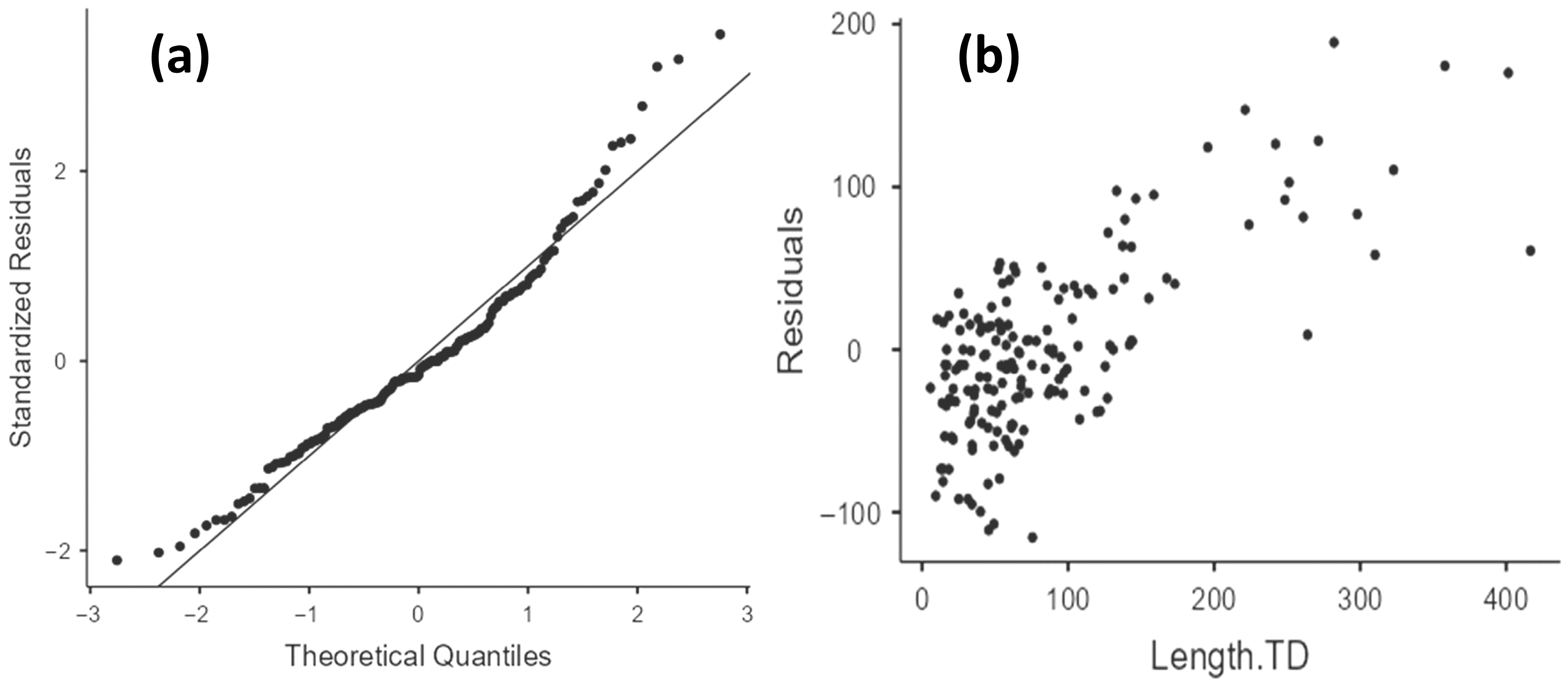
Appendix B.3. Lc-CTD Model
| Model Fit Measures | Overall Model Test | ||||||
|---|---|---|---|---|---|---|---|
| Model | R2 | Adjusted R2 | RMSE | F | df1 | df2 | p |
| Lc_CTD | 0.507 | 0.217 | 53.9 | 1.75 | 63 | 107 | 0.006 |
| Normality Tests | ||
|---|---|---|
| Tests | Statistic | p |
| Shapiro-Wilk | 0.965 | <0.001 |
| Heteroskedasticity Tests | ||
|---|---|---|
| Tests | Statistic | p |
| Breusch-Pagan | 70.2 | 0.248 |
| Durbin–Watson Test for Autocorrelation | ||
|---|---|---|
| Autocorrelation | DW Statistic | p |
| 0.161 | 1.68 | 0.022 |
| Collinearity Statistics | ||
|---|---|---|
| Predictor | VIF | Tolerance |
| D.LULC | 1.34 | 0.747 |
| D.SOIL | 2.81 | 0.356 |
| D.GEOU | 1.78 | 0.561 |
| D.Litho | 1.74 | 0.575 |
| D.ASP | 1.68 | 0.596 |
| D.PLCV | 2.14 | 0.467 |
| D.RNF | 2.78 | 0.359 |
| D.TPI | 1.7 | 0.589 |
| D.TWI | 2.98 | 0.335 |
| D.TRI | 2.28 | 0.439 |
| D.SDI | 2.35 | 0.425 |
| D.NDVI | 1.71 | 0.584 |
| D.LFDI | 3.71 | 0.269 |
| T.PLCV | 2.67 | 0.374 |
| T.TPI | 2.71 | 0.369 |
| T.Litho | 2.05 | 0.488 |
| T.SOIL | 1.61 | 0.621 |
| T.LULC | 1.61 | 0.622 |
| C.ASP | 1.78 | 0.563 |
| C.PLCV | 2.2 | 0.455 |
| C.RNF | 1.28 | 0.784 |
| C.TPI | 2.81 | 0.356 |
| C.TWI | 2.61 | 0.383 |
| C.TRI | 2.53 | 0.395 |
| C.LFDI | 3.52 | 0.284 |
| C.NDVI | 2.36 | 0.424 |
| C.NDBI | 2.22 | 0.45 |
| C.Litho | 1.47 | 0.679 |
| C.GEOU | 2.41 | 0.414 |
| C.SOIL | 3.12 | 0.321 |
| C.LULC | 1.51 | 0.661 |
| Length.C | 1.84 | 0.544 |
| Predictor | t | p | Stand. Estimate | 95% Confidence Interval | |
|---|---|---|---|---|---|
| Lower | Upper | ||||
| Intercept a | 0.2068 | 0.837 | |||
| D.LULC: | |||||
| Mosaic of Uses—Forest Formation | 1.1846 | 0.239 | 0.43012 | −0.2897 | 1.1499 |
| Pasture—Forest Formation | −0.6608 | 0.51 | −0.27201 | −1.088 | 0.544 |
| Rocky Outcrop—Forest Formation | −1.4939 | 0.138 | −1.52807 | −3.5558 | 0.4996 |
| Urban Area—Forest Formation | −0.7461 | 0.457 | −0.16072 | −0.5878 | 0.2663 |
| D.SOIL: | |||||
| CXbd4—AR3 | 0.9116 | 0.364 | 1.12092 | −1.3165 | 3.5584 |
| CXbd6—AR3 | 2.6793 | 0.009 | 1.56392 | 0.4068 | 2.7211 |
| LVAd24—AR3 | 2.0049 | 0.047 | 1.23696 | 0.0139 | 2.46 |
| Urban area—AR3 | 2.9471 | 0.004 | 1.53618 | 0.5029 | 2.5695 |
| D.GEOU: | |||||
| Colluvial-talus slopes—Alluvial-colluvial slopes | −0.1004 | 0.92 | −0.05535 | −1.1481 | 1.0374 |
| Dissected hills and low hills—Alluvial-colluvial slopes | −0.642 | 0.522 | −0.38718 | −1.5827 | 0.8083 |
| Floodplains—Alluvial-colluvial slopes | 0.152 | 0.879 | 0.10519 | −1.2669 | 1.4773 |
| High hills domain—Alluvial-colluvial slopes | −0.8407 | 0.402 | −0.42323 | −1.4212 | 0.5748 |
| Mountainous Domain—Alluvial-colluvial slopes | 0.1772 | 0.86 | 0.10915 | −1.1118 | 1.3301 |
| Mountainous escarpments—Alluvial-colluvial slopes | 0.103 | 0.918 | 0.07253 | −1.3234 | 1.4685 |
| D.Litho: | |||||
| NP3_gamma_1rnb—NP23_gamma_1rn | −1.5703 | 0.119 | −0.55578 | −1.2574 | 0.1458 |
| NP3_gamma_3so—NP23_gamma_1rn | −1.0864 | 0.28 | −0.65245 | −1.843 | 0.5381 |
| NP3_gamma_3sor—NP23_gamma_1rn | 0.3443 | 0.731 | 0.3795 | −1.8057 | 2.5647 |
| O1_gamma_6nfan—NP23_gamma_1rn | −1.1865 | 0.238 | −1.819 | −4.858 | 1.22 |
| D.ASP | −0.227 | 0.821 | −0.02584 | −0.2515 | 0.1998 |
| D.PLCV | −0.1286 | 0.898 | −0.0187 | −0.307 | 0.2696 |
| D.RNF | −0.4949 | 0.622 | −0.09345 | −0.4678 | 0.2809 |
| D.TPI | 1.4421 | 0.152 | 0.1662 | −0.0623 | 0.3947 |
| D.TWI | −0.2967 | 0.767 | −0.0601 | −0.4617 | 0.3415 |
| D.TRI | −0.9162 | 0.362 | −0.14154 | −0.4478 | 0.1647 |
| D.SDI | 0.8045 | 0.423 | 0.12837 | −0.1879 | 0.4447 |
| D.NDVI | 0.6561 | 0.513 | 0.07632 | −0.1543 | 0.3069 |
| D.LFDI | −1.5912 | 0.115 | −0.40113 | −0.9009 | 0.0986 |
| T.PLCV | 0.3901 | 0.697 | 0.07083 | −0.2891 | 0.4307 |
| T.TPI | −0.0464 | 0.963 | −0.00852 | −0.3727 | 0.3557 |
| T.Litho: | |||||
| NP3_gamma_1rnb—NP23_gamma_1rn | 0.7983 | 0.426 | 0.29423 | −0.4365 | 1.0249 |
| NP3_gamma_3so—NP23_gamma_1rn | 1.174 | 0.243 | 0.62691 | −0.4317 | 1.6855 |
| T.SOIL: | |||||
| CXbd4—AR3 | −1.1393 | 0.257 | −0.51356 | −1.4072 | 0.3801 |
| CXbd6—AR3 | −0.5519 | 0.582 | −0.2464 | −1.1315 | 0.6387 |
| LVAd24—AR3 | −1.946 | 0.054 | −0.82422 | −1.6639 | 0.0154 |
| Urban area—AR3 | −0.7148 | 0.476 | −0.26649 | −1.0056 | 0.4726 |
| T.LULC: | |||||
| Mosaic of Uses—Forest Formation | −1.0584 | 0.292 | −0.30011 | −0.8622 | 0.262 |
| Pasture—Forest Formation | 0.7333 | 0.465 | 0.34432 | −0.5866 | 1.2752 |
| Rocky Outcrop—Forest Formation | −1.7444 | 0.084 | −1.62021 | −3.4614 | 0.221 |
| Urban Area—Forest Formation | 0.4215 | 0.674 | 0.13063 | −0.4838 | 0.745 |
| C.ASP | 0.5134 | 0.609 | 0.06187 | −0.177 | 0.3008 |
| C.PLCV | 0.6288 | 0.531 | 0.09388 | −0.2021 | 0.3898 |
| C.RNF | 0.8486 | 0.398 | 0.07349 | −0.0982 | 0.2452 |
| C.TPI | 1.0043 | 0.318 | 0.19128 | −0.1863 | 0.5689 |
| C.TWI | 0.3033 | 0.762 | 0.05375 | −0.2976 | 0.4051 |
| C.TRI | −0.673 | 0.502 | −0.11563 | −0.4562 | 0.225 |
| C.LFDI | 1.4958 | 0.138 | 0.35703 | −0.1161 | 0.8302 |
| C.NDVI | 1.1128 | 0.268 | 0.17815 | −0.1392 | 0.4955 |
| C.NDBI | 1.8337 | 0.069 | 0.27663 | −0.0224 | 0.5757 |
| C.Litho: | |||||
| NP3_gamma_1rnb—NP23_gamma_1rn | 0.2216 | 0.825 | 0.05419 | −0.4305 | 0.5389 |
| NP3_gamma_3so—NP23_gamma_1rn | −0.2154 | 0.83 | −0.08567 | −0.874 | 0.7027 |
| C.GEOU: | |||||
| Dissected hills and Low hills—Colluvial-Talus slopes | −0.0708 | 0.944 | −0.09517 | −2.7605 | 2.5702 |
| High mountainous domain—Colluvial-Talus slopes | −0.2205 | 0.826 | −0.25468 | −2.544 | 2.0346 |
| Mountainous domain—Colluvial-Talus slopes | −0.1178 | 0.906 | −0.15141 | −2.6995 | 2.3966 |
| Mountainous escarpments—Colluvial-Talus slopes | −0.3395 | 0.735 | −0.36588 | −2.5023 | 1.7705 |
| C.SOIL: | |||||
| CXbd4—AR3 | −0.2755 | 0.783 | −0.33192 | −2.7204 | 2.0565 |
| CXbd6—AR3 | −1.8605 | 0.066 | −1.02142 | −2.1098 | 0.0669 |
| LVAd24—AR3 | −1.4818 | 0.141 | −0.95904 | −2.2421 | 0.324 |
| Urban area—AR3 | −1.8776 | 0.063 | −1.06762 | −2.1948 | 0.0596 |
| C.LULC: | |||||
| Mosaic of Uses—Forest Formation | −1.6953 | 0.093 | −0.45563 | −0.9884 | 0.0772 |
| Pasture—Forest Formation | −2.2072 | 0.029 | −0.88199 | −1.6741 | −0.0898 |
| Rocky Outcrop—Forest Formation | −1.6959 | 0.093 | −1.55005 | −3.3619 | 0.2618 |
| Urban Area—Forest Formation | −1.0293 | 0.306 | −0.31399 | −0.9187 | 0.2907 |
| Length.C | 2.3962 | 0.018 | 0.29893 | 0.0516 | 0.5462 |
Appendix B.4. Ac-CTD Model
| Model Fit Measures | Overall Model Test | ||||||
|---|---|---|---|---|---|---|---|
| Model | R2 | Adjusted R2 | RMSE | F | df1 | df2 | p |
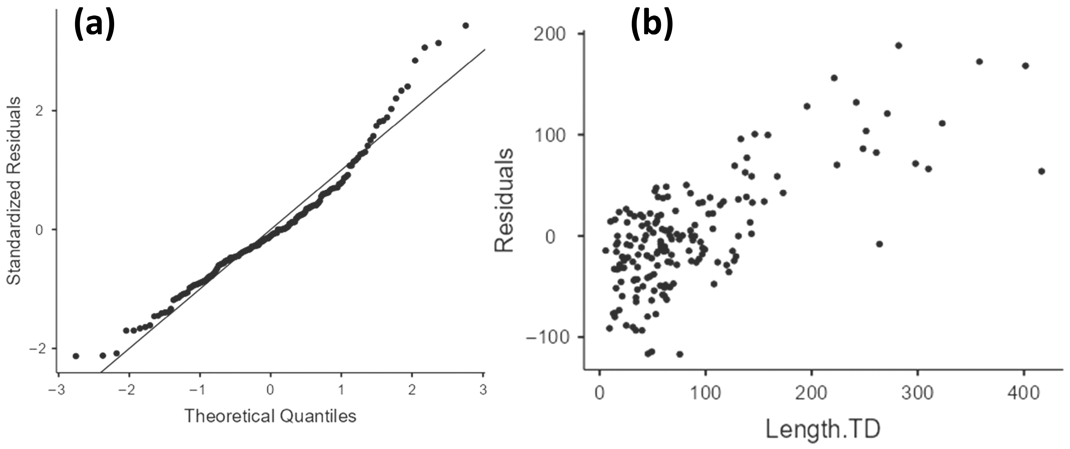
| Ac_CTD | 0.491 | 0.191 | 54.8 | 1.64 | 63 | 107 | 0.013 |
| Normality Tests | ||
|---|---|---|
| Tests | Statistic | p |
| Shapiro–Wilk | 0.959 | <0.001 |
| Heteroskedasticity Tests | ||
|---|---|---|
| Tests | Statistic | p |
| Breusch-Pagan | 65.3 | 0.397 |
| Durbin–Watson Test for Autocorrelation | ||
|---|---|---|
| Autocorrelation | DW Statistic | p |
| 0.142 | 1.71 | 0.038 |
| Collinearity Statistics | ||
|---|---|---|
| Predictor | VIF | Tolerance |
| D.LULC | 1.33 | 0.75 |
| D.SOIL | 2.8 | 0.357 |
| D.GEOU | 1.79 | 0.559 |
| D.Litho | 1.74 | 0.575 |
| D.ASP | 1.68 | 0.596 |
| D.PLCV | 2.14 | 0.467 |
| D.RNF | 2.78 | 0.36 |
| D.TPI | 1.7 | 0.589 |
| D.TWI | 2.99 | 0.335 |
| D.TRI | 2.31 | 0.433 |
| D.SDI | 2.34 | 0.427 |
| D.NDVI | 1.73 | 0.577 |
| D.LFDI | 3.66 | 0.273 |
| T.PLCV | 2.68 | 0.372 |
| T.TPI | 2.69 | 0.372 |
| T.Litho | 2.05 | 0.487 |
| T.SOIL | 1.61 | 0.622 |
| T.LULC | 1.6 | 0.624 |
| C.ASP | 1.78 | 0.561 |
| C.PLCV | 2.23 | 0.449 |
| C.RNF | 1.28 | 0.783 |
| C.TPI | 2.76 | 0.362 |
| C.TWI | 2.61 | 0.383 |
| C.TRI | 2.57 | 0.39 |
| C.LFDI | 3.48 | 0.288 |
| C.NDVI | 2.37 | 0.422 |
| C.NDBI | 2.22 | 0.45 |
| C.Litho | 1.47 | 0.679 |
| C.GEOU | 2.41 | 0.414 |
| C.SOIL | 3.09 | 0.323 |
| C.LULC | 1.51 | 0.664 |
| Area.C | 1.67 | 0.598 |
| Predictor | t | p | Stand. Estimate | 95% Confidence Interval | |
|---|---|---|---|---|---|
| Lower | Upper | ||||
| Intercept a | 0.1233 | 0.902 | |||
| D.LULC: | |||||
| Mosaic of Uses—Forest Formation | 0.9479 | 0.345 | 0.34734 | −0.3791 | 1.0738 |
| Pasture—Forest Formation | −0.5751 | 0.566 | −0.24047 | −1.0694 | 0.5884 |
| Rocky Outcrop—Forest Formation | −1.4733 | 0.144 | −1.53207 | −3.5935 | 0.5293 |
| Urban Area—Forest Formation | −1.0471 | 0.297 | −0.22668 | −0.6558 | 0.2025 |
| D.SOIL: | |||||
| CXbd4—AR3 | 1.0397 | 0.301 | 1.30479 | −1.1831 | 3.7927 |
| CXbd6—AR3 | 2.9863 | 0.004 | 1.74843 | 0.5878 | 2.9091 |
| LVAd24—AR3 | 2.1574 | 0.033 | 1.34981 | 0.1095 | 2.5901 |
| Urban area—AR3 | 3.2996 | 0.001 | 1.72437 | 0.6884 | 2.7604 |
| D.GEOU: | |||||
| Colluvial-talus slopes—Alluvial-colluvial slopes | −0.0523 | 0.958 | −0.02937 | −1.1416 | 1.0829 |
| Dissected hills and low hills—Alluvial-colluvial slopes | −0.5235 | 0.602 | −0.32065 | −1.535 | 0.8937 |
| Floodplains—Alluvial-colluvial slopes | 0.3131 | 0.755 | 0.21949 | −1.1702 | 1.6091 |
| High hills domain—Alluvial-colluvial slopes | −0.7418 | 0.46 | −0.38199 | −1.4028 | 0.6388 |
| Mountainous Domain—Alluvial-colluvial slopes | 0.1717 | 0.864 | 0.10754 | −1.1345 | 1.3496 |
| Mountainous escarpments—Alluvial-colluvial slopes | 0.0138 | 0.989 | 0.00989 | −1.4103 | 1.43 |
| D.Litho: | |||||
| NP3_gamma_1rnb—NP23_gamma_1rn | −1.5308 | 0.129 | −0.55078 | −1.264 | 0.1625 |
| NP3_gamma_3so—NP23_gamma_1rn | −1.233 | 0.22 | −0.75242 | −1.9621 | 0.4573 |
| NP3_gamma_3sor—NP23_gamma_1rn | 0.2908 | 0.772 | 0.32577 | −1.895 | 2.5465 |
| O1_gamma_6nfan—NP23_gamma_1rn | −1.1506 | 0.252 | −1.79314 | −4.8825 | 1.2962 |
| D.ASP | −0.1413 | 0.888 | −0.01635 | −0.2457 | 0.213 |
| D.PLCV | −0.0165 | 0.987 | −0.00244 | −0.2954 | 0.2906 |
| D.RNF | −0.3784 | 0.706 | −0.07256 | −0.4527 | 0.3076 |
| D.TPI | 1.3665 | 0.175 | 0.16011 | −0.0722 | 0.3924 |
| D.TWI | −0.1915 | 0.848 | −0.03949 | −0.4482 | 0.3693 |
| D.TRI | −0.822 | 0.413 | −0.13093 | −0.4467 | 0.1848 |
| D.SDI | 0.6101 | 0.543 | 0.09852 | −0.2216 | 0.4186 |
| D.NDVI | 0.6453 | 0.52 | 0.07722 | −0.16 | 0.3145 |
| D.LFDI | −1.8977 | 0.06 | −0.47971 | −0.9808 | 0.0214 |
| T.PLCV | 0.2517 | 0.802 | 0.04663 | −0.3206 | 0.4139 |
| T.TPI | −0.2784 | 0.781 | −0.0516 | −0.419 | 0.3158 |
| T.Litho: | |||||
| NP3_gamma_1rnb—NP23_gamma_1rn | 0.6983 | 0.486 | 0.26138 | −0.4806 | 1.0034 |
| NP3_gamma_3so—NP23_gamma_1rn | 1.2156 | 0.227 | 0.66209 | −0.4177 | 1.7418 |
| T.SOIL: | |||||
| CXbd4—AR3 | −0.9343 | 0.352 | −0.4267 | −1.332 | 0.4786 |
| CXbd6—AR3 | −0.302 | 0.763 | −0.13599 | −1.0287 | 0.7567 |
| LVAd24—AR3 | −1.6945 | 0.093 | −0.72744 | −1.5785 | 0.1236 |
| Urban area—AR3 | −0.4851 | 0.629 | −0.18348 | −0.9332 | 0.5663 |
| T.LULC: | |||||
| Mosaic of Uses—Forest Formation | −1.0772 | 0.284 | −0.31081 | −0.8828 | 0.2612 |
| Pasture—Forest Formation | 0.4108 | 0.682 | 0.19329 | −0.7394 | 1.126 |
| Rocky Outcrop—Forest Formation | −1.6909 | 0.094 | −1.5964 | −3.468 | 0.2752 |
| Urban Area—Forest Formation | 0.4514 | 0.653 | 0.1424 | −0.4829 | 0.7677 |
| C.ASP | 0.5385 | 0.591 | 0.06626 | −0.1776 | 0.3101 |
| C.PLCV | 0.5426 | 0.589 | 0.08335 | −0.2212 | 0.3879 |
| C.RNF | 0.8408 | 0.402 | 0.0741 | −0.1006 | 0.2488 |
| C.TPI | 1.35 | 0.18 | 0.25741 | −0.1206 | 0.6354 |
| C.TWI | 0.1722 | 0.864 | 0.031 | −0.3259 | 0.3879 |
| C.TRI | −0.7678 | 0.444 | −0.13592 | −0.4869 | 0.215 |
| C.LFDI | 1.7693 | 0.08 | 0.42451 | −0.0511 | 0.9001 |
| C.NDVI | 1.026 | 0.307 | 0.16775 | −0.1564 | 0.4919 |
| C.NDBI | 1.6316 | 0.106 | 0.24993 | −0.0537 | 0.5536 |
| C.Litho: | |||||
| NP3_gamma_1rnb—NP23_gamma_1rn | 0.0196 | 0.984 | 0.00485 | −0.4865 | 0.4962 |
| NP3_gamma_3so—NP23_gamma_1rn | −0.369 | 0.713 | −0.14954 | −0.9529 | 0.6538 |
| C.GEOU: | |||||
| Dissected hills and Low hills—Colluvial-Talus slopes | −0.1363 | 0.892 | −0.18638 | −2.8975 | 2.5248 |
| High mountainous domain—Colluvial-Talus slopes | −0.2348 | 0.815 | −0.27582 | −2.6044 | 2.0528 |
| Mountainous domain—Colluvial-Talus slopes | −0.1457 | 0.884 | −0.19044 | −2.7808 | 2.4 |
| Mountainous escarpments—Colluvial-Talus slopes | −0.3062 | 0.76 | −0.33562 | −2.5082 | 1.837 |
| C.SOIL: | |||||
| CXbd4—AR3 | −0.5388 | 0.591 | −0.65642 | −3.0716 | 1.7587 |
| CXbd6—AR3 | −2.307 | 0.023 | −1.2557 | −2.3347 | −0.1767 |
| LVAd24—AR3 | −1.7949 | 0.075 | −1.16457 | −2.4508 | 0.1216 |
| Urban area—AR3 | −2.4068 | 0.018 | −1.34458 | −2.4521 | −0.2371 |
| C.LULC: | |||||
| Mosaic of Uses—Forest Formation | −1.3528 | 0.179 | −0.3635 | −0.8962 | 0.1692 |
| Pasture—Forest Formation | −1.8654 | 0.065 | −0.74576 | −1.5383 | 0.0468 |
| Rocky Outcrop—Forest Formation | −1.5044 | 0.135 | −1.39298 | −3.2285 | 0.4425 |
| Urban Area—Forest Formation | −0.9351 | 0.352 | −0.29039 | −0.906 | 0.3253 |
| Area.C | 1.4465 | 0.151 | 0.16688 | −0.0618 | 0.3956 |
Appendix B.5. Vc0.5-CTD Model
| Model Fit Measures | Overall Model Test | ||||||
|---|---|---|---|---|---|---|---|
| Model | R2 | Adjusted R2 | RMSE | F | df1 | df2 | p |
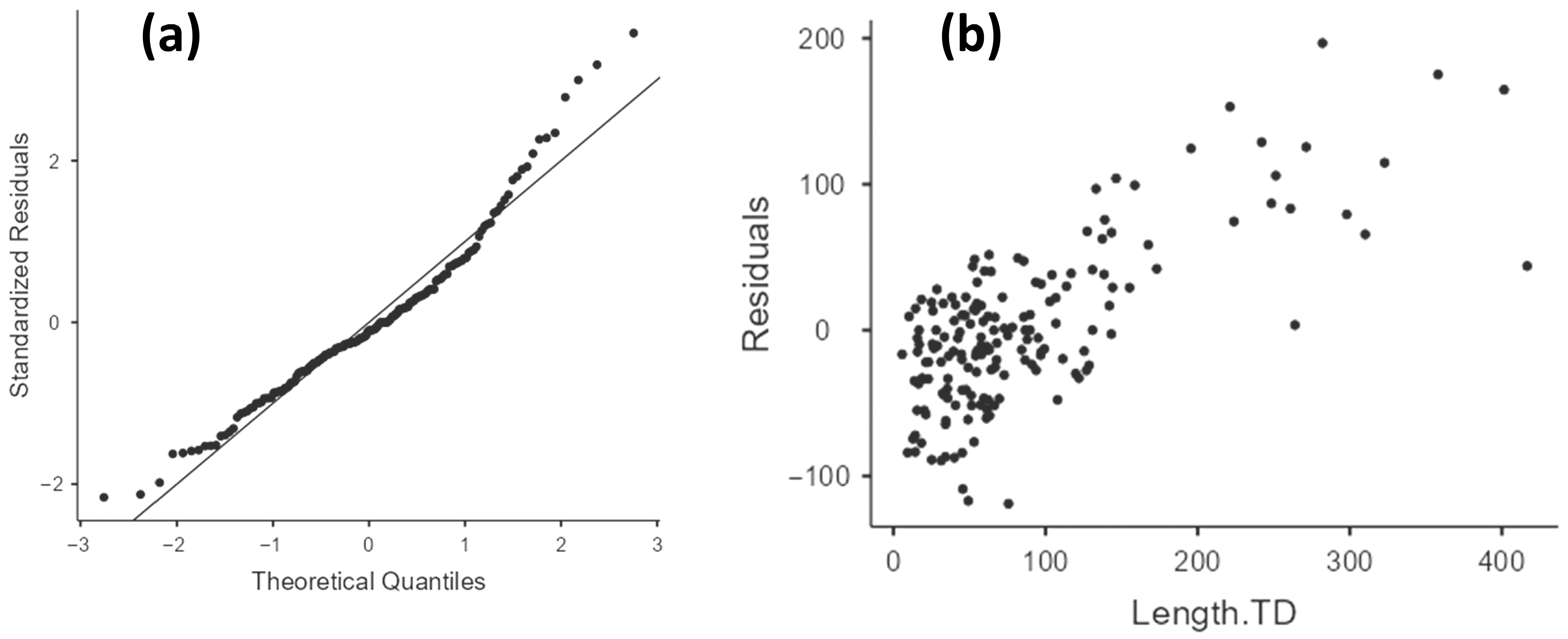
| Vc_CTD_0.5 | 0.49 | 0.189 | 54.8 | 1.63 | 63 | 107 | 0.013 |
| Normality Tests | ||
|---|---|---|
| Tests | Statistic | p |
| Shapiro–Wilk | 0.957 | <0.001 |
| Heteroskedasticity Tests | ||
|---|---|---|
| Tests | Statistic | p |
| Breusch–Pagan | 65.4 | 0.392 |
| Durbin–Watson Test for Autocorrelation | ||
|---|---|---|
| Autocorrelation | DW Statistic | p |
| 0.144 | 1.71 | 0.06 |
| Collinearity Statistics | ||
|---|---|---|
| Predictor | VIF | Tolerance |
| D.LULC | 1.34 | 0.749 |
| D.SOIL | 2.82 | 0.354 |
| D.GEOU | 1.79 | 0.558 |
| D.Litho | 1.74 | 0.575 |
| D.ASP | 1.69 | 0.59 |
| D.PLCV | 2.15 | 0.466 |
| D.RNF | 2.77 | 0.361 |
| D.TPI | 1.7 | 0.589 |
| D.TWI | 2.99 | 0.334 |
| D.TRI | 2.29 | 0.436 |
| D.SDI | 2.34 | 0.428 |
| D.NDVI | 1.72 | 0.58 |
| D.LFDI | 3.72 | 0.269 |
| T.PLCV | 2.65 | 0.377 |
| T.TPI | 2.71 | 0.37 |
| T.Litho | 2.05 | 0.488 |
| T.SOIL | 1.61 | 0.62 |
| T.LULC | 1.6 | 0.624 |
| C.ASP | 1.81 | 0.551 |
| C.PLCV | 2.19 | 0.456 |
| C.RNF | 1.28 | 0.783 |
| C.TPI | 2.82 | 0.354 |
| C.TWI | 2.61 | 0.383 |
| C.TRI | 2.54 | 0.394 |
| C.LFDI | 3.52 | 0.284 |
| C.NDVI | 2.36 | 0.423 |
| C.NDBI | 2.22 | 0.449 |
| C.Litho | 1.47 | 0.68 |
| C.GEOU | 2.41 | 0.414 |
| C.SOIL | 3.12 | 0.321 |
| C.LULC | 1.49 | 0.669 |
| Vol.C_0.5 | 1.58 | 0.634 |
| Predictor | t | p | Stand. Estimate | 95% Confidence Interval | |
|---|---|---|---|---|---|
| Lower | Upper | ||||
| Intercept a | 0.08533 | 0.932 | |||
| D.LULC: | |||||
| Mosaic of Uses—Forest Formation | 0.93821 | 0.35 | 0.34408 | −0.3829 | 1.0711 |
| Pasture—Forest Formation | −0.69754 | 0.487 | −0.29354 | −1.1278 | 0.5407 |
| Rocky Outcrop—Forest Formation | −1.51157 | 0.134 | −1.57327 | −3.6366 | 0.49 |
| Urban Area—Forest Formation | −1.07437 | 0.285 | −0.23263 | −0.6619 | 0.1966 |
| D.SOIL: | |||||
| CXbd4—AR3 | 0.97312 | 0.333 | 1.21867 | −1.2639 | 3.7013 |
| CXbd6—AR3 | 2.69395 | 0.008 | 1.62045 | 0.428 | 2.8129 |
| LVAd24—AR3 | 2.05507 | 0.042 | 1.28926 | 0.0456 | 2.5329 |
| Urban area—AR3 | 3.10907 | 0.002 | 1.64232 | 0.5952 | 2.6895 |
| D.GEOU: | |||||
| Colluvial-talus slopes—Alluvial-colluvial slopes | −0.07836 | 0.938 | −0.04412 | −1.1601 | 1.0719 |
| Dissected hills and low hills—Alluvial-colluvial slopes | −0.58056 | 0.563 | −0.35812 | −1.5809 | 0.8647 |
| Floodplains—Alluvial-colluvial slopes | 0.33115 | 0.741 | 0.23223 | −1.158 | 1.6224 |
| High hills domain—Alluvial-colluvial slopes | −0.74339 | 0.459 | −0.38403 | −1.4081 | 0.6401 |
| Mountainous Domain—Alluvial-colluvial slopes | 0.18673 | 0.852 | 0.11719 | −1.1269 | 1.3613 |
| Mountainous escarpments—Alluvial-colluvial slopes | 0.00584 | 0.995 | 0.00419 | −1.4178 | 1.4261 |
| D.Litho: | |||||
| NP3_gamma_1rnb—NP23_gamma_1rn | −1.48474 | 0.141 | −0.53508 | −1.2495 | 0.1793 |
| NP3_gamma_3so—NP23_gamma_1rn | −1.13497 | 0.259 | −0.69318 | −1.9039 | 0.5176 |
| NP3_gamma_3sor—NP23_gamma_1rn | 0.24369 | 0.808 | 0.27328 | −1.9498 | 2.4964 |
| O1_gamma_6nfan—NP23_gamma_1rn | −1.12441 | 0.263 | −1.75407 | −4.8466 | 1.3384 |
| D.ASP | −0.2474 | 0.805 | −0.02896 | −0.261 | 0.2031 |
| D.PLCV | −0.02453 | 0.98 | −0.00363 | −0.2973 | 0.2901 |
| D.RNF | −0.33644 | 0.737 | −0.06444 | −0.4442 | 0.3153 |
| D.TPI | 1.33513 | 0.185 | 0.15667 | −0.0759 | 0.3893 |
| D.TWI | −0.1898 | 0.85 | −0.0392 | −0.4487 | 0.3703 |
| D.TRI | −0.90253 | 0.369 | −0.14282 | −0.4565 | 0.1709 |
| D.SDI | 0.53555 | 0.593 | 0.08648 | −0.2336 | 0.4066 |
| D.NDVI | 0.58893 | 0.557 | 0.07013 | −0.1659 | 0.3062 |
| D.LFDI | −1.75232 | 0.083 | −0.44995 | −0.959 | 0.0591 |
| T.PLCV | 0.12291 | 0.902 | 0.02249 | −0.3403 | 0.3853 |
| T.TPI | −0.19139 | 0.849 | −0.03577 | −0.4063 | 0.3347 |
| T.Litho: | |||||
| NP3_gamma_1rnb—NP23_gamma_1rn | 0.62936 | 0.53 | 0.23562 | −0.5065 | 0.9778 |
| NP3_gamma_3so—NP23_gamma_1rn | 1.1838 | 0.239 | 0.64445 | −0.4347 | 1.7236 |
| T.SOIL: | |||||
| CXbd4—AR3 | −1.03472 | 0.303 | −0.47449 | −1.3835 | 0.4346 |
| CXbd6—AR3 | −0.42022 | 0.675 | −0.19111 | −1.0927 | 0.7105 |
| LVAd24—AR3 | −1.81213 | 0.073 | −0.78 | −1.6333 | 0.0733 |
| Urban area—AR3 | −0.55866 | 0.578 | −0.21141 | −0.9616 | 0.5388 |
| T.LULC: | |||||
| Mosaic of Uses—Forest Formation | −1.22781 | 0.222 | −0.35363 | −0.9246 | 0.2173 |
| Pasture—Forest Formation | 0.32761 | 0.744 | 0.15359 | −0.7758 | 1.083 |
| Rocky Outcrop—Forest Formation | −1.56081 | 0.122 | −1.48048 | −3.3608 | 0.3999 |
| Urban Area—Forest Formation | 0.42573 | 0.671 | 0.13432 | −0.4911 | 0.7598 |
| C.ASP | 0.6726 | 0.503 | 0.0843 | −0.1642 | 0.3327 |
| C.PLCV | 0.76878 | 0.444 | 0.11647 | −0.1839 | 0.4168 |
| C.RNF | 0.85973 | 0.392 | 0.07579 | −0.099 | 0.2505 |
| C.TPI | 1.22295 | 0.224 | 0.23845 | −0.1481 | 0.625 |
| C.TWI | 0.19429 | 0.846 | 0.035 | −0.3222 | 0.3922 |
| C.TRI | −0.65851 | 0.512 | −0.11549 | −0.4632 | 0.2322 |
| C.LFDI | 1.64314 | 0.103 | 0.39947 | −0.0825 | 0.8814 |
| C.NDVI | 0.99139 | 0.324 | 0.1618 | −0.1617 | 0.4853 |
| C.NDBI | 1.57065 | 0.119 | 0.24133 | −0.0633 | 0.5459 |
| C.Litho: | |||||
| NP3_gamma_1rnb—NP23_gamma_1rn | 0.08077 | 0.936 | 0.02005 | −0.472 | 0.512 |
| NP3_gamma_3so—NP23_gamma_1rn | −0.34007 | 0.734 | −0.13779 | −0.941 | 0.6654 |
| C.GEOU: | |||||
| Dissected hills and Low hills—Colluvial-Talus slopes | −0.13044 | 0.896 | −0.17854 | −2.892 | 2.5349 |
| High mountainous domain—Colluvial-Talus slopes | −0.23957 | 0.811 | −0.28173 | −2.613 | 2.0495 |
| Mountainous domain—Colluvial-Talus slopes | −0.20321 | 0.839 | −0.26614 | −2.8625 | 2.3302 |
| Mountainous escarpments—Colluvial-Talus slopes | −0.29715 | 0.767 | −0.3259 | −2.5001 | 1.8483 |
| C.SOIL: | |||||
| CXbd4—AR3 | −0.50791 | 0.613 | −0.61932 | −3.0365 | 1.7979 |
| CXbd6—AR3 | −1.95323 | 0.053 | −1.11039 | −2.2374 | 0.0166 |
| LVAd24—AR3 | −1.69246 | 0.093 | −1.10905 | −2.4081 | 0.19 |
| Urban area—AR3 | −2.30688 | 0.023 | −1.30916 | −2.4342 | −0.1842 |
| C.LULC: | |||||
| Mosaic of Uses—Forest Formation | −1.20935 | 0.229 | −0.32209 | −0.8501 | 0.2059 |
| Pasture—Forest Formation | −1.72853 | 0.087 | −0.68211 | −1.4644 | 0.1002 |
| Rocky Outcrop—Forest Formation | −1.37844 | 0.171 | −1.26913 | −3.0943 | 0.5561 |
| Urban Area—Forest Formation | −0.96261 | 0.338 | −0.29899 | −0.9147 | 0.3167 |
| Vol.C.0.5 | 1.37511 | 0.172 | 0.14975 | −0.0661 | 0.3656 |
Appendix B.6. Vc1.0-CTD Model
| Model Fit Measures | Overall Model Test | ||||||
|---|---|---|---|---|---|---|---|
| Model | R2 | Adjusted R2 | RMSE | F | df1 | df2 | p |
| Vc_CTD_1.0 | 0.49 | 0.189 | 54.8 | 1.63 | 63 | 107 | 0.013 |
| Normality Tests | ||
|---|---|---|
| Tests | Statistic | p |
| Shapiro-Wilk | 0.957 | <0.001 |
| Heteroskedasticity Tests | ||
|---|---|---|
| Tests | Statistic | p |
| Breusch-Pagan | 65.4 | 0.392 |
| Durbin–Watson Test for Autocorrelation | ||
|---|---|---|
| Autocorrelation | DW Statistic | p |
| 0.144 | 1.71 | 0.058 |
| Collinearity Statistics | ||
|---|---|---|
| Predictor | VIF | Tolerance |
| D.LULC | 1.34 | 0.749 |
| D.SOIL | 2.82 | 0.354 |
| D.GEOU | 1.79 | 0.558 |
| D.Litho | 1.74 | 0.575 |
| D.ASP | 1.69 | 0.59 |
| D.PLCV | 2.15 | 0.466 |
| D.RNF | 2.77 | 0.361 |
| D.TPI | 1.7 | 0.589 |
| D.TWI | 2.99 | 0.334 |
| D.TRI | 2.29 | 0.436 |
| D.SDI | 2.34 | 0.428 |
| D.NDVI | 1.72 | 0.58 |
| D.LFDI | 3.72 | 0.269 |
| T.PLCV | 2.65 | 0.377 |
| T.TPI | 2.71 | 0.37 |
| T.Litho | 2.05 | 0.488 |
| T.SOIL | 1.61 | 0.62 |
| T.LULC | 1.6 | 0.624 |
| C.ASP | 1.81 | 0.551 |
| C.PLCV | 2.19 | 0.456 |
| C.RNF | 1.28 | 0.783 |
| C.TPI | 2.82 | 0.354 |
| C.TWI | 2.61 | 0.383 |
| C.TRI | 2.54 | 0.394 |
| C.LFDI | 3.52 | 0.284 |
| C.NDVI | 2.36 | 0.423 |
| C.NDBI | 2.22 | 0.449 |
| C.Litho | 1.47 | 0.68 |
| C.GEOU | 2.41 | 0.414 |
| C.SOIL | 3.12 | 0.321 |
| C.LULC | 1.49 | 0.669 |
| Volume collapse (1.0) | 1.58 | 0.634 |
| Predictor | t | p | Stand. Estimate | 95% Confidence Interval | |
|---|---|---|---|---|---|
| Lower | Upper | ||||
| Intercept a | 0.08533 | 0.932 | |||
| D.LULC: | |||||
| Mosaic of Uses—Forest Formation | 0.93821 | 0.35 | 0.34408 | −0.3829 | 1.0711 |
| Pasture—Forest Formation | −0.69754 | 0.487 | −0.29354 | −1.1278 | 0.5407 |
| Rocky Outcrop—Forest Formation | −1.51157 | 0.134 | −1.57327 | −3.6366 | 0.49 |
| Urban Area—Forest Formation | −1.07437 | 0.285 | −0.23263 | −0.6619 | 0.1966 |
| D.SOIL: | |||||
| CXbd4—AR3 | 0.97312 | 0.333 | 1.21867 | −1.2639 | 3.7013 |
| CXbd6—AR3 | 2.69395 | 0.008 | 1.62045 | 0.428 | 2.8129 |
| LVAd24—AR3 | 2.05507 | 0.042 | 1.28926 | 0.0456 | 2.5329 |
| Urban area—AR3 | 3.10907 | 0.002 | 1.64232 | 0.5952 | 2.6895 |
| D.GEOU: | |||||
| Colluvial-talus slopes—Alluvial-colluvial slopes | −0.07836 | 0.938 | −0.04412 | −1.1601 | 1.0719 |
| Dissected hills and low hills—Alluvial-colluvial slopes | −0.58056 | 0.563 | −0.35812 | −1.5809 | 0.8647 |
| Floodplains—Alluvial-colluvial slopes | 0.33115 | 0.741 | 0.23223 | −1.158 | 1.6224 |
| High hills domain—Alluvial-colluvial slopes | −0.74339 | 0.459 | −0.38403 | −1.4081 | 0.6401 |
| Mountainous Domain—Alluvial-colluvial slopes | 0.18673 | 0.852 | 0.11719 | −1.1269 | 1.3613 |
| Mountainous escarpments—Alluvial-colluvial slopes | 0.00584 | 0.995 | 0.00419 | −1.4178 | 1.4261 |
| D.Litho: | |||||
| NP3_gamma_1rnb—NP23_gamma_1rn | −1.48474 | 0.141 | −0.53508 | −1.2495 | 0.1793 |
| NP3_gamma_3so—NP23_gamma_1rn | −1.13497 | 0.259 | −0.69318 | −1.9039 | 0.5176 |
| NP3_gamma_3sor—NP23_gamma_1rn | 0.24369 | 0.808 | 0.27328 | −1.9498 | 2.4964 |
| O1_gamma_6nfan—NP23_gamma_1rn | −1.12441 | 0.263 | −1.75407 | −4.8466 | 1.3384 |
| D.ASP | −0.2474 | 0.805 | −0.02896 | −0.261 | 0.2031 |
| D.PLCV | −0.02453 | 0.98 | −0.00363 | −0.2973 | 0.2901 |
| D.RNF | −0.33644 | 0.737 | −0.06444 | −0.4442 | 0.3153 |
| D.TPI | 1.33513 | 0.185 | 0.15667 | −0.0759 | 0.3893 |
| D.TWI | −0.1898 | 0.85 | −0.0392 | −0.4487 | 0.3703 |
| D.TRI | −0.90253 | 0.369 | −0.14282 | −0.4565 | 0.1709 |
| D.SDI | 0.53555 | 0.593 | 0.08648 | −0.2336 | 0.4066 |
| D.NDVI | 0.58893 | 0.557 | 0.07013 | −0.1659 | 0.3062 |
| D.LFDI | −1.75232 | 0.083 | −0.44995 | −0.959 | 0.0591 |
| T.PLCV | 0.12291 | 0.902 | 0.02249 | −0.3403 | 0.3853 |
| T.TPI | −0.19139 | 0.849 | −0.03577 | −0.4063 | 0.3347 |
| T.Litho: | |||||
| NP3_gamma_1rnb—NP23_gamma_1rn | 0.62936 | 0.53 | 0.23562 | −0.5065 | 0.9778 |
| NP3_gamma_3so—NP23_gamma_1rn | 1.1838 | 0.239 | 0.64445 | −0.4347 | 1.7236 |
| T.SOIL: | |||||
| CXbd4—AR3 | −1.03472 | 0.303 | −0.47449 | −1.3835 | 0.4346 |
| CXbd6—AR3 | −0.42022 | 0.675 | −0.19111 | −1.0927 | 0.7105 |
| LVAd24—AR3 | −1.81213 | 0.073 | −0.78 | −1.6333 | 0.0733 |
| Urban area—AR3 | −0.55866 | 0.578 | −0.21141 | −0.9616 | 0.5388 |
| T.LULC: | |||||
| Mosaic of Uses—Forest Formation | −1.22781 | 0.222 | −0.35363 | −0.9246 | 0.2173 |
| Pasture—Forest Formation | 0.32761 | 0.744 | 0.15359 | −0.7758 | 1.083 |
| Rocky Outcrop—Forest Formation | −1.56081 | 0.122 | −1.48048 | −3.3608 | 0.3999 |
| Urban Area—Forest Formation | 0.42573 | 0.671 | 0.13432 | −0.4911 | 0.7598 |
| C.ASP | 0.6726 | 0.503 | 0.0843 | −0.1642 | 0.3327 |
| C.PLCV | 0.76878 | 0.444 | 0.11647 | −0.1839 | 0.4168 |
| C.RNF | 0.85973 | 0.392 | 0.07579 | −0.099 | 0.2505 |
| C.TPI | 1.22295 | 0.224 | 0.23845 | −0.1481 | 0.625 |
| C.TWI | 0.19429 | 0.846 | 0.035 | −0.3222 | 0.3922 |
| C.TRI | −0.65851 | 0.512 | −0.11549 | −0.4632 | 0.2322 |
| C.LFDI | 1.64314 | 0.103 | 0.39947 | −0.0825 | 0.8814 |
| C.NDVI | 0.99139 | 0.324 | 0.1618 | −0.1617 | 0.4853 |
| C.NDBI | 1.57065 | 0.119 | 0.24133 | −0.0633 | 0.5459 |
| C.Litho: | |||||
| NP3_gamma_1rnb—NP23_gamma_1rn | 0.08077 | 0.936 | 0.02005 | −0.472 | 0.512 |
| NP3_gamma_3so—NP23_gamma_1rn | −0.34007 | 0.734 | −0.13779 | −0.941 | 0.6654 |
| C.GEOU: | |||||
| Dissected hills and Low hills—Colluvial-Talus slopes | −0.13044 | 0.896 | −0.17854 | −2.892 | 2.5349 |
| High mountainous domain—Colluvial-Talus slopes | −0.23957 | 0.811 | −0.28173 | −2.613 | 2.0495 |
| Mountainous domain—Colluvial-Talus slopes | −0.20321 | 0.839 | −0.26614 | −2.8625 | 2.3302 |
| Mountainous escarpments—Colluvial-Talus slopes | −0.29715 | 0.767 | −0.3259 | −2.5001 | 1.8483 |
| C.SOIL: | |||||
| CXbd4—AR3 | −0.50791 | 0.613 | −0.61932 | −3.0365 | 1.7979 |
| CXbd6—AR3 | −1.95323 | 0.053 | −1.11039 | −2.2374 | 0.0166 |
| LVAd24—AR3 | −1.69246 | 0.093 | −1.10905 | −2.4081 | 0.19 |
| Urban area—AR3 | −2.30688 | 0.023 | −1.30916 | −2.4342 | −0.1842 |
| C.LULC: | |||||
| Mosaic of Uses—Forest Formation | −1.20935 | 0.229 | −0.32209 | −0.8501 | 0.2059 |
| Pasture—Forest Formation | −1.72853 | 0.087 | −0.68211 | −1.4644 | 0.1002 |
| Rocky Outcrop—Forest Formation | −1.37844 | 0.171 | −1.26913 | −3.0943 | 0.5561 |
| Urban Area—Forest Formation | −0.96261 | 0.338 | −0.29899 | −0.9147 | 0.3167 |
| Volume collapse (1.0) | 1.37511 | 0.172 | 0.14975 | −0.0661 | 0.3656 |

Appendix B.7. Vc1.5-CTD Model
| Model Fit Measures | Overall Model Test | ||||||
|---|---|---|---|---|---|---|---|
| Model | R2 | Adjusted R2 | RMSE | F | df1 | df2 | p |
| Vc_CTD_1.5 | 0.49 | 0.189 | 54.8 | 1.63 | 63 | 107 | 0.013 |
| Normality Tests | ||
|---|---|---|
| Tests | Statistic | p |
| Shapiro–Wilk | 0.957 | <0.001 |
| Heteroskedasticity Tests | ||
|---|---|---|
| Tests | Statistic | p |
| Breusch-Pagan | 65.4 | 0.392 |
| Durbin–Watson Test for Autocorrelation | ||
|---|---|---|
| Autocorrelation | DW Statistic | p |
| 0.144 | 1.71 | 0.044 |
| Collinearity Statistics | ||
|---|---|---|
| Predictor | VIF | Tolerance |
| D.LULC | 1.34 | 0.749 |
| D.SOIL | 2.82 | 0.354 |
| D.GEOU | 1.79 | 0.558 |
| D.Litho | 1.74 | 0.575 |
| D.ASP | 1.69 | 0.59 |
| D.PLCV | 2.15 | 0.466 |
| D.RNF | 2.77 | 0.361 |
| D.TPI | 1.7 | 0.589 |
| D.TWI | 2.99 | 0.334 |
| D.TRI | 2.29 | 0.436 |
| D.SDI | 2.34 | 0.428 |
| D.NDVI | 1.72 | 0.58 |
| D.LFDI | 3.72 | 0.269 |
| T.PLCV | 2.65 | 0.377 |
| T.TPI | 2.71 | 0.37 |
| T.Litho | 2.05 | 0.488 |
| T.SOIL | 1.61 | 0.62 |
| T.LULC | 1.6 | 0.624 |
| C.ASP | 1.81 | 0.551 |
| C.PLCV | 2.19 | 0.456 |
| C.RNF | 1.28 | 0.783 |
| C.TPI | 2.82 | 0.354 |
| C.TWI | 2.61 | 0.383 |
| C.TRI | 2.54 | 0.394 |
| C.LFDI | 3.52 | 0.284 |
| C.NDVI | 2.36 | 0.423 |
| C.NDBI | 2.22 | 0.449 |
| C.Litho | 1.47 | 0.68 |
| C.GEOU | 2.41 | 0.414 |
| C.SOIL | 3.12 | 0.321 |
| C.LULC | 1.49 | 0.669 |
| Vol.C_1.5 | 1.58 | 0.634 |
| Predictor | t | p | Stand. Estimate | 95% Confidence Interval | |
|---|---|---|---|---|---|
| Lower | Upper | ||||
| Intercept a | 0.08533 | 0.932 | |||
| D.LULC: | |||||
| Mosaic of Uses—Forest Formation | 0.93821 | 0.35 | 0.34408 | −0.3829 | 1.0711 |
| Pasture—Forest Formation | −0.69754 | 0.487 | −0.29354 | −1.1278 | 0.5407 |
| Rocky Outcrop—Forest Formation | −1.51157 | 0.134 | −1.57327 | −3.6366 | 0.49 |
| Urban Area—Forest Formation | −1.07437 | 0.285 | −0.23263 | −0.6619 | 0.1966 |
| D.SOIL: | |||||
| CXbd4—AR3 | 0.97312 | 0.333 | 1.21867 | −1.2639 | 3.7013 |
| CXbd6—AR3 | 2.69395 | 0.008 | 1.62045 | 0.428 | 2.8129 |
| LVAd24—AR3 | 2.05507 | 0.042 | 1.28926 | 0.0456 | 2.5329 |
| Urban area—AR3 | 3.10907 | 0.002 | 1.64232 | 0.5952 | 2.6895 |
| D.GEOU: | |||||
| Colluvial-talus slopes—Alluvial-colluvial slopes | −0.07836 | 0.938 | −0.04412 | −1.1601 | 1.0719 |
| Dissected hills and low hills—Alluvial-colluvial slopes | −0.58056 | 0.563 | −0.35812 | −1.5809 | 0.8647 |
| Floodplains—Alluvial-colluvial slopes | 0.33115 | 0.741 | 0.23223 | −1.158 | 1.6224 |
| High hills domain—Alluvial-colluvial slopes | −0.74339 | 0.459 | −0.38403 | −1.4081 | 0.6401 |
| Mountainous Domain—Alluvial-colluvial slopes | 0.18673 | 0.852 | 0.11719 | −1.1269 | 1.3613 |
| Mountainous escarpments—Alluvial-colluvial slopes | 0.00584 | 0.995 | 0.00419 | −1.4178 | 1.4261 |
| D.Litho: | |||||
| NP3_gamma_1rnb—NP23_gamma_1rn | −1.48474 | 0.141 | −0.53508 | −1.2495 | 0.1793 |
| NP3_gamma_3so—NP23_gamma_1rn | −1.13497 | 0.259 | −0.69318 | −1.9039 | 0.5176 |
| NP3_gamma_3sor—NP23_gamma_1rn | 0.24369 | 0.808 | 0.27328 | −1.9498 | 2.4964 |
| O1_gamma_6nfan—NP23_gamma_1rn | −1.12441 | 0.263 | −1.75407 | −4.8466 | 1.3384 |
| D.ASP | −0.2474 | 0.805 | −0.02896 | −0.261 | 0.2031 |
| D.PLCV | −0.02453 | 0.98 | −0.00363 | −0.2973 | 0.2901 |
| D.RNF | −0.33644 | 0.737 | −0.06444 | −0.4442 | 0.3153 |
| D.TPI | 1.33513 | 0.185 | 0.15667 | −0.0759 | 0.3893 |
| D.TWI | −0.1898 | 0.85 | −0.0392 | −0.4487 | 0.3703 |
| D.TRI | −0.90253 | 0.369 | −0.14282 | −0.4565 | 0.1709 |
| D.SDI | 0.53555 | 0.593 | 0.08648 | −0.2336 | 0.4066 |
| D.NDVI | 0.58893 | 0.557 | 0.07013 | −0.1659 | 0.3062 |
| D.LFDI | −1.75232 | 0.083 | −0.44995 | −0.959 | 0.0591 |
| T.PLCV | 0.12291 | 0.902 | 0.02249 | −0.3403 | 0.3853 |
| T.TPI | −0.19139 | 0.849 | −0.03577 | −0.4063 | 0.3347 |
| T.Litho: | |||||
| NP3_gamma_1rnb—NP23_gamma_1rn | 0.62936 | 0.53 | 0.23562 | −0.5065 | 0.9778 |
| NP3_gamma_3so—NP23_gamma_1rn | 1.1838 | 0.239 | 0.64445 | −0.4347 | 1.7236 |
| T.SOIL: | |||||
| CXbd4—AR3 | −1.03472 | 0.303 | −0.47449 | −1.3835 | 0.4346 |
| CXbd6—AR3 | −0.42022 | 0.675 | −0.19111 | −1.0927 | 0.7105 |
| LVAd24—AR3 | −1.81213 | 0.073 | −0.78 | −1.6333 | 0.0733 |
| Urban area—AR3 | −0.55866 | 0.578 | −0.21141 | −0.9616 | 0.5388 |
| T.LULC: | |||||
| Mosaic of Uses—Forest Formation | −1.22781 | 0.222 | −0.35363 | −0.9246 | 0.2173 |
| Pasture—Forest Formation | 0.32761 | 0.744 | 0.15359 | −0.7758 | 1.083 |
| Rocky Outcrop—Forest Formation | −1.56081 | 0.122 | −1.48048 | −3.3608 | 0.3999 |
| Urban Area—Forest Formation | 0.42573 | 0.671 | 0.13432 | −0.4911 | 0.7598 |
| C.ASP | 0.6726 | 0.503 | 0.0843 | −0.1642 | 0.3327 |
| C.PLCV | 0.76878 | 0.444 | 0.11647 | −0.1839 | 0.4168 |
| C.RNF | 0.85973 | 0.392 | 0.07579 | −0.099 | 0.2505 |
| C.TPI | 1.22295 | 0.224 | 0.23845 | −0.1481 | 0.625 |
| C.TWI | 0.19429 | 0.846 | 0.035 | −0.3222 | 0.3922 |
| C.TRI | −0.65851 | 0.512 | −0.11549 | −0.4632 | 0.2322 |
| C.LFDI | 1.64314 | 0.103 | 0.39947 | −0.0825 | 0.8814 |
| C.NDVI | 0.99139 | 0.324 | 0.1618 | −0.1617 | 0.4853 |
| C.NDBI | 1.57065 | 0.119 | 0.24133 | −0.0633 | 0.5459 |
| C.Litho: | |||||
| NP3_gamma_1rnb—NP23_gamma_1rn | 0.08077 | 0.936 | 0.02005 | −0.472 | 0.512 |
| NP3_gamma_3so—NP23_gamma_1rn | −0.34007 | 0.734 | −0.13779 | −0.941 | 0.6654 |
| C.GEOU: | |||||
| Dissected hills and Low hills—Colluvial-Talus slopes | −0.13044 | 0.896 | −0.17854 | −2.892 | 2.5349 |
| High mountainous domain—Colluvial-Talus slopes | −0.23957 | 0.811 | −0.28173 | −2.613 | 2.0495 |
| Mountainous domain—Colluvial-Talus slopes | −0.20321 | 0.839 | −0.26614 | −2.8625 | 2.3302 |
| Mountainous escarpments—Colluvial-Talus slopes | −0.29715 | 0.767 | −0.3259 | −2.5001 | 1.8483 |
| C.SOIL: | |||||
| CXbd4—AR3 | −0.50791 | 0.613 | −0.61932 | −3.0365 | 1.7979 |
| CXbd6—AR3 | −1.95323 | 0.053 | −1.11039 | −2.2374 | 0.0166 |
| LVAd24—AR3 | −1.69246 | 0.093 | −1.10905 | −2.4081 | 0.19 |
| Urban area—AR3 | −2.30688 | 0.023 | −1.30916 | −2.4342 | −0.1842 |
| C.LULC: | |||||
| Mosaic of Uses—Forest Formation | −1.20935 | 0.229 | −0.32209 | −0.8501 | 0.2059 |
| Pasture—Forest Formation | −1.72853 | 0.087 | −0.68211 | −1.4644 | 0.1002 |
| Rocky Outcrop—Forest Formation | −1.37844 | 0.171 | −1.26913 | −3.0943 | 0.5561 |
| Urban Area—Forest Formation | −0.96261 | 0.338 | −0.29899 | −0.9147 | 0.3167 |
| Vol.C_1.5 | 1.37511 | 0.172 | 0.14975 | −0.0661 | 0.3656 |

Appendix B.8. Log10Ac-CTD Model
| Model Fit Measures | Overall Model Test | ||||||
|---|---|---|---|---|---|---|---|
| Model | R2 | Adjusted R2 | RMSE | F | df1 | df2 | p |
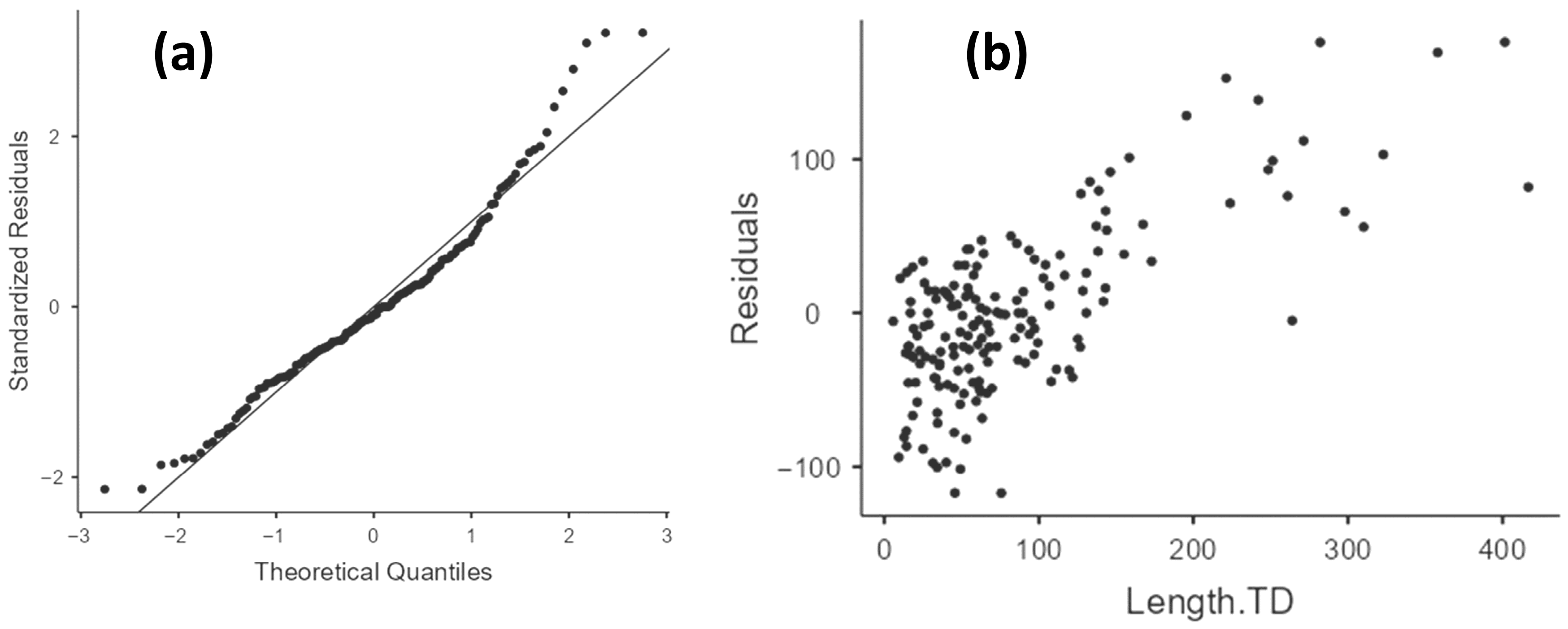
| LogAc_CTD | 0.495 | 0.197 | 54.5 | 1.66 | 63 | 107 | 0.01 |
| Normality Tests | ||
|---|---|---|
| Tests | Statistic | p |
| Shapiro-Wilk | 0.963 | <0.001 |
| Heteroskedasticity Tests | ||
|---|---|---|
| Tests | Statistic | p |
| Breusch–Pagan | 68.3 | 0.303 |
| Durbin–Watson Test for Autocorrelation | ||
|---|---|---|
| Autocorrelation | DW Statistic | p |
| 0.153 | 1.68 | 0.03 |
| Collinearity Statistics | ||
|---|---|---|
| Predictor | VIF | Tolerance |
| D.LULC | 1.34 | 0.749 |
| D.SOIL | 2.8 | 0.357 |
| D.GEOU | 1.78 | 0.561 |
| D.Litho | 1.74 | 0.575 |
| D.ASP | 1.68 | 0.595 |
| D.PLCV | 2.14 | 0.468 |
| D.RNF | 2.78 | 0.359 |
| D.TPI | 1.7 | 0.589 |
| D.TWI | 2.99 | 0.335 |
| D.TRI | 2.27 | 0.44 |
| D.SDI | 2.37 | 0.422 |
| D.NDVI | 1.72 | 0.583 |
| D.LFDI | 3.66 | 0.273 |
| T.PLCV | 2.67 | 0.374 |
| T.TPI | 2.68 | 0.373 |
| T.Litho | 2.05 | 0.487 |
| T.SOIL | 1.61 | 0.62 |
| T.LULC | 1.61 | 0.622 |
| C.ASP | 1.78 | 0.563 |
| C.PLCV | 2.2 | 0.455 |
| C.RNF | 1.27 | 0.784 |
| C.TPI | 2.76 | 0.362 |
| C.TWI | 2.61 | 0.383 |
| C.TRI | 2.55 | 0.393 |
| C.LFDI | 3.47 | 0.289 |
| C.NDVI | 2.39 | 0.418 |
| C.NDBI | 2.23 | 0.448 |
| C.Litho | 1.47 | 0.68 |
| C.GEOU | 2.42 | 0.413 |
| C.SOIL | 3.07 | 0.325 |
| C.LULC | 1.51 | 0.662 |
| Log10Ac | 1.77 | 0.565 |
| Predictor | t | p | Stand. Estimate | 95% Confidence Interval | |
|---|---|---|---|---|---|
| Lower | Upper | ||||
| Intercept a | 0.0842 | 0.933 | |||
| D.LULC: | |||||
| Mosaic of Uses—Forest Formation | 1.0003 | 0.319 | 0.36558 | −0.3589 | 1.0901 |
| Pasture—Forest Formation | −0.5452 | 0.587 | −0.22703 | −1.0526 | 0.5985 |
| Rocky Outcrop—Forest Formation | −1.3804 | 0.17 | −1.43276 | −3.4903 | 0.6248 |
| Urban Area—Forest Formation | −0.8739 | 0.384 | −0.19008 | −0.6212 | 0.2411 |
| D.SOIL: | |||||
| CXbd4—AR3 | 0.8806 | 0.38 | 1.09655 | −1.3718 | 3.5649 |
| CXbd6—AR3 | 3.0213 | 0.003 | 1.75887 | 0.6048 | 2.9129 |
| LVAd24—AR3 | 1.962 | 0.052 | 1.22917 | −0.0128 | 2.4711 |
| Urban area—AR3 | 3.1087 | 0.002 | 1.63062 | 0.5908 | 2.6704 |
| D.GEOU: | |||||
| Colluvial-talus slopes—Alluvial-colluvial slopes | −0.0108 | 0.991 | −0.006 | −1.1108 | 1.0988 |
| Dissected hills and low hills—Alluvial-colluvial slopes | −0.3243 | 0.746 | −0.197 | −1.4013 | 1.0073 |
| Floodplains—Alluvial-colluvial slopes | 0.2612 | 0.794 | 0.18263 | −1.2034 | 1.5687 |
| High hills domain—Alluvial-colluvial slopes | −0.6666 | 0.506 | −0.33795 | −1.343 | 0.6671 |
| Mountainous Domain—Alluvial-colluvial slopes | 0.1224 | 0.903 | 0.07632 | −1.1594 | 1.312 |
| Mountainous escarpments—Alluvial-colluvial slopes | 0.1318 | 0.895 | 0.09403 | −1.3201 | 1.5081 |
| D.Litho: | |||||
| NP3_gamma_1rnb—NP23_gamma_1rn | −1.6911 | 0.094 | −0.60837 | −1.3215 | 0.1048 |
| NP3_gamma_3so—NP23_gamma_1rn | −1.1721 | 0.244 | −0.71195 | −1.9161 | 0.4922 |
| NP3_gamma_3sor—NP23_gamma_1rn | 0.3141 | 0.754 | 0.3505 | −1.8618 | 2.5628 |
| O1_gamma_6nfan—NP23_gamma_1rn | −1.1511 | 0.252 | −1.7867 | −4.8636 | 1.2902 |
| D.ASP | −0.2016 | 0.841 | −0.02327 | −0.2522 | 0.2056 |
| D.PLCV | −0.013 | 0.99 | −0.00191 | −0.2931 | 0.2893 |
| D.RNF | −0.4351 | 0.664 | −0.08325 | −0.4626 | 0.2961 |
| D.TPI | 1.3762 | 0.172 | 0.16059 | −0.0707 | 0.3919 |
| D.TWI | −0.2342 | 0.815 | −0.04812 | −0.4554 | 0.3591 |
| D.TRI | −0.976 | 0.331 | −0.15256 | −0.4624 | 0.1573 |
| D.SDI | 0.8302 | 0.408 | 0.13528 | −0.1877 | 0.4583 |
| D.NDVI | 0.591 | 0.556 | 0.06969 | −0.1641 | 0.3035 |
| D.LFDI | −1.8731 | 0.064 | −0.47158 | −0.9707 | 0.0275 |
| T.PLCV | 0.2567 | 0.798 | 0.04712 | −0.3167 | 0.4109 |
| T.TPI | −0.2955 | 0.768 | −0.05447 | −0.4199 | 0.3109 |
| T.Litho: | |||||
| NP3_gamma_1rnb—NP23_gamma_1rn | 0.7926 | 0.43 | 0.29636 | −0.4449 | 1.0376 |
| NP3_gamma_3so—NP23_gamma_1rn | 1.0525 | 0.295 | 0.56911 | −0.5028 | 1.6411 |
| T.SOIL: | |||||
| CXbd4—AR3 | −1.1128 | 0.268 | −0.50911 | −1.416 | 0.3978 |
| CXbd6—AR3 | −0.4187 | 0.676 | −0.18874 | −1.0822 | 0.7048 |
| LVAd24—AR3 | −1.7721 | 0.079 | −0.75762 | −1.6052 | 0.0899 |
| Urban area—AR3 | −0.6907 | 0.491 | −0.26113 | −1.0106 | 0.4883 |
| T.LULC: | |||||
| Mosaic of Uses—Forest Formation | −0.9624 | 0.338 | −0.27813 | −0.851 | 0.2948 |
| Pasture—Forest Formation | 0.6075 | 0.545 | 0.28926 | −0.6546 | 1.2331 |
| Rocky Outcrop—Forest Formation | −1.6983 | 0.092 | −1.59696 | −3.461 | 0.2671 |
| Urban Area—Forest Formation | 0.6133 | 0.541 | 0.19424 | −0.4336 | 0.8221 |
| C.ASP | 0.3154 | 0.753 | 0.03848 | −0.2033 | 0.2803 |
| C.PLCV | 0.7004 | 0.485 | 0.10575 | −0.1936 | 0.4051 |
| C.RNF | 0.9258 | 0.357 | 0.08111 | −0.0926 | 0.2548 |
| C.TPI | 1.3031 | 0.195 | 0.24725 | −0.1289 | 0.6234 |
| C.TWI | 0.1995 | 0.842 | 0.03576 | −0.3196 | 0.3911 |
| C.TRI | −0.7309 | 0.466 | −0.12785 | −0.4746 | 0.2189 |
| C.LFDI | 1.8127 | 0.073 | 0.43174 | −0.0404 | 0.9039 |
| C.NDVI | 1.1522 | 0.252 | 0.18939 | −0.1365 | 0.5153 |
| C.NDBI | 1.8643 | 0.065 | 0.28611 | −0.0181 | 0.5904 |
| C.Litho: | |||||
| NP3_gamma_1rnb—NP23_gamma_1rn | 0.024 | 0.981 | 0.00592 | −0.4834 | 0.4953 |
| NP3_gamma_3so—NP23_gamma_1rn | −0.1717 | 0.864 | −0.0692 | −0.8684 | 0.73 |
| C.GEOU: | |||||
| Dissected hills and Low hills—Colluvial-Talus slopes | −0.2864 | 0.775 | −0.39254 | −3.1096 | 2.3245 |
| High mountainous domain—Colluvial-Talus slopes | −0.3746 | 0.709 | −0.44072 | −2.773 | 1.8916 |
| Mountainous domain—Colluvial-Talus slopes | −0.2601 | 0.795 | −0.33942 | −2.9265 | 2.2477 |
| Mountainous escarpments—Colluvial-Talus slopes | −0.5147 | 0.608 | −0.56877 | −2.7594 | 1.6219 |
| C.SOIL: | |||||
| CXbd4—AR3 | −0.3704 | 0.712 | −0.45107 | −2.8652 | 1.9631 |
| CXbd6—AR3 | −2.3914 | 0.019 | −1.28956 | −2.3586 | −0.2205 |
| LVAd24—AR3 | −1.7916 | 0.076 | −1.15671 | −2.4366 | 0.1232 |
| Urban area—AR3 | −2.4841 | 0.015 | −1.36576 | −2.4557 | −0.2758 |
| C.LULC: | |||||
| Mosaic of Uses—Forest Formation | −1.4694 | 0.145 | −0.39645 | −0.9313 | 0.1384 |
| Pasture—Forest Formation | −1.8763 | 0.063 | −0.74302 | −1.528 | 0.042 |
| Rocky Outcrop—Forest Formation | −1.6878 | 0.094 | −1.58247 | −3.4411 | 0.2762 |
| Urban Area—Forest Formation | −0.9548 | 0.342 | −0.29511 | −0.9078 | 0.3176 |
| Log10Ac | 1.7254 | 0.087 | 0.21002 | −0.0313 | 0.4513 |
Appendix B.9. Log10Vc1.0-CTD Model
| Model Fit Measures | Overall Model Test | ||||||
|---|---|---|---|---|---|---|---|
| Model | R2 | Adjusted R2 | RMSE | F | df1 | df2 | p |
| LogVc1.0_CTD | 0.496 | 0.199 | 54.5 | 1.67 | 63 | 107 | 0.01 |
| Normality Tests | ||
|---|---|---|
| Tests | Statistic | p |
| Shapiro–Wilk | 0.964 | <0.001 |
| Heteroskedasticity Tests | ||
|---|---|---|
| Tests | Statistic | p |
| Breusch-Pagan | 70.6 | 0.239 |
| Durbin–Watson Test for Autocorrelation | ||
|---|---|---|
| Autocorrelation | DW Statistic | p |
| 0.144 | 1.7 | 0.04 |
| Collinearity Statistics | ||
|---|---|---|
| Predictor | VIF | Tolerance |
| D.LULC | 1.33 | 0.749 |
| D.SOIL | 2.8 | 0.357 |
| D.GEOU | 1.78 | 0.562 |
| D.Litho | 1.74 | 0.575 |
| D.ASP | 1.68 | 0.597 |
| D.PLCV | 2.14 | 0.467 |
| D.RNF | 2.78 | 0.359 |
| D.TPI | 1.7 | 0.588 |
| D.TWI | 3.02 | 0.331 |
| D.TRI | 2.27 | 0.441 |
| D.SDI | 2.37 | 0.422 |
| D.NDVI | 1.72 | 0.583 |
| D.LFDI | 3.69 | 0.271 |
| T.PLCV | 2.67 | 0.375 |
| T.TPI | 2.68 | 0.373 |
| T.Litho | 2.06 | 0.486 |
| T.SOIL | 1.61 | 0.621 |
| T.LULC | 1.61 | 0.621 |
| C.ASP | 1.77 | 0.564 |
| C.PLCV | 2.2 | 0.455 |
| C.RNF | 1.28 | 0.784 |
| C.TPI | 2.76 | 0.362 |
| C.TWI | 2.61 | 0.383 |
| C.TRI | 2.57 | 0.389 |
| C.LFDI | 3.47 | 0.288 |
| C.NDVI | 2.37 | 0.422 |
| C.NDBI | 2.22 | 0.45 |
| C.Litho | 1.48 | 0.677 |
| C.GEOU | 2.42 | 0.413 |
| C.SOIL | 3.08 | 0.324 |
| C.LULC | 1.51 | 0.662 |
| LogVc1.0 | 1.89 | 0.53 |
| Predictor | t | p | Stand. Estimate | 95% Confidence Interval | |
|---|---|---|---|---|---|
| Lower | Upper | ||||
| Intercept a | 0.1751 | 0.861 | |||
| D.LULC: | |||||
| Mosaic of Uses—Forest Formation | 0.9694 | 0.335 | 0.35304 | −0.3689 | 1.075 |
| Pasture—Forest Formation | −0.5751 | 0.566 | −0.23925 | −1.0639 | 0.5854 |
| Rocky Outcrop—Forest Formation | −1.431 | 0.155 | −1.48145 | −3.5338 | 0.5709 |
| Urban Area—Forest Formation | −0.8757 | 0.383 | −0.19014 | −0.6205 | 0.2403 |
| D.SOIL: | |||||
| CXbd4—AR3 | 0.8062 | 0.422 | 1.00451 | −1.4655 | 3.4745 |
| CXbd6—AR3 | 2.9214 | 0.004 | 1.70589 | 0.5483 | 2.8635 |
| LVAd24—AR3 | 1.9129 | 0.058 | 1.20021 | −0.0436 | 2.444 |
| Urban area—AR3 | 2.995 | 0.003 | 1.58086 | 0.5345 | 2.6272 |
| D.GEOU: | |||||
| Colluvial-talus slopes—Alluvial-colluvial slopes | 0.0353 | 0.972 | 0.01963 | −1.0829 | 1.1221 |
| Dissected hills and low hills—Alluvial-colluvial slopes | −0.3756 | 0.708 | −0.22777 | −1.4301 | 0.9745 |
| Floodplains—Alluvial-colluvial slopes | 0.3584 | 0.721 | 0.24962 | −1.1312 | 1.6304 |
| High hills domain—Alluvial-colluvial slopes | −0.6217 | 0.535 | −0.31403 | −1.3153 | 0.6872 |
| Mountainous Domain—Alluvial-colluvial slopes | 0.0837 | 0.933 | 0.05212 | −1.1823 | 1.2866 |
| Mountainous escarpments—Alluvial-colluvial slopes | 0.1826 | 0.855 | 0.13028 | −1.2842 | 1.5448 |
| D.Litho: | |||||
| NP3_gamma_1rnb—NP23_gamma_1rn | −1.5979 | 0.113 | −0.57227 | −1.2822 | 0.1377 |
| NP3_gamma_3so—NP23_gamma_1rn | −1.1193 | 0.266 | −0.67966 | −1.8834 | 0.524 |
| NP3_gamma_3sor—NP23_gamma_1rn | 0.2847 | 0.776 | 0.31734 | −1.8921 | 2.5267 |
| O1_gamma_6nfan—NP23_gamma_1rn | −1.1372 | 0.258 | −1.76336 | −4.8372 | 1.3104 |
| D.ASP | −0.1609 | 0.872 | −0.01851 | −0.2466 | 0.2096 |
| D.PLCV | −0.057 | 0.955 | −0.00839 | −0.2999 | 0.2832 |
| D.RNF | −0.4302 | 0.668 | −0.08217 | −0.4608 | 0.2965 |
| D.TPI | 1.4828 | 0.141 | 0.17304 | −0.0583 | 0.4044 |
| D.TWI | −0.3459 | 0.73 | −0.0717 | −0.4826 | 0.3392 |
| D.TRI | −1.0758 | 0.284 | −0.16748 | −0.4761 | 0.1412 |
| D.SDI | 0.829 | 0.409 | 0.13477 | −0.1875 | 0.457 |
| D.NDVI | 0.6023 | 0.548 | 0.07096 | −0.1626 | 0.3045 |
| D.LFDI | −1.7774 | 0.078 | −0.44979 | −0.9514 | 0.0519 |
| T.PLCV | 0.2472 | 0.805 | 0.04523 | −0.3175 | 0.408 |
| T.TPI | −0.3239 | 0.747 | −0.05959 | −0.4243 | 0.3051 |
| T.Litho: | |||||
| NP3_gamma_1rnb—NP23_gamma_1rn | 0.7482 | 0.456 | 0.27889 | −0.46 | 1.0178 |
| NP3_gamma_3so—NP23_gamma_1rn | 0.9169 | 0.361 | 0.49763 | −0.5782 | 1.5735 |
| T.SOIL: | |||||
| CXbd4—AR3 | −1.1918 | 0.236 | −0.54774 | −1.4588 | 0.3633 |
| CXbd6—AR3 | −0.3805 | 0.704 | −0.1709 | −1.0612 | 0.7194 |
| LVAd24—AR3 | −1.8589 | 0.066 | −0.79565 | −1.6442 | 0.0529 |
| Urban area—AR3 | −0.707 | 0.481 | −0.26714 | −1.0162 | 0.4819 |
| T.LULC: | |||||
| Mosaic of Uses—Forest Formation | −0.8506 | 0.397 | −0.24767 | −0.8249 | 0.3295 |
| Pasture—Forest Formation | 0.629 | 0.531 | 0.29949 | −0.6444 | 1.2433 |
| Rocky Outcrop—Forest Formation | −1.6768 | 0.097 | −1.57516 | −3.4374 | 0.2871 |
| Urban Area—Forest Formation | 0.668 | 0.506 | 0.21219 | −0.4175 | 0.8419 |
| C.ASP | 0.3297 | 0.742 | 0.04016 | −0.2013 | 0.2816 |
| C.PLCV | 0.7194 | 0.473 | 0.10844 | −0.1904 | 0.4073 |
| C.RNF | 0.8581 | 0.393 | 0.07517 | −0.0985 | 0.2488 |
| C.TPI | 1.291 | 0.199 | 0.2447 | −0.1311 | 0.6205 |
| C.TWI | 0.2752 | 0.784 | 0.04933 | −0.3061 | 0.4047 |
| C.TRI | −0.8473 | 0.399 | −0.14953 | −0.4994 | 0.2003 |
| C.LFDI | 1.7754 | 0.079 | 0.42305 | −0.0493 | 0.8954 |
| C.NDVI | 1.0867 | 0.28 | 0.17683 | −0.1457 | 0.4994 |
| C.NDBI | 1.7841 | 0.077 | 0.27225 | −0.0303 | 0.5748 |
| C.Litho: | |||||
| NP3_gamma_1rnb—NP23_gamma_1rn | −0.0531 | 0.958 | −0.01312 | −0.5026 | 0.4763 |
| NP3_gamma_3so—NP23_gamma_1rn | −0.0306 | 0.976 | −0.0124 | −0.8164 | 0.7916 |
| C.GEOU: | |||||
| Dissected hills and Low hills—Colluvial-Talus slopes | −0.2699 | 0.788 | −0.36903 | −3.0792 | 2.3412 |
| High mountainous domain—Colluvial-Talus slopes | −0.3614 | 0.719 | −0.42418 | −2.7512 | 1.9028 |
| Mountainous domain—Colluvial-Talus slopes | −0.2373 | 0.813 | −0.30904 | −2.8908 | 2.2727 |
| Mountainous escarpments—Colluvial-Talus slopes | −0.4847 | 0.629 | −0.53319 | −2.7137 | 1.6473 |
| C.SOIL: | |||||
| CXbd4—AR3 | −0.2678 | 0.789 | −0.3278 | −2.754 | 2.0984 |
| CXbd6—AR3 | −2.3148 | 0.023 | −1.25102 | −2.3224 | −0.1797 |
| LVAd24—AR3 | −1.7539 | 0.082 | −1.1332 | −2.414 | 0.1476 |
| Urban area—AR3 | −2.3615 | 0.02 | −1.31005 | −2.4098 | −0.2103 |
| C.LULC: | |||||
| Mosaic of Uses—Forest Formation | −1.512 | 0.133 | −0.40911 | −0.9455 | 0.1273 |
| Pasture—Forest Formation | −1.8955 | 0.061 | −0.75045 | −1.5353 | 0.0344 |
| Rocky Outcrop—Forest Formation | −1.6929 | 0.093 | −1.58321 | −3.4372 | 0.2707 |
| Urban Area—Forest Formation | −0.9838 | 0.327 | −0.3036 | −0.9154 | 0.3082 |
| LogVc1.0 | 1.79 | 0.076 | 0.23201 | −0.0249 | 0.489 |
References
- Guzzetti, F.; Carrara, A.; Cardinali, M.; Reichenbach, P. Landslide hazard evaluation: A review of current techniques and their application in a multi-scale study, Central Italy. Geomorphology 1999, 31, 181–216. [Google Scholar] [CrossRef]
- Hungr, O.; Corominas, J.; Eberhardt, E. Estimating landslide motion mechanism, travel distance, and velocity. In Landslide Risk Management; Hungr, O., Fell, R., Couture, R., Eberhardt, E., Eds.; Balkema: Balkema, Rotterdam, 2005; pp. 99–128. [Google Scholar] [CrossRef]
- Fell, R.; Corominas, J.; Bonnard, C.; Cascini, L.; Leroi, E.; Savage, W.Z. Guidelines for landslide susceptibility, hazard and risk zoning for land use planning. Eng. Geol. 2008, 102, 85–98. [Google Scholar] [CrossRef]
- Uchida, T.; Nishimoto, H.; Osanai, N.; Shimizu, T. Countermeasures for Sediment-related Disasters in Japan using Hazard Maps. Int. J. Eros. Control Eng. 2009, 2, 46–53. [Google Scholar] [CrossRef]
- Corominas, J.; Guzzetti, F.; Lan, H.; Macciotta, R.; Marunteranu, C.; McDougall, S.; Strom, A. Revisiting landslide risk terms: IAEG commission C-37 working group on landslide risk nomenclature. Bull. Eng. Geol. Environ. 2023, 82, 450. [Google Scholar] [CrossRef]
- Guzzetti, F.; Reichenbach, P.; Cardinali, M.; Galli, M.; Ardizzone, F. Probabilistic landslide hazard assessment at the basin scale. Geomorphology 2005, 72, 272–299. [Google Scholar] [CrossRef]
- Zou, Z.; Xiong, C.; Tang, H.; Criss, R.E.; Su, A.; Liu, X. Prediction of landslide runout based on influencing factor analysis. Environ. Earth Sci. 2017, 76, 723. [Google Scholar] [CrossRef]
- Pimentel, J.; Dutra, T.; Ribeiro, R.S.; Pfaltzgraff, P.A.D.S.; Brenny, M.E.R.; Peixoto, D.; Silva, D.R.D.; Iwanami, H.; Nishimura, T. Risk Assessment and Hazard Mapping Technique in the Project for Strengthening National Strategy of Integrated Natural Disaster Risk Management. Int. J. Eros. Control Eng. 2020, 13, 35–47. [Google Scholar] [CrossRef]
- Xu, Y.; George, D.L.; Kim, J.; Lu, Z.; Riley, M.; Griffin, T.; De La Fuente, J. Landslide monitoring and runout hazard assessment by integrating multi-source remote sensing and numerical models: An application to the Gold Basin landslide complex, northern Washington. Landslides 2021, 18, 1131–1141. [Google Scholar] [CrossRef]
- Frodella, W.; Rosi, A.; Spizzichino, D.; Nocentini, M.; Lombardi, L.; Ciampalini, A.; Vannocci, P.; Ramboason, N.; Margottini, C.; Tofani, V.; et al. Integrated approach for landslide hazard assessment in the High City of Antananarivo, Madagascar (UNESCO tentative site). Landslides 2022, 19, 2685–2709. [Google Scholar] [CrossRef]
- Keck, J.; Istanbulluoglu, E.; Campforts, B.; Tucker, G.; Horner-Devine, A. A landslide runout model for sediment transport, landscape evolution, and hazard assessment applications. Earth Surf. Dyn. 2024, 12, 1165–1191. [Google Scholar] [CrossRef]
- Park, J.-Y.; Yoon, S.; Lee, D.-H.; Lee, S.-R.; Lim, H.-H. Determination of average growth rate based on statistical relationships using geomorphological and geotechnical variables in predictive debris flow simulations. Geomorphology 2024, 444, 108955. [Google Scholar] [CrossRef]
- Guzzetti, F.; Reichenbach, P.; Ardizzone, F.; Cardinali, M.; Galli, M. Estimating the quality of landslide susceptibility models. Geomorphology 2006, 81, 166–184. [Google Scholar] [CrossRef]
- Liang, W.-L.; Uchida, T. Performance and topographic preferences of dynamic and steady models for shallow landslide prediction in a small catchment. Landslides 2022, 19, 51–66. [Google Scholar] [CrossRef]
- Huang, F.; Xiong, H.; Jiang, S.-H.; Yao, C.; Fan, X.; Catani, F.; Chang, Z.; Zhou, X.; Huang, J.; Liu, K. Modelling landslide susceptibility prediction: A review and construction of semi-supervised imbalanced theory. Earth Sci. Rev. 2024, 250, 104700. [Google Scholar] [CrossRef]
- Rickenmann, D. Empirical relationships for debris flows. Nat. Hazards 1999, 19, 47–77. [Google Scholar] [CrossRef]
- McDougall, S.; Hungr, O. A model for the analysis of rapid landslide motion across three-dimensional terrain. Can. Geotech. J. 2004, 41, 1084–1097. [Google Scholar] [CrossRef]
- McDougall, S.; Hungr, O. Dynamic modelling of entrainment in rapid landslides. Can. Geotech. J. 2005, 42, 1437–1448. [Google Scholar] [CrossRef]
- Rickenmann, D. Runout prediction methods. In Debris-Flow Hazards and Related Phenomena; Jakob, M., Hungr, O., Eds.; Springer: Berlin/Heidelberg, Germany, 2005; pp. 305–324. [Google Scholar] [CrossRef]
- McDougall, S. 2014 Canadian Geotechnical Colloquium: Landslide runout analysis—Current practice and challenges. Can. Geotech. J. 2017, 54, 605–620. [Google Scholar] [CrossRef]
- Corominas, J. The angle of reach as a mobility index for small and large landslides. Can. Geotech. J. 1996, 33, 260–271. [Google Scholar] [CrossRef]
- Heim, A. Bergsturz und Menschenleben: Zurich Fretz und Wasmuth; BiTech Publishers Ltd.: Vancouver, BC, Canada, 1932; 195p, (English Translation by Skermer, N.A., Landslides and Human Lives; 1989; 218p.). [Google Scholar]
- Scheidegger, A.E. On the prediction of the reach and velocity of catastrophic landslides. Rock Mech. Felsmech. Mec. Des Roches 1973, 5, 231–236. [Google Scholar] [CrossRef]
- Hsü, K.J. Catastrophic Debris Streams (Sturzstroms) Generated by Rockfalls; Geological Society of America Bulletin: Boulder, CO, USA, 1975; Volume 86, pp. 129–140. [Google Scholar]
- Hutchinson, J.N. General report: Morphological and geotechnical parameters of landslides in relation to geology and hydrogeology. Landslides 1988, 1, 3–35. [Google Scholar] [CrossRef]
- Nicoletti, P.G.; Sorriso-Valvo, M. Geomorphic controls of the shape and mobility of rock avalanches. GSA Bull. 1991, 103, 1365–1373. [Google Scholar] [CrossRef]
- Finlay, P.J.; Mostyn, G.R.; Fell, R. Landslide risk assessment: Prediction of travel distance. Can. Geotech. J. 1999, 36, 556–562. [Google Scholar] [CrossRef]
- Dai, F.C.; Lee, C.F.; Ngai, Y.Y. Landslide risk assessment and management: An overview. Eng. Geol. 2002, 64, 65–87. [Google Scholar] [CrossRef]
- Legros, F. The mobility of long-runout landslides. Eng. Geol. 2002, 63, 301–331. [Google Scholar] [CrossRef]
- Hunter, G.; Fell, R. Travel distance angle for “rapid” landslides in constructed and natural soil slopes. Can. Geotech. J. 2003, 40, 1123–1141. [Google Scholar] [CrossRef]
- Guzzetti, F.; Ardizzone, F.; Cardinali, M.; Rossi, M.; Valigi, D. Landslide volumes and landslide mobilization rates in Umbria, central Italy. Earth Planet. Sci. Lett. 2009, 279, 222–229. [Google Scholar] [CrossRef]
- Iverson, R.M. Landslide triggering by rain infiltration. Water Resour. Res. 2000, 36, 1897–1910. [Google Scholar] [CrossRef]
- Zhan, W.; Fan, X.; Huang, R.; Pei, X.; Xu, Q.; Li, W. Empirical prediction for travel distance of channelized rock avalanches in the Wenchuan earthquake area. Nat. Hazards Earth Syst. Sci. 2017, 17, 833–844. [Google Scholar] [CrossRef]
- Okura, Y.; Kitahara, H.; Kawanami, A.; Kurokawa, U. Topography and volume effects on travel distance of surface failure. Eng. Geol. 2003, 67, 243–254. [Google Scholar] [CrossRef]
- Iverson, R.M. Regulation of landslide motion by dilatancy and pore pressure feedback. J. Geophys. Res. Earth Surf. 2005, 110, 2004JF000268. [Google Scholar] [CrossRef]
- Iverson, N.R.; Mann, J.E.; Iverson, R.M. Effects of soil aggregates on debris-flow mobilization: Results from ring-shear experiments. Eng. Geol. 2010, 114, 84–92. [Google Scholar] [CrossRef]
- Iverson, R.M.; George, D.L.; Allstadt, K.; Reid, M.E.; Collins, B.D.; Vallance, J.W.; Schilling, S.P.; Godt, J.W.; Cannon, C.M.; Magirl, C.S.; et al. Landslide mobility and hazards: Implications of the 2014 Oso disaster. Earth Planet. Sci. Lett. 2015, 412, 197–208. [Google Scholar] [CrossRef]
- Wang, G.; Sassa, K. Factors affecting rainfall-induced flowslides in laboratory flume tests. Géotechnique 2001, 51, 587–599. [Google Scholar] [CrossRef]
- Wang, G.; Sassa, K. Pore-pressure generation and movement of rainfall-induced landslides: Effects of grain size and fine-particle content. Eng. Geol. 2003, 69, 109–125. [Google Scholar] [CrossRef]
- Crosta, G.B.; Imposimato, S.; Roddeman, D.G. Numerical modelling of large landslides stability and runout. Nat. Hazards Earth Syst. Sci. 2003, 3, 523–538. [Google Scholar] [CrossRef]
- Li, Y.; Lin, F.; Lou, L.; Li, J.; Xu, Z.; Zhu, S.; Luo, X.; Huo, G.; Zhao, Q. Performance analysis of landslide susceptibility assessment under different factor-filtering models. Arab. J. Geosci. 2021, 14, 1160. [Google Scholar] [CrossRef]
- Nishiguchi, Y.; Uchida, T. Long-Runout-Landslide-Induced Debris Flow: The Role of Fine Sediment Deposition Processes in Debris Flow Propagation. J. Geophys. Res. Earth Surf. 2022, 127, e2021JF006452. [Google Scholar] [CrossRef]
- Zhao, Y.; Meng, X.; Qi, T.; Chen, G.; Li, Y.; Yue, D.; Qing, F. Modeling the Spatial Distribution of Debris Flows and Analysis of the Controlling Factors: A Machine Learning Approach. Remote Sens. 2021, 13, 4813. [Google Scholar] [CrossRef]
- Yasin, M.Y.; Abdullah, J.; Noor, N.M.; Yusoff, M.M.; Noor, N.M. Landsat observation of urban growth and land use change using NDVI and NDBI analysis. IOP Conf. Ser. Earth Environ. Sci. 2022, 1067, 012037. [Google Scholar] [CrossRef]
- Yu, L.; Zhou, C.; Wang, Y.; Cao, Y.; Peres, D.J. Coupling Data- and Knowledge-Driven Methods for Landslide Susceptibility Mapping in Human-Modified Environments: A Case Study from Wanzhou County, Three Gorges Reservoir Area, China. Remote Sens. 2022, 14, 774. [Google Scholar] [CrossRef]
- Tang, X.; Li, H.; Qin, G.; Huang, Y.; Qi, Y. Evaluation of Satellite-Based Precipitation Products over Complex Topography in Mountainous Southwestern China. Remote Sens. 2023, 15, 473. [Google Scholar] [CrossRef]
- Marcelino, E.V.; Formaggio, A.R.; Maeda, E.E. Landslide inventory using image fusion techniques in Brazil. Int. J. Appl. Earth Obs. Geoinf. 2009, 11, 181–191. [Google Scholar] [CrossRef]
- Martha, T.R.; Kerle, N.; Jetten, V.; Van Westen, C.J.; Kumar, K.V. Characterising spectral, spatial and morphometric properties of landslides for semi-automatic detection using object-oriented methods. Geomorphology 2010, 116, 24–36. [Google Scholar] [CrossRef]
- Neranjan, S.; Uchida, T.; Yamakawa, Y.; Hiraoka, M.; Kawakami, A. Geometrical Variation Analysis of Landslides in Different Geological Settings Using Satellite Images: Case Studies in Japan and Sri Lanka. Remote Sens. 2024, 16, 1757. [Google Scholar] [CrossRef]
- Novellino, A.; Pennington, C.; Leeming, K.; Taylor, S.; Alvarez, I.G.; McAllister, E.; Arnhardt, C.; Winson, A. Mapping landslides from space: A review. Landslides 2024, 21, 1041–1052. [Google Scholar] [CrossRef]
- Brien, D.L.; Reid, M.E.; Cronkite-Ratcliff, C.; Perkins, J.P. Topographic controls on landslide mobility: Modeling hurricane-induced landslide runout and debris-flow inundation in Puerto Rico. Nat. Hazards Earth Syst. Sci. 2025, 25, 1229–1253. [Google Scholar] [CrossRef]
- Laghari, M.M.; Jagirani, S.S.; Cheng, N.; Irfan, M.; Zardari, I.A.; David, U.; Akbar, Z.; Zewen, Y.; Abu Bakar, M. Advances in Landslide Detection through Google Earth Engine: A Comprehensive Review. Nat. Hazards Rev. 2025, 26, 05025007. [Google Scholar] [CrossRef]
- Liu, J.; Wu, Y.; Gao, X.; Zhang, X. A Simple Method of Mapping Landslides Runout Zones Considering Kinematic Uncertainties. Remote Sens. 2022, 14, 668. [Google Scholar] [CrossRef]
- IBGE—Instituto Brasileiro de Geografia e Estatística. 2022 Demographic Census Database. 2022. Available online: https://censo2022.ibge.gov.br/panorama/mapas.html?localidade=BR (accessed on 18 January 2024).
- MapBiomas Project. Collection 8 of the Annual Land Cover and Land Use Maps of Brazil (1985–2022). MapBiomas Data 2023, 1. [Google Scholar] [CrossRef]
- Guerra, A.J.T.; Gonçalves, L.F.H.; Lopes, P.B.M. Evolução Histórico-Geográfica Da Ocupação Desordenada E Movimentos De Massa No Município De Petrópolis, Nas Últimas Décadas. Rev. Bras. Geomorfol. 2007, 8, 35–43. [Google Scholar] [CrossRef]
- PMRR—Petrópolis Municipal Risk Reduction Plan [Governmental]. Prefeitura Municipal de Petrópolis, Secretaria de Proteção e Defesa Civil. Available online: https://www.petropolis.rj.gov.br/pmp/index.php/defesa-civil/plano-municipal-de-reducao-de-risco (accessed on 1 August 2023).
- Shinzato, E.; Dantas, M.E.; Renk, J.F.C.; Garcia, M.L.T.; Costa, L. Geomorphological Map: Municipality of Petrópolis, RJ. [Rio de Janeiro]: CPRM. Scale 1:80,000. 2017. Available online: https://rigeo.sgb.gov.br/handle/doc/18182 (accessed on 15 December 2023).
- Heilbron, M.; Ribeiro, A.; Valeriano, C.M.; Paciullo, F.V.; Almeida, J.C.H.; Trouw, R.J.A.; Tupinambá, M.; Eirado Silva, L.G. The Ribeira Belt; Heilbron, M., Cordani, U.G., Alkmim, F.F., Eds.; Springer International Publishing: São Francisco Craton, Brazil, 2017; pp. 277–302. [Google Scholar] [CrossRef]
- Tupinambá, M.; Heilbron, M.; Duarte, B.P.; de Almeida, J.C.H.; Valladares, C.S.; Pacheco, B.T.; Salomão, M.S.; Conceição, F.R.; da Silva, L.G.E.; de Almeida, C.G.; et al. Geologia e Recursos Minerais da Folha de Nova Friburgo SF-23-Z-B-II, Estado do Rio de Janeiro, Escala 1:100.000; CPRM—Serviço Geológico do Brasil: Santa Teresa, Brazil, 2012.
- Adamy, A.; Holanda, J.L.R. Map of Susceptibility to Mass Gravitational Movements and Flooding: Municipality of Petrópolis—RJ. [Map]. Rio de Janeiro: SGB—Geological Survey of Brazil. 2016. Available online: https://rigeo.sgb.gov.br/handle/doc/15692 (accessed on 12 March 2023).
- Carvalho-Filho, A.; de Lumbreras, J.F.; Dos Santos, R.D. Os Solos do Estado do Rio de Janeiro; CPRM: Brasília, DF, Brasil, 2000. [Google Scholar]
- Vieira, B.C.; Fernandes, N.F. Landslides in Rio de Janeiro: The role played by variations in soil hydraulic conductivity. Hydrol. Process. 2004, 18, 791–805. [Google Scholar] [CrossRef]
- Avelar, A.S.; Netto, A.L.C.; Lacerda, W.A.; Becker, L.B.; Mendonça, M.B. Mechanisms of the Recent Catastrophic Landslides in the Mountainous Range of Rio de Janeiro, Brazil. In Landslide Science and Practice; Margottini, C., Canuti, P., Sassa, K., Eds.; Springer: Berlin/Heidelberg, Germany, 2013. [Google Scholar] [CrossRef]
- CCKP—Climate Change Knowledge Portal. Trends and Variability—Historical. 2023. Available online: https://climateknowledgeportal.worldbank.org/country/brazil/trends-variability-historical (accessed on 28 September 2024).
- Memorial Petrópolis. Movimento Contra Amnésia do Céu Azul. Linha do Tempo. Memorial Petrópolis. 2024. Available online: https://www.memorialpetropolis.app/linhadotempo (accessed on 23 June 2024).
- Schuster, R.L.; Salcedo, D.A.; Valenzuela, L. Overview of catastrophic landslides of South America in the twentieth century. In Catastrophic Landslides; Evans, S.G., Degraff, J.V., Eds.; Geological Society of America: Boulder, CO, USA, 2002. [Google Scholar] [CrossRef]
- Guerra, A. Catastrophic events in Petrópolis city (Rio de Janeiro state), between 1940 and 1990. GeoJournal 1995, 37, 349–354. [Google Scholar] [CrossRef]
- Gerscovich, D.M.S.; Vargas, E.A.; De Campos, T.M.P. On the evaluation of unsaturated flow in a natural slope in Rio de Janeiro, Brazil. Eng. Geol. 2006, 88, 23–40. [Google Scholar] [CrossRef]
- Netto, A.L.C.; Sato, A.M.; de Souza Avelar, A.; Vianna, L.G.G.; Araújo, I.S.; Ferreira, D.L.; Silva, R.P. January 2011: The Extreme Landslide Disaster in Brazil. In Landslide Science and Practice; Margottini, C., Canuti, P., Sassa, K., Eds.; Springer: Berlin/Heidelberg, Germany, 2013. [Google Scholar] [CrossRef]
- Rosi, A.; Canavesi, V.; Segoni, S.; Dias Nery, T.; Catani, F.; Casagli, N. Landslides in the Mountain Region of Rio de Janeiro: A Proposal for the Semi-Automated Definition of Multiple Rainfall Thresholds. Geosciences 2019, 9, 203. [Google Scholar] [CrossRef]
- Dourado, F.; Coutinho Arraes, T.; Fernandes Silva, M. O Megadesastre da Região Serrana do Rio de Janeiro—As Causas do Evento, os Mecanismos dos Movimentos de Massa e a Distribuição Espacial dos Investimentos de Reconstrução no Pós-Desastre, Anuário do Instituto de Geociências. 2012. Available online: https://www.researchgate.net/publication/273563964_O_Megadesastre_da_Regiao_Serrana_do_Rio_de_Janeiro_-_as_Causas_do_Evento_os_Mecanismos_dos_Movimentos_de_Massa_e_a_Distribuicao_Espacial_dos_Investimentos_de_Reconstrucao_no_Pos-Desastre (accessed on 24 January 2024).
- Alcântara, E.; Marengo, J.A.; Mantovani, J.; Londe, L.R.; San, R.L.Y.; Park, E.; Lin, Y.N.; Wang, J.; Mendes, T.; Cunha, A.P.; et al. Deadly disasters in southeastern South America: Flash floods and landslides of February 2022 in Petrópolis, Rio de Janeiro. Nat. Hazards Earth Syst. Sci. 2023, 23, 1157–1175. [Google Scholar] [CrossRef]
- Globo (G1); Rangel, A.B. Petrópolis Registrou 580 Deslizamentos por Conta da Chuva em Quatro Dias; Tempo Continua Instável Nesta Segunda [G1]. 2024. Available online: https://g1.globo.com/rj/regiao-serrana/noticia/2024/03/25/petropolis-registrou-580-deslizamentos-por-conta-da-chuva-em-quatro-dias-tempo-continua-instavel-nesta-segunda.ghtml (accessed on 25 March 2024).
- USGS—United States Geological Survey; Earth Resources Observation and Science (EROS) Center. Collection-2 Landsat 8–9 OLI (Operational Land Imager) and TIRS (Thermal Infrared Sensor) Level-2 Science Products [Dataset]; U.S. Geological Survey: Sioux Falls, SD, USA, 2013. [Google Scholar] [CrossRef]
- IAEG—The International Geotechnical Societies’ UNESCO Working Party on World Landslide Inventory. A suggested method for reporting a landslide. Bull. Int. Assoc. Eng. Geol. 1990, 41, 5–12. [Google Scholar] [CrossRef]
- Cruden, D.M.; Varnes, D.J. Landslide Types and Processes. In Landslides: Investigation and Mitigation; Turner, A.K., Schuster, R.L., Eds.; Transportation Research Board: Washington, DC, USA; National Research Council: Ottawa, ON, Canada, Special Report; 1996; Volume 247, pp. 36–75. [Google Scholar]
- Gao, L.; Zhang, L.M.; Chen, H.X.; Fei, K.; Hong, Y. Topography and geology effects on travel distances of natural terrain landslides: Evidence from a large multi-temporal landslide inventory in Hong Kong. Eng. Geol. 2021, 292, 106266. [Google Scholar] [CrossRef]
- Fernandes, N.F.; Guimarães, R.F.; Gomes, R.A.T.; Vieira, B.C.; Montgomery, D.R.; Greenberg, H. Topographic controls of landslides in Rio de Janeiro: Field evidence and modeling. CATENA 2004, 55, 163–181. [Google Scholar] [CrossRef]
- Ochi, H.; Shimoda, Y.; Nishio, Y.; Machado, R.P. Sediment-related Disasters in Petrópolis, Brazil, on February 15 and March 20, 2022. Int. J. Eros. Control. Eng. 2022, 15, 31–38. [Google Scholar] [CrossRef]
- Reichenbach, P.; Rossi, M.; Malamud, B.D.; Mihir, M.; Guzzetti, F. A review of statistically-based landslide susceptibility models. Earth Sci. Rev. 2018, 180, 60–91. [Google Scholar] [CrossRef]
- INPE—Instituto Nacional de Pesquisas Espaciais. Digital Elevation Model extracted from the SRTM Originating from the TOPODATA Project. 2011. Available online: https://rigeo.sgb.gov.br/handle/doc/15692 (accessed on 12 March 2023).
- IBGE (2010). Orthophotos, at a scale of 1:30,000 (Medium Flight, at a Scale of 1:30,000, Vertical Accuracy Greater than 5 m, and grid of 10 m × 10 m). Rio de Janeiro Project, Rio de Janeiro. 2010. Available online: https://rigeo.sgb.gov.br/handle/doc/15692 (accessed on 12 March 2023).
- OSM—OpenStreetMap Contributors. OpenStreetMap®. 2024. Available online: https://www.openstreetmap.org (accessed on 1 March 2024).
- Valladares, C.; Pascutti, A.G.; da Silva, T.M.; Heilbron, M.; de Almeida, J.C.H.; Duarte, B.P.; Tupinambá, M.; Nogueira, J.R.; Valeriano, C.M.; da Silva, L.G.E.; et al. Geologia e recursos minerais da folha de Três Rios—SF.23-Z-B-I, Estado do Rio de Janeiro, Escala 1:100.000. Available online: https://rigeo.sgb.gov.br/handle/doc/11523 (accessed on 26 March 2023).
- De Pinto, E.J.A.; de Azambuja, A.M.S.; Farias, J.A.M.; Pickbrenner, K.; de Salgueiro, J.H.P.B. (Coords). Pluviometric Atlas of Brazil: Monthly Isohyets, Quarterly Isohyets, Annual Isohyets, Driest Months, Wettest Months, Driest Quarters, Wettest Quarters. Brasília: CPRM; Brazil Geology Program; Geodiversity Survey. Scale 1:5, 000,000. 2011. Available online: https://rigeo.sgb.gov.br/handle/doc/11558 (accessed on 12 March 2023).
- Conrad, O.; Bechtel, B.; Bock, M.; Dietrich, H.; Fischer, E.; Gerlitz, L.; Wehberg, J.; Wichmann, V.; Böhner, J. System for Automated Geoscientific Analyses (SAGA) v. 2.1.4. Geosci. Model Dev. 2015, 8, 1991–2007. [Google Scholar] [CrossRef]
- Catani, F.; Lagomarsino, D.; Segoni, S.; Tofani, V. Landslide susceptibility estimation by random forests technique: Sensitivity and scaling issues. Nat. Hazards Earth Syst. Sci. 2013, 13, 2815–2831. [Google Scholar] [CrossRef]
- Chen, W.; Xie, X.; Wang, J.; Pradhan, B.; Hong, H.; Bui, D.T.; Duan, Z.; Ma, J. A comparative study of logistic model tree, random forest, and classification and regression tree models for spatial prediction of landslide susceptibility. CATENA 2017, 151, 147–160. [Google Scholar] [CrossRef]
- Guo, J.; Yi, S.; Yin, Y.; Cui, Y.; Qin, M.; Li, T.; Wang, C. The effect of topography on landslide kinematics: A case study of the Jichang town landslide in Guizhou, China. Landslides 2020, 17, 959–973. [Google Scholar] [CrossRef]
- Sajadi, P.; Sang, Y.-F.; Gholamnia, M.; Bonafoni, S.; Mukherjee, S. Evaluation of the landslide susceptibility and its spatial difference in the whole Qinghai-Tibetan Plateau region by five learning algorithms. Geosci. Lett. 2022, 9, 9. [Google Scholar] [CrossRef]
- Youssef, A.M.; Pourghasemi, H.R. Landslide susceptibility mapping using machine learning algorithms and comparison of their performance at Abha Basin, Asir Region, Saudi Arabia. Geosci. Front. 2021, 12, 639–655. [Google Scholar] [CrossRef]
- Gao, B. NDWI—A normalized difference water index for remote sensing of vegetation liquid water from space. Remote Sens. Environ. 1996, 58, 257–266. [Google Scholar] [CrossRef]
- Chiu, C.-Y.; Hsu, S.-C.; Huang, Y.; Zhang, N.; Peng, C. Predicting landslide extent of satellite images based on image classification extraction. J. Phys. Conf. Ser. 2024, 2870, 012010. [Google Scholar] [CrossRef]
- Ayalew, L.; Yamagishi, H. The application of GIS-based logistic regression for landslide susceptibility mapping in the Kakuda-Yahiko Mountains, Central Japan. Geomorphology 2005, 65, 15–31. [Google Scholar] [CrossRef]
- Dahal, A.; Lombardo, L. Explainable artificial intelligence in geoscience: A glimpse into the future of landslide susceptibility modeling. Comput. Geosci. 2023, 176, 105364. [Google Scholar] [CrossRef]
- Corominas, J.; van Westen, C.J.; Frattini, P.; Cascini, L.; Malet, J.P.; Fotopoulou, S.; Catani, F.; van den Eeckhaut, M.; Mavrouli, O. Recommendations for the quantitative analysis of landslide risk. Bull. Eng. Geol. Environ. 2014, 73, 209–263. [Google Scholar] [CrossRef]
- Rezaei, M.; Fathizadeh, O.; Darand, M.; Asghari, S. The relationship between hydrological extreme events and climate change. Hydrol. Process. 2018, 32, 1451–1464. [Google Scholar] [CrossRef]
- Chen, C.-Y.; Chang, J.-M. Landslide dam formation susceptibility analysis based on geomorphic features. Landslides 2016, 13, 1019–1033. [Google Scholar] [CrossRef]
- Kruskal, W.H.; Wallis, W.A. Use of ranks in one-criterion variance analysis. J. Am. Stat. Assoc. 1952, 47, 583–621. [Google Scholar] [CrossRef]
- Lee, J.-U.; Cho, Y.-C.; Kim, M.; Jang, S.-J.; Lee, J.; Kim, S. The Effects of Different Geological Conditions on Landslide-Triggering Rainfall Conditions in South Korea. Water 2022, 14, 2051. [Google Scholar] [CrossRef]
- Dupire, S.; Bourrier, F.; Monnet, J.-M.; Bigot, S.; Borgniet, L.; Berger, F.; Curt, T. The protective effect of forests against rockfalls across the French Alps: Influence of forest diversity. For. Ecol. Manag. 2016, 382, 269–279. [Google Scholar] [CrossRef]
- Navarro, D.J. Learning Statistics with R: A Tutorial for Psychology Students and Other Beginners, 6th ed.; University of New South Wales: Sydney, NSW, Australia, 2018; Available online: https://learningstatisticswithr.com (accessed on 4 November 2024).
- Brideau, M.-A.; De Vilder, S.; Massey, C.; Mitchell, A.; McDougall, S.; Aaron, J. Empirical Relationships to Estimate the Probability of Runout Exceedance for Various Landslide Types. In Understanding and Reducing Landslide Disaster Risk; Guzzetti, F., Mihalić Arbanas, S., Reichenbach, P., Sassa, K., Bobrowsky, P.T., Takara, K., Eds.; Springer International Publishing: Cham, Switzerland, 2021; pp. 321–327. [Google Scholar] [CrossRef]
- Tian, L.; Liu, B.; Wang, J. Application of multivariate regression models in hydrology. J. Hydrol. 2022, 614, 128542. [Google Scholar] [CrossRef]
- Hastie, T.; Tibshirani, R.; Friedman, J. The Elements of Statistical Learning; Springer: New York, NY, USA, 2009. [Google Scholar] [CrossRef]
- Montgomery, D.C.; Peck, E.A.; Vining, G.G. Introduction to Linear Regression Analysis; John Wiley & Sons: Hoboken, NJ, USA, 2021. [Google Scholar]
- Pradhan, A.M.S.; Lee, J.-M.; Kim, Y.-T. Semi-quantitative method to identify the vulnerable areas in terms of building aggregation for probable landslide runout at the regional scale: A case study from Soacha Province, Colombia. Bull. Eng. Geol. Environ. 2019, 78, 5745–5762. [Google Scholar] [CrossRef]
- Baeza, C.; Corominas, J. Assessment of shallow landslide susceptibility by means of multivariate statistical techniques. Earth Surf. Process. Landf. 2001, 26, 1251–1263. [Google Scholar] [CrossRef]
- Tabachnick, B.G.; Fidell, L.S. Using Multivariate Statistics, 4th ed.; Allyn and Bacon: Boston, MA, USA, 2001. [Google Scholar]
- Merghadi, A.; Yunus, A.P.; Dou, J.; Whiteley, J.; ThaiPham, B.; Bui, D.T.; Avtar, R.; Abderrahmane, B. Machine learning methods for landslide susceptibility studies: A comparative overview of algorithm performance. Earth Sci. Rev. 2020, 207, 103225. [Google Scholar] [CrossRef]
- Liu, W.; Yang, Z.; He, S. Modeling the landslide-generated debris flow from formation to propagation and run-out by considering the effect of vegetation. Landslides 2021, 18, 43–58. [Google Scholar] [CrossRef]
- Iverson, R.M.; George, D.L. Modelling landslide liquefaction, mobility bifurcation and the dynamics of the 2014 Oso disaster. Géotechnique 2016, 66, 175–187. [Google Scholar] [CrossRef]
- Scheevel, C.R. Predicting Landslide Stability, Runout, and Failure Velocity at Cook Lake Landslide, Wyoming [M.S., Colorado School of Mines]. In ProQuest Dissertations and Theses (1927886322). ProQuest Dissertations & Theses Global. 2017. Available online: https://www.proquest.com/dissertations-theses/predicting-landslide-stability-runout-failure/docview/1927886322/se-2?accountid=25225 (accessed on 5 April 2023).
- Hungr, O. Dynamics of Rapid Landslides. In Progress in Landslide Science; Sassa, K., Fukuoka, H., Wang, F., Wang, G., Eds.; Springer: Berlin/Heidelberg, Germany, 2007; pp. 47–57. [Google Scholar] [CrossRef]
- Fannin, R.J.; Wise, M.P. An empirical-statistical model for debris flow travel distance. Can. Geotech. J. 2001, 38, 982–994. [Google Scholar] [CrossRef]
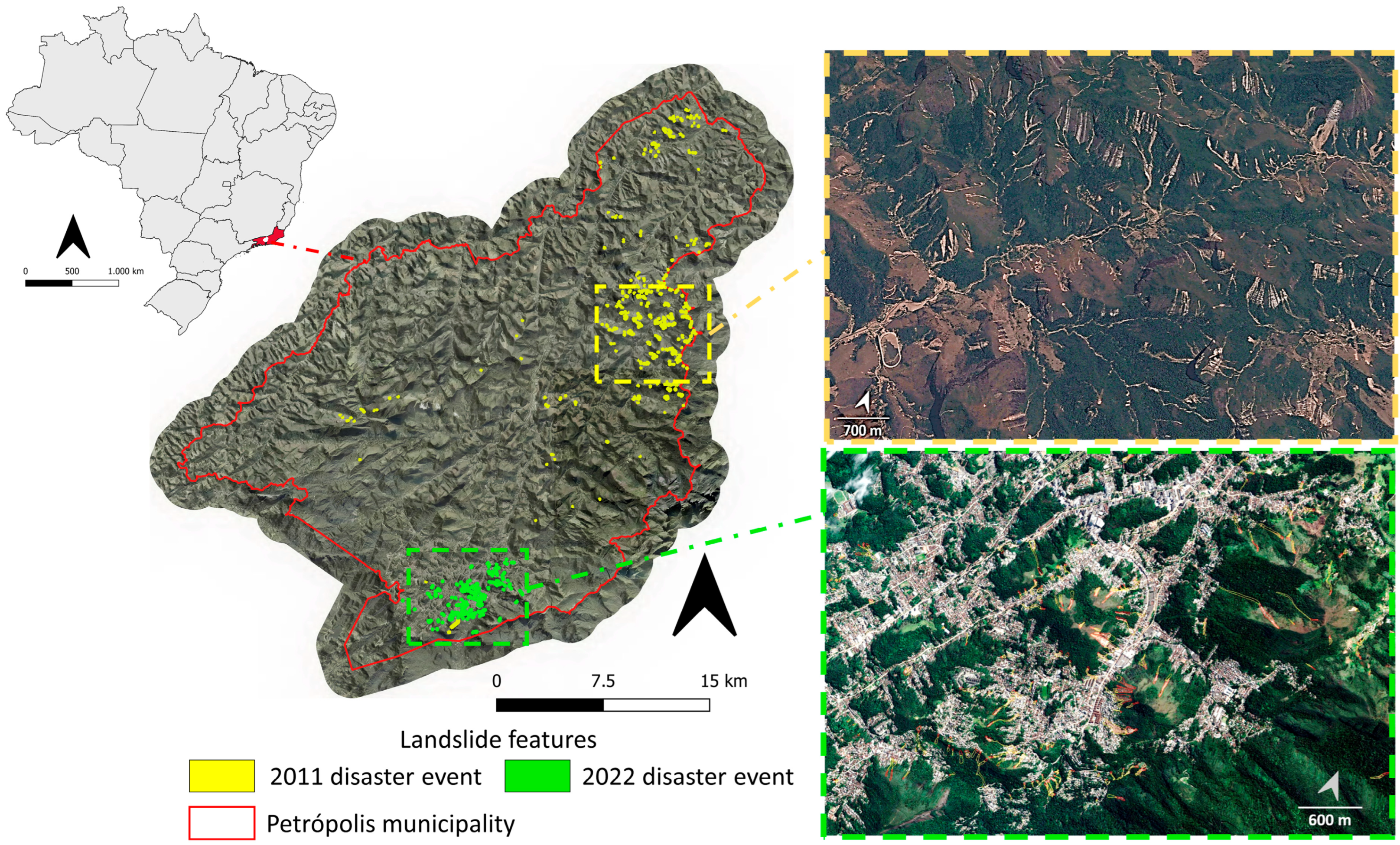
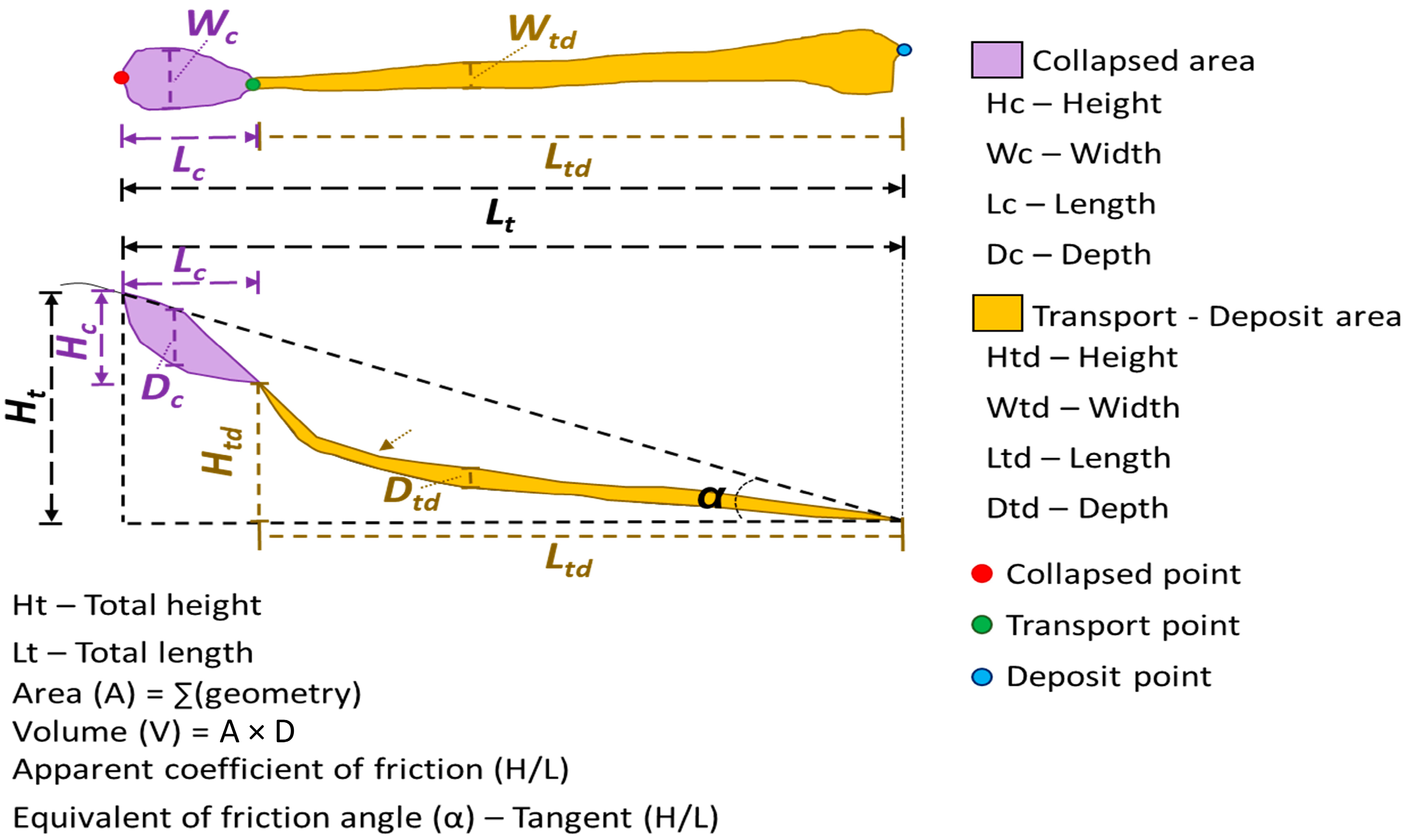
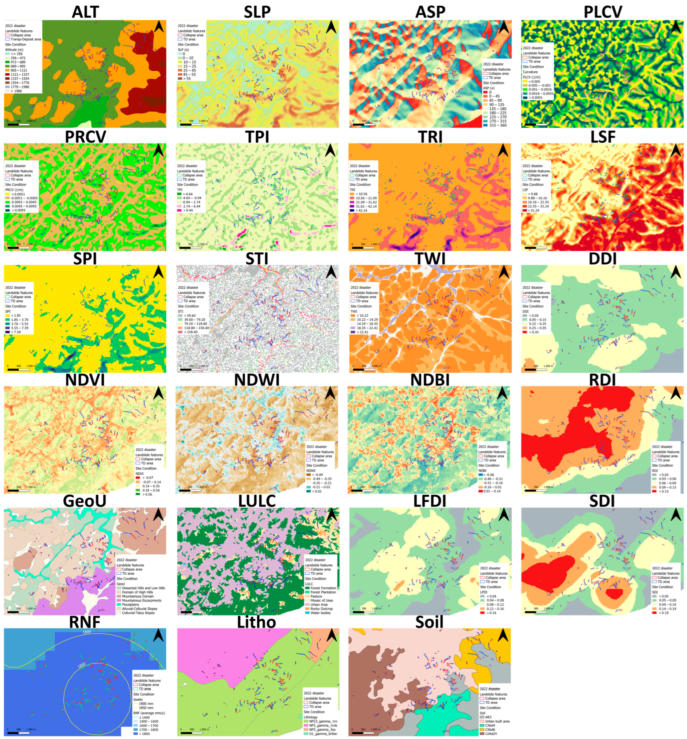
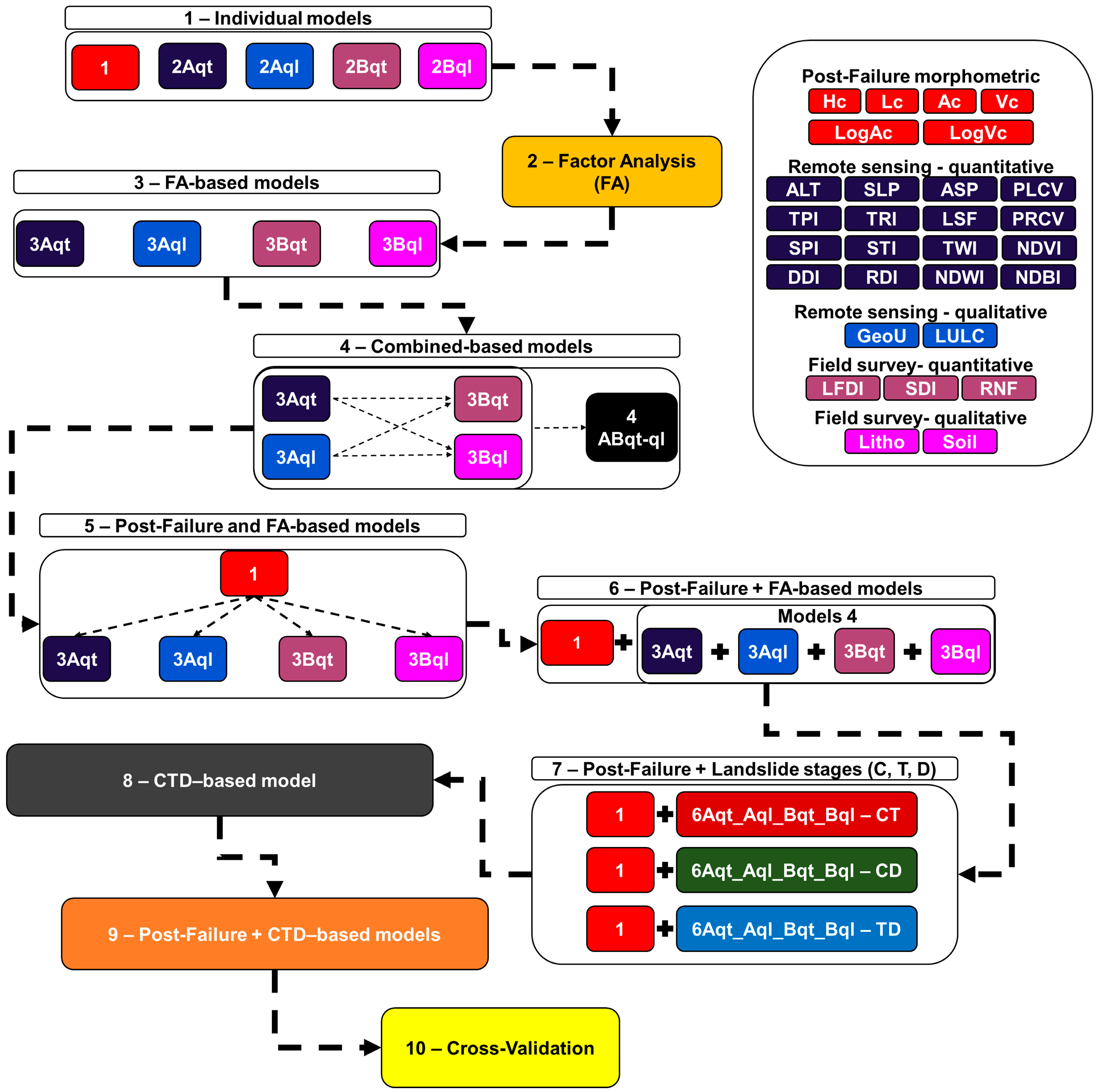

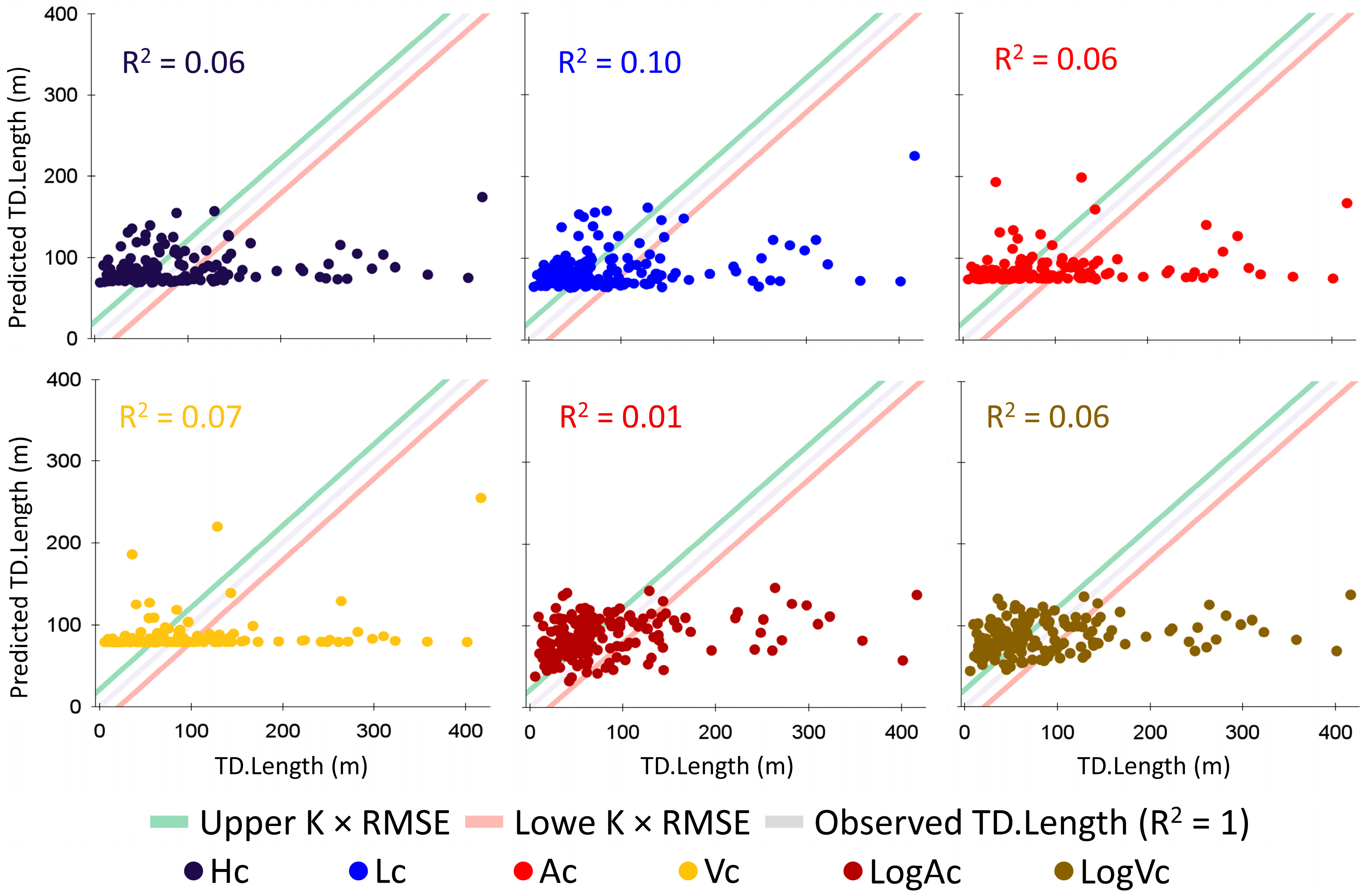
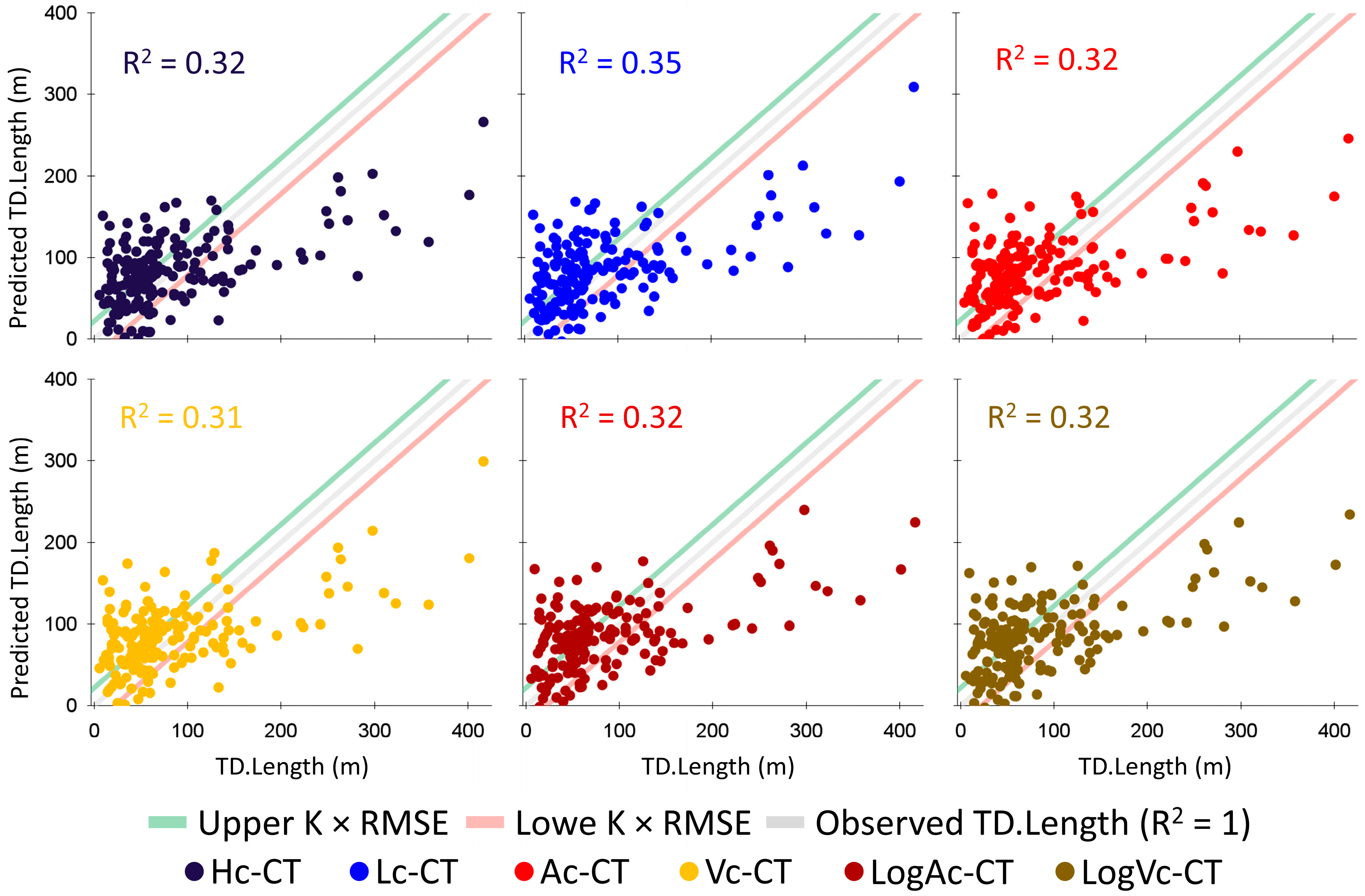
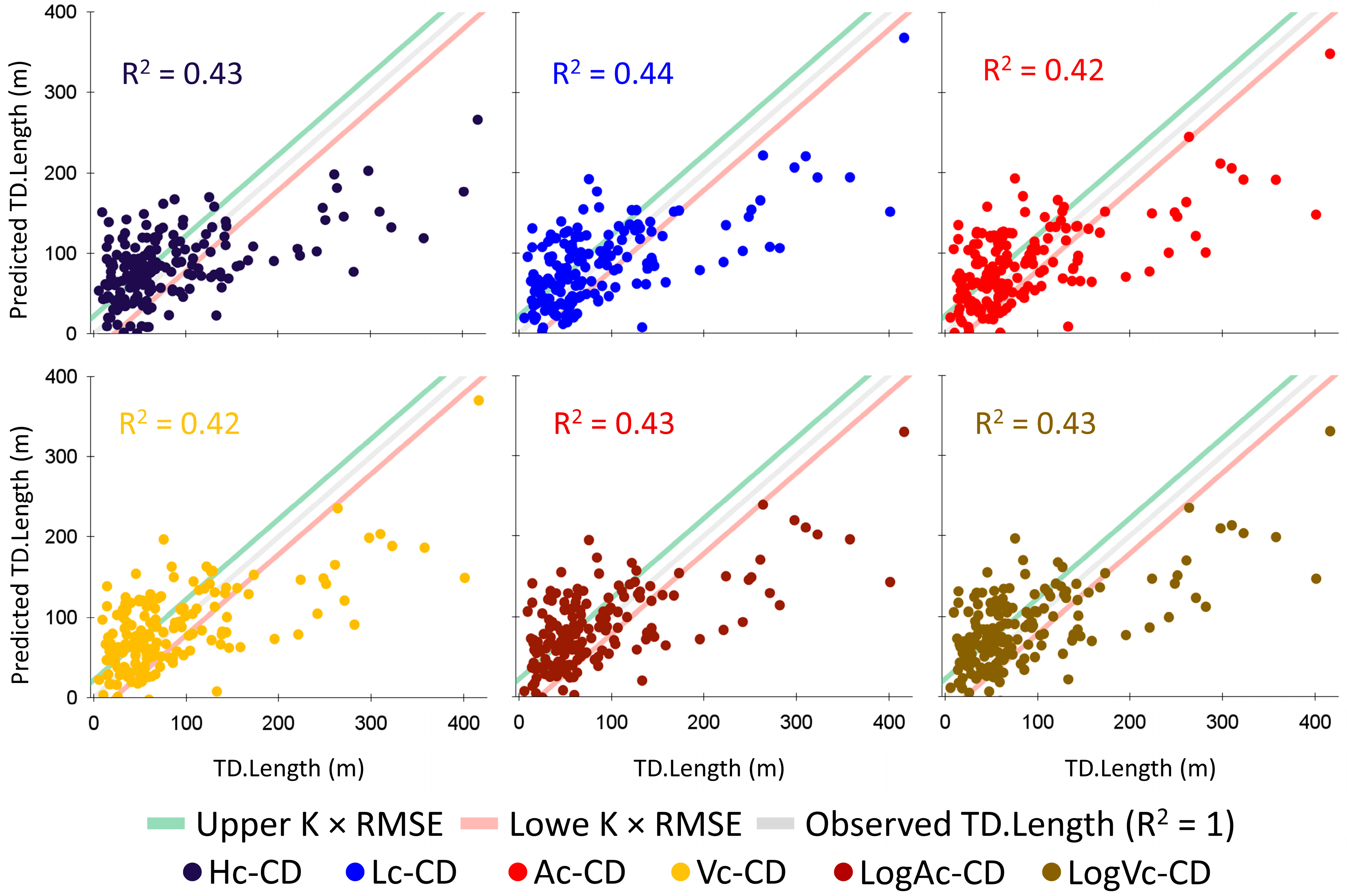
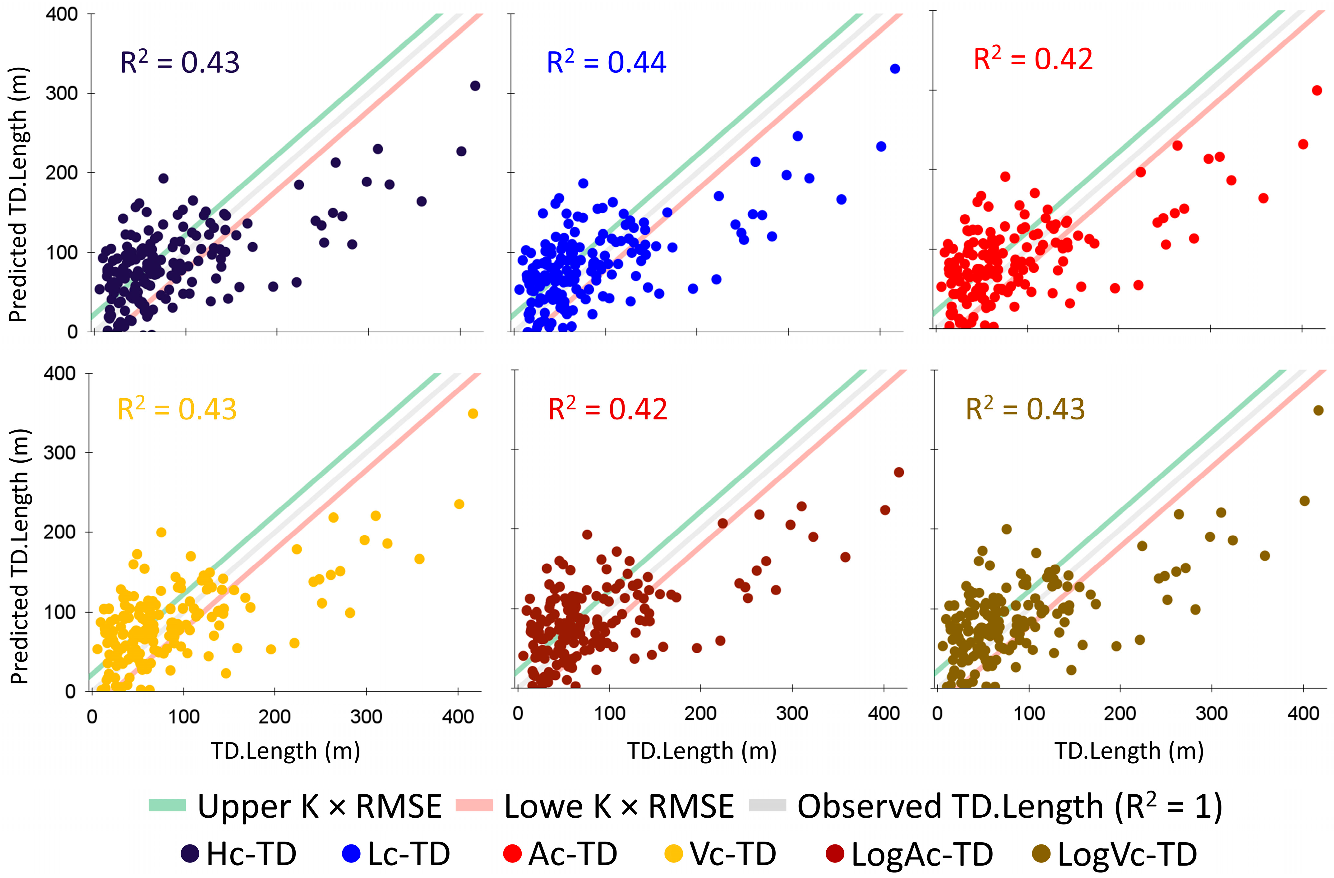
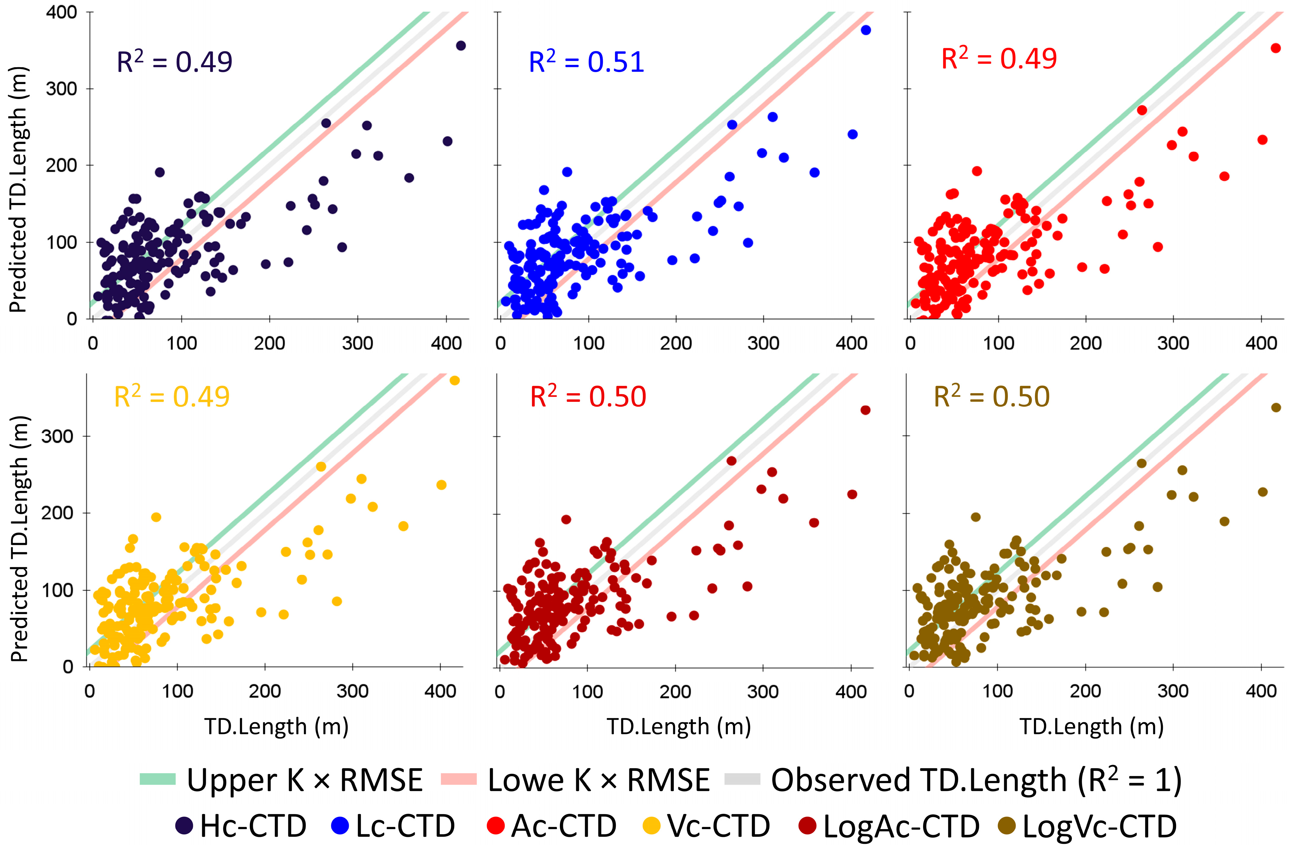
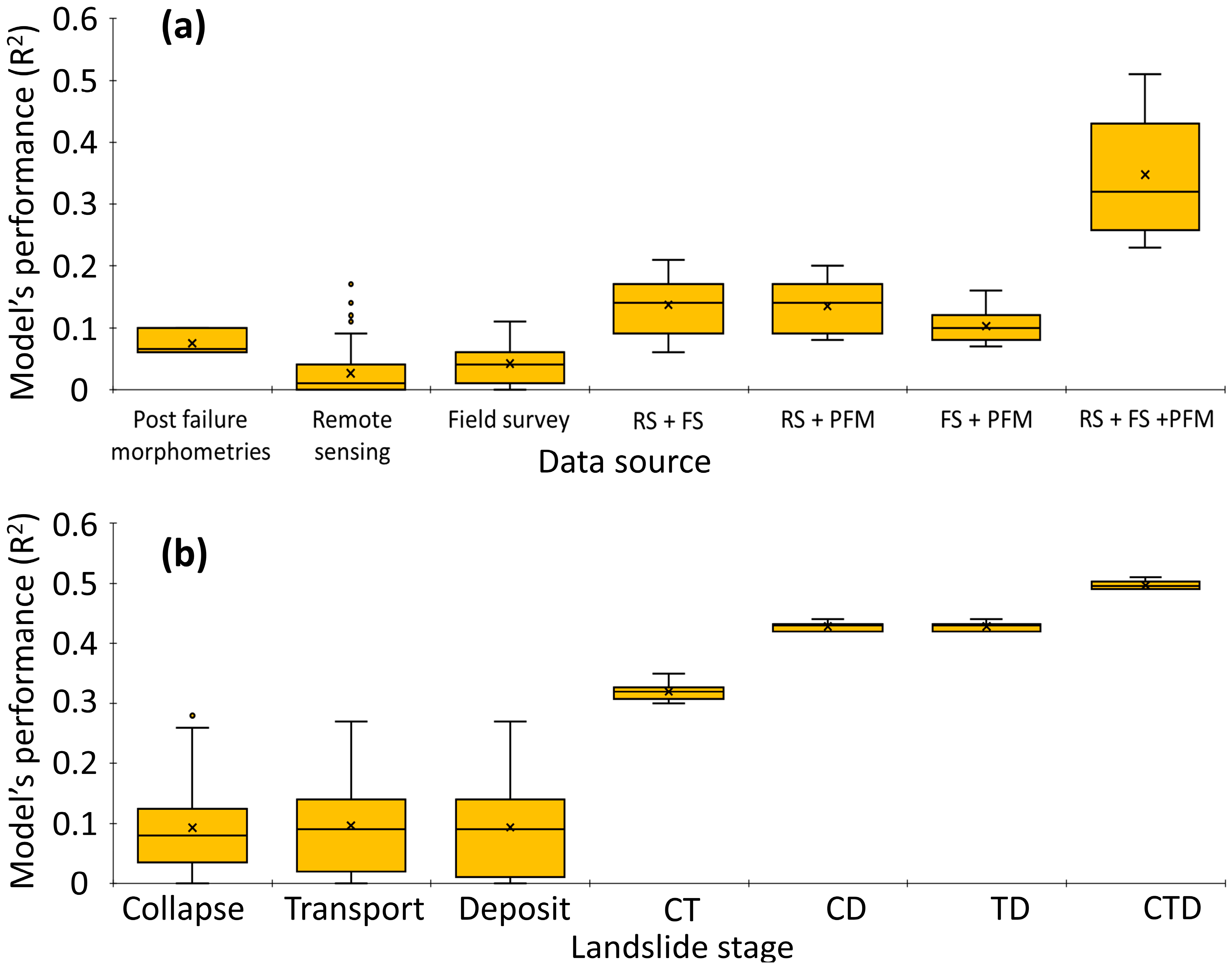
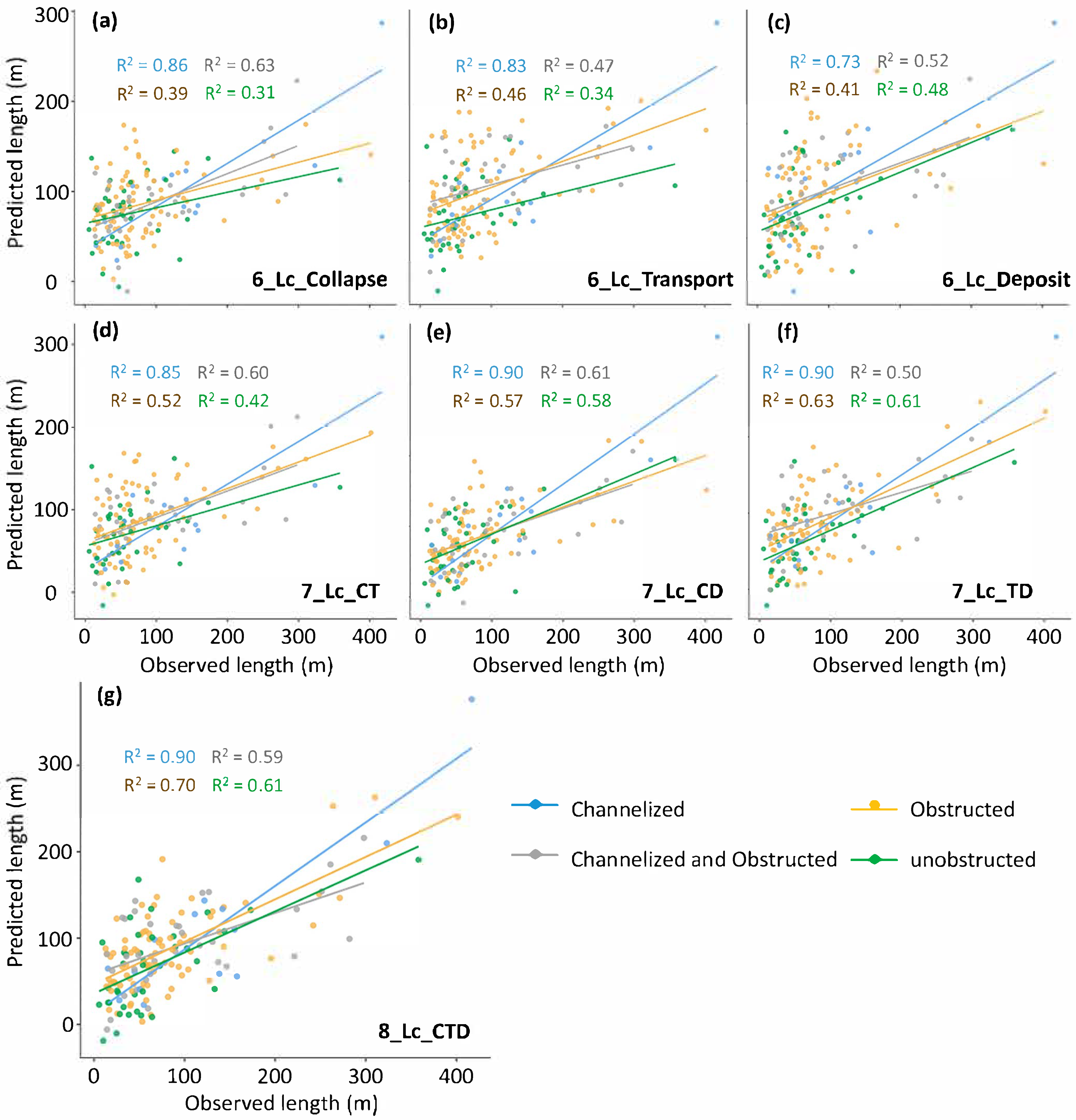
| Category | Type | Variable | Source |
|---|---|---|---|
| Remote Sensing (RS) | Quantitative (Qt) | Altitude (ALT) | DEM SRTM (30 × 30 m) |
| Slope angle (SLP) | |||
| Aspect (ASP) | |||
| Plan curvature (PLCV) | |||
| Profile curvature (PRCV) | |||
| Topographical Position Index (TPI) | |||
| Topographic roughness index (TRI) | |||
| Length-Slope Factor (LSF) | |||
| Stream Power Index (SPI) | |||
| Sediment Transport Index (STI) | |||
| Topographic Wetness Index (TWI) | |||
| Drainage density index (DDI) | |||
| Normalized Difference Water Index (NDWI) | Landsat 8 OLI (30 × 30 m) | ||
| Normalized Difference Vegetation Index (NDVI) | |||
| Normalized Difference Building Index (NDBI) | |||
| Road density index (RDI) | [84]—1:25,000 | ||
| Qualitative (Ql) | Geomorphological units (GeoU) | [58] | |
| Land Use Land Cover (LULC) | [55] | ||
| Field Survey (FS) | Quantitative (Qt) | Lineament—Fault density index (LFDI) | Geological maps |
| Structural density index (SDI) | 1:100,000 | ||
| Rainfall (RNF) | 1:50,000 | ||
| Qualitative (Ql) | Lithology type | Geological map (1:100,000) | |
| Soil type | Pedological map (1:100,000) |
| Qualitative | Code | Description |
|---|---|---|
| Lithology | NP23_gamma_1rn | Neoproterozoic diorites, tonalites, gabbros, and gneisses. |
| NP3_gamma_1rnb | Neoproterozoic gneisses and migmatites. | |
| NP3_gamma_1so | Neoproterozoic granites. | |
| O1_gamma_6nfan | Phanerozoic granites. | |
| NP2_gamma_3sor | Neoproterozoic orthogneisses. | |
| Soil | AR3 | Rock outcrop, associated with secondary cambisols and tertiary litholic neosols. |
| LVAd24 | Dystrophic Red-Yellow latosol, clayey or loamy. | |
| CXbd4 | Haplic cambisol Tb, dystrophic, medium or argillic; associated with a talic B horizon. | |
| CXbd6 | Haplic cambisol Tb, dystrophic, clayey or medium; associated with a talic B horizon. | |
| Urban area | Urban area | |
| Geomorphological unit | Alluvial-colluvial slopes | Gently inclined depositional surfaces (5–10°) composed of poorly sorted sandy-clayey to clayey-sandy colluvial materials, interdigitated with flat fluvial plain deposits. |
| Colluvial-talus slopes | Depositional slopes (5–10°) composed of very poorly sorted colluvial materials with sandy-clayey to clayey-sandy matrix and abundant blocks, interdigitated with gently inclined alluvial-colluvial ramp deposits. Typically located at the base of steep slopes and escarpments. | |
| Dissected hills and low hills | Convex-concave slopes and rounded hilltops with relief amplitude between 50 and 120 m and slopes of 5–20°. Moderate drainage density. | |
| Flood plains | Sub-horizontal surfaces (0–3°) located in valley bottoms, composed of well-sorted sandy, sandy-clayey, or clayey deposits. | |
| High hill domains | Convex-concave geometry with well-dissected terrain, rounded to pointed summits, relief amplitude of 80–250 m, slopes of 10–35°, and moderate to high drainage density. | |
| Mountainous domains | Straight to concave slopes with aligned ridge tops, pointed or slightly rounded, relief amplitude >300 m. High drainage density, with steep slopes (20–45°) and occasional sub-vertical rocky walls. | |
| Mountainous escarpments | Highly dissected, steep slopes (>300 m relief amplitude, 30–45° slope), with straight to concave profiles, rocky cliffs, and sharp or aligned ridge tops. High drainage density. | |
| Land Use and Land Cover | Forest formation | Vegetation types with a predominance of tree species with high-density continuous canopy. |
| Mosaic of uses | Farming areas where it was not possible to distinguish between pasture and agriculture. In Petropolis is often associated with the transition between informal settlements and areas that have been deforested. | |
| Pasture | Natural or planted, related to farming activity. | |
| Rock outcrop | Naturally exposed rocks in the terrestrial surface without soil cover, often with partial presence of rock vegetation and high slope. | |
| Urban area | Urban areas with a predominance of non-vegetated surfaces, including roads, highways and constructions. |
| Post-Failure Morphometric Variables | Transport-Deposit Length |
|---|---|
| Collapse height (Hc) | 0.24 |
| Collapse width (Wc) | 0.19 |
| Collapse length (Lc) | 0.22 |
| Collapse altitude (ALTc) | 0.13 |
| Collapse slope angle (SLPc) | 0.12 |
| Transport-Deposit height (Htd) | 0.32 |
| Transport-Deposited width (Wtd) | 0.26 |
| Transport altitude (ALTt) | 0.05 |
| Transport slope angle (SLPt) | 0.12 |
| Deposit altitude (ALTd) | −0.05 |
| Deposit slope angle (SLPd) | 0.02 |
| Total height (Ht) | 0.32 |
| Total length (Lt) | 0.89 |
| Total volume (Vt) | 0.62 |
| Variables | Collapsed | Transported | Deposited |
|---|---|---|---|
| ALT | 0.13 | 0.06 | −0.05 |
| SLP | 0.12 | 0.12 | 0.02 |
| ASP | 0.26 | 0.28 | 0.15 |
| PLCV | 0.18 | 0.13 | 0.11 |
| PRCV | 0.13 | 0.13 | 0.01 |
| TPI | 0.23 | 0.19 | 0.12 |
| TRI | 0.13 | 0.13 | 0.07 |
| SPI | 0.10 | 0.11 | 0.06 |
| LSF | 0.02 | 0.04 | −0.01 |
| STI | −0.02 | 0.03 | −0.01 |
| TWI | −0.18 | 0.13 | −0.08 |
| DDI | 0.01 | 0.01 | 0.05 |
| NDWI | 0.15 | 0.05 | 0.02 |
| LFDI | −0.14 | −0.14 | −0.18 |
| SDI | −0.19 | −0.18 | −0.18 |
| NDVI | −0.26 | −0.11 | −0.07 |
| RNF | 0.05 | 0.07 | 0.09 |
| RDI | 0.00 | 0.02 | 0.05 |
| NDBI | 0.23 | 0.04 | 0.05 |
| CTD_Based | 10-Fold Cross-Validation | ||
|---|---|---|---|
| Models | R2 | RMSE | MAE |
| CTD-based | 0.12 | 71.66 | 48.18 |
| Hc_CTD | 0.12 | 71.63 | 48.19 |
| LC_CTD | 0.15 | 70.33 | 47.58 |
| Ac_CTD | 0.10 | 72.56 | 48.48 |
| Vc1.0_CTD | 0.10 | 72.58 | 48.79 |
| LogAc_CTD | 0.11 | 71.82 | 48.06 |
| LogVc1.0_CTD | 0.12 | 71.56 | 47.76 |
Disclaimer/Publisher’s Note: The statements, opinions and data contained in all publications are solely those of the individual author(s) and contributor(s) and not of MDPI and/or the editor(s). MDPI and/or the editor(s) disclaim responsibility for any injury to people or property resulting from any ideas, methods, instructions or products referred to in the content. |
© 2025 by the authors. Licensee MDPI, Basel, Switzerland. This article is an open access article distributed under the terms and conditions of the Creative Commons Attribution (CC BY) license (https://creativecommons.org/licenses/by/4.0/).
Share and Cite
dos Santos, T.D.; Uchida, T. The Role of Collecting Data on Various Site Conditions Through Satellite Remote Sensing Technology and Field Surveys in Predicting the Landslide Travel Distance: A Case Study of the 2022 Petrópolis Disaster in Brazil. Remote Sens. 2025, 17, 3337. https://doi.org/10.3390/rs17193337
dos Santos TD, Uchida T. The Role of Collecting Data on Various Site Conditions Through Satellite Remote Sensing Technology and Field Surveys in Predicting the Landslide Travel Distance: A Case Study of the 2022 Petrópolis Disaster in Brazil. Remote Sensing. 2025; 17(19):3337. https://doi.org/10.3390/rs17193337
Chicago/Turabian Styledos Santos, Thiago Dutra, and Taro Uchida. 2025. "The Role of Collecting Data on Various Site Conditions Through Satellite Remote Sensing Technology and Field Surveys in Predicting the Landslide Travel Distance: A Case Study of the 2022 Petrópolis Disaster in Brazil" Remote Sensing 17, no. 19: 3337. https://doi.org/10.3390/rs17193337
APA Styledos Santos, T. D., & Uchida, T. (2025). The Role of Collecting Data on Various Site Conditions Through Satellite Remote Sensing Technology and Field Surveys in Predicting the Landslide Travel Distance: A Case Study of the 2022 Petrópolis Disaster in Brazil. Remote Sensing, 17(19), 3337. https://doi.org/10.3390/rs17193337


