Article

Cloud Mask Detection by Combining Active and Passive Remote Sensing Data

Hubei Key Laboratory of Regional Ecology and Environmental Change, School of Geography and Information Engineering, China University of Geosciences, Wuhan 430078, China
*
Author to whom correspondence should be addressed.
These authors contributed equally to this work.
Remote Sens. 2025, 17(19), 3315; https://doi.org/10.3390/rs17193315
Submission received: 16 August 2025 / Revised: 23 September 2025 / Accepted: 25 September 2025 / Published: 27 September 2025
(This article belongs to the Special Issue Remote Sensing in Clouds and Precipitation Physics)

Abstract

Highlights

Main Findings
  • A transfer learning-based model for cloud detection by combining CALIOP active remote sensing data and MODIS passive remote sensing data.
  • A consistency analysis of cloud mask detection across FY-4A/AGRI, FY-4B/AGRI and Himawari-8/9 AHI.
Implication of the Main Finding
  • Cross-validation of multi-source datasets shows that the cloud mask algorithm in this study is highly accurate and stable.
  • Results revealed that the cloud mask results of different satellite maintain high consistency, providing a robust foundation for the development of cloud datasets integrated.

Abstract

Clouds cover nearly two-thirds of Earth’s surface, making reliable cloud mask data essential for remote sensing applications and atmospheric research. This study develops a TrAdaBoost transfer learning framework that integrates active CALIOP and passive MODIS observations to enable unified, high-accuracy cloud detection across FY-4A/AGRI, FY-4B/AGRI, and Himawari-8/9 AHI sensors. The proposed TrAdaBoost Cloud Mask algorithm (TCM) achieves robust performance in dual validations with CALIPSO VFM and MOD35/MYD35, attaining a hit rate (HR) above 0.85 and a cloudy probability of detection ( P O D c l d ) exceeding 0.89. Relative to official products, TCM consistently delivers higher accuracy, with the most pronounced gains on FY-4A/AGRI. SHAP interpretability analysis highlights that 0.47 μm albedo, 10.8/10.4 μm and 12.0/12.4 μm brightness temperatures and geometric factors such as solar zenith angles (SZA) and satellite zenith angles (VZA) are key contributors influencing cloud detection. Multidimensional consistency assessments further indicate strong inter-sensor agreement under diverse SZA and land cover conditions, underscoring the stability and generalizability of TCM. These results provide a robust foundation for the advancement of multi-source satellite cloud mask algorithms and the development of cloud data products integrated.

1. Introduction

Clouds are an essential component of Earth’s atmospheric system, with a global coverage of approximately 70% [1]. Clouds strongly affect atmospheric processes and climate monitoring, making reliable cloud identification a key task in Earth observation [2,3]. In remote sensing applications, cloud cover can obscure surface reflectance signals, resulting in image distortion and affecting the extraction and analysis of surface parameter retrievals [4,5]. Therefore, accurate cloud detection has become a fundamental and essential step in remote sensing data preprocessing. As the core product of cloud detection, cloud mask is crucial for both remote sensing analysis and atmospheric studies. High-quality cloud mask datasets provide essential support for climate research, ecological monitoring, and satellite-based environmental applications [6,7].
Currently, cloud mask data are primarily obtained via two approaches: direct and indirect observations. The former includes ground-based observations such as ceilometers and active remote sensing technologies such as spaceborne lidars, while the latter relies on passive optical sensors for wide-scale observations. Among the direct methods, ground observation stations are fewer and have higher requirements for installation environment and maintenance. Space-borne active remote sensing technologies are less affected by weather conditions and can provide high-precision, vertically detailed cloud information. In particular, the Cloud-Aerosol Lidar with Orthogonal Polarization (CALIOP) onboard the Cloud-Aerosol Lidar and Infrared Pathfinder Satellite Observations (CALIPSO) satellite provides a Vertical Feature Mask (VFM) dataset, which offers high vertical resolution and strong, highly reliable cloud detection capabilities [8,9]. However, active remote sensing observes vertically in a narrow swath and has limited spatial coverage. In addition, ground-based observation data are sparsely distributed and insufficient to support large-scale research. In contrast, passive satellite sensors, such as the Moderate Resolution Imaging Spectroradiometer (MODIS), with larger coverage, stable operation, and richer information in a single observation, can provide global-scale data within a short time frame. It can effectively compensate for the limitations of active remote sensing and is an important data source for detecting clouds effectively. Although MODIS products are widely recognized for their global coverage and long-term data accumulation, they have longer revisit periods and lower temporal resolution. Geostationary satellite sensors, such as the Advanced Geosynchronous Radiation Imager (AGRI) and the Advanced Himawari Imager (AHI), offer higher temporal resolution observations in specific regions, providing more detailed and frequent remote sensing information.
In light of the characteristics of different remote sensing data sources, various cloud detection algorithms have been proposed, including traditional spectral threshold algorithms [10] and emerging machine learning and deep learning algorithms [10,11,12,13]. Threshold algorithms mainly utilize the high-reflectance and low-brightness temperature characteristics of clouds to apply discriminative thresholds based on the spectral characteristics of different sensors and bands. These algorithms offer simplicity and stable performance, but tend to exhibit larger errors in high-albedo backgrounds or when detect thin clouds [14]. With the development of computer hardware and artificial intelligence, machine learning algorithms have been increasingly applied. Compared to threshold algorithms, machine learning algorithms require fewer assumptions and prior knowledge, making them more efficient and flexible. Some studies have combined threshold algorithms with machine learning to improve cloud detection accuracy under complex surface conditions [15,16].
Although recent cloud masking algorithms, such as those developed by Shang et al. [15] for Himawari-8 and Choi et al. [17] for Geo-Kompsat-2A, have demonstrated improved performance over official products, most existing studies still focus on individual satellite sensors. In reality, differences in observation principles, spectral responses, temporal resolution, and spatial coverage across various sensors will lead to inconsistencies and uncertainties in cloud detection results. These discrepancies limit the cross-platform applicability of cloud products and pose challenges for multi-source combination and consistency assessment. Integrating cloud masks from different satellites, especially geostationary platforms, can enhance detection reliability and support multi-scale applications in meteorological forecasting and ecological monitoring [18,19]. However, the cloud mask quality across different products exhibits considerable uncertainty. Some studies have shown that changes in ice particle models across MODIS product versions can result in substantial differences in cloud masks [20,21]. Even datasets from the same sensor processed using different algorithms show inconsistencies, let alone those from different sensors. Lai et al. [22] reported that the difference in cloud mask pixel proportions between AGRI and MODIS was less than 2%, while that between AHI and MODIS exceeded 10%. These differences arise from sensor performance, spectral response functions, and retrieval algorithms. However, current research on cloud mask discrepancies primarily focuses on comparing products from different algorithms [22,23], with limited investigation and comparisons into the differences of cloud detection results across satellite platforms. Although Wang et al. [24] developed a unified algorithm to compare the cloud mask performance of FY-4A and Himawari-8, the analysis was limited to accuracy assessment, without further explore the consistency characteristics and influencing factors of multi-source cloud products. A systematic evaluation of the consistency among different cloud mask products is essential for improving the efficiency of multisensor data fusion and remote sensing collaborative applications.
Most of the above algorithms mainly use MODIS or CALIOP cloud mask products as reference datasets [25,26,27,28]. However, both MODIS and CALIOP have limitations. MODIS sensors primarily rely on visible and infrared channels for feature identification, which limits their sensitivity to cloud structure and vertical distribution under complex surface conditions [9,29]. Meanwhile, CALIOP has a limited observational swath which restricts its applicability in large-scale validation.
In this context, transfer learning has emerged as a promising approach for combining active and passive remote sensing data, owing to its cross-domain adaptability [30,31]. Transfer learning is a technique that utilizes knowledge from source domain to improve learning performance in target domain, particularly in scenarios where data distributions differ but remain related [32]. Traditional machine learning algorithms often rely on the assumption that training and test data share the same distribution. However, in remote sensing applications, this assumption may not hold because of differences in sensor characteristics and observational conditions. Transfer learning can alleviate the performance degradation caused by these discrepancies and improve the generalization ability of the model [33].
Common transfer learning methods include fine-tuning [34], domain adaptation [35,36], and instance-based transfer learning [37]. For instance, Li et al. [34] applied fine-tuning transfer learning to retrieve cloud properties by combining Himawari-8 and MODIS data, achieving better accuracy than official Himawari-8 products. Mateo-Garcia et al. [36] proposed the adversarial domain adaptation framework, effectively reduced the distribution gap between different sensors and improved cloud detection accuracy. These studies confirmed the feasibility and advantages of applying transfer learning and combining multiple sensor data sources. However, both fine-tuning and domain adaptation have limitations, including the risk of overfitting and negative transfer, as well as high computational costs, and reliance on extensive hyperparameter tuning. In contrast, instance-based transfer learning approaches such as TrAdaBoost provide a lightweight and efficient solution. For example, He et al. [37] proposed a multiclass TrAdaBoost algorithm for mobile LiDAR data classification, demonstrating that the method can effectively leverage source data while maintaining robustness when target-domain samples are scarce. This suggests that TrAdaBoost has strong potential for multisensor cloud mask detection tasks with limited labeled data.
Therefore, to address the limitations of single-sensor studies and the constraints of MODIS and CALIOP data, this study proposes a cloud mask framework based on the TrAdaBoost transfer learning algorithm for the first time. The framework leverages the advantages of MODIS and CALIOP to enable unified modeling and high-accuracy cloud detection across multiple geostationary satellite sensors. Furthermore, by incorporating a systematic analysis under varying observation angles and diverse land cover types, the study provides insights into the consistency of cloud mask detection across different satellite platforms, offering both methodological support and theoretical foundation for the integration of multi-source satellite cloud products. The study focuses on East Asia, a region characterized by active cloud–aerosol interactions, and involves four mainstream geostationary sensors: FY-4A/AGRI, FY-4B/AGRI, and Himawari-8/9 AHI. The study covers the period from July 2022 to June 2023. To minimize external interference, a consistent cloud mask algorithm is applied under a unified spatiotemporal framework. The algorithm is trained and validated using CALIPSO VFM and MOD35/MYD35 cloud mask datasets, and the consistency in cloud detection performance across these sensors are quantitatively assessed from multiple dimensions.

2. Data and Study Area

2.1. Geostationary Satellite Data

Geostationary orbit satellites are located over the equator at an altitude of about 36,000 km, and their observations cover about one third of the Earth’s surface, providing continuous observation data. In this study, full disk level data from FY-4A/AGRI, FY-4B/AGRI and H-8/AHI (H-9/AHI) geostationary satellite sensors, are used to detect cloud masks.
The Fengyun-4 meteorological satellite is a new generation of Chinese geostationary meteorological satellites, containing FY-4A and FY-4B, with the sub-satellite point of the two satellites changing with the change of the operation. During the study period, the sub-satellite points of FY-4A and FY-4B were 105°E and 133°E, respectively. The Advanced Geostationary Radiation Imager (AGRI) deployed on FY-4A and FY-4B provides level-1 data and other level-2 products such as atmospheric, terrestrial, oceanic, and radiation data. However, the two satellites are not fully synchronized in operation. Relative to FY-4A/AGRI, FY-4B/AGRI significantly improves its observation performance, observation bands, and data transmission capability, not only increasing the water vapor detection channel, but also further improving the observation temporal and spatial resolution. In addition, the geolocation information observed by AGRI is provided by GEO data files, including solar zenith angle, solar azimuth angle, satellite zenith angle and satellite azimuth angle.
Himawari-8/9 is a new generation of Japanese geostationary meteorological satellites [38], which has an Advanced Himawari Imager (AHI) similar to the Advanced Baseline Imager (ABI) sensor of the GOES series of satellites. The operation of Himawari-8 (H-8) started in July 2015, and Himawari-9 (H-9) in 2017 March, and H-9 began backup operation and officially succeeded H-8 as the main meteorological satellite of JMA on 13 December 2022. H-8/AHI and H-9/AHI have the same hardware and technology, with basically the same band configuration, and have the capability of synchronized observation in the time frame of this study, which ensures the reliability and continuity of data for both. AHI has 16 observational bands characterized by high temporal resolution and multi-spectral observation, and also provides level-1 data and level-2 products such as clouds and radiation. Among them, the level-1 data files contain geolocation information.
Detailed parameters of the geostationary satellite sensors in this study are shown in Table 1. In order to eliminate the differences in the band settings of different satellite sensors, the study only used channels that existed in these sensors at the same time, as shown in the first column in Table 2.
In this study, level-1 data from AGRI-A, AGRI-B, and AHI were subjected to projection transformation and radiometric calibration. They were then matched with CALIOP data within a 5 min time window; the detailed matching procedure is described in Section 2.2. The geostationary satellite data used include the bands highlighted in Table 2, as well as solar zenith angle (SZA), satellite zenith angle (VZA), and relative azimuthal angle (RAA), which is defined as the absolute value of the difference between the solar azimuth and the satellite azimuth.
The full-disk observation coverage of AGRI-A, AGRI-B, and AHI, as well as the study area of this research, are shown in Figure 1. The East Asian region was selected as the study area, focusing on Chinese land, with a longitude range of 80°E–136°E and a latitude range of 17°N–54°N.

2.2. CALIPSO VFM

The CALIPSO satellite, jointly developed by NASA and the French Space Agency, carries visible and near-infrared polarimetric lidar sensors (CALIOP) capable of providing detailed information on the distribution and characteristics of global aerosols and clouds in the vertical direction [39]. CALIPSO withdrew from the A-Train formation after 2018, and the time lag between its observations and MODIS sensors increased significantly.
The CALIPSO Level 2 Vertical Mask Feature (VFM) product provides vertically distributed data on clouds, aerosols, ground, and other atmospheric features that can be effectively applied to cloud detection. This study used the CALIPSO VFM dataset as a benchmark to validate the cloud mask algorithm, and adopted the cloud mask processing of Wang et al. [40] for the CALIPSO VFM dataset by first sampling the CALIPSO VFM data uniformly in the vertical direction with a horizontal resolution up to 333 m, and then matching it with the FY-4A, FY-4B, and the AHI to statistically 5 min time difference, the number of CALIPSO VFM observations in the 4000 m (or 5000 m) spatial range, and the cloud probability. When the cloud probability is 1, clouds are considered to be detected at that range. For FY-4A and FY-4B, only data with more than 12 CALIPSO VFM observations at the 4 km spatial range are retained. For AHI, data with more than 15 CALIPSO VFM observations in the 5 km spatial range were considered valid.

2.3. MOD35/MYD35

MODIS sensors were launched onboard the Terra and Aqua satellites in 1999 and 2002, respectively, and provide a variety of products covering the atmosphere, land, and ocean. Among them, the cloud mask dataset for the Terra satellite (MOD35) and the cloud mask dataset for the Aqua satellite (MYD35) provide 1 km spatial resolution cloud mask data. MOD35 and MYD35 datasets algorithms are based on MODIS visible and infrared bands, using a series of threshold tests to calculate the clear-sky confidence level for each pixel, and ultimately classifying the observed pixels into four categories: clear, probably clear, probably cloudy, and cloudy based on three thresholds: 0.99, 0.95, and 0.66 [41]. After the continuous updating and enhancement of MODIS cloud retrieval algorithm, the product has good usability [42].
Compared with active LiDAR, passive optical sensors have a larger coverage of a single observation, rich observation information, and can acquire global data in a short period. Considering the limitation of CALIPSO VFM, we added MOD35 and MYD35 data to jointly verify the cloud mask algorithm performance.

2.4. Land Cover Type Data

The MODIS land cover type product (MCD12Q1) provides annual 500 m spatial resolution global land cover datasets from 2001 to present, which contain five traditional classification schemes [43]. In this study, we used the land cover type data based on the International Geosphere-Biosphere Programme (IGBP), and referred to the reclassification idea of Wang et al. [13] for IGBP, and regrouped the results of the 17 land cover types of IGBP into seven categories of forests, shrublands/grasslands, croplands, urban, barren, snow/ice, and wetlands/waters. The results of the land cover types of IGBP and the reclassification are demonstrated in Table 3 and Figure 1.

3. Methods

3.1. Random Forest

Random Forest (RF) is a nesting-based method developed by Breiman in 2001 [44], which uses the ensemble machine learning technique of regression trees. Random forest introduces randomness in the process of tree construction; for example, the tree can be constructed by randomizing the feature set and dataset. The specific steps of RF algorithm are as follows:
  • Bootstrap sampling: From a total of N training samples, n bootstrap samples are drawn with replacement to form n training sets. The remaining unsampled data in each set, called out-of-bag data, are used to estimate prediction error.
  • Feature selection: At each node of a decision tree, randomly select m features (m < M, where M is the total number of input variables), and determine the optimal split based on these m features. Each tree is grown to its maximum depth without pruning.
  • Prediction aggregation: A random forest is formed from the generated multiple decision trees, and the random forest is used to do regression analysis, and the average of the output results of each decision tree is used as the prediction value, as shown in the following equation:
    Y x i = 1 n 1 n T n x i  
    where T n is each decision tree and n is the number of decision trees.

3.2. TrAdaBoost

TrAdaBoost is an instance-based transfer learning algorithm designed to improve predictive performance in a target domain by leveraging labeled data from a related source domain [45]. It is derived from Adaptive Boosting (AdaBoost) proposed by Freund and Schapire [46], an ensemble learning method that iteratively combines multiple weak classifiers, increasing the weights of misclassified samples and aggregating predictions through weighted voting to enhance model accuracy.
While AdaBoost assumes that training and test data are drawn from the same distribution, its performance can degrade under distribution shifts between source and target domains. TrAdaBoost addresses this limitation by introducing a dynamic weight adjustment mechanism: during each iteration, the weights of misclassified source-domain samples are gradually decreased, whereas the influence of target-domain samples is progressively increased. This strategy mitigates negative transfer and enables effective utilization of abundant source-domain data even when target-domain labeled samples are scarce. As a result, TrAdaBoost is particularly suitable for multi-source data integration and heterogeneous domain learning tasks, achieving high predictive accuracy with limited target-domain data.
Considering that the MODIS and CALIOP data used in this study have different distributions, in order to fully combine the advantages of MODIS passive optical data and CALIOP active LIDAR data, the study adopts the TrAdaBoost algorithm where MODIS data are used as the source domain and CALIOP data as the target domain.
The details of the TrAdaBoost algorithm are described as follows:
  • Initialize the weights in the source domain and the target domain:
    w i 1 = 1 / n ,           i = 1 ,   , n   ( s o u r c e   d o m a i n ) 1 / m ,         i = n + 1 ,   , n + m   ( t a r g e t   d o m a i n )
    where n is the number of samples in the source domain, m is the number of samples in the target domain, and w is the weight in the source domain and the target domain. These are unnormalized initial weights, and the sum of the weights within the source and target domains is 1.
  • Normalize weights of all samples and call a learner (basic machine learning algorithms):
    P t = w t i = 1 n + m w i t , t = 1 , , N
    where P t is the normalized weight of the sample in the source domain and target domain, N is the number of iterations, t is the iteration index, and w i t is the unnormalized weight of sample i in round t.
  • Calculate the error rate ( ϵ t ) of h t in the target domain:
    ϵ t = i = n + 1 n + m w i t · h t x i c x i i = n + 1 n + m w i t
    where h t is the classifier learned in the step. 2, x is an input variable, h t x i is the prediction of the weak classifier (or base learner) on sample x in the t round, and c x i is the actual label of x in the target domain. Note that ϵ t must be less than 0.5.
  • Calculate the weight adjustment rate β in the source domain and the weight adjustment rate β t in the target domain:
    β = 1 1 + 2 ln n / N
    β t = ϵ t / 1 ϵ t
    where β is constant during each iteration.
  • Update the weights of all samples:
    w i t + 1 = w i t   β h t x i c x i ,             1 i n   ( s o u r c e   d o m a i n ) w i t   β t h t x i c x i ,         n + 1 i m   ( t a r g e t   d o m a i n )
    where w i t + 1 is the unnormalized weight of sample i in round t+1.
  • Output the hypothesis:
    h f x = 1 ,     t = N / 2 N β t h t x   t = N / 2 N β t 1 / 2 0 ,     otherwise
    where h f x is the decision function used to predict the label of sample x.

3.3. Constructing the Cloud Mask Model

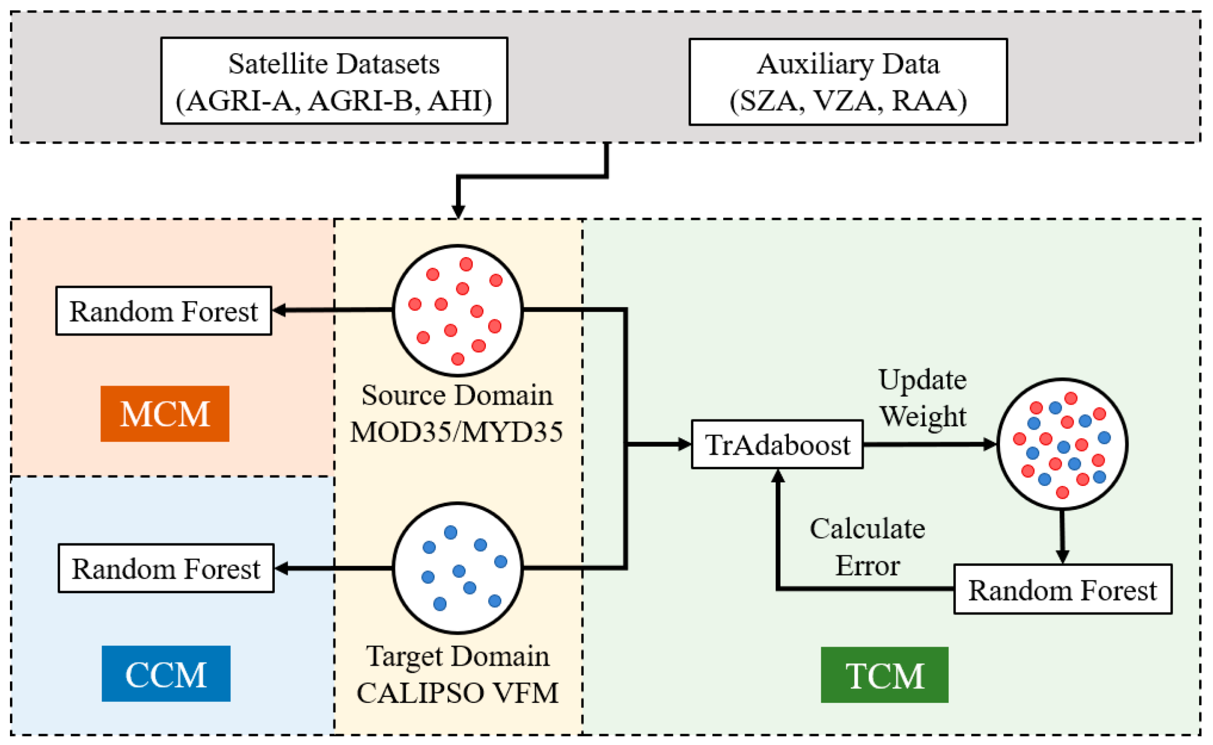
In this study, a TrAdaBoost transfer learning cloud mask algorithm is proposed, using RF as the base learner, MOD35/MYD35 data as the source domain and CALIPSO VFM data as the target domain. The method optimizes the model adaptation on the target domain (CALIOP) while retaining the advantage of the information in the source domain (MODIS) through the dynamic weight adjustment mechanism of TrAdaBoost. This mechanism ensures the model adapts effectively to the high-precision cloud features in CALIOP datasets while still benefiting from the vast information contained in MODIS datasets, so as to effectively improve the cloud mask detection accuracy.
The TrAdaBoost cloud mask algorithm is referred to as the “TCM” algorithm in the following. For comprehensive validation, two benchmark models were also constructed: MCM (MODIS-based Cloud Mask): An RF model trained exclusively with MODIS/MYD35 data; CCM (CALIOP-based Cloud Mask): An RF model trained exclusively with CALIPSO VFM data.
We matched the AGRI-A, AGRI-B, and AHI bands to MOD35/MYD35 and CALIPSO VFM cloud mask pixels. For MOD35/MYD35, “clear” and “probably clear” pixels are redefined as “clear”, and “cloudy” and “probably cloudy” pixels are redefined as “cloudy”; for CALIPSO VFM, a pixel is considered cloudy when it has a cloudy probability of 1 in the spatial resolution of the corresponding sensor (see Section 2.2).
Model inputs consist of the selected spectral bands listed in Table 2, together with geometric features including solar zenith angle (SZA), satellite zenith angle (VZA), and relative azimuth angle (RAA). The corresponding labels are derived from two sources: MOD35/MYD35 cloud mask data, serving as the source domain, and CALIPSO VFM cloud mask data, serving as the target domain. Crucially, CALIPSO VFM data is not merely for validation; it is directly integrated into the training process. Due to the huge amount of MOD35/MYD35 data, we extracted only 1% for model training and testing after disrupting the matched data. The final number of matches between AGRI-A, AGRI-B, and AHI with MOD35/MYD35 are 219,011,756, 218,914,853, and 143,243,702, and the number of matches with CALIPSO VFM are 11287, 11287, and 8139. The dataset is divided into two parts; 80% is used for training, and 20% is used for testing.
The frameworks of TCM, MCM, and CCM algorithms are shown in Figure 2.

3.4. Validation Metrics

Four metrics were used to validate the cloud mask detection model, including the probability of detection (POD), the false alarm ratio (FAR), the hit rate (HR), and the Kuiper’s skill score (KSS).
POD evaluates the model’s ability to correctly identify target pixels, where a value close to 1 is desirable. FAR quantifies the proportion of pixels that are falsely classified, and thus a lower value is preferred. HR measures the overall accuracy of classification, and a higher value indicates better agreement between predictions and observations. KSS considers both hit and false alarm rates and provides a balanced assessment of model skill; higher KSS values indicate stronger discriminative capability. All these metrics range from 0 to 1, with values closer to 1 (except for FAR) representing better model performance.
The definitions are as follows:
P O D c l d = a a + b
P O D c l r = d c + d
F A R c l d = c a + c
F A R c l r = b b + d
H R = a + d a + b + c + d
K S S = a d + b c a + b c + d
where c l d represents cloudy; c l r represents clear; a and d represents the number of pixels classified as cloudy and clear by both the benchmark and the model; b represent the number of pixels classified as cloudy by the benchmark but clear by the model; and c represent the number of pixels classified as clear by the benchmark but cloudy by the model. Table 4 provides references for these parameters.

3.5. SHAP Interpretability Analysis

To gain a deeper understanding of the cloud mask detection model and quantify the contribution of each input feature to the cloud mask predictions, we adopt SHapley Additive exPlanations (SHAP) analysis. This analysis helps identify the most influential features and validate the physical plausibility of the model, ensures that the model relies on meaningful features rather than spurious correlations.
SHAP is a game theory-based model interpretability method for quantifying the contribution of each input feature to the model prediction results [47]. The method is theoretically based on Shapley values and accurately evaluates the importance of each feature in the prediction process by calculating the marginal contribution over all possible subsets of features. SHAP not only provides a uniform and consistent feature importance metric, but also visualizes the positive or negative impact of features on the prediction results. It is widely used to improve the transparency and credibility of machine learning models, especially for the interpretation and analysis of nonlinear and complex models.
Shapley value is originally used in game theory to measure the fair contribution of the participants to the total return, and in model interpretation, it represents the contribution of each input feature to the predicted value of the model. The predicted value is given by the following equation:
f x = θ 0 + i = 1 M θ i
where f x is the predicted value of the model for sample x , θ 0 is a constant value (usually the average predicted value of all samples in the training set), θ i is the Shapley value of feature i , and M is the number of features.

4. Results

4.1. Cloud Mask Algorithm Validation

Table 5 and Table 6 present the performance evaluation results of the TCM cloud mask algorithm on AGRI-A, AGRI-B, and AHI, under the validation of CALIOP and MODIS data, respectively. A lower FAR (closer to 0) and higher values of the other metrics (closer to 1) indicate better classification performance. In general, the TCM algorithm shows strong cloud detection ability for all sensors. In both validation results, the KSS is more than 0.68, the HR is higher than 0.85, and the P O D c l d is more than 0.89, reflecting that the algorithm has better stability and recognition accuracy. Under the CALIOP validation, the HR and P O D c l d are more outstanding, both exceeding 0.91, indicating that the TCM algorithm has stronger adaptability when compared with the high-precision vertical observation data of LIDAR, and further verifying the effectiveness and applicability of the TrAdaBoost in target domain modeling. In particular, it is worth noting that the AHI sensor has the best performance in CALIOP validation, which not only achieves the highest values of P O D c l d , HR, and KSS, but also has the lowest value of F A R c l d , which reflects the strong cloud identification ability; the AGRI-A sensor has the second highest comprehensive performance, and the performance is also more robust. In MODIS validation, the results show a different trend: AGRI-A has the best performance, followed by AGRI-B, and AHI is relatively weak. This difference may be related to the observation methods and sensitivities of the different validation data sources, indicating that the sensor characteristics have a significant impact on the evaluation of the cloud mask algorithm under different reference data.
To compare the performance of the TCM, MCM, and CCM algorithms in multisensor cloud mask detection, Figure 3 and Figure 4 show the comprehensive performance of the three types of cloud mask algorithms validated based on CALIOP and MODIS data on three stationary orbit sensors, namely AGRI-A, AGRI-B, and AHI, respectively.
As expected, the CCM has the highest HR and KSS values on all sensors in the CALIOP validation. In contrast, the MCM algorithm, which is trained entirely based on the MODIS data, has a poor overall performance under the CALIOP evaluation, showing difficulty in generalizing the information from the source domain to the target domain. On the other hand, the HR and KSS values of the TCM algorithm are very close to those of the CCM, showing better generalization performance. In MODIS validation, the MCM algorithm outperforms the CCM, indicating that it has a better fitting ability to the source domain data. However, TCM still maintains the lead under MODIS validation, considering both accuracy and robustness, which indicates that it combines the advantages of source and target domains and has stronger model adaptation and transfer capability.
In summary, the performance differences in the three algorithms under different sensors and validation data further validate the cross-domain generalization ability and stability of TrAdaBoost for cloud mask detection.
The following analyses are performed based on the results generated by the TCM algorithm, referred to as TCM-CM for general discussion. For sensor-specific discussions, the TCM-CM from AGRI-A is labeled as AGRI-A CM, from AGRI-B as AGRI-B CM, and from AHI as AHI CM.

4.2. Case Studies for Intercomparisons

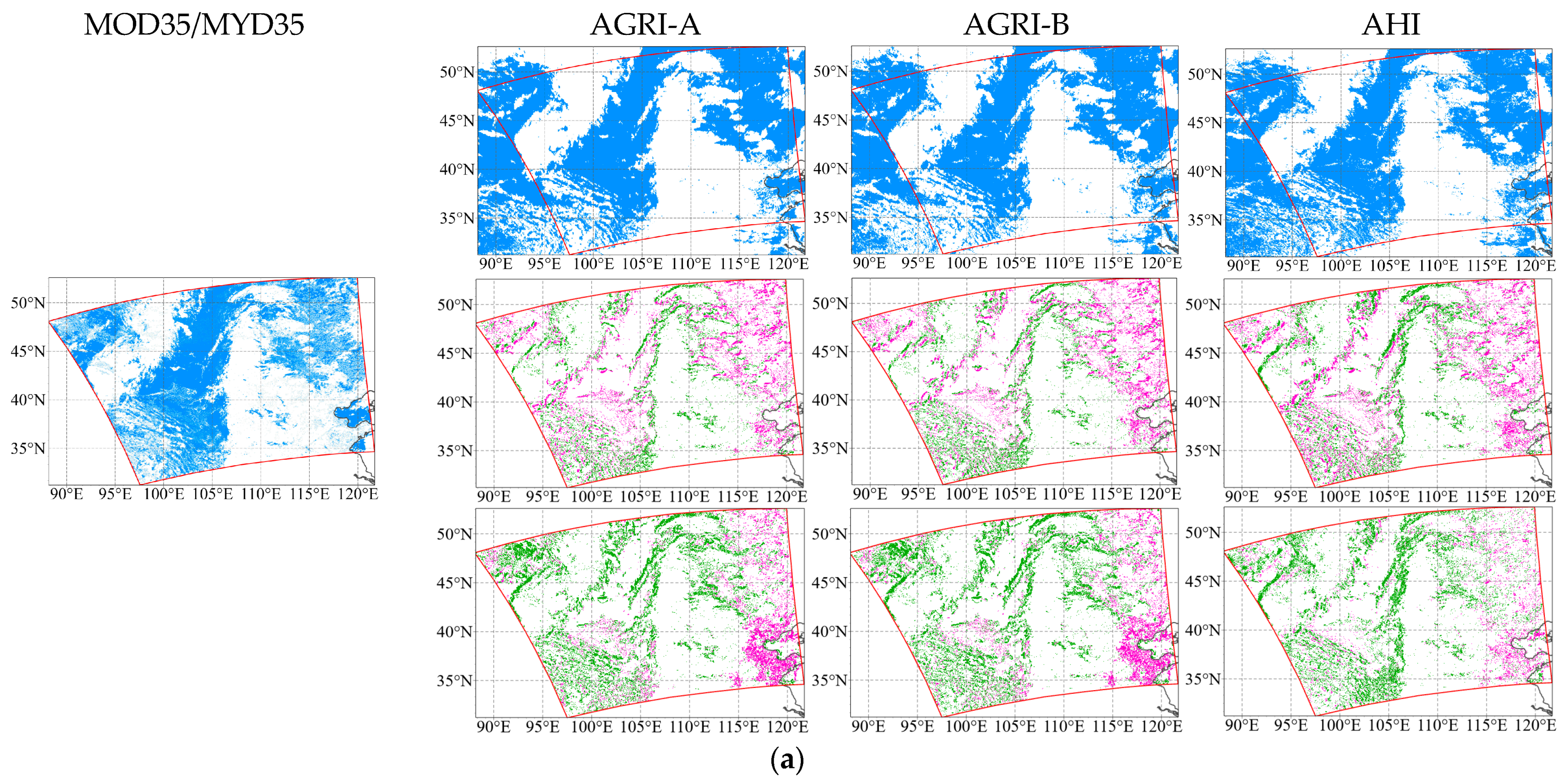
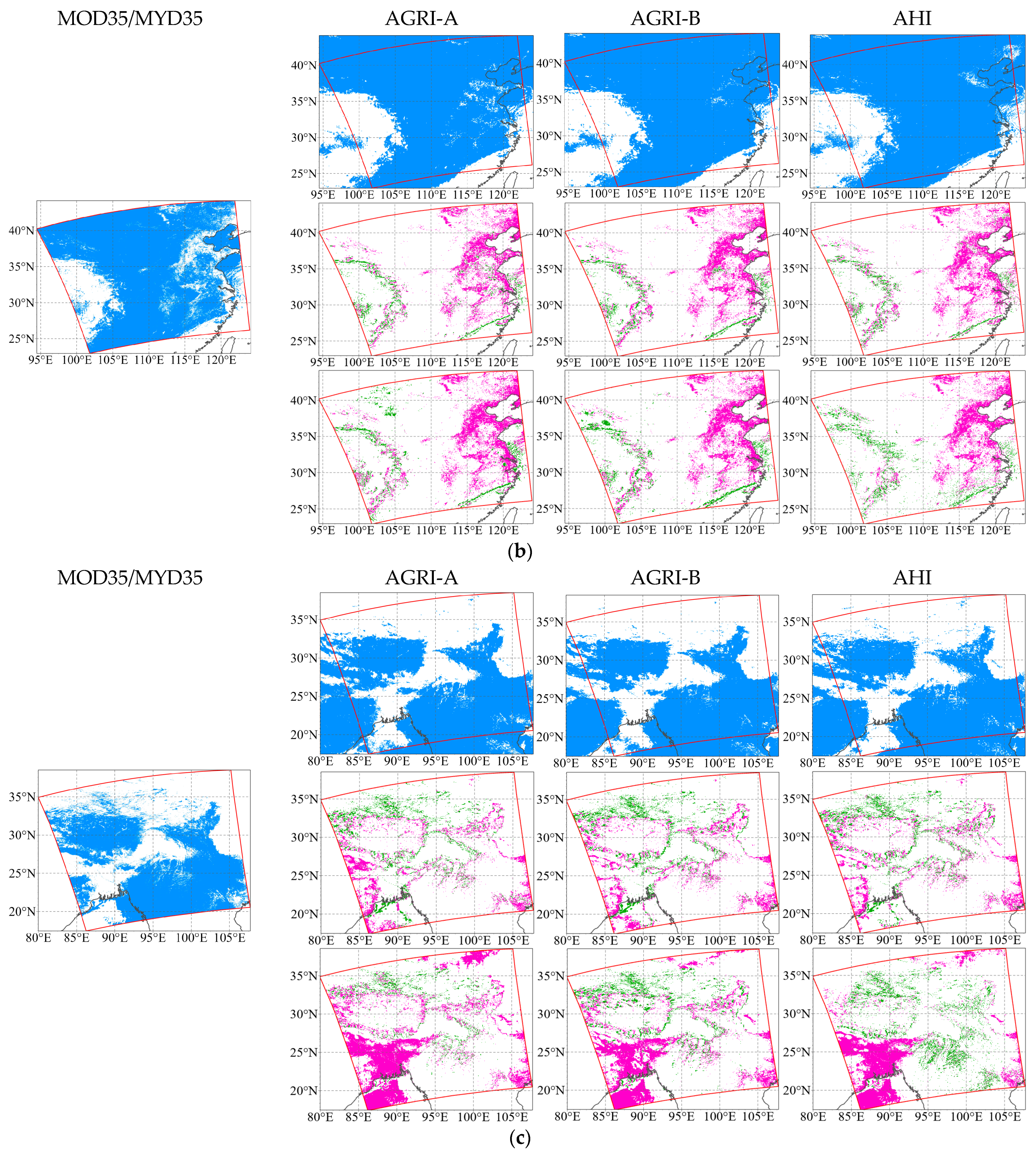
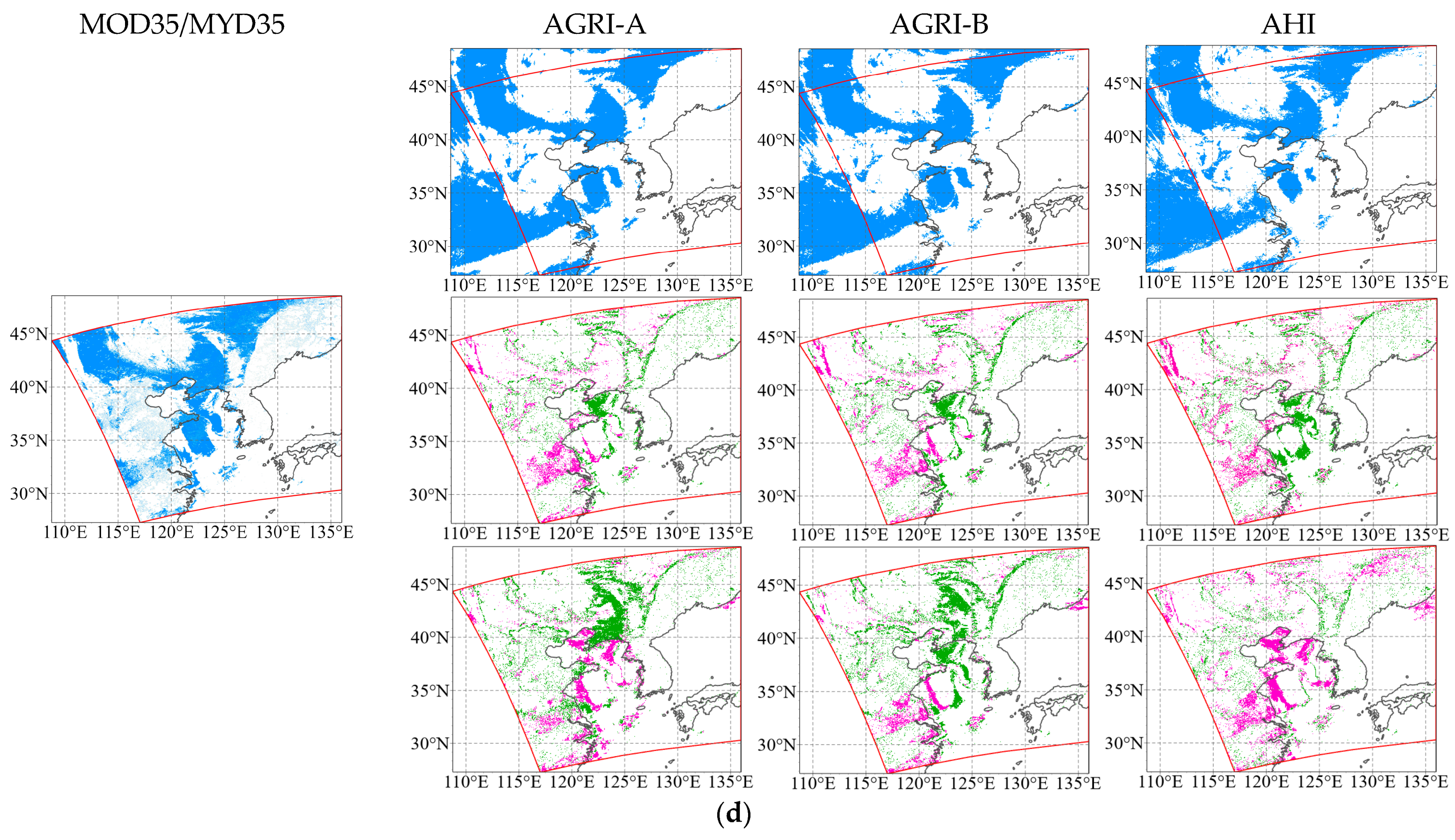
In order to further compare and evaluate the accuracy of the cloud mask results of AGRI-A, AGRI-B, and AHI, this study selects four cases of MODIS cloud at 6:00 on 2 July 2022 (a), 5:55 on 18 October 2022 (b), 7:00 on 13 January 2023 (c), and 5:00 on 15 April 2023 (d) mask product and the CALIOP product for three cases, 5 October 2022 at 6:00 (e), 11 March 2023 at 9:00 (f), and 6 May 2023 at 7:00 (g), were studied.
Figure 5 illustrates the cloud mask results for cases a, b, c, and d. To better highlight the differences between our results and the official products, we further present the discrepancies between MODIS and the TCM-CM, as well as between MODIS and three official cloud products: FY-4A CLM, FY-4B CLM, and H8/H9 CLP. Clearly, the TCM-CM results generated by AGRI-A, AGRI-B and AHI are very similar to each other in each case. This is consistent with the statistical characteristics of the MODIS validation results in Table 6. A visual comparison with the MODIS cloud mask reveals that the TCM-CM is slightly deficient in cloud and clear identification details, but the overall spatial distribution remains highly consistent with the MODIS cloud mask.
From the difference maps between MODIS and the cloud mask results, it can be observed that regardless of the case, the difference in pixel matching between the TCM-CM and MODIS cloud masks is consistently smaller than the difference between the official cloud products and MODIS, indicating that the TCM-CM misclassification rate for cloud and clear pixels is lower under MODIS validation. This demonstrates that our model outperforms the official products in terms of cloud mask.
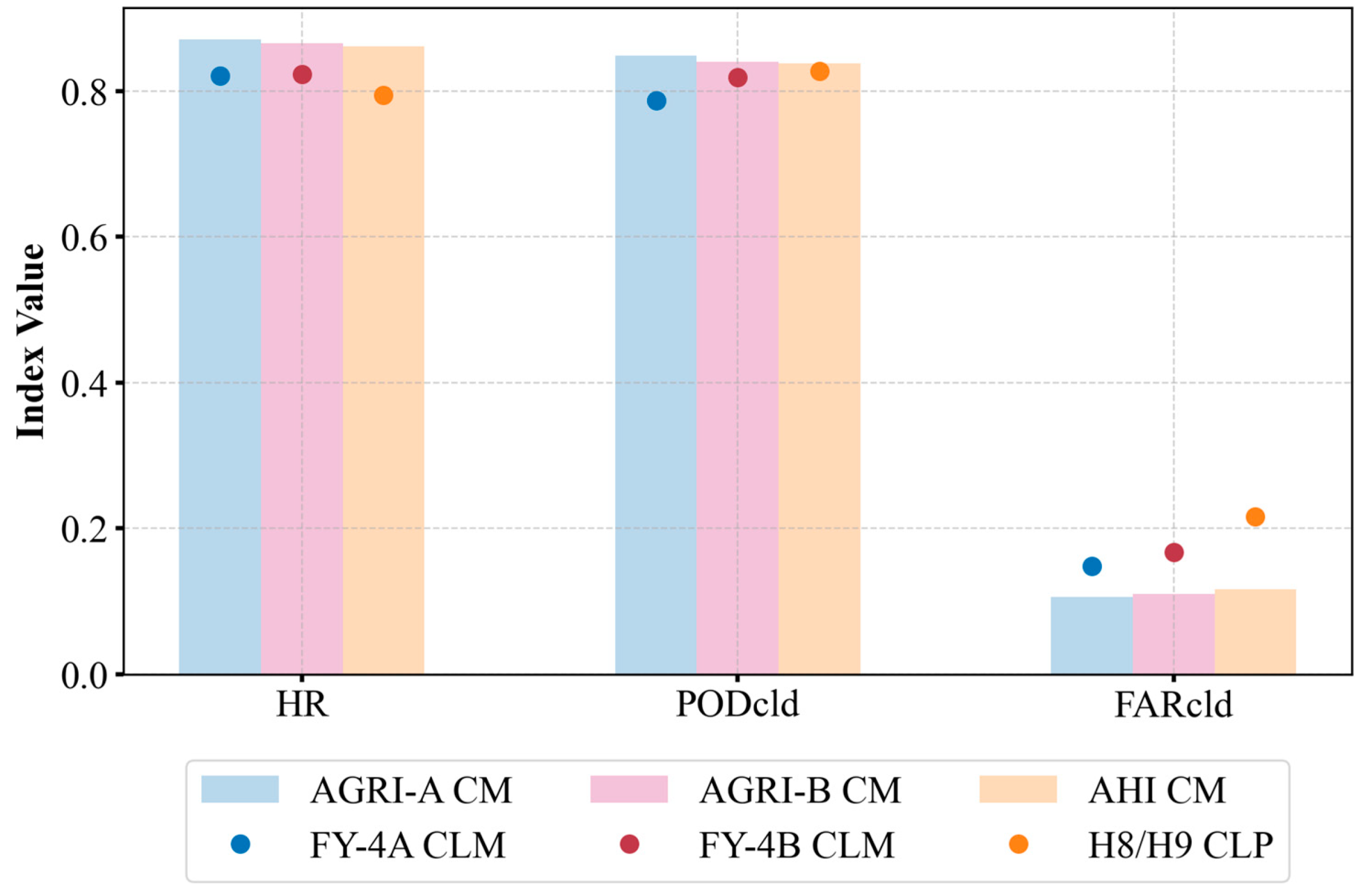
Table 7 summarizes the accuracy metrics based on MODIS data validation for the cases shown in Figure 5. The mean values are computed by merging the confusion matrices of all cases and calculating the metrics from the combined matrix. To present the metrics of the cases clearly and concisely, only HR, P O D c l d , and F A R c l d are shown. Although there are slight differences in the performance of TCM of AGRI-A, AGRI-B, and AHI in different cases, the ARGI-A CM still has the best performance with the highest HR, P O D c l d , and the lowest F A R c l d among all the cases. It is worth noting that for all cases, the HR of TCM-CM is higher than that of the official cloud products. Although the P O D c l d of the three official products in case a is higher, it is accompanied by higher F A R c l d , which lowers the HR.
Figure 6 compares the overall performance of the TCM-CM and official cloud products under MODIS validation from a visualization point of view. It can be clearly seen that the overall HR value is higher than the P O D c l d value, and TCM-CM outperforms the official product in both HR and P O D c l d , which verifies the stability and accuracy of its cloud recognition performance. AGRI-A performs the best, and AGRI-B is the second best. Analyzing from the perspective of official products, FY-4B CLM has higher overall HR, FY-4A CLM is the next best, while H8/H9 CLP has higher P O D c l d , but this is mainly at the expense of F A R c l d , reflecting a higher risk of misclassification in its cloud recognition.
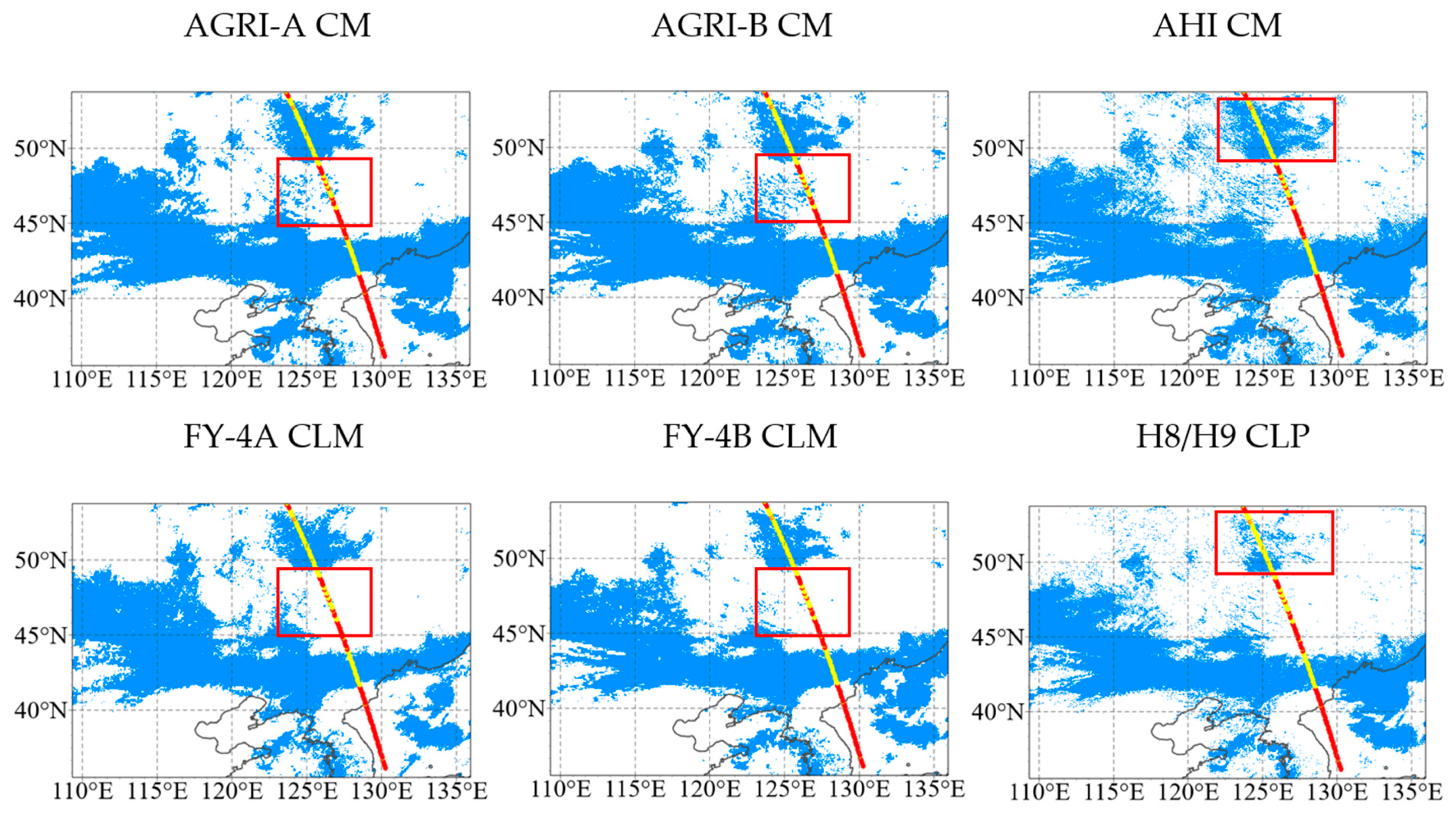
Table 8 lists the values of the metrics obtained from the validation of cases e, f, and g based on CALIOP data, and these values are computed over the entire area shown in the corresponding figures. The specific study of case e is shown in Figure 7. To facilitate a direct comparison, Figure 7 presents both the validation results of our TCM model (upper row) and the corresponding official cloud products (lower row). This helps clearly assess the differences between the TCM outputs and the official products under CALIOP validation. And the regions showing the most discernible differences are highlighted with red rectangles.
As demonstrated in Figure 7, a discernible discrepancy emerges between the AGRI-A CM, AGRI-B CM and AHI CM and the official cloud products. It can be demonstrated that in the upper region of the CALIOP data within the red rectangle, the AHI CM highly matches the CALIOP cloud mask; in the middle region of the CALIOP within the red rectangle, the FY-4A CLM and the FY-4B CLM determine almost all the pixels to be clouds, which significantly overestimates the range of the clouds. In contrast, the TCM-CM demonstrates a more precise and meticulous ability to identify clear pixels interspersed within the cloud pixels in this region, thereby exhibiting a superior cloud-clear discrimination capability. This phenomenon indicates that the official cloud product in case e has a more serious misclassification of cloud pixels.
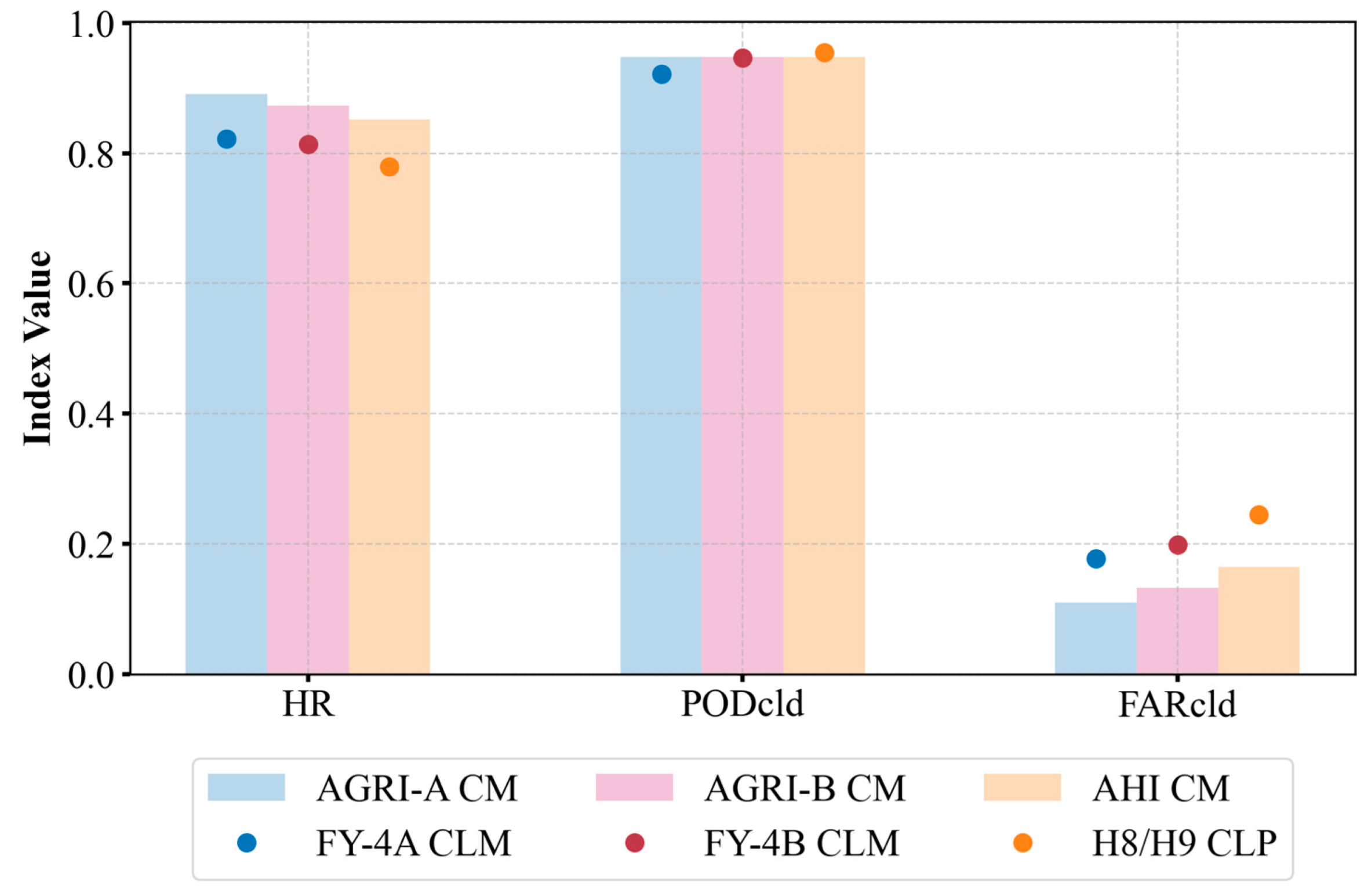
The above conclusion is also supported by the quantitative data in Table 8. In Table 8. Although the P O D c l d of the official cloud product in Case e reaches 1, which superficially shows a strong cloud detection ability, a large number of clear sky pixels are misclassified as cloudy. This leads to a significantly higher F A R c l d than that of the TCM-CM, almost double, resulting in a low overall HR and affecting the comprehensive performance of the cloud mask recognition. By contrast, the TCM-CM not only maintains a high P O D c l d under CALIOP validation, but also possesses a lower F A R c l d , and finally obtains a higher HR, which demonstrates its superiority in cloud recognition and is significantly better than the official products.
Figure 8 visualizes the performance of all CALIOP cases under each metric. It can be seen that the total HR of TCM-CM generated by each sensor performs similarly and stays around 0.85, regardless of the validation results based on MODIS or CALIOP. However, there is a significant difference in P O D c l d . The P O D c l d under CALIOP validation is generally as high as about 0.95, while the validation result from MODIS is only about 0.85. This phenomenon suggests that the TCM-CM are more responsive in cloud image recognition, but the higher cloud recognition may be accompanied by a slight lack of clear sky recognition.
In summary, both the case demonstration and the accuracy validation together show that the TCM-CM results demonstrate higher recognition accuracy and generalization ability across multiple source sensors.

4.3. Consistency Analysis

4.3.1. Variable Importance Analysis

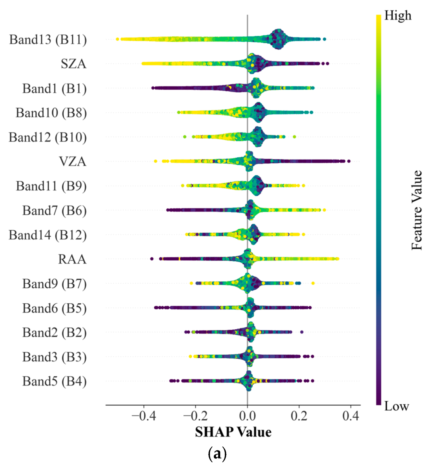
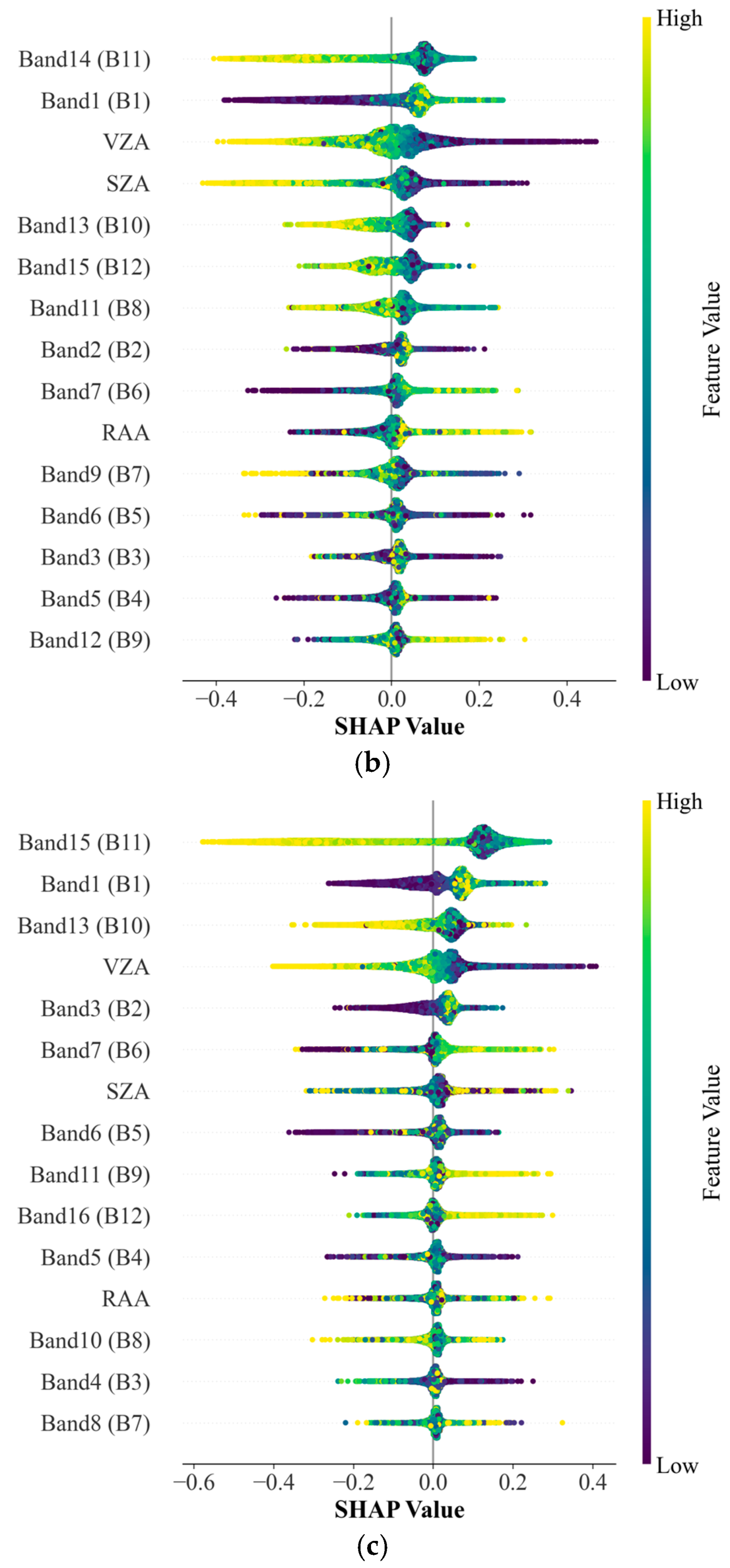
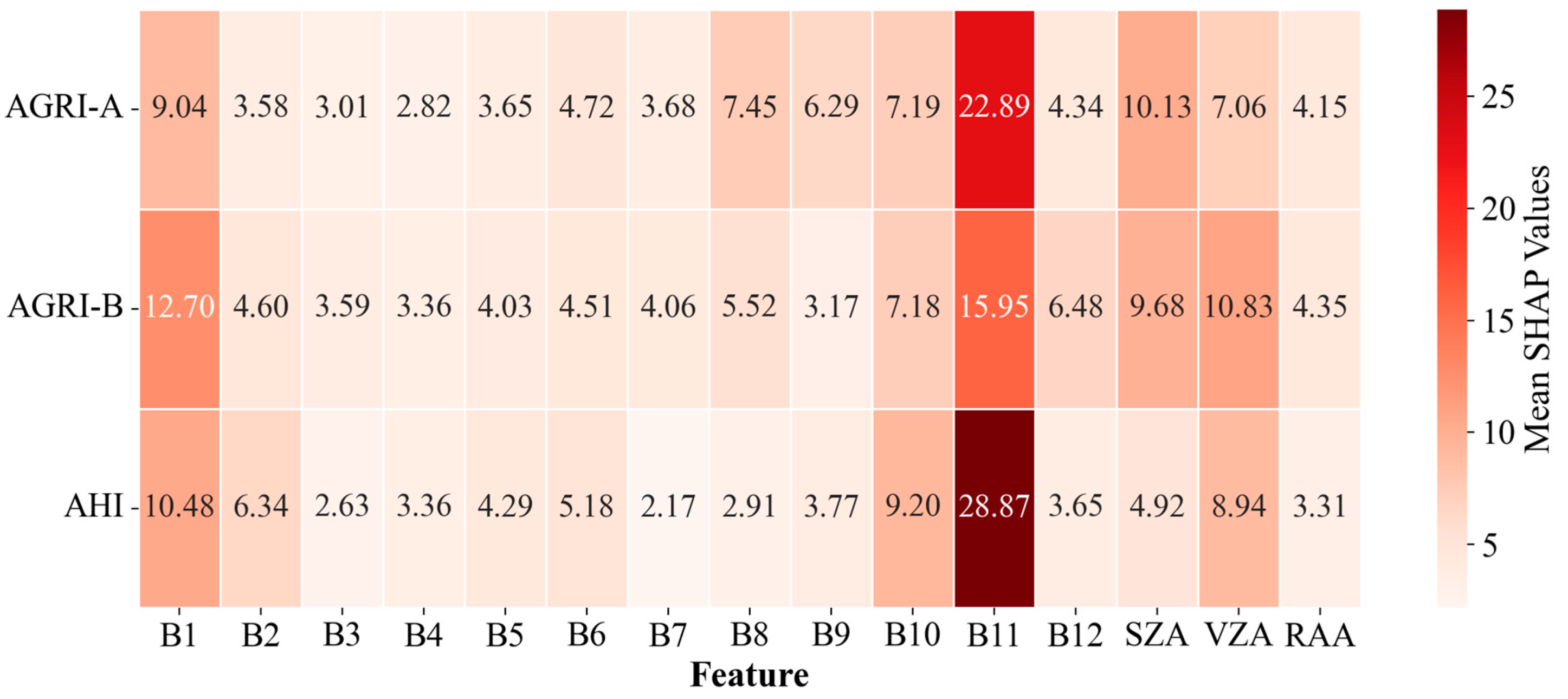
To measure the importance of each input feature to TCM cloud mask models, we calculated the mean absolute SHAP values of the TCM models of AGRI-A, AGRI-B, and AHI (Table 9). Since the sum of mean SHAP values across features is not a fixed constant, we normalized the mean SHAP values to enable a fair comparison of feature contributions among the three cloud mask models.
The channel B11 (12.0–12.4 µm) is the dominant feature across all models, with contributions ranging from 15.95% to 28.87%, indicating its key role in cloud identification. This is physically consistent because B11 is highly sensitive to the thermal contrast between typically cold cloud tops and the warmer Earth’s surface, which is a fundamental mechanism for detecting clouds in the thermal infrared [41,48]. The B1 (0.47 µm) channel also exhibits high importance (9.04–12.8%). The B1 channel captures reflected solar radiation, which is critical for identifying daytime clouds and distinguishing them from bright surfaces such as snow or desert [49]. The AGRI-A model maintains a relatively balanced dependence on each feature, while AGRI-B exhibits a feature bias. The AHI model strongly relies on the B11 band but also incorporates other auxiliary features. Additionally, geometric features such as SZA and VZA contribute significantly in almost all models, accounting for up to 10.83%.
To further explore the role of features about the model output values, the positive and negative effects of TCM model features for AGRI-A, AGRI-B, and AHI are discussed in this study via SHAP summary plots (Figure 9). Figure 9 complements Table 9 by illustrating the distribution of SHAP values for individual samples, thereby revealing the variability and density of feature contributions. The channel B11, as well as the geometric features SZA and VZA, exhibit a consistent trend of influence, contributing positively to the predictions when these features have low values, making it easier for the model to identify cloud pixels. This is consistent with the physical property that clouds usually have lower brightness temperatures, and the imaging is clearer at smaller geometric observation angles, which facilitates observation. Conversely, when these eigenvalues are higher, their positive contributions to the prediction gradually weaken or even turn negative. This indicates that it becomes more difficult to discriminate between clouds and the background under high brightness temperature or extreme observation angle conditions. Consequently, the prediction accuracy of the cloud mask decreases. Meanwhile, the visible channel B1 shows an opposite trend of influence: the higher its eigenvalue, the stronger the positive effect on the model prediction. This indicates that under daytime conditions, the high reflectivity of clouds in channel B1 significantly enhances the brightness contrast between clouds and background, thus improving the model’s ability to recognize cloud pixels. In conclusion, the SHAP analysis reveals the correspondence between the behavioral patterns of each key feature and the physical mechanisms, further validating the effective use of multi-source information by the TCM model.

4.3.2. Variability Analysis

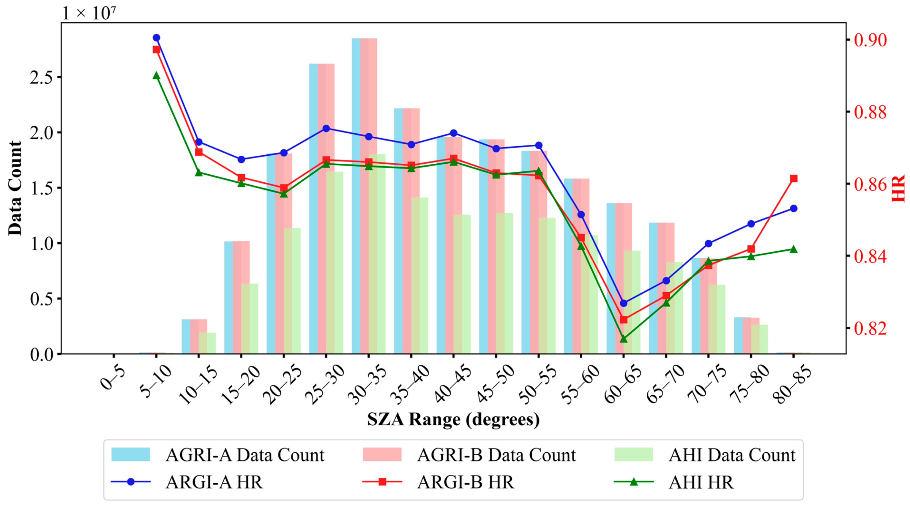
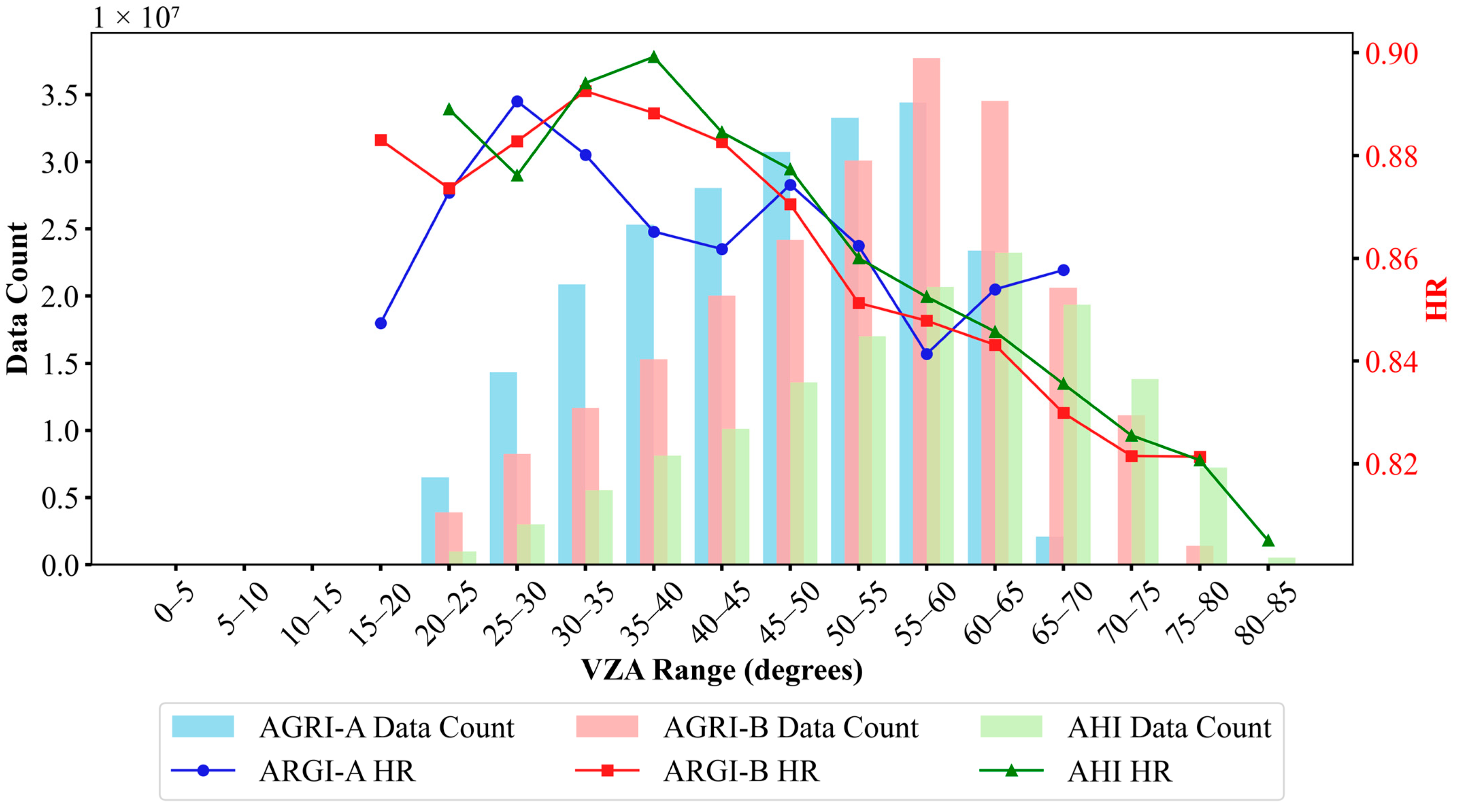
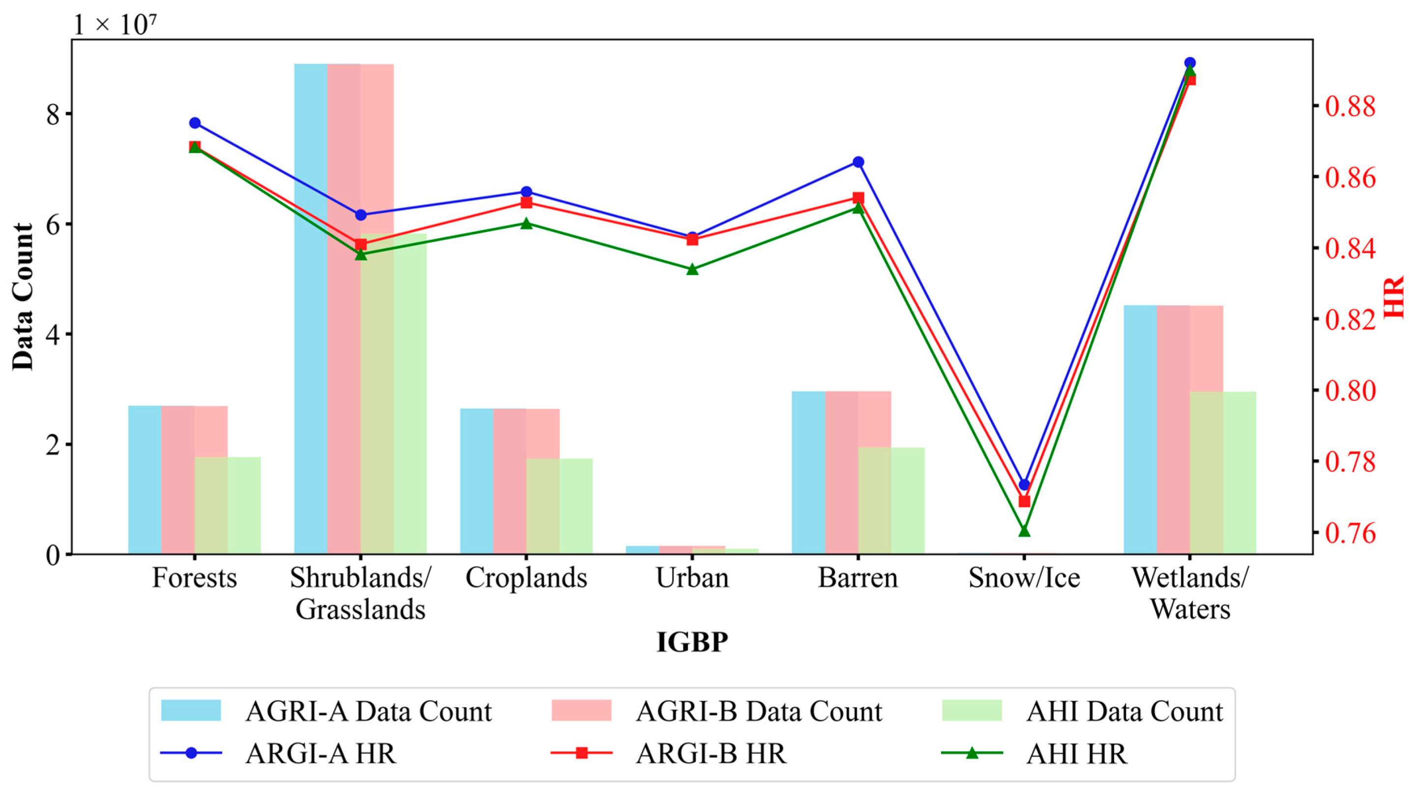
We calculated the classification accuracies and counts of pixels of different sensors for different SZA, VZA, and surface types scenarios using MOD35/MYD35 as a baseline to discern the variation pattern between the cloud mask hit rate and the variation in the influencing factors. With MOD35/MYD35 data as a reference, the matching counts and accuracies of the TCM-CM from AGRI-A, AGRI-B, and AHI under varying ranges of SZA and VZA as well as for different IGBP are shown in Figure 10, Figure 11 and Figure 12.
As can be seen from Figure 10, the sensors exhibit a consistent trend across different SZA ranges. In the 10–55° range, the HR of the TCM-CM in all sensors remain relatively stable, maintaining a value of around 0.86. However, when the SZA is larger than 55°, the accuracy decreases significantly. This phenomenon suggests that the cloud boundary becomes blurred due to the weakened radiance contrast between the surface and the clouds at high SZA, leading to degradation of model recognition performance. The high HR at SZA less than 10° and the rise in HR above 65° may be related to the small matching counts. Overall, AGRI-A maintains a consistently high HR in all SZA intervals, showing stronger adaptability to solar illumination angles and reliable cloud identification. Meanwhile the HR of AGRI-B and AHI exhibit significant overlap.
The VZA determines the degree of distortion of the remote sensing image. In general, the more severe the stretching of the pixels by the sensor observation (i.e., the larger the VZA), the lower the observation accuracy. As shown in Figure 11, the cloud mask accuracy of all sensors uniformly shows an increasing and then decreasing trend as VZA increases. For AGRI-B and AHI, the HR gradually decreases when VZA exceeds 30° and 40°, respectively, indicating that larger observation angles increase the atmospheric path length and the degree of cloud boundary distortion, affecting the model identification accuracy. In regions where the VZA is less than 45°, the HR of each sensor remains high, around 0.88. Notably, in the medium-high VZA interval (30°~60°), the HR of AGRI-B slightly outperforms the other two models, demonstrating its relative adaptability to the tilted viewing angles. By comparison, the HR of the TCM-CM from AGRI-A exhibits pronounced fluctuations within the SZA range of 15–70°.
It is noteworthy that full-sample validation based on CALIOP and MODIS in Section 4.1 shows that the cloud mask classification accuracy of AHI is always lower than that of AGRI-A and AGRI-B. However, in Figure 11, when the VZA is controlled within the same range for comparison, AHI exhibits higher HR values than the other sensors across several angular intervals. This phenomenon indicates that the unbalanced distribution of VZA introduces systematic bias. Moreover, VZA is also one of the key factors affecting the cloud mask performance of AHI: its detection accuracy is limited under large angle conditions, whereas its performance is better at low to medium angles. This further highlight that, in the cross-validation of multi-source remote sensing data, observational geometry must be fully considered to mitigate the interference in performance assessment results and to avoid misinterpretation or bias caused by viewing angle differences.
The difference in accuracy of cloud masks on different surface types is closely related to the influence of surface features on the cloud optical or thermal properties. Figure 12 shows the count of matched pixels versus cloud mask accuracy for each sensor for different IGBP surface reclassifications. Consistent with SZA, the variation patterns of different IGBP show similar trends. The results show that in the Snow/Ice region, the HR of all sensors drop significantly, down to 0.76. This is mainly because the high albedo characteristics of this type of surface are similar to the spectral properties of clouds in the visible and infrared channels, leading to recognition confusion. On the contrary, wetlands/waters and barren usually have low albedo in the visible and shortwave infrared channels, contrasting starkly with the high albedo characteristics of clouds. This results in a higher recognition accuracy for the TCM model, reaching over 0.88, which reflects the high dependence of the cloud mask algorithm on the surface type. In addition, the TCM model can achieve stable high-accuracy classification in forests, shrublands/grasslands, croplands, and urban areas with varying numbers of matched pixels. This indicates that the TCM model is not dependent on a single channel or a fixed threshold, and demonstrates its adaptability and robustness to different surfaces. Overall, the HR of AGRI-A are consistently higher than those of AGRI-B and AHI for most surface types, suggesting that its model has a greater capacity to recognize cloud and generalize to complex surface backgrounds.

5. Discussion

5.1. Performance of TCM, MCM, and CCM by IGBP Class

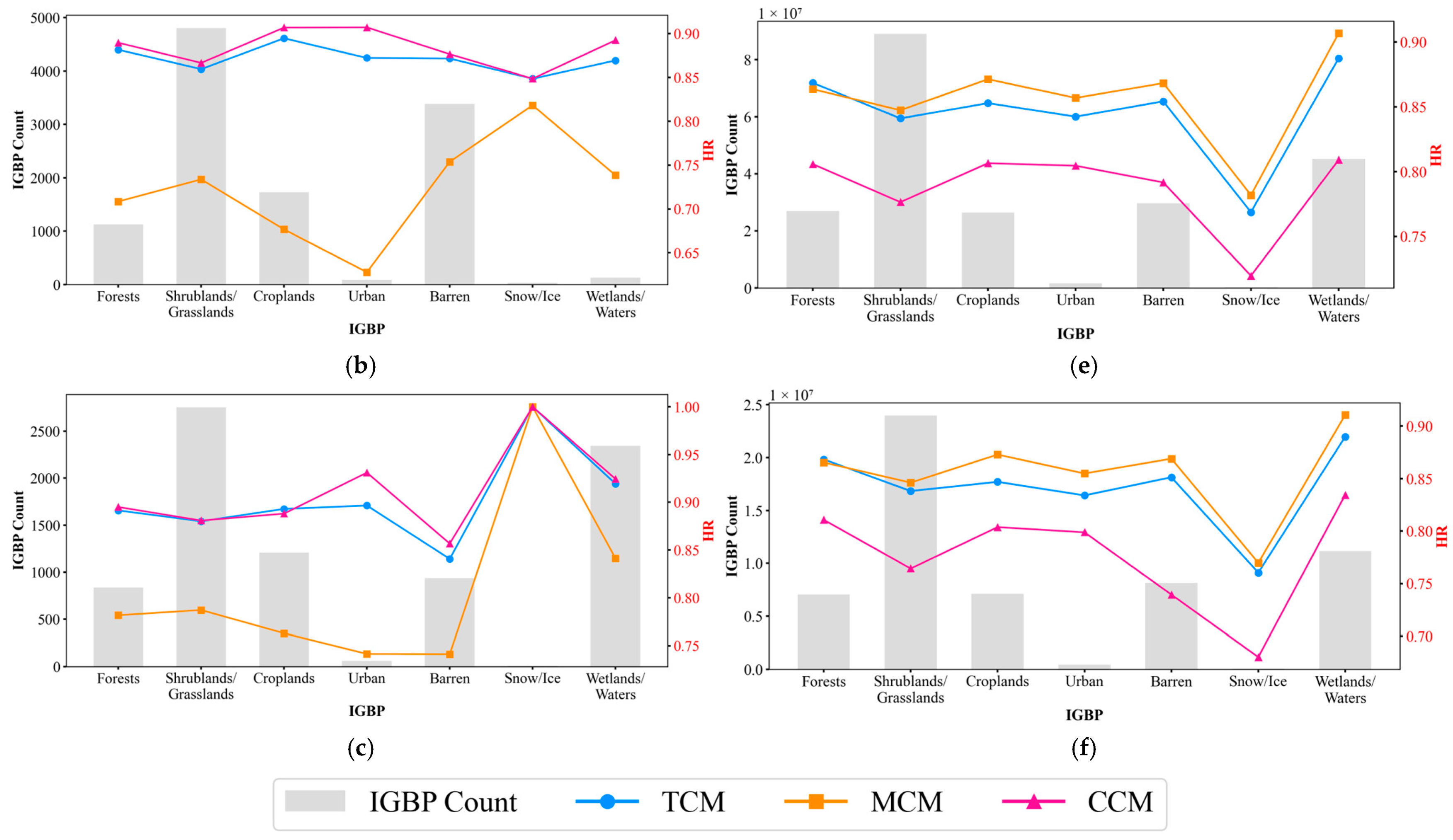
To evaluate regional differences in the performance of TCM, MCM, and CCM, we compared their cloud detection accuracies across various IGBP surface types using both CALIPSO VFM and MOD35/MYD35 as reference datasets (Figure 13). Under CALIPSO validation, TCM achieves accuracy comparable to that of CCM, whereas under MODIS validation, TCM performs similarly to MCM. These patterns are consistent with the overall results shown in Figure 3 and Figure 4, highlighting that TCM remains robust and effective across diverse surface types. In addition, the accuracy over snow/ice surfaces is generally higher when validated against CALIPSO than when validated against MODIS. This discrepancy is likely attributed to the relatively limited number of snow/ice pixels in the CALIOP reference dataset, which reduces the diversity of sampled surface and atmospheric conditions. Nevertheless, this limitation does not diminish the transferability of TCM, as its robustness is consistently demonstrated across different surface types and validation datasets, and sensors.

5.2. Comparison of Mean SHAP Values and RF Feature Importance Scores

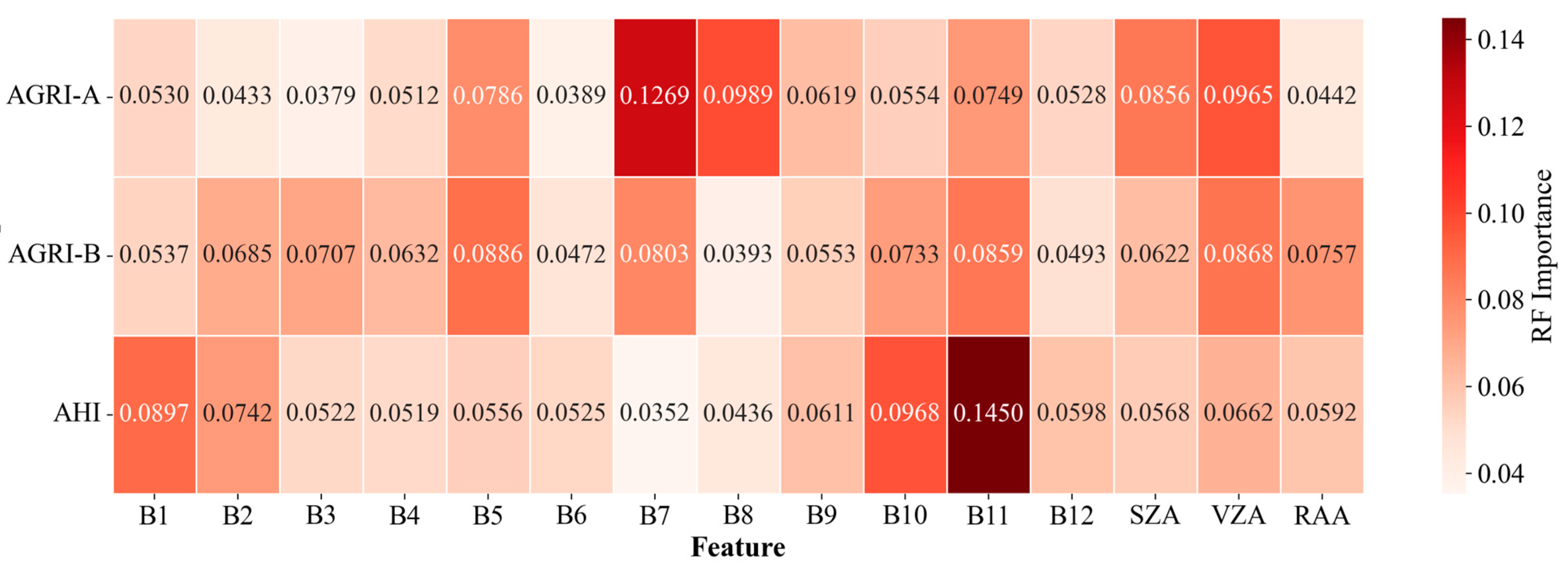
A comparative analysis was conducted between mean absolute SHAP values and standard RF feature importance scores to validate the interpretability of our models. The Normalized mean SHAP values heatmap presented in Figure 14 is generated based on the results in Table 9, while the RF importance scores are shown in Figure 15. As can be seen, SHAP contributions are largely consistent across the three models (TCM for AGRI-A, AGRI-B, and AHI), indicating similar effects of spectral bands and angular features on model outputs. In contrast, RF importance rankings differ noticeably: AGRI-A emphasizes B7 and B8, AGRI-B highlights B5 and VZA, and AHI prioritizes B11 and B10. Such discrepancies are attributable to the inherent methodological limitations of the Gini importance used by RF, which is known to be biased and can produce unreliable attributions when features exhibit multicollinearity—a common characteristic of multi-spectral remote sensing data [50,51]. In contrast, SHAP is grounded in game theory and provides a more robust and theoretically sound feature attribution by evaluating the marginal contribution of each feature across all possible feature coalitions, thus handling collinearity more effectively [47]. Consequently, the interpretations and conclusions presented in this study are therefore based on the more reliable SHAP analysis.

5.3. Limitations and Future Work

Several aspects of our study warrant further investigation. Our models achieved satisfactory results for daytime cloud detection across AGRI-A, AGRI-B, and AHI. Future work will extend this analysis to include nighttime observations and will also explore the generalizability of our approach to other geostationary sensors, such as GOES-R/ABI.
Second, our training and testing relied on 1% of the matched MODIS samples, which, despite representing approximately 200 million data points, may introduce sampling bias for rare or extreme cloud conditions. Future studies will explore larger or stratified sampling to better assess potential biases and uncertainty propagation.
Third, the reference products (MOD35/MYD35 and CALIPSO VFM) have inherent uncertainties, arising from surface reflectance effects, thin cloud detection limits, or sensor coverage constraints. Quantifying these uncertainties, for example, through high-quality ground-based observations, will be considered in future work.
Fourth, geometric factors such as satellite zenith angle (VZA) can introduce inconsistencies in model performance, as observed in AGRI-A and AHI. In future work, we plan to investigate strategies to correct these angle-dependent effects. Addressing such geometric biases is an important aspect of satellite-based cloud detection to ensure robust and consistent results across different viewing geometries.
These considerations highlight several promising directions for extending the robustness, representativeness, and general applicability of our cloud detection framework.

6. Conclusions

In order to solve the problems that current cloud mask studies mostly focus on a single sensor and commonly used reference data such as CALIOP and MODIS cloud products have limited spatial coverage or insufficient sensitivity to vertical structures, this study proposes to use a unified cloud mask algorithm framework (TCM) to conduct a systematic study on cloud mask detection and the consistency analysis of the detection results for typical geostationary orbit satellite sensors FY-4A/AGRI, FY-4B/AGRI and Himawari-8/9 AHI. The main conclusions are as follows.
The TCM algorithm maintains the leading position in both CALIOP and MODIS validation, with HR values higher than 0.85 and P O D c l d above 0.89, which fully reflects the effectiveness of TrAdaBoost migration learning strategy in target domain modeling and cross-domain generalization.
The cross-validation results with multi-source data show that the accuracy of TCM cloud mask results is better than the official cloud products of FY-4A CLM, FY-4B CLM, and H8/H9 CLP. On average across all cases, the TCM-CM from AGRI-A is always the most stable under different evaluation criteria, with the highest HR, and lowest F A R c l d . The TCM algorithm demonstrated excellent classification performance and generalization ability. The TCM model of AHI has relatively low accuracy in all evaluations, but its performance is significantly improved under the same VZA conditions, indicating that it is greatly affected by the observation geometry conditions.
SHAP interpretable analysis reveals that the 0.47 μm visible channel, the 10.8/10.4 μm and 12.0/12.4 μm infrared channels, as well as the geometrical features SZA, VZA, etc., significantly influence the TCM-CM. The variability analysis shows that all sensors exhibit high consistency in the SZA and IGBP dimensions. This indicates that the response of each sensor to the lighting conditions and surface background is more consistent under the framework of TCM algorithm which has good cross-platform adaptability. Meanwhile, it is further illustrated that under the premise of controlling the observation geometry difference, the multi-source geostationary satellite cloud mask product has strong fusion potential, which lays the foundation for the integrated application of multi-source satellite datasets.
Comprehensively, our research results validate the effectiveness and stability of TrAdaboost, which not only provides a quantitative basis for the consistency assessment of multi-source satellite cloud mask detection, but also provides a theoretical basis and technical support for geostationary satellite dataset integration applications and high-precision cloud detection.

Author Contributions

Conceptualization, L.F., M.Z. and W.Q.; methodology, C.H. and Z.W.; software, C.H. and Q.L.; validation, Z.W., Q.L., L.F., M.Z. and L.W.; formal analysis, C.H., Z.W., Q.L. and L.F.; investigation, C.H., Z.W., M.T. and Y.W.; data curation, C.H. and L.W.; writing—original draft preparation, C.H. and Z.W.; writing—review and editing, Z.W., Q.L., L.F., W.Q., M.Z., M.T., Y.W. and L.W.; project administration, L.F. and L.W.; funding acquisition, L.F. and L.W. All authors have read and agreed to the published version of the manuscript.

Funding

This work was financially supported by the National Natural Science Foundation of China (42375129, 42371354, and 41975036), Fundamental Research Funds for the National University, China University of Geosciences, Wuhan (2024XLA57).

Data Availability Statement

The data presented in this study are available on request from the corresponding author and first author.

Acknowledgments

The authors would like to thank National Aeronautics and Space Administration, China Meteorological Administration and Japan Meteorological Agency for providing MODIS, CALIOP, Fengyun-4 and Himawari-8/9 datasets.

Conflicts of Interest

The authors declare no conflicts of interest.

Abbreviations

The following abbreviations are used in this manuscript:
TCMTrAdaBoost cloud mask algorithm
MCMMODIS-based cloud mask algorithm
CCMCALIOP-based cloud mask algorithm
TCM-CMCloud mask results generated by the TCM algorithm from each sensor
AGRI-AFY-4A/AGRI
AGRI-BFY-4B/AGRI
AHIHimawair-8 AHI and Himawair-9 AHI
AGRI-A CMCloud mask results generated by the TCM algorithm from AGRI-A
AGRI-B CMCloud mask results generated by the TCM algorithm from AGRI-B
AHI CMCloud mask results generated by the TCM algorithm from AHI
B10.47 μm band of AGRI-A, AGRI-B and AHI
B20.65 μm band of AGRI-A and AGRI-B; 0.64 μm band of AHI
B30.83 μm band of AGRI-A; 0.825 μm band of AGRI-B; 0.86 μm band of AHI
B41.61 μm band of AGRI-A and AGRI-B; 1.6 μm band of AHI
B52.22 μm band of AGRI-A; 2.225 μm band of AGRI-B; 2.3 μm band of AHI
B63.72 μm band of AGRI-A; 3.75 μm band of AGRI-B; 3.9 μm band of AHI
B76.25 μm band of AGRI-A and AGRI-B; 6.2 μm band of AHI
B87.10 μm band of AGRI-A; 7.42 μm band of AGRI-B; 7.3 μm band of AHI
B98.50 μm band of AGRI-A; 8.55 μm band of AGRI-B; 8.6 μm band of AHI
B1010.80 μm band of AGRI-A and AGRI-B; 10.4 μm band of AHI
B1112.0 μm band of AGRI-A and AGRI-B; 12.4 μm band of AHI
B1213.5 μm band of AGRI-A; 13.3 μm band of AGRI-B and AHI
SZASolar zenith angle
VZASatellite zenith angle
RAARelative azimuthal angle
PODProbability of detection
FARFalse alarm ratio
HRHit rate
KSSKuiper’s skill score

References

  1. Baker, M.B. Cloud Microphysics and Climate. Science 1997, 276, 1072–1078. [Google Scholar] [CrossRef]
  2. Shen, X.; Li, Q.; Tian, Y.; Shen, L. An Uneven Illumination Correction Algorithm for Optical Remote Sensing Images Covered with Thin Clouds. Remote Sens. 2015, 7, 11848–11862. [Google Scholar] [CrossRef]
  3. Tapakis, R.; Charalambides, A.G. Equipment and methodologies for cloud detection and classification: A review. Sol. Energy 2013, 95, 392–430. [Google Scholar] [CrossRef]
  4. Li, X.; Wang, L.; Cheng, Q.; Wu, P.; Gan, W.; Fang, L. Cloud removal in remote sensing images using nonnegative matrix factorization and error correction. ISPRS J. Photogramm. Remote Sens. 2019, 148, 103–113. [Google Scholar] [CrossRef]
  5. Shen, H.; Li, H.; Qian, Y.; Zhang, L.; Yuan, Q. An effective thin cloud removal procedure for visible remote sensing images. ISPRS J. Photogramm. Remote Sens. 2014, 96, 224–235. [Google Scholar] [CrossRef]
  6. Platnick, S.; Meyer, K.G.; King, M.D.; Wind, G.; Amarasinghe, N.; Marchant, B.; Arnold, G.T.; Zhang, Z.; Hubanks, P.A.; Holz, R.E. The MODIS cloud optical and microphysical products: Collection 6 updates and examples from Terra and Aqua. IEEE Trans. Geosci. Remote Sens. 2016, 55, 502–525. [Google Scholar] [CrossRef]
  7. Zhu, Z.; Woodcock, C.E. Automated cloud, cloud shadow, and snow detection in multitemporal Landsat data: An algorithm designed specifically for monitoring land cover change. Remote Sens. Environ. 2014, 152, 217–234. [Google Scholar] [CrossRef]
  8. Chepfer, H.; Bony, S.; Winker, D.; Chiriaco, M.; Dufresne, J.L.; Sèze, G. Use of CALIPSO lidar observations to evaluate the cloudiness simulated by a climate model. Geophys. Res. Lett. 2008, 35, L15704. [Google Scholar] [CrossRef]
  9. Kotarba, A.Z. Calibration of global MODIS cloud amount using CALIOP cloud profiles. Atmos. Meas. Tech. 2020, 13, 4995–5012. [Google Scholar] [CrossRef]
  10. Zhu, Z.; Wang, S.; Woodcock, C.E. Improvement and expansion of the Fmask algorithm: Cloud, cloud shadow, and snow detection for Landsats 4–7, 8, and Sentinel 2 images. Remote Sens. Environ. 2015, 159, 269–277. [Google Scholar] [CrossRef]
  11. Chen, N.; Li, W.; Gatebe, C.; Tanikawa, T.; Hori, M.; Shimada, R.; Aoki, T.; Stamnes, K. New neural network cloud mask algorithm based on radiative transfer simulations. Remote Sens. Environ. 2018, 219, 62–71. [Google Scholar] [CrossRef]
  12. Li, Z.; Shen, H.; Cheng, Q.; Liu, Y.; You, S.; He, Z. Deep learning based cloud detection for medium and high resolution remote sensing images of different sensors. ISPRS J. Photogramm. Remote Sens. 2019, 150, 197–212. [Google Scholar] [CrossRef]
  13. Wang, C.; Platnick, S.; Meyer, K.; Zhang, Z.; Zhou, Y. A machine-learning-based cloud detection and thermodynamic-phase classification algorithm using passive spectral observations. Atmos. Meas. Tech. 2020, 13, 2257–2277. [Google Scholar] [CrossRef]
  14. Frantz, D.; Haß, E.; Uhl, A.; Stoffels, J.; Hill, J. Improvement of the Fmask algorithm for Sentinel-2 images: Separating clouds from bright surfaces based on parallax effects. Remote Sens. Environ. 2018, 215, 471–481. [Google Scholar] [CrossRef]
  15. Shang, H.; Letu, H.; Xu, R.; Wei, L.; Wu, L.; Shao, J.; Nagao, T.M.; Nakajima, T.Y.; Riedi, J.; He, J. A hybrid cloud detection and cloud phase classification algorithm using classic threshold-based tests and extra randomized tree model. Remote Sens. Environ. 2024, 302, 113957. [Google Scholar] [CrossRef]
  16. Wei, J.; Huang, W.; Li, Z.; Sun, L.; Zhu, X.; Yuan, Q.; Liu, L.; Cribb, M. Cloud detection for Landsat imagery by combining the random forest and superpixels extracted via energy-driven sampling segmentation approaches. Remote Sens. Environ. 2020, 248, 112005. [Google Scholar] [CrossRef]
  17. Choi, Y.-J.; Han, H.-J.; Hong, S. A daytime cloud detection method for advanced meteorological imager using visible and near-infrared bands. IEEE Trans. Geosci. Remote Sens. 2023, 61, 1–13. [Google Scholar] [CrossRef]
  18. Gao, F.; Masek, J.; Schwaller, M.; Hall, F. On the blending of the Landsat and MODIS surface reflectance: Predicting daily Landsat surface reflectance. IEEE Trans. Geosci. Remote Sens. 2006, 44, 2207–2218. [Google Scholar] [CrossRef]
  19. Zheng, X.; Yu, J.; Han, L. Research on PWV calculation combining MODIS and ERA5. In Proceedings of the Fourth International Conference on Geology, Mapping, and Remote Sensing (ICGMRS 2023), Wuhan, China, 14–16 April 2023; pp. 72–78. [Google Scholar]
  20. Yi, B.; Rapp, A.D.; Yang, P.; Baum, B.A.; King, M.D. A comparison of Aqua MODIS ice and liquid water cloud physical and optical properties between collection 6 and collection 5.1: Pixel-to-pixel comparisons. J. Geophys. Res. Atmos. 2017, 122, 4528–4549. [Google Scholar] [CrossRef]
  21. Yi, B.; Rapp, A.D.; Yang, P.; Baum, B.A.; King, M.D. A comparison of Aqua MODIS ice and liquid water cloud physical and optical properties between collection 6 and collection 5.1: Cloud radiative effects. J. Geophys. Res. Atmos. 2017, 122, 4550–4564. [Google Scholar] [CrossRef]
  22. Lai, R.; Teng, S.; Yi, B.; Letu, H.; Min, M.; Tang, S.; Liu, C. Comparison of cloud properties from Himawari-8 and FengYun-4A geostationary satellite radiometers with MODIS cloud retrievals. Remote Sens. 2019, 11, 1703. [Google Scholar] [CrossRef]
  23. Frey, R.A.; Ackerman, S.A.; Holz, R.E.; Dutcher, S.; Griffith, Z. The continuity MODIS-VIIRS cloud mask. Remote Sens. 2020, 12, 3334. [Google Scholar] [CrossRef]
  24. Wang, X.; Min, M.; Wang, F.; Guo, J.; Li, B.; Tang, S. Intercomparisons of cloud mask products among Fengyun-4A, Himawari-8, and MODIS. IEEE Trans. Geosci. Remote Sens. 2019, 57, 8827–8839. [Google Scholar] [CrossRef]
  25. King, M.D.; Platnick, S.; Menzel, W.P.; Ackerman, S.A.; Hubanks, P.A. Spatial and temporal distribution of clouds observed by MODIS onboard the Terra and Aqua satellites. IEEE Trans. Geosci. Remote Sens. 2013, 51, 3826–3852. [Google Scholar] [CrossRef]
  26. Li, E.; Zhang, Z.; Tan, Y.; Wang, Q. A novel cloud detection algorithm based on simplified radiative transfer model for aerosol retrievals: Preliminary result on Himawari-8 over eastern China. IEEE Trans. Geosci. Remote Sens. 2020, 59, 2550–2561. [Google Scholar] [CrossRef]
  27. Wang, K.; Wang, F.; Lu, Q.; Liu, R.; Zheng, Z.; Wang, Z.; Wu, C.; Ni, Z.; Liu, X. Algorithm for detecting ice overlaying water multilayer clouds using the infrared bands of FY-4A/AGRI. IEEE Geosci. Remote Sens. Lett. 2024, 21, 1001205. [Google Scholar] [CrossRef]
  28. Wilson, M.J.; Oreopoulos, L. Enhancing a simple MODIS cloud mask algorithm for the Landsat data continuity mission. IEEE Trans. Geosci. Remote Sens. 2012, 51, 723–731. [Google Scholar] [CrossRef]
  29. Tan, S.; Zhang, X.; Shi, G. MODIS cloud detection evaluation using CALIOP over polluted eastern China. Atmosphere 2019, 10, 333. [Google Scholar] [CrossRef]
  30. Ahmad, M.; Mauro, F.; Raza, R.A.; Mazzara, M.; Distefano, S.; Khan, A.M.; Ullo, S.L. Transformer-Driven Active Transfer Learning for Cross-Hyperspectral Image Classification. IEEE J. Sel. Top. Appl. Earth Obs. Remote Sens. 2025, 18, 19635–19648. [Google Scholar] [CrossRef]
  31. Marmanis, D.; Datcu, M.; Esch, T.; Stilla, U. Deep Learning Earth Observation Classification Using ImageNet Pretrained Networks. IEEE Geosci. Remote Sens. Lett. 2016, 13, 105–109. [Google Scholar] [CrossRef]
  32. Aleissaee, A.A.; Kumar, A.; Anwer, R.M.; Khan, S.; Cholakkal, H.; Xia, G.-S.; Khan, F.S. Transformers in Remote Sensing: A Survey. Remote Sens. 2023, 15, 1860. [Google Scholar] [CrossRef]
  33. Fan, Y.; Sun, L.; Wang, Z.; Pang, S.; Wei, J. Unveiling diurnal aerosol layer height variability from space using deep learning. ISPRS J. Photogramm. Remote Sens. 2025, 229, 211–222. [Google Scholar] [CrossRef]
  34. Li, J.; Zhang, F.; Li, W.; Tong, X.; Pan, B.; Li, J.; Lin, H.; Letu, H.; Mustafa, F. Transfer-learning-based approach to retrieve the cloud properties using diverse remote sensing datasets. IEEE Trans. Geosci. Remote Sens. 2023, 61, 4106210. [Google Scholar] [CrossRef]
  35. Chopra, M.; Chhipa, P.C.; Mengi, G.; Gupta, V.; Liwicki, M. Domain Adaptable Self-supervised Representation Learning on Remote Sensing Satellite Imagery. In Proceedings of the 2023 International Joint Conference on Neural Networks (IJCNN), Gold Coast, Queensland, Australia, 18–23 June 2023; pp. 1–8. [Google Scholar]
  36. Mateo-Garcia, G.; Laparra, V.; López-Puigdollers, D.; Gómez-Chova, L. Cross-Sensor Adversarial Domain Adaptation of Landsat-8 and Proba-V Images for Cloud Detection. IEEE J. Sel. Top. Appl. Earth Obs. Remote Sens. 2021, 14, 747–761. [Google Scholar] [CrossRef]
  37. He, H.; Khoshelham, K.; Fraser, C. A multiclass TrAdaBoost transfer learning algorithm for the classification of mobile lidar data. ISPRS J. Photogramm. Remote Sens. 2020, 166, 118–127. [Google Scholar] [CrossRef]
  38. Bessho, K.; Date, K.; Hayashi, M.; Ikeda, A.; Imai, T.; Inoue, H.; Kumagai, Y.; Miyakawa, T.; Murata, H.; Ohno, T. An introduction to Himawari-8/9—Japan’s new-generation geostationary meteorological satellites. J. Meteorol. Soc. Japan Ser. II 2016, 94, 151–183. [Google Scholar] [CrossRef]
  39. Winker, D.; Pelon, J.; Coakley, J., Jr.; Ackerman, S.; Charlson, R.; Colarco, P.; Flamant, P.; Fu, Q.; Hoff, R.; Kittaka, C. The CALIPSO mission: A global 3D view of aerosols and clouds. Bull. Am. Meteorol. Soc. 2010, 91, 1211–1230. [Google Scholar] [CrossRef]
  40. Wang, L.; Lang, Q.; Wang, Z.; Feng, L.; Zhang, M.; Qin, W. Quantifying and mitigating errors in estimating downward surface shortwave radiation caused by cloud mask data. IEEE Trans. Geosci. Remote Sens. 2024, 62, 4107715. [Google Scholar] [CrossRef]
  41. Ackerman, S.A.; Strabala, K.I.; Menzel, W.P.; Frey, R.A.; Moeller, C.C.; Gumley, L.E. Discriminating clear sky from clouds with MODIS. J. Geophys. Res. Atmos. 1998, 103, 32141–32157. [Google Scholar] [CrossRef]
  42. King, M.D.; Menzel, W.P.; Kaufman, Y.J.; Tanré, D.; Gao, B.-C.; Platnick, S.; Ackerman, S.A.; Remer, L.A.; Pincus, R.; Hubanks, P.A. Cloud and aerosol properties, precipitable water, and profiles of temperature and water vapor from MODIS. IEEE Trans. Geosci. Remote Sens. 2003, 41, 442–458. [Google Scholar] [CrossRef]
  43. Friedl, M.; Sulla-Menashe, D. MODIS/Terra+Aqua Land Cover Type Yearly L3 Global 500m SIN Grid V061 [Data Set]. NASA Land Processes Distributed Active Archive Center. Available online: https://doi.org/10.5067/MODIS/MCD12Q1.061 (accessed on 26 September 2025).
  44. Breiman, L. Random forests. Mach. Learn. 2001, 45, 5–32. [Google Scholar] [CrossRef]
  45. Dai, W.; Yang, Q.; Xue, G.-R.; Yu, Y. Boosting for transfer learning. In Proceedings of the 24th International Conference on Machine Learning; Association for Computing Machinery: New York, NY, USA, 2007; pp. 193–200. [Google Scholar]
  46. Freund, Y.; Schapire, R.E. Experiments with a new boosting algorithm. In Proceedings of the Icml, Bari, Italy, 3–6 July 1996; pp. 148–156. [Google Scholar]
  47. Lundberg, S.M.; Lee, S.-I. A unified approach to interpreting model predictions. Adv. Neural Inf. Process. Syst. 2017, 30, 4768–4777. [Google Scholar] [CrossRef]
  48. Inoue, T. A cloud type classification with NOAA 7 split-window measurements. J. Geophys. Res. Atmos. 1987, 92, 3991–4000. [Google Scholar] [CrossRef]
  49. Platnick, S.; King, M.D.; Ackerman, S.A.; Menzel, W.P.; Baum, B.A.; Riedi, J.C.; Frey, R.A. The MODIS cloud products: Algorithms and examples from Terra. IEEE Trans. Geosci. Remote Sens. 2003, 41, 459–473. [Google Scholar] [CrossRef]
  50. Gregorutti, B.; Michel, B.; Saint-Pierre, P. Correlation and variable importance in random forests. Stat. Comput. 2017, 27, 659–678. [Google Scholar] [CrossRef]
  51. Strobl, C.; Boulesteix, A.-L.; Zeileis, A.; Hothorn, T. Bias in random forest variable importance measures: Illustrations, sources and a solution. BMC Bioinform. 2007, 8, 25. [Google Scholar] [CrossRef]
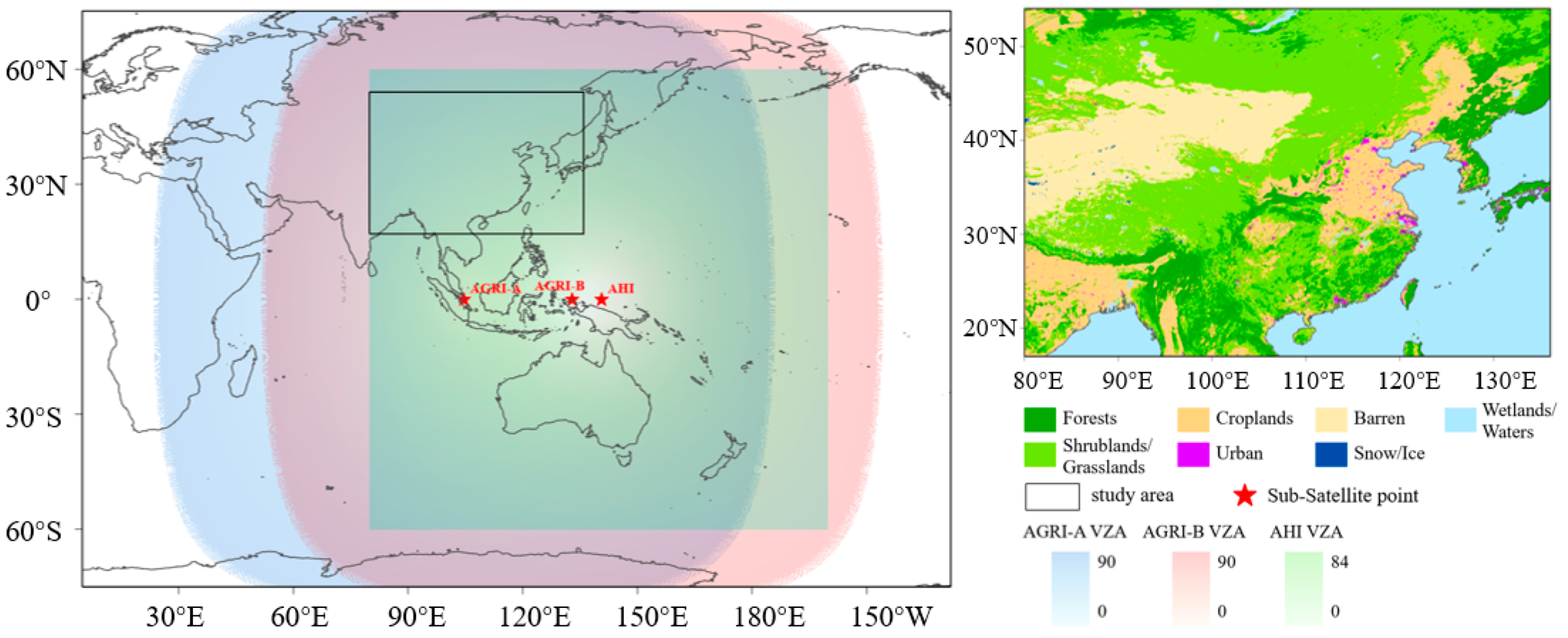
Figure 1. Geostationary orbit satellite observation range and study area.
Remotesensing 17 03315 g001
Figure 2. The frameworks of TCM, MCM, and CCM algorithms.
Remotesensing 17 03315 g002
Figure 3. Performance of TCM, MCM, and CCM algorithms under CALIOP validation.
Remotesensing 17 03315 g003
Figure 4. Performance of TCM, MCM, and CCM algorithms under MODIS validation.
Remotesensing 17 03315 g004
Figure 5. Comparison of MOD35/MOD35 with the TCM-CM of AGRI-A, AGRI-B, and AHI. (a) Case a; (b) Case b; (c) Case c; (d) Case d. (The first row of each case is TCM-CM, with colorless represents cloudy and blue represents clear. The second row shows the difference between the TCM-CM and MODIS cloud mask products. The third row shows the difference between the FY-4A CLM, FY-4B CLM, and H8/H9 CLP cloud products and the MODIS cloud mask products. Rosy color represents that MODIS is cloudy and the control is clear, green color represents that MODIS is clear and the control is cloudy, and colorless represents MODIS and the control have the same classification. The red boxes are the boundaries of the MODIS cloud products.).
Remotesensing 17 03315 g005aRemotesensing 17 03315 g005bRemotesensing 17 03315 g005c
Figure 6. Overall validation scores for MODIS cases.
Remotesensing 17 03315 g006
Figure 7. Comparison of TCM-CM of AGRI-A, AGRI-B, and AHI with CALIOP VFM and FY-4A CLM, FY-4B CLM, and H8/H9 CLP. (Colorless represents cloudy, blue represents clear. The red line represents that the CALIOP is cloudy, while the yellow line represents that the CALIOP is clear).
Remotesensing 17 03315 g007
Figure 8. Overall validation scores for CALIOP cases.
Remotesensing 17 03315 g008
Figure 9. SHAP summary plots of TCM models for AGRI-A, AGRI-B, and AHI. (a) TCM model for AGRI-A; (b) TCM model for AGRI-B; (c) TCM model for AHI. (The horizontal axis represents the SHAP value, while the vertical axis lists the features. A positive SHAP value indicates that the feature contributes to increasing the probability of a pixel being classified as cloudy, while a negative SHAP value indicates the opposite effect, favoring clear-sky classification. The color scale indicates the actual feature value, and the thickness of the plot reflects the density of samples).
Remotesensing 17 03315 g009aRemotesensing 17 03315 g009b
Figure 10. Variations in the matching counts and accuracies of the TCM-CM from AGRI-A, AGRI-B, and AHI across different ranges of SZA.
Remotesensing 17 03315 g010
Figure 11. Variations in the matching counts and accuracies of the TCM-CM from AGRI-A, AGRI-B, and AHI across different ranges of VZA.
Remotesensing 17 03315 g011
Figure 12. Variations in the matching counts and accuracies of the TCM-CM from AGRI-A, AGRI-B, and AHI across different IGBP.
Remotesensing 17 03315 g012
Figure 13. Comparison of cloud detection accuracy for TCM, MCM, and CCM across different IGBP surface types based on CALIPSO and MODIS validation. (a) CALIOP validation for AGRI-A CM; (b) CALIOP validation for AGRI-B CM; (c) CALIOP validation for AHI CM; (d) MODIS validation for AGRI-A CM; (e) MODIS validation for AGRI-B CM; (f) MODIS validation for AHI CM.
Remotesensing 17 03315 g013aRemotesensing 17 03315 g013b
Figure 14. Normalized mean SHAP values for TCM models of AGRI-A, AGRI-B, and AHI.
Remotesensing 17 03315 g014
Figure 15. RF Importance Score for TCM models of AGRI-A, AGRI-B, and AHI.
Remotesensing 17 03315 g015
Table 1. Detailed parameters of the sensors for this study.
SensorSatelliteShort NameSub-Satellite PointSpatial
Resolution
(km)
Temporal
Resolution
(min)
Scanning
Continuity
AGRIFY-4AAGRI-A105.0°E415incomplete continuity
FY-4BAGRI-B133.0°E415completely continuous
AHIH-8/H-9AHI140.7°E510completely continuous
Table 2. Specification of AGRI-A, AGRI-B and AHI.
RenameAGRI-AAGRI-BAHI
NoBand (μm)NoBand (μm)NoBand (μm)
B110.4710.4710.47
----20.51
B220.6520.6530.64
B330.8330.82540.86
41.3741.379--
B451.6151.6151.6
B562.2262.22562.3
B673.72 (high)73.75 (high)73.9
83.72 (low)83.75 (low)--
B796.2596.2586.2
--106.9596.9
B8107.10117.42107.3
B9118.50128.55118.6
----129.6
B101210.801310.801310.4
----1411.2
B111312.01412.01512.4
B121413.51513.31613.3
Table 3. IGBP land cover type names, values, and reclassification types.
IGBP Class NameIGBP Class ValueReclassification Types
Evergreen Needleleaf Forests1Forests
Evergreen Broadleaf Forests2Forests
Deciduous Needleleaf Forests3Forests
Deciduous Broadleaf Forests4Forests
Mixed Forests5Forests
Closed Shrublands6Shrublands/Grasslands
Open Shrublands7Shrublands/Grasslands
Woody Savannas8Shrublands/Grasslands
Savannas9Shrublands/Grasslands
Grasslands10Shrublands/Grasslands
Permanent Wetlands11Wetlands/Waters
Croplands12Croplands
Urban and Built-up Lands13Urban
Cropland/Natural Vegetation Mosaics14Croplands
Permanent Snow and Ice15Snow/Ice
Barren16Barren
Water Bodies17Wetlands/Waters
Table 4. Dichotomous confusion matrix.
Cloudy (Predicted Values)Clear (Predicted Values)
Cloudy (true values)ab
Clear (true values)cd
Table 5. CALIOP validation results.
SensorMatched Pixels P O D c l d P O D c l r F A R c l d F A R c l r HRKSS
AGRI-A11,2870.91280.84350.12500.11040.88130.7563
AGRI-B11,2870.91330.81970.14130.11270.87070.7330
AHI81390.93730.79330.09700.13950.89020.7307
Table 6. MODIS validation results.
SensorMatched Pixels ( × 108) P O D c l d P O D c l r F A R c l d F A R c l r HRKSS
AGRI-A2.190117560.90460. 79460.11760.16990.86390.6992
AGRI-B2.189148530.89980. 78420.12340.17880.85710.6840
AHI1.432437020.89560. 78610.12240.18520.85530.6817
Table 7. Validation scores for MODIS cases.
CaseValueAGRI-A CMFY-4A CLMAGRI-B CMFY-4B CLMAHI CMH8/H9 CLP
aHR0.83690.78790.82650.77060.80790.7542
P O D c l d 0.85410.88900.84550.90870.82930.9338
F A R c l d 0.13740.22340.14680.24430.16290.2776
bHR0.87530.85420.86710.85690.86860.8351
P O D c l d 0.64390.57280.60050.59710.60870.6485
F A R c l d 0.13500.15690.12660.16820.12820.2798
cHR0.87710.79040.87670.80390.88030.7410
P O D c l d 0.85770.65840.85950.72090.86930.7442
F A R c l d 0.09490.07640.09720.11260.09900.2389
dHR0.90220.86360.89770.87290.89230.8718
P O D c l d 0.94580.93780.94550.95400.94240.9053
F A R c l d 0.07310.11120.07810.11240.08200.0755
Mean (all cases)HR0.87110.82130.86530.82330.86110.7950
P O D c l d 0.84860.78730.84000.81930.83860.8276
F A R c l d 0.10580.14780.10950.16730.11610.2161
Table 8. Validation scores for CALIOP cases.
CaseValueAGRI-AFY-4A CLMAGRI-BFY-4B CLMAHIH8/H9 CLP
eHR0.91510.82700.91190.82390.89850.7331
P O D c l d 0.98221.00000.98220.98821.00001.0000
F A R c l d 0.12630.24550.13090.24430.16170.3365
fHR0.84550.80730.82060.76250.80900.7639
P O D c l d 0.90710.90980.91530.93720.94370.9683
F A R c l d 0.15090.19950.81310.25920.22320.2782
gHR0.93020.83570.91380.87060.87300.8307
P O D c l d 0.97040.89780.96510.93550.92550.9184
F A R c l d 0.05990.11170.07470.10080.09380.1367
Mean (all cases)HR0.89050.82160.87350.81380.85150.7790
P O D c l d 0.94710.92170.94820.94600.94760.9547
F A R c l d 0.10980.17720.13220.19890.16370.2444
Table 9. Normalized mean SHAP values for TCM models of AGRI-A, AGRI-B, and AHI.
ModelB1B2B3B4B5B6B7B8B9B10B11B12SZAVZARAA
TCM for ARGI-A9.043.583.012.823.654.723.687.456.297.1922.894.3410.137.064.15
TCM for AGRI-B12.804.603.593.364.034.514.065.523.177.1815.956.489.6810.834.35
TCM for AHI10.486.342.633.364.295.182.172.913.779.2028.873.654.928.943.31
Disclaimer/Publisher’s Note: The statements, opinions and data contained in all publications are solely those of the individual author(s) and contributor(s) and not of MDPI and/or the editor(s). MDPI and/or the editor(s) disclaim responsibility for any injury to people or property resulting from any ideas, methods, instructions or products referred to in the content.