Article

Discrimination of Multiple Foliar Diseases in Wheat Using Novel Feature Selection and Machine Learning

National Engineering and Technology Center for Information Agriculture (NETCIA), MARA Key Laboratory for Crop System Analysis and Decision Making, MOE Engineering Research Center of Smart Agriculture, Jiangsu Key Laboratory for Information Agriculture, Nanjing Agricultural University, 1 Weigang Road, Nanjing 210095, China
*
Author to whom correspondence should be addressed.
These authors contributed equally to this work.
Remote Sens. 2025, 17(19), 3304; https://doi.org/10.3390/rs17193304
Submission received: 31 July 2025 / Revised: 11 September 2025 / Accepted: 18 September 2025 / Published: 26 September 2025

Abstract

Highlights

What are the main findings?
  • The CWPA-KNN combination achieved a high overall accuracy of 77% in dis-criminating wheat leaves infected with diseases, e.g., powdery mildew, stripe rust, leaf rust.
  • Only two key wavelet-based features (668 nm at scale 5 and 894 nm at scale 7) were needed for effective multi-disease differentiation, streamlining the detection process.
What is the implication of the main finding?
  • The study provided a systematic and efficient detection method, integrating fea-ture selection and machine learning, and offering direct technical support for pre-cise disease management in the field.
  • A comprehensive and severity-classified hyperspectral database was established for wheat foliar disease detection, providing a valuable resource for future re-search.

Abstract

Wheat, a globally vital food crop, faces severe threats from numerous foliar diseases, which often infect agricultural fields, significantly compromising yield and quality. Rapid and accurate identification of the specific disease is crucial for ensuring food security. Although progress has been made in wheat foliar disease detection using RGB imaging and spectroscopy, most prior studies have focused on identifying the presence of a single disease, without considering the need to operationalize such methods, and it will be necessary to differentiate between multiple diseases. In this study, we systematically investigate the differentiation of three wheat foliar diseases (e.g., powdery mildew, stripe rust, and leaf rust) and evaluate feature selection strategies and machine learning models for disease identification. Based on field experiments conducted from 2017 to 2024 employing artificial inoculation, we established a standardized hyperspectral database of wheat foliar diseases classified by disease severity. Four feature selection methods were employed to extract spectral features prior to classification: continuous wavelet projection algorithm (CWPA), continuous wavelet analysis (CWA), successive projections algorithm (SPA), and Relief-F. The selected features (which are derived by CWPA, CWA, SPA, and Relief-F algorithm) were then used as predictors for three disease-identification machine learning models: random forest (RF), k-nearest neighbors (KNN), and naïve Bayes (BAYES). Results showed that CWPA outperformed other feature selection methods. The combination of CWPA and KNN for discriminating disease-infected (powdery mildew, stripe rust, leaf rust) and healthy leaves by using only two key features (i.e., 668 nm at wavelet scale 5 and 894 nm at wavelet scale 7), achieved an overall accuracy (OA) of 77% and a map-level image classification efficacy (MICE) of 0.63. This combination of feature selection and machine learning model provides an efficient and precise procedure for discriminating between multiple foliar diseases in agricultural fields, thus offering technical support for precision agriculture.

1. Introduction

Wheat is a critical food crop for ensuring a stable global food supply [1]. However, global climate change and increasingly complex growing environments have led to a rise in the incidence of wheat foliar diseases, such as powdery mildew, stripe rust, and leaf rust [2,3]. These diseases impair photosynthetic efficiency, threatening both yield and grain quality [4,5]. Thus, developing efficient techniques for discrimination between multiple diseases is a critical requirement for precision disease management, targeted pesticide application, and sustainable agriculture.
Currently, plant disease identification primarily relies on RGB image classification technology, which analyzes visible phenotypic characteristics of diseases (e.g., color, texture, and lesion morphology) and has achieved high accuracy in diagnosing crop diseases [6,7,8]. However, this approach depends on large-scale annotated datasets and incurs high computational costs. Moreover, it can only identify diseases at symptomatic stages, making early warning and large-scale rapid monitoring challenging [9,10]. In contrast, remote sensing spectroscopy captures the spectral responses of crops across multiple bands (e.g., visible and near-infrared), reflecting internal physiological and biochemical changes (e.g., chlorophyll degradation and water loss) [11,12,13]. This enables efficient and precise identification of latent infection through advanced symptomatic stages. For instance, Yuan et al. [14] achieved high-accuracy discrimination between healthy and diseased tea leaves using hyperspectral data, with an overall accuracy (OA) of 0.98 and a kappa coefficient of 0.94; Tian et al. [15] successfully identified different infection stages of rice blast using hyperspectral data, achieving a classification accuracy exceeding 95%. However, hyperspectral data are characterized by high dimensionality, strong inter-band collinearity, and potential similarity in spectral responses across different diseases, which can lead to feature redundancy and reduced model generalizability [16]. Therefore, effective feature selection is a critical prerequisite for extracting discriminative information from massive spectral data and building robust classification models.
Existing studies have successfully achieved high accuracy in identifying single diseases using relevant feature selection methods [17,18]. For example, Sun et al. [19] used SPA to select three optimal wavelengths (617 nm, 675 nm, and 818 nm) to construct a classification model for peach decay, achieving 98.75% accuracy; Cheng et al. [20] applied CWA to identify spectral features correlated with tree health, enabling early detection of “green attack” damage caused by mountain pine beetle. However, real-world field often involves the coexistence of multiple diseases, where their spectral features interfere with each other, imposing higher demands on the robustness of feature selection. At present, there remains a lack of systematic comparison and evaluation of different feature selection algorithms in complex multi-disease identification scenarios, and it is still unclear which method can optimally extract sensitive features common to multiple diseases [21]. Furthermore, most current studies rely on spectral data collected under specific experimental conditions, within a single year, or during particular growth stages [22,23]. There is a notable scarcity of spectral databases that cover multiple disease types, diverse growing conditions, and spatiotemporal variations [24]. This limitation results in insufficient generalization capability of existing methods in multi-disease scenarios, making it difficult to meet the complex demands of practical agricultural disease monitoring. Therefore, developing effective feature selection algorithms capable of extracting highly discriminative features and constructing disease recognition models with strong generalization capabilities has become a core technical challenge in addressing multi-disease identification
Recently, machine learning has been widely adopted for crop disease identification due to its computational efficiency and classification accuracy [25,26]. For instance, Huang et al. [27] developed a disease discrimination model that used selected spectral bands, vegetation indices, and wavelet features from winter wheat canopy hyperspectral data, which were classified with Fisher linear discriminant analysis (FLDA) and support vector machines (SVMs). Their model achieved classification accuracies of, respectively, 78.1% and 95.6% for powdery mildew and stripe rust. So, Li et al. [28] further developed a monitoring framework coupling K-nearest neighbors (KNN) with logistic regression, integrating remote sensing and meteorological factors (including average temperature, humidity and precipitation) for high-accuracy wheat Fusarium head blight detection; Anand et al. [29] demonstrated that the combination of hyperspectral data with decision tree (DT) and SVM algorithms enabled real-time detection of leaf spot disease in eggplant with a classification accuracy of 88%. However, it is still insufficient for the exploration of hyperspectral-based multi-disease identification and effective classification models, leaving the application of machine learning in complex crop disease monitoring unclear.
To address these gaps, this study aims to transcend single-disease limitations by differentiating multiple diseases using field spectra of leaves and a combination of feature selection and machine learning. Specific objectives include:
(1)
Building a hyperspectral database of wheat foliar diseases: systematically collect hyperspectral data of wheat leaves from multi-year field trials, with plants affected by powdery mildew, stripe rust, and leaf rust, to build a spatiotemporally representative spectral library.
(2)
Extracting and selecting disease spectral features: compare multiple feature selection algorithms (SPA, CWA, CWPA, and Relief-F) to identify disease-related spectral features and reduce redundancy.
(3)
Building high-accuracy disease identification models: compare the machine learning algorithms of KNN, naive Bayes (NB), and random forest (RF) for the construction of classification models using the features selected under objective (2).
(4)
Evaluating the accuracy of models: test the performance of various algorithms against their classification accuracy and model stability, to provide scientific and technical insight regarding efficient disease monitoring.

2. Materials and Methods

2.1. Experimental Design

This study comprises three wheat inoculation experiments (Experiments 1–3, conducted in 2018–2019 and 2022–2024) and one field experiment in a natural powdery mildew epidemic area (Experiment 4, 2023–2024). The individual experiments are described below (see Table 1):
Experiment 1: Pot-based powdery mildew trial
This experiment was conducted in 2017–2018 at the Pailou Teaching and Research Base of Nanjing Agricultural University (118°15′E, 32°1′N), Weigang District, Nanjing, Jiangsu Province, and employed a pot-culture design. Two cultivars were tested: the powdery mildew-susceptible wheat variety “Nannong 0686,” and the resistant variety “Nannong 9918” carrying disease-resistant genes. Pots (28 cm diameter) were filled with a 1:1:1 mixture of raw soil, vermiculite, and a nutrient-rich substrate. Each variety was planted in 24 pots, of which eight served as the control, and the remaining 16 were inoculated with powdery mildew spores at the jointing and booting stages (eight pots per stage). Post-inoculation, the groups were maintained in separate greenhouses under uniform management to prevent cross-contamination. The experimental data were collected at three principal growth phases: jointing, booting, and heading stages.
Experiment 2: Field trials for stripe rust and leaf rust
Experiment 2 was conducted in 2022–2023 at the Baima Experimental Station (119.18°E, 31.61°N), Lishui District, Nanjing, Jiangsu Province. Three cultivars were grown: the highly susceptible “Nannong 0686”, the moderately susceptible “Yangfumai 8161”, and the highly resistant “Nannong 92R137”. Each variety was planted in a total of nine plots (1.5 m × 4 m) comprising three control plots and six plots that were inoculated at the jointing stage (three plots for stripe rust and three for leaf rust). Fertilization followed local high-yield practice: total N (225 kg·ha−1), K2O (135 kg·ha−1), and P2O5 (120 kg·ha−1), with nitrogen split equally between basal (50%) and jointing-stage (50%) applications. The experimental data were collected at three principal growth phases: jointing, booting, and heading stages.
Experiment 3: Replicated field trial for stripe rust and leaf rust
This experiment was conducted in 2023–2024 at the same site as Experiment 2, with an identical experimental design.
Experiment 4: Field trial in a natural powdery mildew epidemic area.
Experiment 4 was carried out on 25 April 2024, at the Baima Experimental Station in a naturally powdery mildew-infected wheat field (25 m × 30 m) during the heading stage. The susceptible variety “Nannong 0686” was used, with sowing dates, cultivation practices (e.g., spacing, fertilization), and management aligned with local high-yield protocols. Only infected leaf samples were collected.

2.2. Data Acquisition

2.2.1. Hyperspectral Data Acquisition

The leaf hyperspectral data were collected non-destructively using a FieldSpec 4 high-resolution spectroradiometer (Analytical Spectral Devices, Boulder, CO, USA) equipped with a leaf clip, which was attached directly to the intact leaves during measurement. Each measurement was completed within two minutes. The spectrometer acquires data over the spectral range of 350–2500 nm. The spectrometer’s leaf clip attachment features an integrated active light source in a controlled, enclosed environment, and it produces generally stable measurements, with minimal noise. To ensure representative sampling, leaves from different vertical positions (e.g., D1, D2, and D3, where D1 represents the topmost fully expanded leaf) with health status and varying severity levels were selected. For each leaf, spectral measurements were taken at three positions (1/3, 1/2, and 2/3 of the distance from the leaf base to the leaf tip), with the leaf clip carefully positioned to avoid major veins and minimize measurement errors (Figure 1). The average reflectance of the three measurements was used as the final spectrum for each leaf sample.

2.2.2. Disease Typing and Severity Assessment

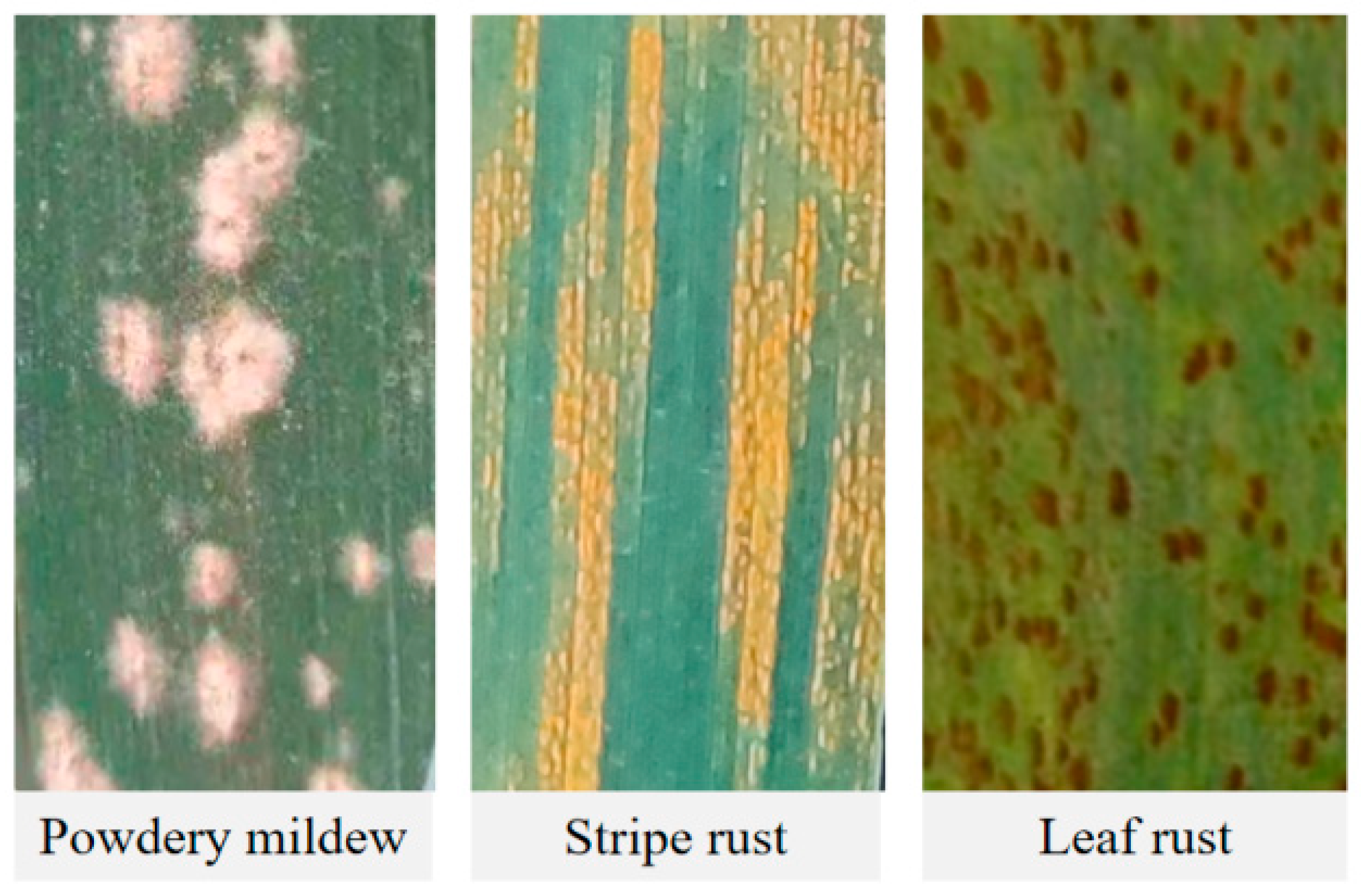
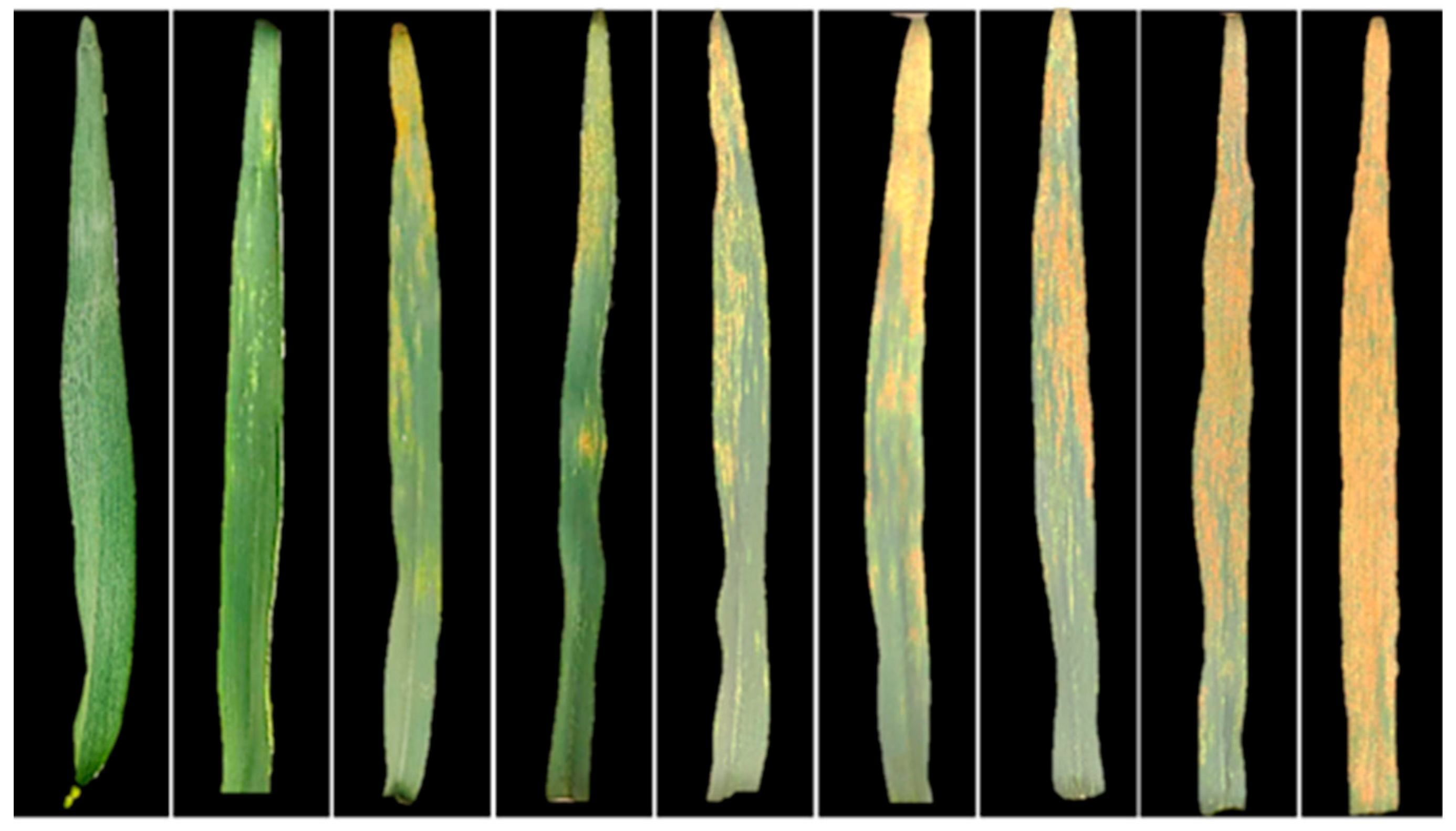
At the same time as the collection of hyperspectral measurements, corresponding agronomic parameters were acquired, including disease type, severity level, and leaf chlorophyll content. Disease typing and severity assessment were conducted by a specialist, strictly following the detailed guidelines and visual scales specified in the Chinese national standards for wheat disease evaluation (NY/T 613-2002 [30] for powdery mildew, NY/T 617-2002 [31] for leaf rust, and GB/T 15795-2011 [32] for stripe rust). For each infected leaf, the lesion type and the percentage of lesion area relative to total leaf area were systematically recorded. Based on lesion characteristics (Figure 2) and coverage percentage, disease severity was classified into one of eight progressive levels: 1%, 5%, 10%, 20%, 40%, 60%, 80%, and 100% (Figure 3).
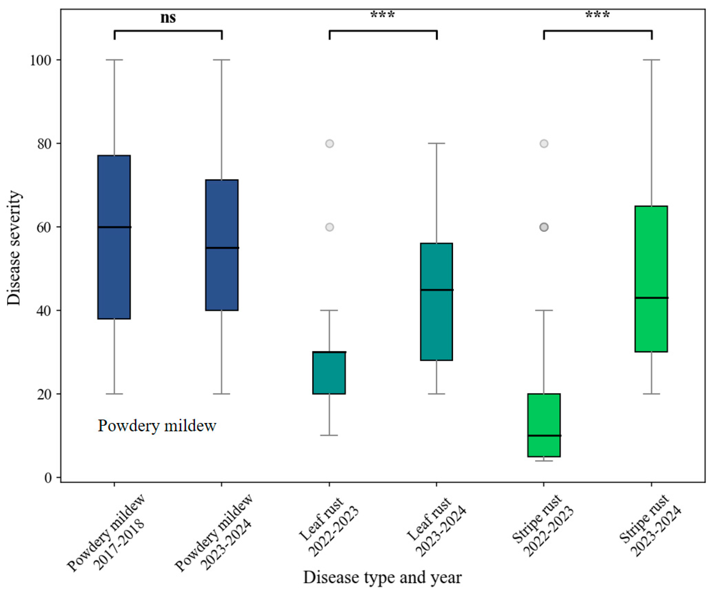
The distribution of disease severity data across different years for each disease is shown in Figure 4. It reveals no significant differences in the severity distribution of powdery mildew across years, indicating that the data for this disease are representative in all years. In contrast, significant inter-annual variations are observed in the severity distributions of stripe rust and leaf rust. Therefore, the training and validation datasets are divided according to interannual differences as described in Section 2.5.

2.2.3. Leaf Chlorophyll Data

At the same time as the collection of hyperspectral measurements, corresponding agronomic parameters were acquired, including leaf chlorophyll content, disease type, and severity level. Among them, leaf chlorophyll content is a key indicator of a plant’s photosynthetic capacity and overall health. It plays a particularly significant role in characterizing physiological and biochemical responses to disease stress in wheat. A primary manifestation is the degradation of chlorophyll in infected areas. The pattern and extent of chlorophyll loss can vary significantly depending on the pathogen type (e.g., fungal, bacterial, viral), thereby providing crucial biochemical evidence to distinguish between different disease types and their specific infection mechanisms. Leaf chlorophyll content was measured using a portable Dualex® leaf meter (Force-A, Orsay, France). For each leaf, three measurements were taken at positions corresponding to 1/3, 1/2, and 2/3 of the distance from the leaf base to the leaf tip, and the average value was used as the representative chlorophyll content for the leaf.

2.3. Common Feature Extraction Algorithms for Disease Identification

This study implemented a two-stage algorithmic framework of “feature extraction + classification”. In the first stage, four advanced feature extraction methods were employed to identify the most discriminative features from high-dimensional spectral data: CWA, SPA, CWPA, and Relief-F. In the second stage, the optimized feature subsets were input into machine learning classification models to enhance computational efficiency and improve generalization capability, with the aim of achieving precise disease identification. All model development and data analysis were implemented in MATLAB R2023a (MathWorks Inc., Natick, MA, USA).

2.3.1. Continuous Wavelet Analysis (CWA)

CWA is a spectral processing method that decomposes reflectance spectra across continuous scales and wavelengths using a continuous wavelet transform to generate a wavelet coefficient matrix [7,8]. Following decomposition, wavelet coefficients sensitive to target parameters are extracted to construct wavelet feature sets. Compared to conventional spectral indices, wavelet features not only characterize spectral intensity information but also capture critical spectral shape characteristics. These features can be employed individually to represent spectral shapes at specific bands or combined to simultaneously reflect both global spectral trends and local details, thereby enhancing target signals while suppressing background interference. Consequently, multi-scale wavelet features enable the extraction of both global spectral variation patterns and localized subtle fluctuations. The mathematical expression for CWA’s decomposition of original spectra using wavelet basis functions is as follows [33]:
Ψ a , b λ = 1 a Ψ λ b a
where a is the scaling factor, and b is the shifting factor. Ψ a , b λ represents the wavelet basis functions ( λ = 1, 2, …, n, with n being the number of spectral bands). The original spectrum is decomposed into wavelet coefficients after a continuous wavelet transform. The expression of the wavelet coefficients is as follows [33]:
W f a , b = f , Ψ a , b = + f λ Ψ a , b λ d λ
where f λ represents the reflectance spectrum ( λ = 1, 2, …, n, with n being the number of spectral bands). The wavelet coefficients W f a i , b j (i = 1, 2, …, m; j = 1, 2, …, n) form a two-dimensional wavelet coefficient map (an m × n matrix), where m represents the number of decomposition scales [26]. Considering that vegetation spectral absorption features typically exhibit quasi-Gaussian characteristics, we adopted a quasi-Gaussian function as the wavelet basis. The decomposition scales were set as 2i (i = 0, 1, 2,…, 7) to reduce computational complexity [20,34].
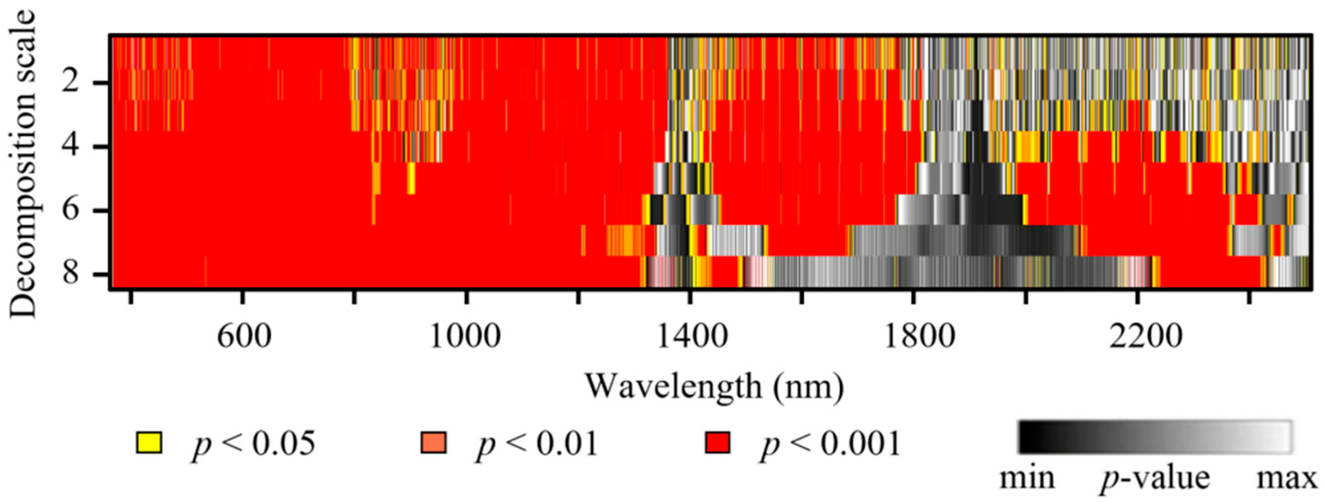
The continuous wavelet decomposition generated corresponding wavelet coefficients at the specified scales for each input spectral curve. We performed analysis of variance (ANOVA) on the wavelet coefficients across the three stress conditions for each band and scale, ultimately obtaining a 2151 (spectral bands) × 8 (decomposition scales) p-value matrix (wavelet sensitivity coefficient map). This matrix quantifies the discriminative capability of the wavelet coefficients among the three stress conditions at each spectral band and scale, where smaller p-values indicate stronger differentiating power (higher sensitivity). The wavelet sensitivity coefficient map is therefore used to guide feature selection [7]. Based on the ranked p-values, we retained the most sensitive wavelet coefficient regions (corresponding to the smallest p-values) at 1%, 5% and 10% thresholds. Using an 8-neighborhood criterion, we then identified independent connected domains and extracted the most sensitive wavelet coefficient within each domain to form the final wavelet feature set [33].

2.3.2. Successive Projection Algorithm (SPA)

SPA is a forward feature selection algorithm that minimizes collinearity in vector space by selecting feature combinations with minimal information redundancy through projection operations between feature vectors [35]. The algorithm initiates from a starting spectral band x 1 . During each iteration, it computes the projections of the remaining spectral bands onto the subspace orthogonal to x 1 . The wavelength exhibiting the maximum projection vector is then incorporated into the feature set, ensuring the least possible correlation between successively selected bands. This iterative process continues for n cycles to obtain an optimal combination of spectral bands with the specified number of features. If the initial band x 1 and iteration number n are not specified, the algorithm can exhaustively evaluate all possible spectral bands to generate candidate feature sets. The optimal feature combination is subsequently determined by assessing classification model performance, using accuracy metrics as feedback. The feature selection process in this study applied this approach. Detailed implementation procedures can be found in Araújo et al. [36].

2.3.3. Continuous Wavelet Projection Algorithm (CWPA)

Both CWA and SPA have been widely used as classical spectral feature extraction and selection algorithms for plant monitoring [7,35], yet these methods exhibit limitations in, respectively, feature combination optimization and information mining depth [33]. An ideal spectral feature set should demonstrate high sensitivity to target parameters while maintaining low redundancy. CWPA attempts to achieve this ideal by integrating CWA’s spectral information extraction capability with SPA’s feature optimization capacity [33]. The algorithm is implemented as follows:
Step 1: Perform a continuous wavelet transformation on the original spectral library (s samples × b bands) to generate wavelet coefficient matrices (W1, W2 … Wn) across n decomposition scales, forming a three-dimensional wavelet feature matrix (s samples × b bands × n scales).
Step 2: Transform the 3D wavelet feature matrix into a 2D matrix WF (s samples × (b bands × n scales)) to integrate band and scale information.
Step 3: Apply successive projections to WF under specified feature numbers to generate b × n feature combinations.
Step 4: Conduct analysis of variance (ANOVA) for each feature combination and calculate the corresponding mean p-value. The feature combination associated with the minimum p-value is selected as the optimal combination for that feature number.
Step 5: Iterate Steps 2–4 across a predefined feature number range (1 − m) to obtain optimal feature combinations F1, F2 … Fm for each specified feature number.
Step 6: Input the m optimal feature combinations into classification or regression models and identify the final optimal feature combination corresponding to the maximum overall accuracy (OA).
Notably, unlike conventional wrapper-based feature selection methods, Step 4 initially filters different feature combinations of equal length based on statistical p-values, greatly reducing algorithmic complexity and computational time.

2.3.4. Relief-F Algorithm

The Relief-F algorithm is a classical feature selection method designed to identify features that contribute to classification tasks by evaluating their relevance to class labels [37]. This distance-based algorithm operates by randomly selecting a sample and adjusting feature importance weights according to its nearest neighbors from both the same class (nearest hits) and different classes (nearest misses). A key advantage of Relief-F lies in its distribution-free nature, requiring no assumptions about data distribution patterns while maintaining a strong capability to capture nonlinear relationships [38]. These characteristics have led to its widespread application in machine learning feature selection [39]. The feature selection process involved iteratively adding the most significant wavelengths until peak classification accuracy was attained

2.4. Disease Classification Model

The disease-sensitive feature sets produced by the four feature selection algorithms (CWA, SPA, CWPA, and Relief-F) were input into three different machine learning algorithms to evaluate the performance of the feature selection methods. We selected RF, KNN, and BAYES as classification models.

2.4.1. Random Forest Algorithm (RF)

RF is a machine learning method based on the ensemble of decision trees, which constructs multiple independent classification trees and employs a voting mechanism to generate the final prediction [40]. The algorithm first creates diverse training subsets through bootstrap sampling, then randomly selects feature subsets at each node split for optimal partitioning. Compared to a single decision tree model, RF effectively reduces model variance and enhances classification confidence [41]. In this study, a grid search approach was adopted to optimize key RF parameters (number of decision trees, maximum depth, and minimum leaf samples), with the overall classification accuracy of the validation set serving as the optimization objective.

2.4.2. K-Nearest Neighbors Algorithm (KNN)

The KNN algorithm is an instance-based, non-parametric classification method that determines class labels by analyzing proximity relationships in feature space [42]. KNN identifies the k closest neighbors of a test sample in the training set and assigns a class label via majority or weighted voting. This approach adapts well to complex nonlinear decision boundaries while preserving the local structural information of raw data. In this study, the optimal number of neighbors (k ∈ [1, 15]) was determined through empirical search, with Euclidean distance as the metric and uniform weighting for voting. The validation set’s overall classification accuracy was used as the optimization criterion.

2.4.3. Naïve Bayes Algorithm (BAYES)

BAYES, a probabilistic classifier based on Bayes’ theorem, constructs classification models by estimating conditional probabilities between features and classes [43]. Unlike deterministic classifiers, BAYES first estimates prior probability distributions for each class, then computes posterior probabilities by incorporating feature likelihoods, and finally assigns class labels based on maximum a posteriori (MAP) principles. This probabilistic framework captures global statistical relationships between features and classes by integrating prior knowledge with observed data. The optimization of BAYES’s smoothing parameter was conducted through empirical search, with validation set accuracy as the optimization target.

2.5. Data Analysis

In this study, the data from 2023 to 2024 exhibited the largest sample size and the most representative severity profiles, rendering them most suitable for model training. Accordingly, this study utilized the 2023–2024 data as the training set (n = 656), while data from other years were reserved as the validation set (n = 420) to evaluate the model’s cross-year transferability. The dataset partitioning scheme is presented in Table 1.

2.6. Model Evaluation Metrics

Disease classification model performance was assessed using two metrics: overall accuracy (OA) and map-level image classification efficacy (MICE). As a simplified version of the kappa coefficient, MICE eliminates the computation of reference category uncertainty [44]. The mathematical formulations for OA and MICE are provided in Equations (3) and (4).
O A = j = 1 J n j j n
M I C E = O A j = 1 J n j n 2 1 j = 1 J n j n 2
where n denotes the total sample size, n j j is the number of samples correctly classified as class j, and J is the total number of classes. n j is the reference total number as class j.

3. Results

3.1. Wheat Foliar Disease Identification Based on CWA and Machine Learning Models

Wavelet features extracted through CWA demonstrated strong overall sensitivity (Figure 5). Over 50% of the wavelet features exhibited significant discriminative power for wheat disease identification, meeting the criterion of p < 0.001. These sensitive wavelet features are found in four broad spectral regions: visible (400–750 nm), near-infrared (950–1300 nm), and shortwave infrared (1400–1800 nm and 2000–2400 nm). The wavelength range of sensitive features broadened with increasing decomposition scale. The most sensitive wavelet coefficients (corresponding to the smallest p-values) were selected at three thresholds corresponding to the highest 1%, 5%, and 10% sensitivity. Within each of these three datasets, independent connected domains were identified using an 8-neighborhood search. The most sensitive coefficient within each domain was selected to form the final wavelet feature set, yielding 29, 33, and 50 features for the three datasets, respectively. The specific wavelengths and associated scales for these selected features are listed in Table 2. Among the tested feature sets, the top 1% sensitivity threshold data achieved the highest classification accuracy (Figure 6), with overall accuracy (OA) values of 69% (RF), 71% (KNN), and 70% (BAYES), and MICE of 0.53 (RF), 0.54 (KNN), and 0.52 (BAYES).

3.2. Wheat Foliar Disease Identification Based on SPA and Machine Learning Models

The combination of SPA feature selection with the three machine learning methods resulted in a classification accuracy that generally increased as the number of selected features increased, until the accuracy reached a plateau, although the pattern shows considerable fluctuations (Figure 7). For the RF classifier, the highest classification accuracy was achieved with 38 features, yielding an OA of 59.5% and a MICE of 0.40 (Table 3). The KNN algorithm attained its peak performance with 32 features, achieving an OA of 69% and a MICE of 0.51. Similarly, the BAYES classifier reached its optimal accuracy with 35 features, resulting in an OA of 67% and a MICE of 0.50 (Table 3).

3.3. Wheat Foliar Disease Identification Based on CWPA and Machine Learning Models

Compared with CWA and SPA, CWPA not only considers feature sensitivity but also incorporates mutual information between features, generating an optimal feature subset by minimizing inter-feature redundancy (see Section 2.3.3 for details). Using only two features (668 nm, scale 5; 894 nm, scale 7), CWPA achieved high overall classification accuracies: 74% for RF, 77% for KNN, and 76% for BAYES (Figure 8 and Table 4). Notably, the CWPA model rapidly reached its peak accuracy before sharply declining, after which the accuracy fluctuated and slowly increased with additional features. However, the subsequent accuracy never surpassed the initial peak achieved with fewer features (Figure 8).

3.4. Wheat Foliar Disease Identification Based on Relief-F and Machine Learning Models

The classification accuracy of Relief-F combined with machine learning models exhibited a gradual upward trend as the number of features increased. RF, KNN, and BAYES reached their highest accuracies at 45, 39, and 25 features, respectively, with corresponding OAs of 0.49, 0.50, and 0.43, and MICE of 0.23, 0.21, and 0.16 (Figure 9 and Table 5). After reaching peak classification accuracy, performance declined, presumably due to the inclusion of redundant information (Figure 9). This suggests that while Relief-F can effectively extract some important features, increasing the number of features further does not substantially improve model accuracy. More importantly, the classification accuracy of these models was notably lower than that of CWPA combined with machine learning.

3.5. Summary

Four spectral feature selection algorithms (including CWA, SPA, CWPA, and Relief-F) were evaluated in combination with three machine learning classifiers (RF, KNN, and Bayes) for multiple wheat foliar disease identification. Notable performance disparities were observed among different algorithm-classifier combinations (Table 6). While CWA demonstrated relatively robust performance (OA = 69–71%), it required the selection of up to 29 spectral features (Table 6). SPA achieved moderate classification accuracy (OA = 59–69%) but needed 32–38 features (Table 6). Relief-F showed the weakest performance (OA = 43–50%) with 25–42 features (Table 6). In contrast, the CWPA achieved superior performance with minimal feature requirements (Table 6). When combined with the KNN classifier, the model achieved peak classification accuracy (OA = 77%, MICE = 0.63), suggesting this approach offers an optimal balance between feature parsimony and classification accuracy for wheat disease detection.

4. Discussion

4.1. Challenges in Accurate Identification of Multiple Wheat Foliar Diseases

Accurate identification of multiple wheat foliar diseases remains a critical scientific challenge in agricultural remote sensing. Most current studies primarily focus on binary classification between healthy and diseased foliar or single-disease detection [45,46]. These approaches mainly rely on monitoring physiological and biochemical changes, such as reduced chlorophyll content and decreased water content, combined with vegetation indices and spectral derivative transformations. Although these methods achieve classification accuracies of 85–95%, their performance in real-world agricultural production scenarios is generally not explored. Field investigations reveal that wheat is often simultaneously infected by multiple diseases, including yellow leaf spot, powdery mildew, stripe rust, and leaf rust (co-infection rates can exceed 35%). These diseases exhibit highly similar symptoms, such as chlorophyll degradation, water loss, and cellular structure damage, posing significant challenges for accurately identifying and distinguishing between multiple diseases [47]. However, subtle differences exist in lesion color and texture due to distinct pathogenic mechanisms. For example, powdery mildew forms white powdery spots on leaf surfaces, later turning grayish-brown [48]. Stripe rust produces bright yellow to orange-yellow lesions arranged in linear stripes (parallel to leaf veins) [49]. Leaf rust manifests as circular or irregular orange-red to reddish-brown lesions scattered across the leaf [50]. Previous studies suggest that these visible symptoms induce subtle spectral reflectance variations with disease-specific absorption features [47]. In this study, by coupling feature selection algorithms (CWA, SPA, CWPA, and Relief-F) with machine learning models (KNN, RF, and BAYES), we appear to have successfully captured these fine spectral differences, achieving accurate multi-disease identification with a maximum overall accuracy (OA) of 77% and an MICE of 0.63. In comparison with existing studies, such as the work by Yuan et al. [51] that achieved an overall accuracy (OA) of 75% and a kappa coefficient of 0.67 in classifying wheat stripe rust, powdery mildew, and aphids, and the study by Bebronne et al. [52], which reported an OA of 81% and a kappa of 0.6 for discriminating wheat stripe rust, leaf rust, and tan spot, the proposed method in this study accomplishes multiclass disease discrimination using only two key spectral features. It maintains competitive prediction accuracy while significantly enhancing feature utilization efficiency. However, a key limitation was observed during the early latent stage (DS < 20%), where underdeveloped lesions and indistinct symptoms led to substantially reduced identification accuracy. This represents a major constraint in current research and a critical direction for future breakthroughs.

4.2. Comparison of Advantages and Disadvantages Among Different Feature Selection Algorithms

Compared to the other feature selection algorithms, the widely used Relief-F method exhibited relatively low overall classification performance (e.g., maximum OA = 50%, MICE = 0.21 with KNN). For complex hyperspectral data, wavelength features may exhibit high collinearity and complex interactions. However, the Relief-F algorithm evaluates features based on their individual relevance to the target variable [37]. If two features are highly correlated and both are relevant to the labels, the Relief-F algorithm is likely to assign high weights to both. Since it does not account for inter-feature relationships, the resulting feature subset may contain a significant number of redundant features, rather than a compact, complementary set [38]. As shown in Table 5, the wavelengths selected by Relief-F are concentrated in the 350–400 nm region and fail to provide additional discriminative information to the classifier. Instead, they may introduce redundancy, which is likely the fundamental reason for its suboptimal performance. This phenomenon suggests that the Relief-F method is constrained by redundant information when processing hyperspectral data, limiting its applicability in high-dimensional data scenarios.
Instead, the CWPA method exhibited the best classification performance. Our results are consistent with those of Zhao et al. [33], who achieved an overall accuracy (OA) of up to 98% in tea disease classification using CWPA with only two key features. CWPA not only incorporates feature sensitivity but also generates an optimal feature combination by minimizing inter-feature redundancy. With only two features (668 nm at scale 5 and 894 nm at scale 7), CWPA achieved high classification accuracy (OA = 77%, MICE = 0.63 with KNN), notably outperforming the other algorithms. This indicates that CWPA can efficiently screen a small number of critical features, making it particularly suitable for hyperspectral data scenarios with high feature dimensionality. In contrast, the CWA method extracted features were found in four broad spectral regions (visible (400–750 nm), near-infrared (950–1300 nm), and shortwave infrared (1400–1800 nm and 2000–2400 nm)), encompassing multiple important bands related to disease response. However, apparently due to strong redundancy among features, its classification accuracy was limited (OA = 71%, MICE = 0.54 with KNN). The SPA method’s advantage lies in effectively reducing the number of features by eliminating redundant features through a successive projection algorithm, achieving relatively high classification performance within a specific range of feature numbers (e.g., OA = 69% with KNN using 32 features). However, its classification accuracy heavily depends on the number of features and model type, and its performance advantage is not as pronounced as that of CWPA. In summary, the CWPA method combines the dual advantages of sensitivity and redundancy control, enabling efficient disease classification with a small number of features. It is particularly suitable for rapid diagnosis tasks in precision agriculture disease monitoring.

4.3. Physiological Interpretation and Mechanistic Analysis of the Spectral Features Extracted by CWPA for Disease Identification

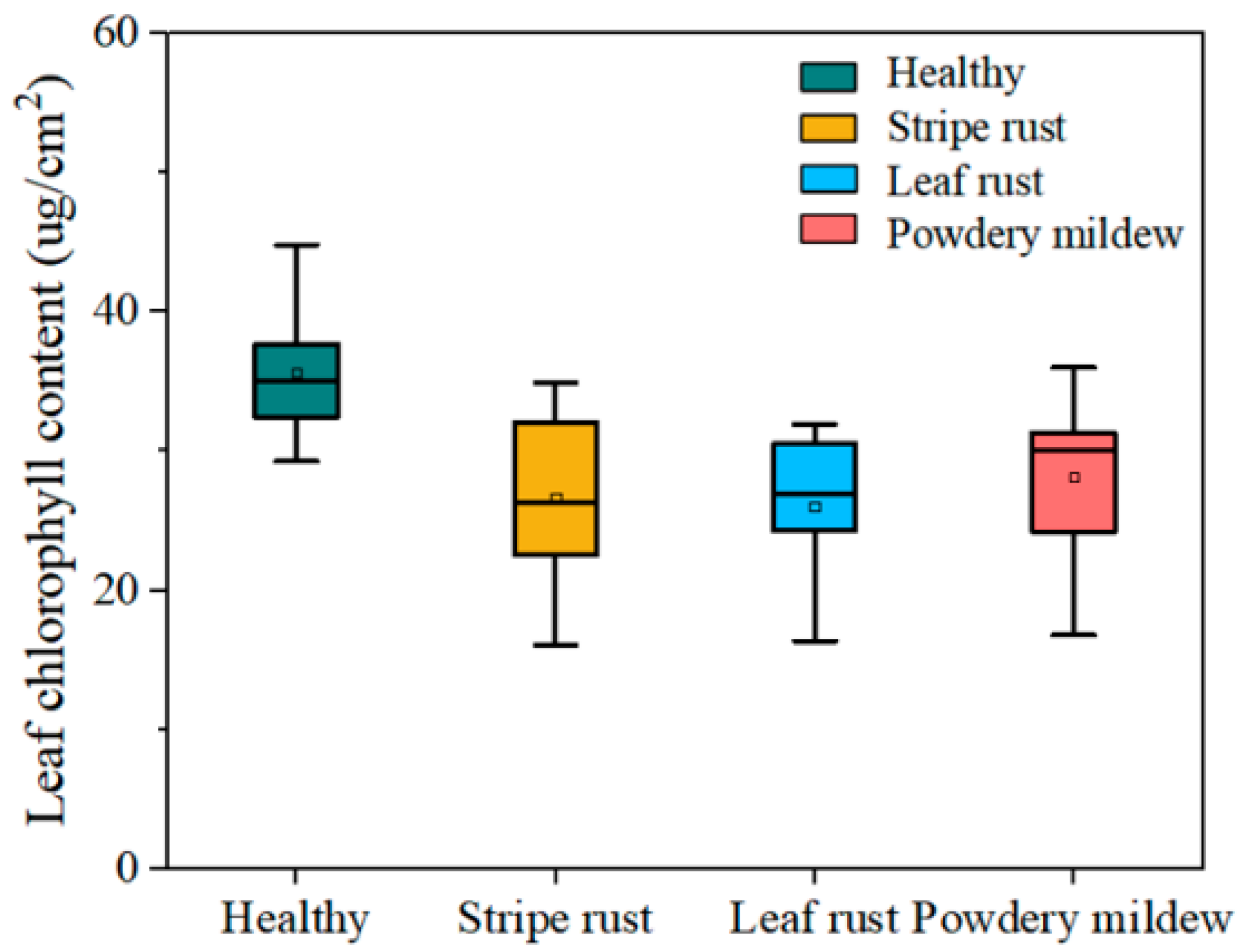
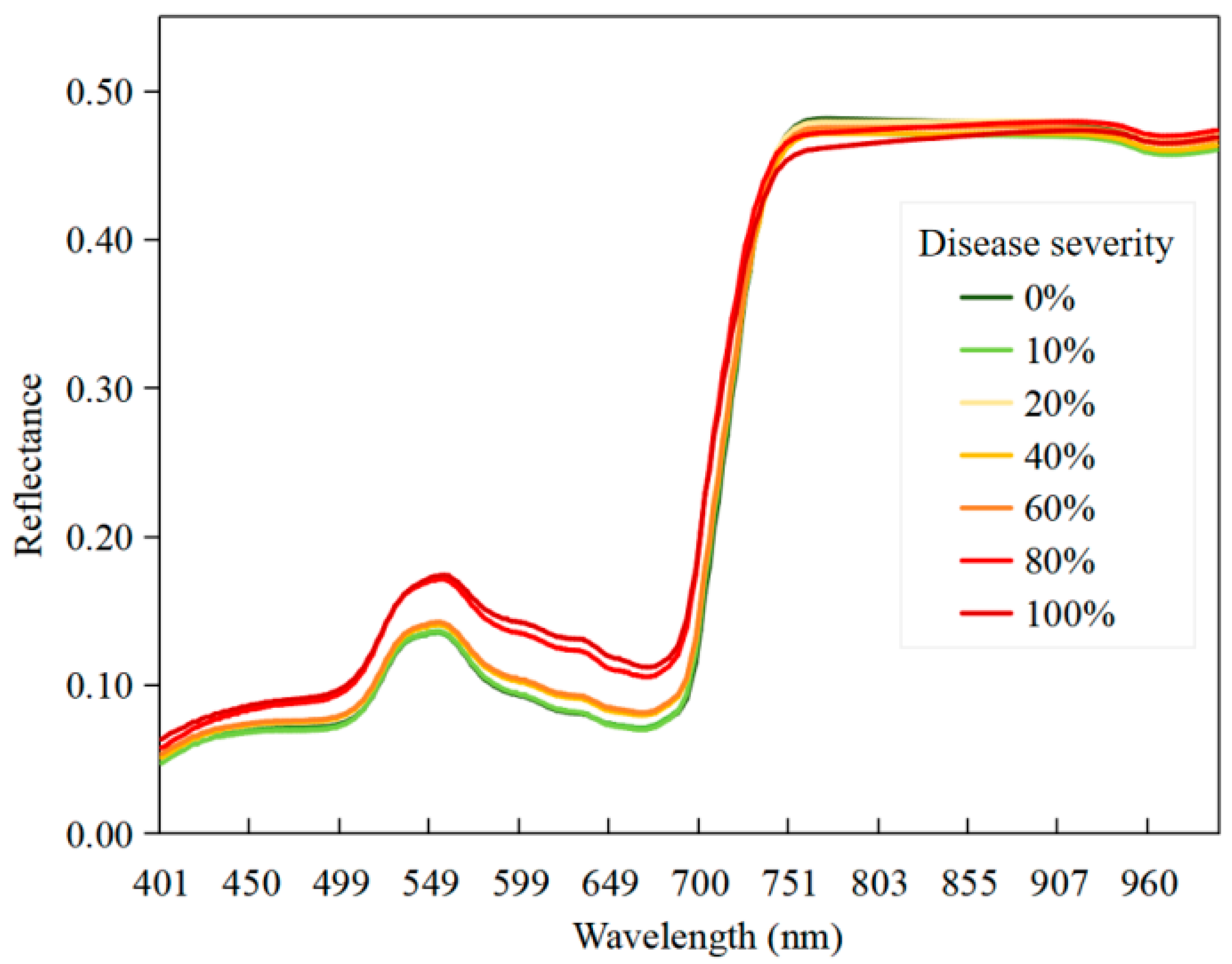
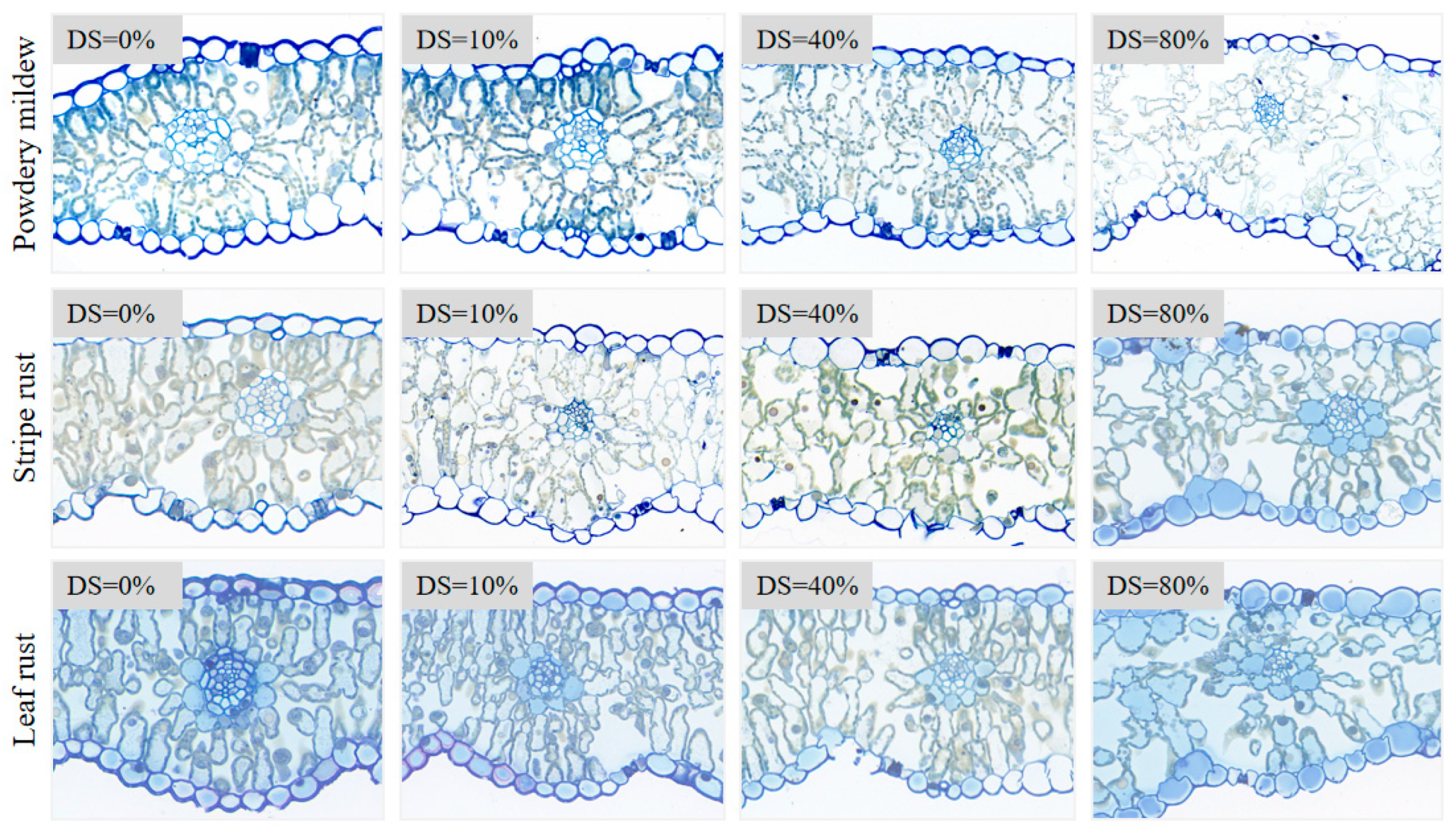
The superior performance of the CWPA in wheat disease classification stems from the correlation between its extracted spectral features and the physiological and biochemical responses to disease stress. Pathogen infection not only alters the appearance and structure of wheat leaves but also triggers a series of changes in physiological and biochemical processes [13]. First, disease infection leads to a reduction in photosynthetic pigments, such as chlorophyll, in lesion areas (Figure 10), resulting in a notable increase in reflectance within the visible spectrum (Figure 11). The 668 nm feature extracted by the CWPA at wavelet decomposition scale 5 is close to peak chlorophyll absorption in the red, and is thus sensitive to pigment metabolic imbalance [53]. This provides a stable spectral basis for disease identification. Furthermore, as pathogens invade, the structural integrity of leaf cell walls is compromised, and the arrangement of intercellular spaces is altered (Figure 12). These changes reduce light scattering in the red-edge to near-infrared (NIR) region, leading to a systematic decrease in reflectance (Figure 11). The 894 nm feature extracted at wavelet decomposition scale 7 exhibits a strong correlation with the degree of leaf anatomical structure degradation, and thus provides a measure of the extent of cellular damage [54,55]. Different pathogens causing powdery mildew, leaf rust, and stripe rust induce distinct pigment–structure coupled damage patterns. The selected dual-band features (668 nm and 894 nm) likely cover these two critical physiological responses. Additionally, the multi-scale nature of wavelet transforms further extracts hierarchical disease-related information. Thus, by coupling the 668 nm (pigment metabolism) and 894 nm (structural damage) features, the CWPA likely achieves synergistic monitoring of the dual physiological effects of disease. This approach not only minimizes redundant features but also enhances the accuracy and efficiency of classification models.

4.4. Advantages and Limitations of Coupling Feature Selection with Machine Learning and Its Potential for Early Disease Monitoring

Overall, the synergy between feature selection methods and machine learning models notably influenced classification performance, and the different machine learning algorithms exhibited differences in their sensitivity to the choice of feature selection method. Among the machine learning models, KNN demonstrated the highest overall classification accuracy. Regardless of the feature selection algorithm used, KNN achieved higher classification accuracy than RF and BAYES. For instance, with CWPA feature selection, KNN achieved the highest overall accuracy (OA = 77%, MICE = 0.63), outperforming RF (OA = 74%) and BAYES (OA = 76%). The superior performance of KNN may be attributed to its simple yet effective local neighborhood search mechanism [42], which efficiently utilizes the small number of highly sensitive features selected by CWPA. However, KNN’s performance heavily depends on the accuracy of feature selection. When redundant features were introduced (e.g., by Relief-F), their classification accuracy declined substantially (OA = 50%, MICE = 0.21). Similarly, the BAYES model exhibited notable performance variations under different feature selection strategies. For instance, when using CWA-selected 29 features, the BAYES model achieved its peak performance (OA = 70%). However, with a similar number of features (25) selected by Relief-F, its classification performance markedly declined (OA = 43%). This phenomenon may be related to the BAYES model’s dependence on the feature independence assumption [43]. When feature correlations exist (as in results from CWA and Relief-F), the model’s classification reliability may decrease. In contrast, the RF model showed minimal accuracy fluctuations (OA variation < 25%) when combined with different feature selection algorithms. In summary, the compatibility between feature selection algorithms and machine learning models is crucial. The combination of CWPA and KNN demonstrates superior classification performance in low-dimensional feature scenarios, making it the preferred choice for multiple foliar disease monitoring. Future research should further optimize feature selection algorithms to better align with different machine learning models, thereby enhancing classification performance and providing more efficient technical solutions for agricultural remote sensing applications.
Challenges still remain for foliar disease detection, particularly in the presence of other diseases and co-infections caused by multiple pathogens. The model was trained based on the specific diseases (including powdery mildew, stripe rust, leaf rust, and healthy leaves) (Table 1 and Table 6); it may not reliably detect or differentiate other foliar diseases not included in this study, such as leaf spot or downy mildew. Furthermore, the model may produce incorrect diagnoses in cases where leaves are co-infected by multiple pathogens, owing to the underrepresentation of such complex samples in the training dataset. Future research could further advance this work by combining mechanistic models with deep learning algorithms. Specifically, mechanistic models can simulate the effects of disease stress on plant physiological traits to generate extensive hyperspectral training data for deep learning models [56,57]. Deep learning algorithms can autonomously extract multi-dimensional features from large datasets, overcoming the dependency on feature selection inherent in traditional methods [58]. That will provide more efficient, accurate, and intelligent solutions for agricultural disease monitoring, thereby making greater contributions to global food security and sustainable agricultural development.

5. Conclusions

This study aimed to identify optimal feature-classifier combinations for discriminating multiple wheat foliar diseases using hyperspectral data. The comparative analysis revealed that the CWPA model, coupled with KNN, formed the most effective model. The main conclusions are as follows:
(1)
The CWPA demonstrated optimal performance in selecting common sensitive features for multiple wheat foliar diseases. CWPA not only effectively extracted sensitive features but also minimized inter-feature redundancy, showing notable advantages in balancing classification accuracy and feature quantity.
(2)
The optimal features selected by CWPA were two spectral bands at 668 nm and 894 nm, which, respectively, reflect the spectral response characteristics of pigment dynamics in wheat leaves under disease stress and cellular structure damage.
(3)
The CWPA–KNN algorithm developed in this study achieved high-accuracy identification of infected wheat leaves (OA = 77%, MICE = 0.63) using only two spectral features, greatly outperforming other algorithms such as RF and BAYES. This demonstrates the potential of this streamlined approach for efficient and accurate disease monitoring.

Author Contributions

Conceptualization, S.Z., Y.H. and J.Z.; Methodology, S.Z.; Software, Q.Y.; Formal analysis, Q.Y., Y.G. and T.L.; Investigation, Q.Y. and H.Z.; Resources, C.J. and T.C.; Data curation, T.L.; Writing—original draft, S.Z. and Y.H.; Writing—review & editing, S.Z., J.Z., W.L., Y.G., H.Z., C.J., T.C., Y.T., Y.Z., W.C. and X.Y.; Visualization, W.L.; Supervision, X.Y.; Project administration, Y.Z., W.C. and X.Y.; Funding acquisition, X.Y. All authors have read and agreed to the published version of the manuscript.

Funding

This work was supported by the National Key Research and Development Program of China (2022YFD2001104), Fundamental Research Funds for the Central Universities (XUEKEN2022018, KYPT2024009, CXCYL2024003), Advanced Research Project of Civil Aerospace Technologies (D040104), the National Natural Science Foundation of China (32471996), Jiangsu Province “333 High-level Talents Training Project”, Jiangsu Collaborative Innovation Center for Modern Crop Production (JCICMCP). We thank the anonymous reviewers who provided helpful comments for the manuscript improvement.

Data Availability Statement

The original contributions presented in this study are included in the article. Further inquiries can be directed to the corresponding author.

Conflicts of Interest

The authors declare no conflict of interest.

References

  1. Zeng, R.; Lin, X.; Welch, S.M.; Yang, S.; Huang, N.; Sassenrath, G.F.; Yao, F. Impact of water deficit and irrigation management on winter wheat yield in China. Agric. Water Manag. 2023, 287, 108431. [Google Scholar] [CrossRef]
  2. Huang, W.; Shi, Y.; Dong, Y.; Ye, H.; Wu, M.; Cui, B.; Liu, L. Progress and prospects of crop diseases and pests monitoring by remote sensing. Smart Agric. 2019, 1, 1. [Google Scholar]
  3. Chen, Q.; Conner, R.; Li, H.; Laroche, A.; Graf, R.; Kuzyk, A. Expression of resistance to stripe rust, powdery mildew and the wheat curl mite in Triticum aestivum × Haynaldia villosalines. Can. J. Plant Sci. 2002, 82, 451–456. [Google Scholar] [CrossRef]
  4. Liu, W.; Sun, C.; Zhao, Y.; Xu, F.; Song, Y.; Fan, J.; Zhou, Y.; Xu, X. Monitoring of wheat powdery mildew under different nitrogen input levels using hyperspectral remote sensing. Remote Sens. 2021, 13, 3753. [Google Scholar] [CrossRef]
  5. Green, A.J.; Berger, G.; Griffey, C.; Pitman, R.; Thomason, W.; Balota, M. Genetic resistance to and effect of leaf rust and powdery mildew on yield and its components in 50 soft red winter wheat cultivars. Crop Prot. 2014, 64, 177–186. [Google Scholar] [CrossRef]
  6. Picon, A.; Alvarez-Gila, A.; Seitz, M.; Ortiz-Barredo, A.; Echazarra, J.; Johannes, A. Deep convolutional neural networks for mobile capture device-based crop disease classification in the wild. Comput. Electron. Agric. 2019, 161, 280–290. [Google Scholar] [CrossRef]
  7. Zhang, J.; Wang, N.; Yuan, L.; Chen, F.; Wu, K. Discrimination of winter wheat disease and insect stresses using continuous wavelet features extracted from foliar spectral measurements. Biosyst. Eng. 2017, 162, 20–29. [Google Scholar] [CrossRef]
  8. Zhang, J.; Wang, B.; Zhang, X.; Liu, P.; Dong, Y.; Wu, K.; Huang, W. Impact of spectral interval on wavelet features for detecting wheat yellow rust with hyperspectral data. Int. J. Agric. Biol. Eng. 2018, 11, 138–144. [Google Scholar] [CrossRef]
  9. Genaev, M.A.; Skolotneva, E.S.; Gultyaeva, E.I.; Orlova, E.A.; Bechtold, N.P.; Afonnikov, D.A. Image-based wheat fungi diseases identification by deep learning. Plants 2021, 10, 1500. [Google Scholar] [CrossRef]
  10. Sosa-Herrera, J.A.; Alvarez-Jarquin, N.; Cid-Garcia, N.M.; López-Araujo, D.J.; Vallejo-Pérez, M.R. Automated health estimation of Capsicum annuum L. crops by means of deep learning and RGB aerial images. Remote Sens. 2022, 14, 4943. [Google Scholar] [CrossRef]
  11. Mahlein, A.-K.; Rumpf, T.; Welke, P.; Dehne, H.-W.; Plümer, L.; Steiner, U.; Oerke, E.-C. Development of spectral indices for detecting and identifying plant diseases. Remote Sens. Environ. 2013, 128, 21–30. [Google Scholar] [CrossRef]
  12. Mahlein, A.-K.; Alisaac, E.; Al Masri, A.; Behmann, J.; Dehne, H.-W.; Oerke, E.-C. Comparison and combination of thermal, fluorescence, and hyperspectral imaging for monitoring fusarium head blight of wheat on spikelet scale. Sensors 2019, 19, 2281. [Google Scholar] [CrossRef]
  13. Tian, L.; Wang, Z.; Xue, B.; Li, D.; Zheng, H.; Yao, X.; Zhu, Y.; Cao, W.; Cheng, T. A disease-specific spectral index tracks Magnaporthe oryzae infection in paddy rice from ground to space. Remote Sens. Environ. 2023, 285, 113384. [Google Scholar] [CrossRef]
  14. Yuan, L.; Yan, P.; Han, W.; Huang, Y.; Wang, B.; Zhang, J.; Zhang, H.; Bao, Z. Detection of anthracnose in tea plants based on hyperspectral imaging. Comput. Electron. Agric. 2019, 167, 105039. [Google Scholar] [CrossRef]
  15. Tian, L.; Xue, B.; Wang, Z.; Li, D.; Yao, X.; Cao, Q.; Zhu, Y.; Cao, W.; Cheng, T. Spectroscopic detection of rice leaf blast infection from asymptomatic to mild stages with integrated machine learning and feature selection. Remote Sens. Environ. 2021, 257, 112350. [Google Scholar] [CrossRef]
  16. Li, H.; Cui, J.; Zhang, X.; Han, Y.; Cao, L. Dimensionality reduction and classification of hyperspectral remote sensing image feature extraction. Remote Sens. 2022, 14, 4579. [Google Scholar] [CrossRef]
  17. Mustafa, G.; Zheng, H.; Khan, I.H.; Tian, L.; Jia, H.; Li, G.; Cheng, T.; Tian, Y.; Cao, W.; Zhu, Y.; et al. Hyperspectral Reflectance Proxies to Diagnose In-Field Fusarium Head Blight in Wheat with Machine Learning. Remote Sens. 2020, 14, 2784. [Google Scholar] [CrossRef]
  18. Mustafa, G.; Zheng, H.; Li, W.; Yin, Y.; Wang, Y.; Zhou, M.; Liu, P.; Bilal, M.; Jia, H.; Li, G.; et al. Fusarium head blight monitoring in wheat ears using machine learning and multimodal data from asymptomatic to symptomatic periods. Front. Front. Plant Sci. 2023, 13, 1102341. [Google Scholar] [CrossRef]
  19. Sun, Y.; Wang, Y.; Xiao, H.; Gu, X.; Pan, L.; Tu, K. Hyperspectral imaging detection of decayed honey peaches based on their chlorophyll content. Food Chem. 2017, 235, 194–202. [Google Scholar] [CrossRef]
  20. Cheng, T.; Rivard, B.; Sánchez-Azofeifa, G.; Feng, J.; Calvo-Polanco, M. Continuous wavelet analysis for the detection of green attack damage due to mountain pine beetle infestation. Remote Sens. Environ. 2010, 114, 899–910. [Google Scholar] [CrossRef]
  21. Zhang, J.; Huang, Y.; Pu, R.; Gonzalez-Moreno, P.; Yuan, L.; Wu, K.; Huang, W. Monitoring plant diseases and pests through remote sensing technology: A review. Comput. Electron. Agric. 2019, 165, 104943. [Google Scholar] [CrossRef]
  22. Zhang, J.; Yuan, L.; Wang, J.; Huang, W.; Chen, L.; Zhang, D. Spectroscopic Leaf Level Detection of Powdery Mildew for Winter Wheat Using Continuous Wavelet Analysis. J. Integr. Agric. 2012, 11, 1474–1484. [Google Scholar] [CrossRef]
  23. Zhao, J.; Huang, L.; Huang, W.; Zhang, D.; Yuan, L.; Zhang, J.; Liang, D. Hyperspectral measurements of severity of stripe rust on individual wheat leaves. Eur. J. Plant Pathol. 2014, 139, 407–417. [Google Scholar] [CrossRef]
  24. Zhang, J.; Yuan, L.; Pu, R.; Loraamm, R.W.; Yang, G.; Wang, J. Comparison between wavelet spectral features and conventional spectral features in detecting yellow rust for winter wheat. Comput. Electron. Agric. 2014, 100, 79–87. [Google Scholar] [CrossRef]
  25. Zhou, Y.; Zhang, K.; Shi, Y.; Cui, P. A crop disease recognition algorithm based on machine learning. In Proceedings of the 13th EAI International Conference, SIMUtools 2021, Virtual Event, 5–6 November 2021; pp. 513–522. [Google Scholar]
  26. Shruthi, U.; Nagaveni, V.; Raghavendra, B. A review on machine learning classification techniques for plant disease detection. In Proceedings of the 2019 5th International Conference on Advanced Computing & Communication Systems (ICACCS), Coimbatore, India, 15–16 March 2019; pp. 281–284. [Google Scholar]
  27. Huang, W.; Lu, J.; Ye, H.; Kong, W.; Mortimer, A.H.; Shi, Y. Quantitative identification of crop disease and nitrogen-water stress in winter wheat using continuous wavelet analysis. Int. J. Agric. Biol. Eng. 2018, 11, 145–152. [Google Scholar] [CrossRef]
  28. Li, L.; Dong, Y.; Xiao, Y.; Liu, L.; Zhao, X.; Huang, W. Combining disease mechanism and machine learning to predict wheat fusarium head blight. Remote Sens. 2022, 14, 2732. [Google Scholar] [CrossRef]
  29. Anand, R.; Parray, R.A.; Mani, I.; Khura, T.K.; Kushwaha, H.; Sharma, B.B.; Sarkar, S.; Godara, S. Spectral data driven machine learning classification models for real time leaf spot disease detection in brinjal crops. Eur. J. Agron. 2024, 161, 127384. [Google Scholar] [CrossRef]
  30. NY/T 613-2002; Ministry of Agriculture of the People’s Republic of China (MARA). Rules for the Investigation and Forecast of Wheat Powdery Mildew [Blumeria graminis (DC.) Speer]. China Agriculture Press: Beijing, China, 2002.
  31. NY/T 617-2002; Ministry of Agriculture of the People’s Republic of China (MARA). Rules for the Investigation and Forecast of Wheat Leaf Rust (Puccinia recondita Rob.et Desm.). China Agriculture Press: Beijing, China, 2002.
  32. GB/T 15795-2011; Standardization Administration of China (SAC). Rules of Monitoring and Forecast of the Wheat Stripe Rust (Puccinia striiformis West). China Standard Press: Beijing, China, 2011.
  33. Zhao, X.; Zhang, J.; Pu, R.; Shu, Z.; He, W.; Wu, K. The continuous wavelet projections algorithm: A practical spectral feature mining approach for crop detection. Crop J. 2022, 10, 1264–1273. [Google Scholar] [CrossRef]
  34. Cheng, T.; Rivard, B.; Sanchez-Azofeifa, A. Spectroscopic determination of leaf water content using continuous wavelet analysis. Remote Sens. Environ. 2011, 115, 659–670. [Google Scholar] [CrossRef]
  35. Jia, M.; Li, W.; Wang, K.; Zhou, C.; Cheng, T.; Tian, Y.; Zhu, Y.; Cao, W.; Yao, X. A newly developed method to extract the optimal hyperspectral feature for monitoring leaf biomass in wheat. Comput. Electron. Agric. 2019, 165, 104942. [Google Scholar] [CrossRef]
  36. Araújo, M.C.U.; Saldanha, T.C.B.; Galvao, R.K.H.; Yoneyama, T.; Chame, H.C.; Visani, V. The successive projections algorithm for variable selection in spectroscopic multicomponent analysis. Chemom. Intell. Lab. Syst. 2001, 57, 65–73. [Google Scholar] [CrossRef]
  37. Zhang, J.; Li, H.; Tian, Y.; Qiu, H.; Zhou, X.; Ma, H.; Yuan, L. Assessing rice sheath blight disease habitat suitability at a regional scale through Multisource Data Analysis. Remote Sens. 2023, 15, 5530. [Google Scholar] [CrossRef]
  38. Gu, C.; Wang, D.; Zhang, H.; Zhang, J.; Zhang, D.; Liang, D. Fusion of deep convolution and shallow features to recognize the severity of wheat Fusarium head blight. Front. Plant Sci. 2021, 11, 599886. [Google Scholar] [CrossRef]
  39. Mustafa, G.; Zheng, H.; Liu, Y.; Yang, S.; Khan, I.H.; Hussain, S.; Liu, J.; Weize, W.; Chen, M.; Cheng, T. Leveraging machine learning to discriminate wheat scab infection levels through hyperspectral reflectance and feature selection methods. Eur. J. Agron. 2024, 161, 127372. [Google Scholar] [CrossRef]
  40. Belgiu, M.; Drăguţ, L. Random forest in remote sensing: A review of applications and future directions. ISPRS J. Photogramm. Remote Sens. 2016, 114, 24–31. [Google Scholar] [CrossRef]
  41. Wang, Z.; Zhao, Z.; Yin, C. Fine crop classification based on UAV hyperspectral images and random forest. ISPRS Int. J. Geo-Inf. 2022, 11, 252. [Google Scholar] [CrossRef]
  42. Li, Z.; Chengjin, Z.; Qingyang, X.; Chunfa, L. Weigted-KNN and its application on UCI. In Proceedings of the 2015 IEEE International Conference on Information and Automation, Lijiang, China, 8–10 August 2015; pp. 1748–1750. [Google Scholar]
  43. Pérez, A.; Larrañaga, P.; Inza, I. Bayesian classifiers based on kernel density estimation: Flexible classifiers. Int. J. Approx. Reason. 2009, 50, 341–362. [Google Scholar] [CrossRef]
  44. Tang, L.; Shao, J.; Pang, S.; Wang, Y.; Maxwell, A.; Hu, X.; Gao, Z.; Lan, T.; Shao, G. Bolstering performance evaluation of image segmentation models with efficacy metrics in the absence of a gold standard. IEEE Trans. Geosci. Remote Sens. 2024, 62, 5408012. [Google Scholar] [CrossRef]
  45. Ma, H.; Jing, Y.; Huang, W.; Shi, Y.; Dong, Y.; Zhang, J.; Liu, L. Integrating early growth information to monitor winter wheat powdery mildew using multi-temporal Landsat-8 imagery. Sensors 2018, 18, 3290. [Google Scholar] [CrossRef] [PubMed]
  46. Liu, L.; Dong, Y.; Huang, W.; Du, X.; Luo, J.; Shi, Y.; Ma, H. Enhanced regional monitoring of wheat powdery mildew based on an instance-based transfer learning method. Remote Sens. 2019, 11, 298. [Google Scholar] [CrossRef]
  47. Yuan, L.; Zhang, J.C.; Deng, Q.; Dong, Y.Y.; Wang, H.L.; Du, X.K. Differentiation of wheat diseases and pests based on hyperspectral imaging technology with a few specific bands. Phyton-Int. J. Exp. Bot. 2023, 92, 611–628. [Google Scholar] [CrossRef]
  48. Zhang, J.C.; Pu, R.L.; Wang, J.H.; Huang, W.J.; Yuan, L.; Luo, J.H. Detecting powdery mildew of winter wheat using leaf level hyperspectral measurements. Comput. Electron. Agric. 2012, 85, 13–23. [Google Scholar] [CrossRef]
  49. Zhao, Y.; Jing, X.; Huang, W.; Dong, Y.; Li, C. Comparison of sun-induced chlorophyll fluorescence and reflectance data on estimating severity of wheat stripe rust. Spectrosc. Spectr. Anal. 2019, 39, 2739–2745. [Google Scholar]
  50. Zhao, J.; Kang, Z. Fighting wheat rusts in China: A look back and into the future. Phytopathol. Res. 2023, 5, 6. [Google Scholar] [CrossRef]
  51. Yuan, L.; Huang, Y.; Loraamm, R.W.; Nie, C.; Wang, J.; Zhang, J. Spectral analysis of winter wheat leaves for detection and differentiation of diseases and insects. Field Crops Res. 2014, 156, 199–207. [Google Scholar] [CrossRef]
  52. Bebronne, R.; Carlier, A.; Meurs, R.; Leemans, V.; Vermeulen, P.; Dumont, B.; Mercatoris, B. In-field proximal sensing of septoria tritici blotch, stripe rust and brown rust in winter wheat by means of reflectance and textural features from multispectral imagery. Biosyst. Eng. 2020, 197, 257–269. [Google Scholar] [CrossRef]
  53. Fernández, C.I.; Leblon, B.; Haddadi, A.; Wang, K.; Wang, J. Potato late blight detection at the leaf and canopy levels based in the red and red-edge spectral regions. Remote Sens. 2020, 12, 1292. [Google Scholar] [CrossRef]
  54. Zhang, D.; Hou, L.; Lv, L.; Qi, H.; Sun, H.; Zhang, X.; Li, S.; Min, J.; Liu, Y.; Tang, Y. Precision agriculture: Temporal and spatial modeling of wheat canopy spectral characteristics. Agriculture 2025, 15, 326. [Google Scholar] [CrossRef]
  55. Fahrentrapp, J.; Ria, F.; Geilhausen, M.; Panassiti, B. Detection of gray mold leaf infections prior to visual symptom appearance using a five-band multispectral sensor. Front. Plant Sci. 2019, 10, 628. [Google Scholar] [CrossRef]
  56. Ren, Y.; Huang, W.; Ye, H.; Zhou, X.; Ma, H.; Dong, Y.; Shi, Y.; Geng, Y.; Huang, Y.; Jiao, Q. Quantitative identification of yellow rust in winter wheat with a new spectral index: Development and validation using simulated and experimental data. Int. J. Appl. Earth Obs. Geoinf. 2021, 102, 102384. [Google Scholar] [CrossRef]
  57. Faisal, H.M.; Aqib, M.; Rehman, S.U.; Mahmood, K.; Obregon, S.A.; Iglesias, R.C.; Ashraf, I. Detection of cotton crops diseases using customized deep learning model. Sci. Rep. 2025, 15, 10766. [Google Scholar] [CrossRef] [PubMed]
  58. Shahi, T.B.; Xu, C.Y.; Neupane, A.; Guo, W. Recent advances in crop disease detection using UAV and deep learning techniques. Remote Sens. 2023, 15, 2450. [Google Scholar] [CrossRef]
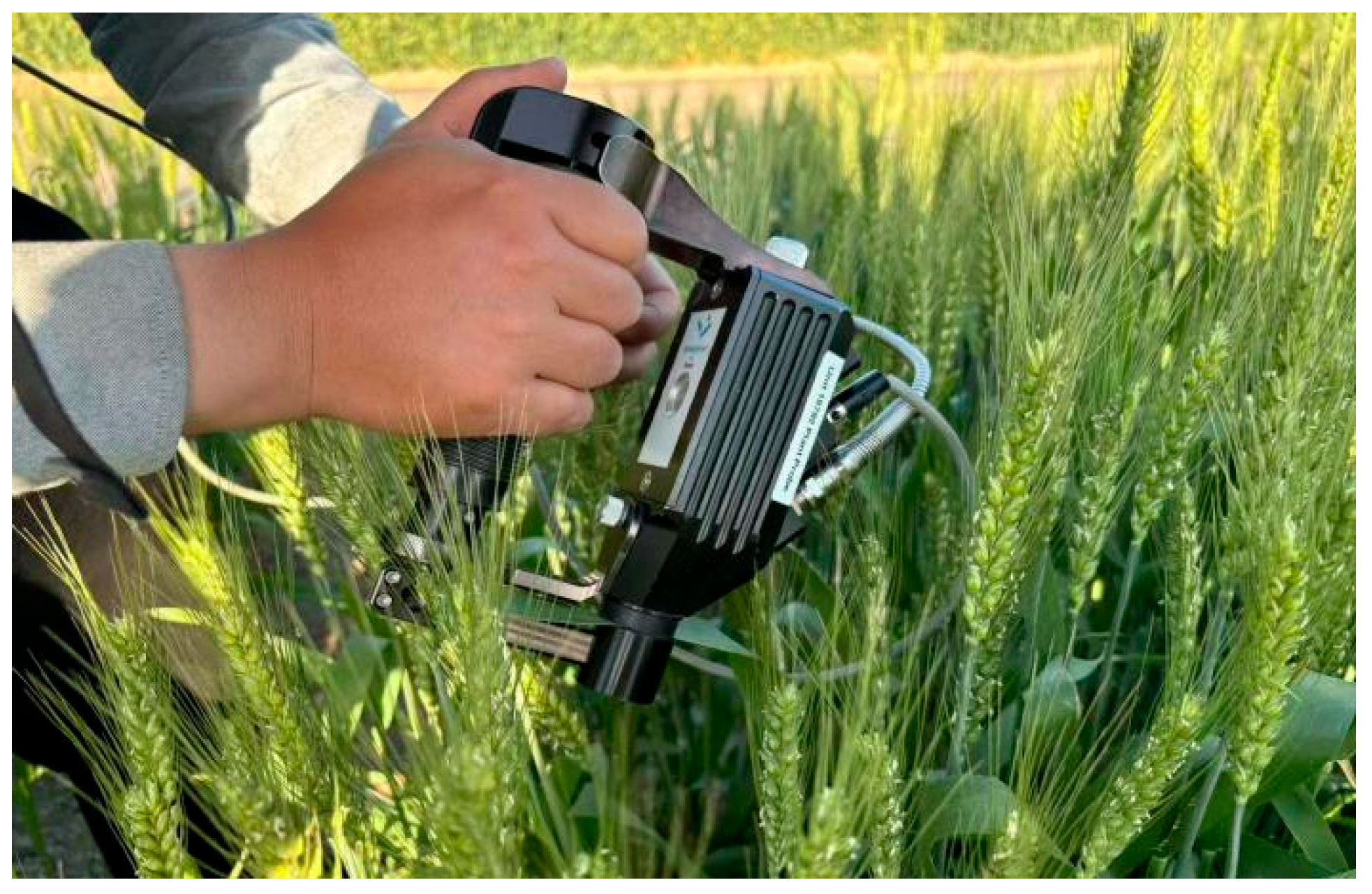
Figure 1. Photograph of non-imaging hyperspectral data acquisition at the leaf scale.
Remotesensing 17 03304 g001
Figure 2. Lesion symptoms of wheat powdery mildew, stripe rust, and leaf rust.
Remotesensing 17 03304 g002
Figure 3. Wheat leaves with different severity levels of strip rust. From left to right, the disease severity levels are 0%, 1%, 5%, 10%, 20%, 40%, 60%, 80%, and 100%.
Remotesensing 17 03304 g003
Figure 4. Distribution of disease severity data in different years for powdery mildew, leaf rust, and stripe rust. Note: “***” represents a significant difference with p < 0.0001, while “ns” represents no significant difference.
Remotesensing 17 03304 g004
Figure 5. CWA features discriminative power p-value, graphed by decomposition scale and wavelength.
Remotesensing 17 03304 g005
Figure 6. Accuracy of classification of three wheat foliar diseases using top-ranked (1%, 5% and 10%) CWA-based features, combined with three machine learning models.
Remotesensing 17 03304 g006
Figure 7. Accuracy results for the classification of three wheat foliar diseases using SPA-based feature selection and machine learning models. (a) Overall Accuracy (OA) achieved by the machine learning models; (b) map-level image classification efficacy (MICE) achieved by the machine learning models.
Remotesensing 17 03304 g007
Figure 8. Accuracy results for the classification of three wheat foliar diseases using CWPA-based feature selection combined with machine learning models. (a) Overall Accuracy (OA) achieved by the machine learning models; (b) map-level image classification efficacy (MICE) achieved by the machine learning models.
Remotesensing 17 03304 g008
Figure 9. Accuracy results of classification of three wheat foliar diseases using Relief-F based feature selection combined with machine learning models. (a) Overall Accuracy (OA) achieved by the machine learning models; (b) map-level image classification efficacy (MICE) achieved by the machine learning models.
Remotesensing 17 03304 g009
Figure 10. Chlorophyll content of healthy wheat leaves and leaves stressed by three diseases.
Remotesensing 17 03304 g010
Figure 11. Spectral response of wheat leaves to infections at different disease severity levels.
Remotesensing 17 03304 g011
Figure 12. Electron microscopy images of cellular tissues in wheat leaves infected with major foliar diseases (powdery mildew, stripe rust, and leaf rust) at different severity levels.
Remotesensing 17 03304 g012
Table 1. Acquisition of leaf spectral data.
Disease TypeExperimentTimeCultivarDisease Severity (DS)Number of SamplesData Function
Powdery mildew12017–2018Nannong-0686
Nannong-9918
1–40%49Validation
40–60%29
60–100%63
42023–2024Nannong-06861–40%60Training
40–60%56
60–100%72
Stripe rust22022–2023Nannong-0686
Yangfumai-8161
Nannong-92R137
1–40%62Validation
40–60%9
60–100%4
32023–2024Nannong-0686
Yangfumai-8161
Nannong-92R137
1–40%47Training
40–60%29
60–100%28
Leaf rust22022–2023Nannong-0686
Yangfumai-8161
Nannong-92R137
1–40%25Validation
40–60%4
60–100%3
32023–2024Nannong-0686
Yangfumai-8161
Nannong-92R137
1–40%52Training
40–60%48
60–100%16
None (healthy leaves only)12017–2018Nannong-0686
Nannong-9918
0105Validation
22022–2023Nannong-0686
Yangfumai-8161
Nannong-92R137
067Validation
32023–2024Nannong-0686
Yangfumai-8161
Nannong-92R137
0248Training
Table 2. CWA feature selection classification results for wheat foliar diseases classification.
CWA Rank ThresholdNumber of FeaturesWavelength (nm) (Scale) RFKNNBAYES
OAMICEOAMICEOAMICE
1%29See Note 10.690.530.710.540.700.52
5%33See Note 20.640.460.680.500.680.52
10%50See Note 30.610.420.680.510.250.14
Note1: The top 1% sensitive wavelet feature bands (nm) and corresponding scales (unitless) are as follows: 352 (8), 357 (8), 362 (8), 367 (8), 372 (8), 377 (8), 389 (7), 402 (8), 407 (8), 412 (8), 414 (8), 419 (8), 424 (8), 435 (6), 491 (8), 496 (8), 501 (8), 506 (8), 511 (8), 516 (8), 521 (8), 526 (8), 531 (8), 536 (8), 540 (8), 543 (8), 548 (8), 553 (8), 558 (8), 1566 (6), 1634 (6), 1708 (6), 2045 (6). Note2: The top 5% sensitive wavelet feature bands (nm) and corresponding scales (unitless) are as follows: 435 (6), 521 (8), 526 (8), 531 (8), 536 (8), 540 (8), 543 (8), 548 (8), 553 (8), 554 (2), 558 (8), 563 (8), 568 (8), 573 (8), 578 (8), 583 (8), 652 (2), 884 (7), 919 (6), 995 (6), 999 (8), 1004 (8), 1009 (8), 1056 (6), 1473 (5), 1519 (6), 1566 (6), 1634 (6), 1708 (5), 2045 (6). Note3: The top 10% sensitive wavelet feature bands (nm) and corresponding scales (unitless) are as follows: 435 (6), 526 (8), 531 (8), 536 (8), 540 (8), 543 (8), 548 (8), 553 (8), 554 (2), 558 (8), 563 (8), 567 (2), 568 (8), 573 (8), 578 (8), 583 (8), 588 (8), 652 (2), 655 (1), 657 (2), 919 (6), 980 (4), 1009 (3), 1014 (8), 1019 (4), 1032 (4), 1056 (6), 1062 (4), 1075 (4), 1088 (4), 1100 (3), 1115 (4), 1132 (5), 1152 (5), 1172 (4), 1197 (6), 1246 (1), 1260 (6), 1269 (4), 1288 (4), 1309 (4), 1332 (4), 1473 (5), 1519 (6), 1566 (6), 1634 (6), 1708 (6), 1765 (5), 2045 (6), 2126 (6).
Table 3. Classification results of three wheat foliar diseases using SPA-based feature selection and machine learning models.
AlgorithmNumber of FeaturesWavelength (nm)OAMICE
RF38See Note 10.590.40
KNN32See Note 20.690.51
BAYES35See Note 30.670.50
Note1: The combination of SPA and RF models selected the wavelengths (nm) as follows: 350, 703, 1360, 1363, 1366, 1370, 1374, 1382, 1395, 1832, 1833, 1836, 1837, 1841, 1843, 1849, 1850, 1851, 1853, 1854, 1858, 1859, 1863, 1870, 1871, 1875, 1877, 1900, 1902, 1909, 1912, 1913, 1921, 2471, 2488, 2489, 2496, 2499. Note2: The combination of SPA and KNN models selected the wavelengths (nm) as follows:350, 368, 1261, 1361, 1363, 1365, 1370, 1372, 1382, 1832, 1835, 1837, 1841, 1843, 1849, 1851, 1854, 1859, 1868, 1870, 1871, 1877, 1880, 1898, 1900, 1902, 1912, 1914, 2488, 2496, 2499. Note3: The combination of SPA and BAYES models selected the wavelengths (nm) as follows:350, 540, 1084, 1361, 1362, 1363, 1366, 1370, 1382, 1832, 1835, 1837, 1841, 1843, 1849, 1850, 1851, 1853, 1854, 1859, 1861, 1870, 1876, 1880, 1895, 1900, 1902, 1907, 1912, 1914, 2488, 2489, 2496, 2500.
Table 4. Results of classification of three wheat foliar diseases using CWPA-based feature selection combined with machine learning models.
AlgorithmNumber of FeaturesWavelength (nm), (Scale)OAMICE
RF2668 (5), 894 (7)0.740.59
KNN2668 (5), 894 (7)0.770.63
BAYES2668 (5), 894 (7)0.760.62
Table 5. Results of classification of three wheat foliar diseases using Relief-F-based feature selection combined with machine learning models.
AlgorithmNumber of FeaturesWavelength
(nm)
OAMICE
RF42See Note 10.490.23
KNN39See Note 20.500.21
BAYES25See Note 30.430.16
Note1: The combination of Relief-F and RF models selected the wavelengths (nm) as follows: 354, 350, 351, 353, 355, 356, 357, 359, 358, 352, 366, 369, 367, 365, 360, 364, 368, 363, 370, 374, 372, 373, 371, 378, 379, 361, 377, 380, 382, 383, 375, 381, 389, 388, 362, 387, 384, 386, 392, 396, 385, 393; Note2: The combination of Relief-F and KNN models selected the wavelengths (nm) as follows: 354, 350, 351, 353, 355, 356, 357, 359, 358, 352, 366, 369, 367, 365, 360, 364, 368, 363, 370, 374, 372, 373, 371, 378, 379, 361, 377, 380, 382, 383, 375, 381, 389, 388, 362, 387, 384, 386, 392; Note3: The combination of Relief-F and BAYES models selected the wavelengths (nm) as follows: 354, 350, 351, 353, 355, 356, 357, 359, 358, 352, 366, 369, 367, 365, 360, 364, 368, 363, 370, 374, 372, 373, 371, 378, 379.
Table 6. Comparison of the performance of a machine learning model employing data from four feature selection algorithms.
RFKNNBAYES
AlgorithmOAMICENumber of FeaturesOAMICENumber of FeaturesOAMICENumber of Features
CWA0.690.53290.710.54290.700.5229
SPA0.590.40380.690.51320.670.5035
CWPA0.740.5920.770.6320.760.622
Relief-F0.490.23420.500.21390.430.1625
Disclaimer/Publisher’s Note: The statements, opinions and data contained in all publications are solely those of the individual author(s) and contributor(s) and not of MDPI and/or the editor(s). MDPI and/or the editor(s) disclaim responsibility for any injury to people or property resulting from any ideas, methods, instructions or products referred to in the content.