Technical Note

Variation in SCM Supply Effects as Reflected by Coupling Relationship with Pycnocline

1
State Key Laboratory of Physical Oceanography, Ocean University of China, Qingdao 266100, China
2
Laoshan Laboratory, Qingdao 266237, China
*
Author to whom correspondence should be addressed.
Remote Sens. 2025, 17(19), 3283; https://doi.org/10.3390/rs17193283
Submission received: 12 July 2025 / Revised: 20 September 2025 / Accepted: 23 September 2025 / Published: 24 September 2025

Abstract

Highlights

What are the main findings?
  • By establishing a linear regression equation between the pycnocline and the subsurface chlorophyll maximum (SCM), the monthly coupling coefficient was calculated, revealing a cyclical pattern of strengthening and weakening in their coupling relationship.
  • During periods of strong coupling, the chlorophyll profile peak consistently coincides with the particulate backscattering (BBP) profile peak, a phenomenon that has been validated through BGC-Argo observations.
What is the implication of the main finding?
  • The formation mechanisms of the SCM are not static in the corresponding regions but exhibit cyclical patterns on seasonal scales.
  • The pycnocline influences biomass accumulation by either enhancing (through efficient nutrient mixing within the pycnocline) or suppressing (by restricting nutrient exchange across the pycnocline) nutrient availability via its mixing and stratification effects. This mechanism drives the cyclical patterns observed in the formation of the SCM.

Abstract

The subsurface chlorophyll maximum (SCM) is widely observed in the ocean and is often associated with phytoplankton biomass, where aggregated phytoplankton leads to increased chlorophyll concentrations in the water column. Pycnocline facilitates biomass accumulation by trapping nutrients and providing favorable physical conditions. However, comprehensive studies remain lacking regarding the coupling mechanism between pycnocline and SCM and the extent to which this relationship affects SCM dynamics through biomass accumulation. To investigate the seasonal coupling between the pycnocline and SCM, we established a linear regression model and quantified their relationship using a coupling coefficient, which describes the seasonal transition of SCM in terms of biomass accumulation. The results were validated using BGC-Argo data. Our findings reveal that SCM and the pycnocline consistently exhibit periodic coupling patterns within seasonal cycles, and in the Indian Ocean and the northwestern Pacific, SCM is predominantly biomass-driven during seasons with strong pycnocline coupling (the coupling coefficient ranges between 0.5 and 0.7). In contrast, this coupling weakens significantly in oligotrophic regions (the coupling coefficient remained below 0.3 in more than half of the months studied), where SCM no longer exhibits a clear overlap with peaks in particulate backscattering (BBP).

1. Introduction

Subsurface chlorophyll maximum layers (SCM) is a biological thin-layer phenomenon formed by the concentration of chlorophyll distributed within phytoplankton in the ocean profile [1]. Its timescales are on the order of a day or longer, and horizontal length scales in turn range from sub-mesoscale, about 2 km, to the extent of oligotrophic biomes, more than 1000 km [2]. The formation and maintenance factors of SCM are primarily attributed to two causes: one is the chlorophyll maximum induced by the peak biomass resulting from the aggregation of phytoplankton, and the other is the photoacclimation of phytoplankton [3,4,5]. Therefore, the variation characteristics of SCM essentially reflect the response of phytoplankton to changes in the external environment [6,7]. Understanding the mechanisms behind SCM variations is of great significance for comprehending the processes of marine ecological environment changes, as well as the coupling of physical, chemical, and biological factors.
The pycnocline is often defined as a layer located beneath the mixed layer where the density varies sharply with depth [8]. Pycnocline limits the exchange of nutrients and energy between the mixed layer and the deep layer below the density transition and is closely related to primary productivity [9,10]. During this stage, the wind-heat exchange between the sea and the atmosphere is sufficient, while the water layer beneath it has not been in contact with the sea surface for a long time. Therefore, the pycnocline also marks the depth limit of the upper ocean layer [11].
There have been many conclusions regarding the formation and maintenance mechanisms of SCM, but there are no research results on its dependence on environmental changes in response to seasonal variations. Due to the different seasons, the factors that contribute to its formation and maintenance may also gradually change. The pycnocline itself can facilitate the accumulation of phytoplankton within its layer by reducing their sinking rate [12]. Additionally, the pycnocline restricts the vertical transport of nutrients, including key elements such as phosphorus and nitrogen that are essential for phytoplankton growth [13]. Some studies have even demonstrated its close association with spring blooms [14]. Furthermore, the pycnocline can create favorable biochemical conditions for phytoplankton growth and development by influencing factors such as light availability and temperature [15]. In summary, the pycnocline plays a crucial role in the biomass accumulation of phytoplankton [16]. Although existing studies have described the relationship between biomass and SCM based on the pycnocline [17], there is still a lack of research elucidating the seasonal coupling mechanisms underlying SCM formation dynamics.
To fill this gap, this paper will use the physical reanalysis dataset and the global biochemical reanalysis dataset provided by the Copernicus data website to construct a global distribution dataset of the pycnocline and SCM. The seasonal characteristics and variation features of the pycnocline and SCM in four sea regions around the world in different seasons were studied. The coupling relationship between pycnocline and SCM was described by using the linear regression model. By varying the coupling coefficients, the contribution of the pycnocline to the SCM in different seasons was described, as well as the changing trend of the causes of the SCM itself throughout the seasons. Finally, the BGC-Argo profile was matched for verification.

2. Materials and Methods

Considering the significant correlations between SCM and both the mixed layer (MLD) and bottom depth of the euphotic zone (ZEU), corresponding datasets were also established for reference.

2.1. SCM Datasets

The chlorophyll dataset was obtained from https://data.marine.copernicus.eu/product/, accessed on 9 June 2025. This dataset was generated through the application of integrated biogeochemical and ocean dynamic models (such as the PISCES and NEMO models), incorporating other information technologies, and has been extensively validated with in situ measurements. It is also widely used in marine and climate research activities and forecasting services [18,19,20]. The selected dataset has a 0.25° × 0.25° spatial resolution, a daily temporal resolution, and 50 vertical levels ranging from 0 to 5700 m, covering the global ocean.

2.2. Pycnocline Datasets

So far, most of the research on pycnocline still does not rely on directly measuring the density values in the ocean but calculates the density by measuring the temperature, salinity and depth in seawater. Therefore, we also chose the Global Ocean Ensemble Physics Reanalysis product provided by the Copernicus data website, which contains the data parameters we need [21]. Additionally, the pycnocline dataset we selected features a temporal resolution of daily and a spatial resolution of 0.25° × 0.25°, and we extracted data distributed vertically within the 0–250 m depth range as our final dataset.

2.3. ZEU Datasets

The ZEU dataset is a fusion product from four water color satellite sensors. Single-sensor and merged products from SeaWiFS, MERIS, MODIS, VIIRS NPP, OLCI-A, VIIRS JPSS-1, and OLCI-B. The data was calculated using the chlorophyll concentration empirical algorithm. The Daily ZEU dataset is a data product provided by GlobColour.

2.4. Data Processing

2.4.1. SCM Processing

Chlorophyll profiles with SCM characteristics in the ocean generally present a single-peak structure, and in the SCM datasets, chlorophyll has a unified depth structure in the profile (with high accuracy in the first 250 m and then decreasing successively). Therefore, when extracting SCM data, the Gaussian fitting function is used to extract the complete chlorophyll profile parameters, including depth, thickness and intensity (Figure 1). If Z represents depth, then the chlorophyll concentration fitted by Gaussian at Z ( C h l a ( Z ) ) should be expressed as
C h l a Z = B 0 + A e ( Z Z m a x ) 2 2 σ 2
In the Gaussian fitting function, B 0 represents the baseline parameter, A represents the peak or amplitude of the Gaussian curve, Z m a x indicates the position of the amplitude, σ represents the standard deviation of the Gaussian curve. If the parameters of the Gaussian fitting function are converted into SCM characteristics, B 0 represents the chlorophyll level of the subsurface background constant, A represents the peak of chlorophyll concentration, Z m a x represents the maximum depth of chlorophyll concentration, and 2 σ represents the thickness of SCM [22]. In the previous process of identifying SCM profiles by BGC-Argo, complex profile processing and error correction processes would be experienced [23,24,25]. By using Gaussian curve fitting, SCM can be judged and extracted directly through the changes in mathematical parameters, and the process is more concise and effective.

2.4.2. Pycnocline and MLD Processing

First, the density needs to be calculated based on the parameters such as temperature, salinity and depth contained in the original dataset according to the Thermodynamic Equation of Seawater 2010 (TEOS-10) equation [26,27]. In this study, the water depth of most of the studied sea region exceeded 200 m. Therefore, the suggestions of the earlier oceanographic survey [28,29] were adopted, and the density gradient value of 0.015kg/m3 was selected as the determination criterion for the pycnocline. The determination criterion of the mixed layer uses the classic density threshold method, and the mixed layer is determined by determining the threshold difference between the deeper water level and the near-surface water level [30].

2.4.3. BGC-Argo Processing

We initially conducted preliminary screening of profiles based on the geographical location of each region. Selected float profiles were required to possess both Chl-a fluorometer and BBP sensors. Furthermore, the BBP profiles underwent sequential processing steps including dark signal correction, spike removal, and instrument drift adjustment. The sensor fluorescence data were also converted to chlorophyll-a concentrations through necessary procedures, with detailed methodologies referenced in Bellacicco et al. [31].

3. Results

Before describing the relationship between the pycnocline and SCM, we first need to understand the characteristics of SCM and the pycnocline themselves, including their range scale, duration, and the proportion of influence of each parameter, as well as seasonal characteristics and global distribution features, etc.

3.1. Global Distribution of the Pycnocline and SCM

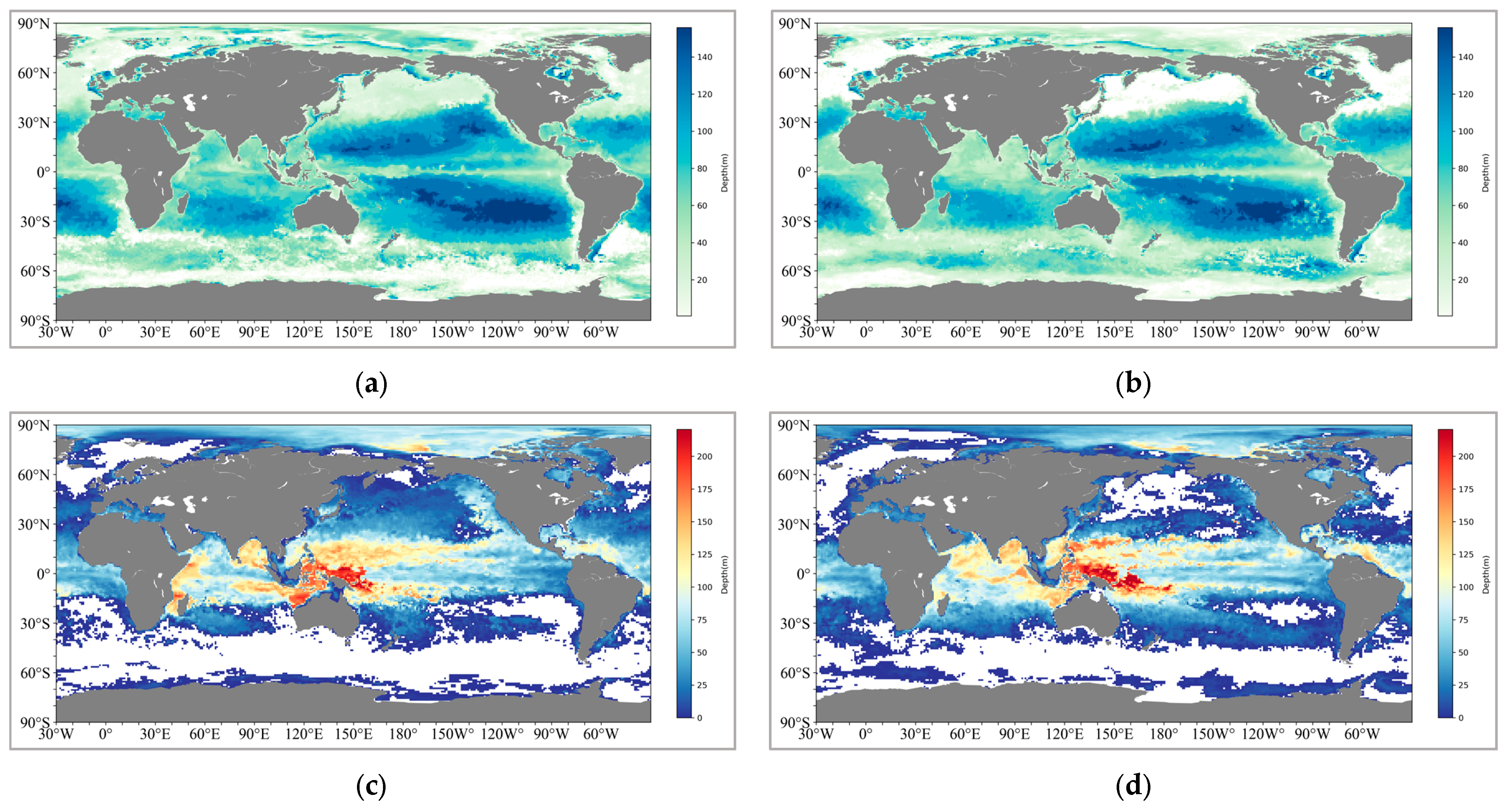
Globally, the depth of the SCM in nearshore waters is generally around 60 m. With increasing convergence with land, the depth of SCM in oceanic waters can reach 140 m. In terms of distribution structure, the depth distribution of SCM in the North and South Pacific is separated by the equator, forming two independent bowl-shaped structures. In terms of seasonal variations, SCM is not obvious in changes between winter and summer in either hemisphere (Figure 2a,b). The results of these data and structures are also in line with the current observational results and numerical simulations for global sea regions [4,32].
As for the pycnocline, it is most reasonable to use thickness as an element to describe its explanation of the morphology and changes in the mode water structure on a global scale [33]. Its characteristics on the horizontal scale are opposite to those of SCM. The thicker regions are often closer to the continental coast, and the thickest regions can reach 200 m. When viewed along the latitude zone, it shows obvious regional characteristics. The thickness is the greatest at the equator, while it gradually decreases to about 120 m near the subtropical circulation until it becomes less than 50 m as the latitude increases. In addition, the thickness of the pycnocline is significantly affected by seasonal variations. Under the same latitude conditions, the thickness of the pycnocline in the Northern Hemisphere during summer is more easily detected and thicker, and correspondingly, there is the same variation trend in the Southern Hemisphere (Figure 2c,d).

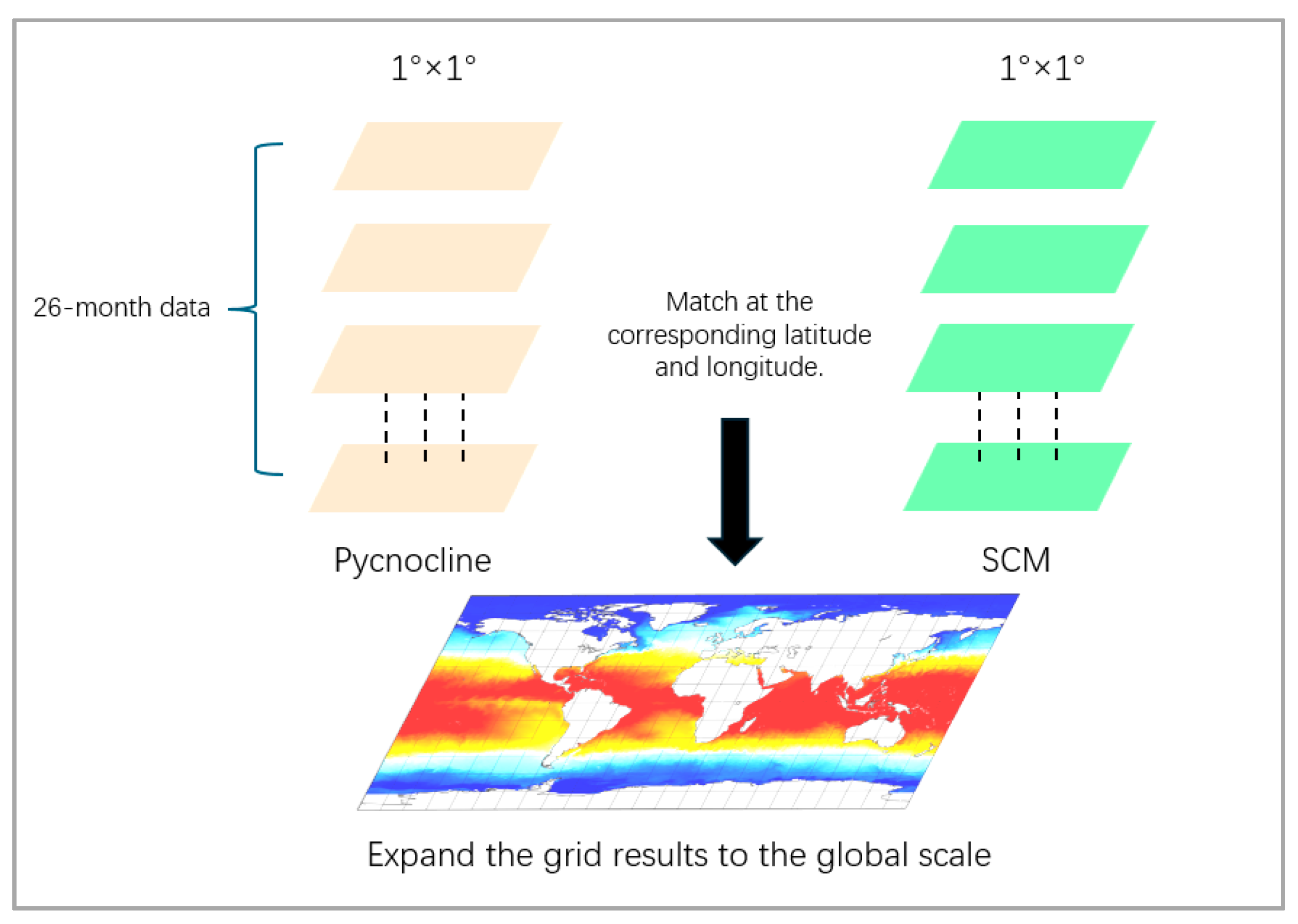
3.2. The Coupling Result of 1° Grid Matching SCM and Density Layering

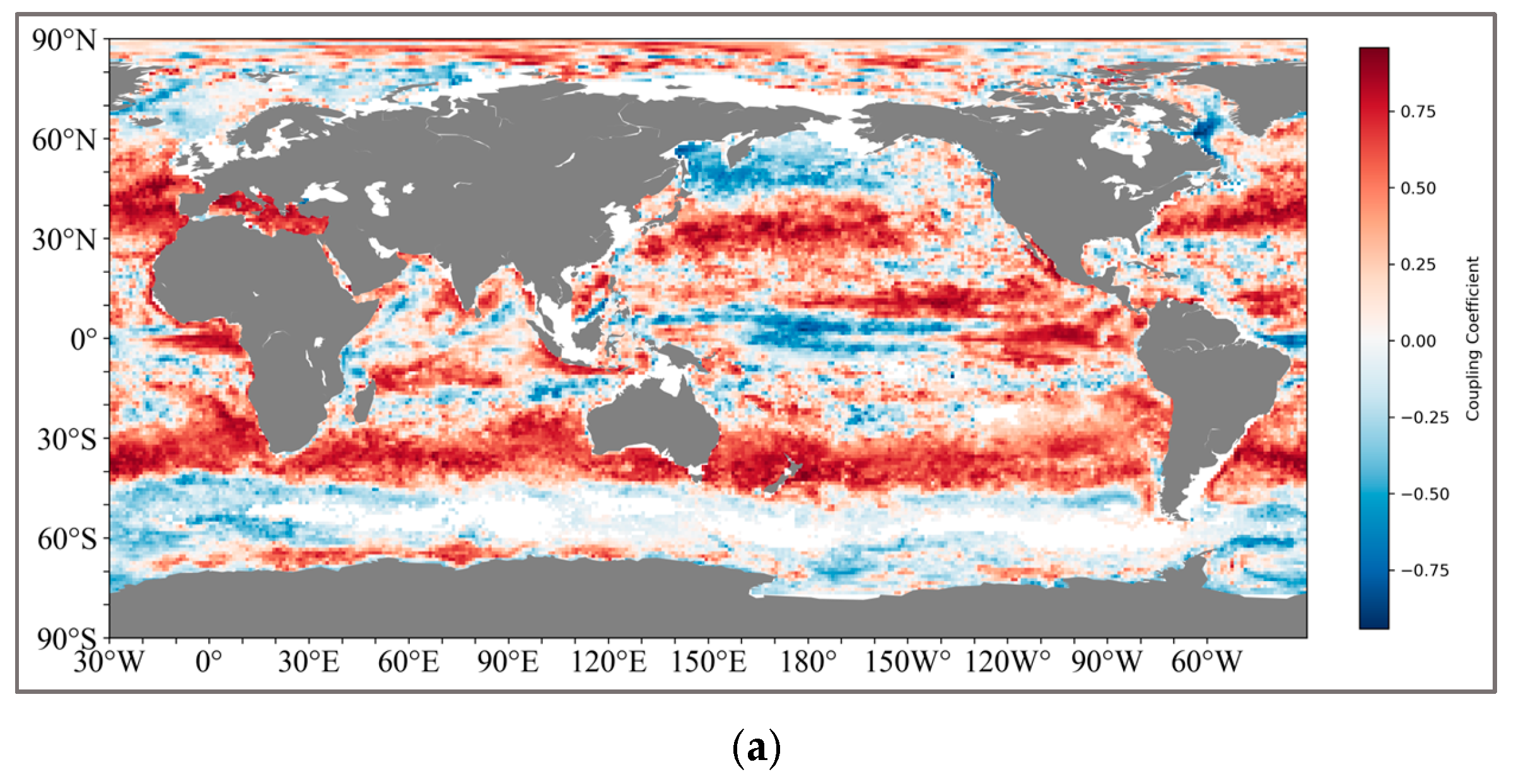
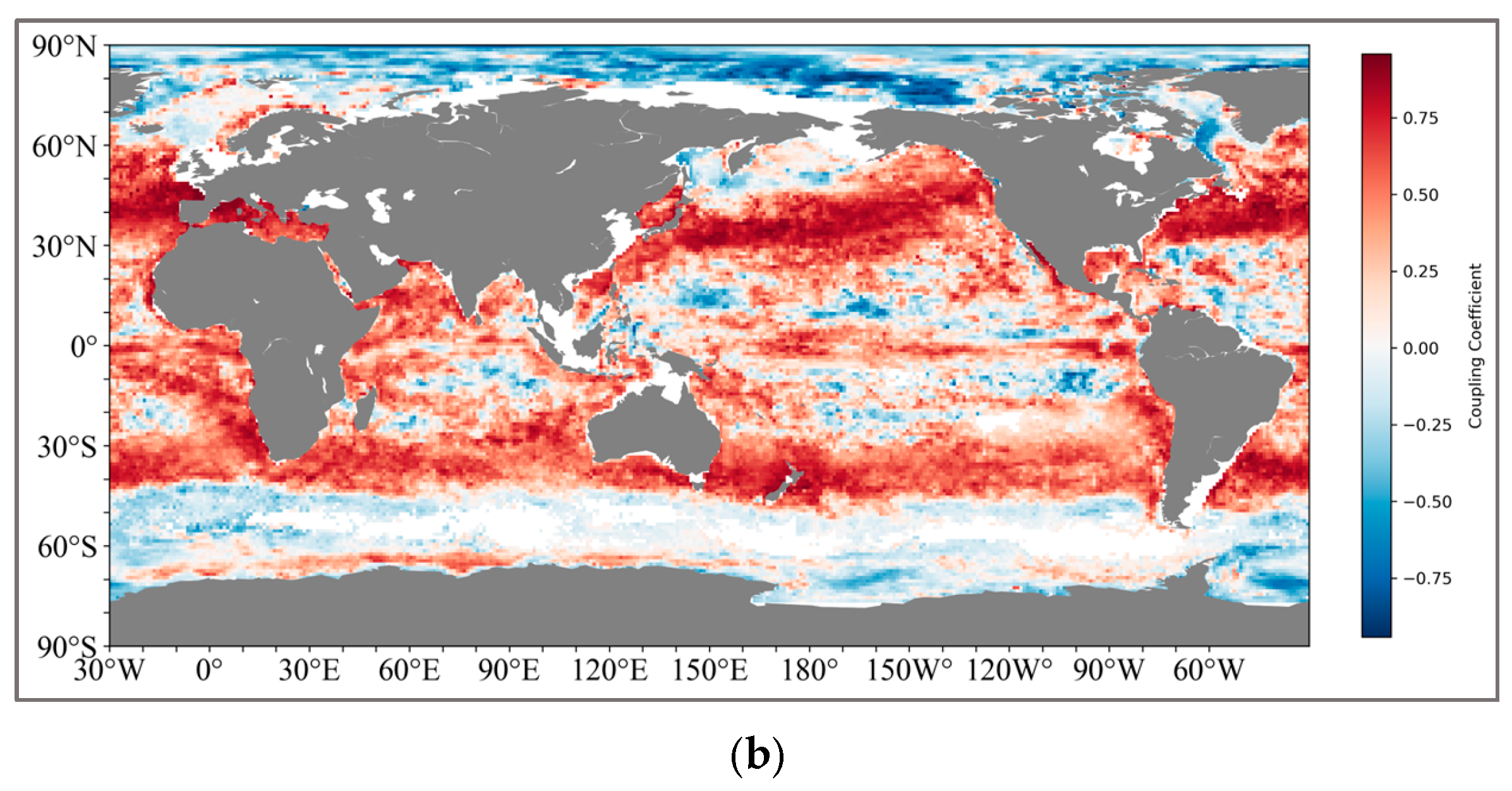
The calculation method is shown in Figure 3. We ultimately retained two sets of global coupled calculation results, one being the thickness of the pycnocline and SCM, and the other being the depth of the maximum rate of the density and SCM (Figure 4). For the results of the thickness coupling, SCM and pycnocline show a very broad positive correlation in both the northern (20°N–50°N) and southern (30°S–42°S) subtropical regions. The coupling coefficient in the northern subtropical region reaches the highest at 45°N, with the correlation performance above 0.8, and decreases on both sides all the way to the mid-high latitude region of 60°N and the near-equator region of 15°N. In the Southern Hemisphere, the coupling coefficient is relatively lower than that in the Northern Hemisphere, and there are no highly coupled regions.
The positively coupled regions formed near the South Pacific and the South Atlantic present a symmetrical structure like that of the Northern Hemisphere.
For the coupling results of the pycnocline with the maximum change rate and SCM, the coupling relationship between the two is obviously not as tight as that of the thickness. Although there is still a positive coupling correlation in the South Pacific and the South Atlantic (25°S–40°S), the coupling coefficients generally fluctuate around 0.5. However, in the middle and high latitudes of the North Pacific (45°N–65°N), a negative correlation is shown.
Finally, we divide the global sea regions into the following several regions for subsequent research: Indian Ocean (IO), Northwest Pacific (NWP), Southeast Pacific (SEP), North Atlantic (NA), South Atlantic (SA).

3.3. Seasonal Coupling Relationship

To evaluate the relative contributions of the three pycnocline parameters to the formation of the SCM, we designed a linear regression equation based on the least squares method. This approach leverages the inherent adaptability and robustness of the least squares algorithm to integrate variation trends across variables with different units and determine the most appropriate weighting coefficients. Finally, the coupling coefficient of the equation is used to represent the overall correlation between the pycnocline and the SCM.
S C M i = ω 1 · T h i c k n e s s + ω 2 · I n t e n s i t y + ω 3 · D e p t h
Among them, S C M represents the depth corresponding to the maximum chlorophyll content in each 1° × 1° grid section. Thickness represents the thickness of the pycnocline, measured in meters, and the value selected is the difference between the upper and lower boundaries of the pycnocline. Intensity refers to the peak value of the intensity in the pycnocline profile, measured in milligrams per cubic meter. Depth represents the depth at which the density change rate is the greatest, also measured in meters, and it is used to correspond with the position of the maximum value of chlorophyll. ω represents the weight coefficient. In the selected region, we use the above equation as the way to describe the parameters of SCM. To verify the accuracy of the results, we matched similar BGC-Argo data on a temporal and spatial scale, which serves as an important reference for a more detailed description of the seasonal variation process.
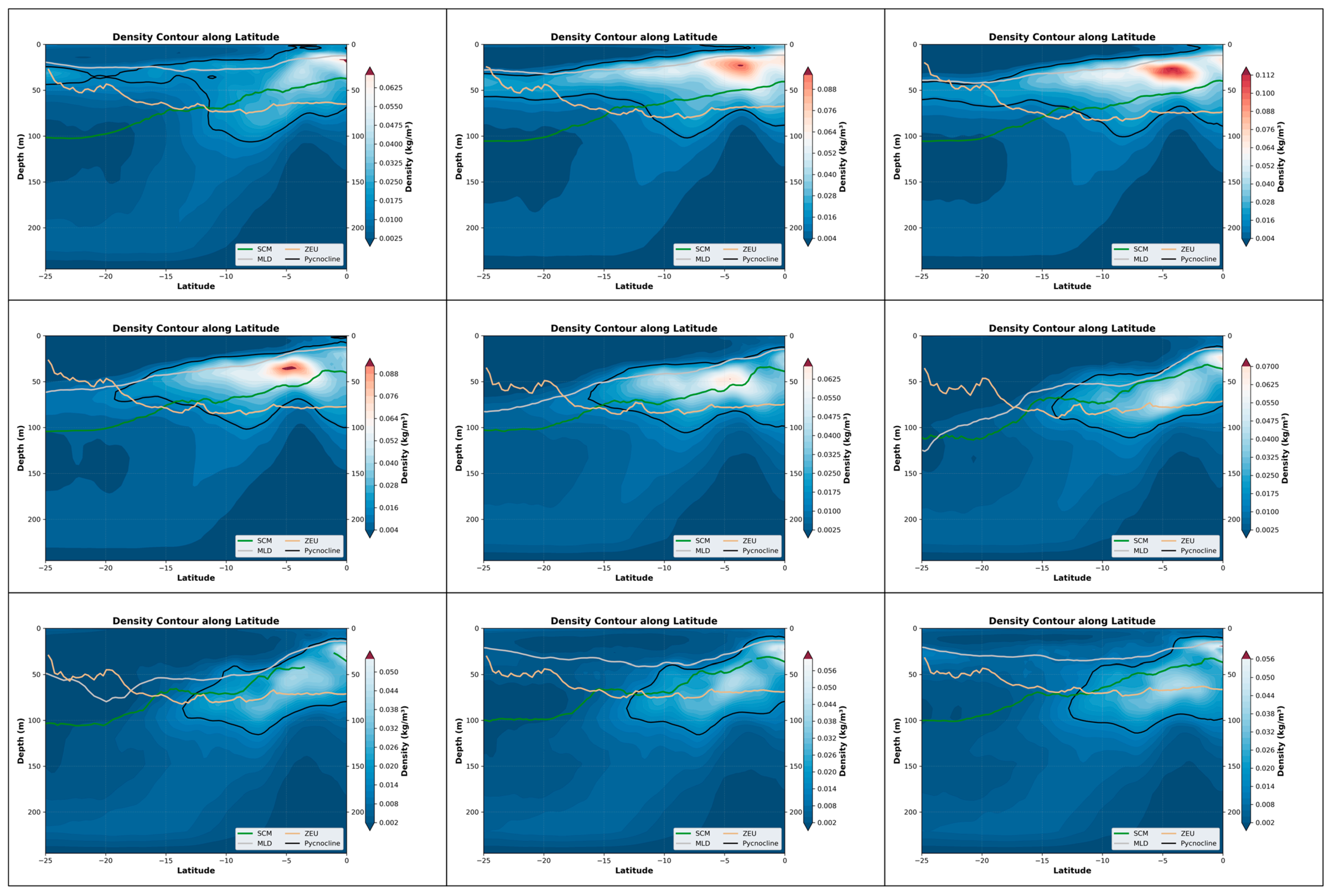
Furthermore, within the selected region, we calculated the variations in MLD, ZEU, and the pycnocline along the latitude direction for each 1° after statistics, and they varied by month.

3.3.1. Indian Ocean Region

In the Indian Ocean region, among the three parameters of the pycnocline, thickness holds an absolute dominant position in terms of its contribution to SCM. In addition, its coupling mode varies significantly with the seasons. They reached the highest level of 0.678 in April, then gradually decreased until September, and then gradually began to rise until the cycle was completed within one year (Table 1).
From the perspective of the cross-sectional structure, there has always been a stable stratified water mass near the equator, distributed at a depth of approximately 50 m to 150 m. Overall, during the June–August winter period, the SCM exhibited a slight upward shift, albeit modest (approximately 15 m). Concurrently, the coupling relationship between the SCM and the pycnocline also weakened over the same timeframe (Figure 5). This suggests that the accumulation of phytoplankton in the upper layer during this season may not be primarily driven by biomass. Only in the southern latitudes, it may fluctuate and float due to the influence of the equatorial ocean current with different temperatures in winter and summer. Combined with the SCM equation, when it is April, the thickness of the density stratum in the Indian Ocean region at this time increases significantly to 125 m, and the distribution is uniform. Meanwhile, the higher density change rate of the water mass within the equator also shows a good mixing effect, and an obvious supply trend is also shown in the equation. In the BGC-Argo profile, it can also be observed that in April, the SCM showed a significant upward trend. At this time, the peak signals of SCM and BBP were highly overlapping, indicating that at this point, biomass was the dominant factor (Figure 6).

3.3.2. Northwest Pacific Region

In the Northwest Pacific region, no strongly pronounced coupling peak was observed throughout the year, with all coupling coefficients remaining below 0.6. The overall trend indicates that the coupling intensity was highest in winter, followed by a gradual decrease through spring and summer, reaching its lowest point in autumn at approximately 0.2 (Table 2). Compared to other regions, the coupling relationship between the pycnocline and the SCM remained relatively stable with minimal fluctuations, suggesting that the water mass within the pycnocline consistently provides effective nutrient support to the SCM.
In the Northwest Pacific Ocean, the seasonal characteristics of the pycnocline are more pronounced. Among them, the seasonal clump is most intense in August and September, when the upper water mass mixes most intensely. Then, as the temperature gradually drops, the density clump near the mid-latitudes begins to dissipate, and the efficiency of water and heat exchange between seawater decreases. It is not until March and April, when the temperature rises, that the cycle starts again (Figure 7). From the perspective of the coupling relationship, it is better during the period when the sea surface water mass is more stable. Unlike the situation in the Indian Ocean, where SCM is always within the stable water mass, the mixing process on the sea surface in the North Pacific always occurs above SCM. This might be the reason why the coefficient-intensity relationship is negative when the seawater mixing is the most intense. This indicates that seawater mixing currently has always been an unfavorable factor affecting the formation of SCM. Furthermore, similar situations can also be observed from the BGC-Argo profiles. In August, when the density stratification layer indicates the strongest mixing of seawater, the intensity of SCM is relatively low and its thickness is thinner. It is not until December that a distinct peak signal coupled with SCM is observed in BBP, which is like the change in the coupling coefficient of the equation (Figure 8).

3.3.3. Southeast Pacific Region

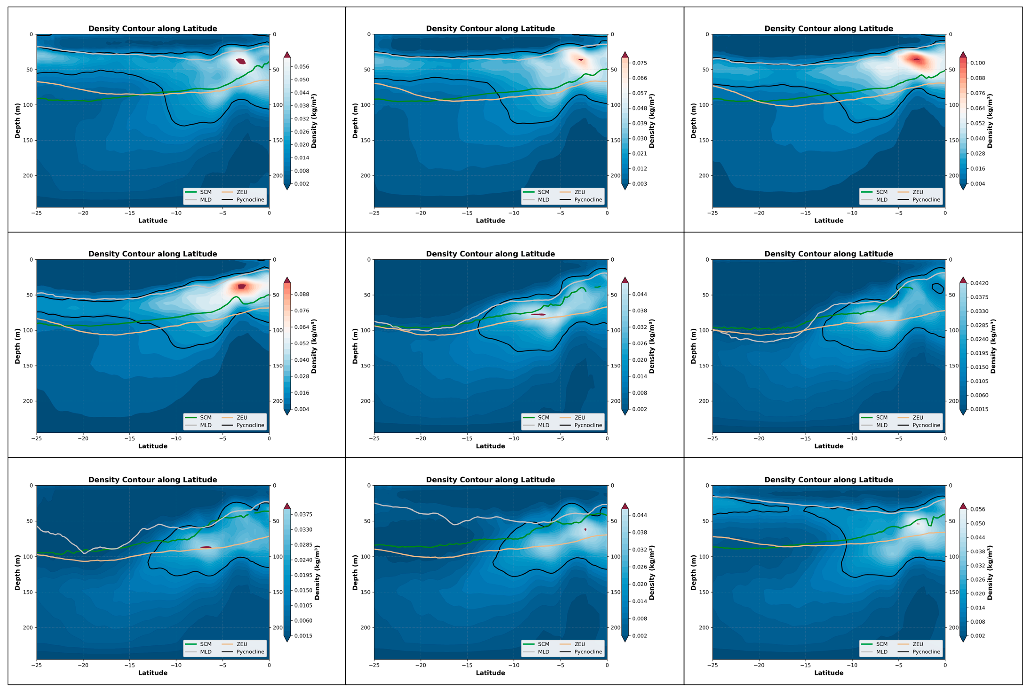
The coupling relationship within the Southeast Pacific Ocean is different from the supply effect in the previous sea region. On the contrary, from the perspective of the coupling coefficient, the highly mixed water mass formed within the pycnocline is more like a limiting factor of SCM. The seasonal variation among the coupling coefficients is not obvious. Only from February to April does it show a significant negative correlation trend (Table 3). Currently, the seasonal density transition layer is widely present in the mid- and low-latitude regions, with the strongest mixture in seawater and the most intense impact on SCM. Like in the Northwest Pacific, the depth range of the SCM is still below the maximum value of density change. Similarly, a similar negative value has also appeared in the strength of the coupling coefficient, showing similar results as before. The seasonal variation in SCM is relatively stable. Overall, it shows a trend of being deep in the mid-latitudes and shallow in the low latitudes. Considering the morphology of water masses, this change seems more like the result of being lifted under the dynamic environment. This means that, in the low-latitude range near the equator, although the distribution of SCM is shallower, it is also more unstable (Figure 9). The influence of seawater disturbances is not conducive to the formation and maintenance of SCM. In the BGC-Argo profile, the intensity value of SCM is significantly lower than that in previous sea regions. Moreover, during the seasonal changes, its variation is not as obvious as that in the previous profiles, and the seasonal characteristics are relatively weak. From the perspective of BBP, there is a phenomenon where the peaks of the two coincide only in February, March, June, and July. Although the coupling result is like the equation, upon closer examination, it can be observed that the two peaks are not completely overlapping. The depth of SCM is deeper, and overall, the peak signal of BBP itself is not obvious (Figure 10). This perhaps explains the low overall coupling between the two and the relatively weak overall intensity of SCM.

3.3.4. South Atlantic Region

The seasonal coupling relationship in the South Atlantic is the strongest, reaching above 0.7 in April and May. There is a brief transition period in June, during which the coupling relationship begins to decline. By July and beyond, the formation of SCM and the water masses in the upper sea surface no longer have a strong correlation until the seasonal pycnocline layer re-forms. Furthermore, as shown by the equation, the reason for the high coupling in April-May is that the depth of the maximum density change rate is closely related to the height of the SCM (Table 4). Moreover, in the latitude profile chart for April-May, it can be clearly observed that the SCM near 5° south latitude and the lower boundary of the density layer have indeed shown a significant upward movement (Figure 11).
In the BGC-Argo profile, the overall strength of the SCM is relatively low, but it is relatively stable, and its thickness can reach approximately 75 m. Similarly, the BBP also did not show any significant peak signal changes throughout the season. During the period from March to May, both would experience a brief decline together, but overall, the coupling was not very tight (Figure 12).

4. Discussion

This study aims to describe the changing characteristics of the causes of SCM within different regions over the course of a season and to analyze the changes in its dependence on nutrients based on these changing characteristics. Results show that the SCM exhibits seasonal coupling with the pycnocline across different oceanic regions, consistently following a pattern of intensified coupling followed by gradual weakening over time. The seasonal pycnocline reflects dynamic mixing below the mixed layer, which is closely linked to nutrient transport and heat exchange [10]—key factors influencing biomass accumulation. The formation and maintenance of SCM are governed by the interplay between phytoplankton biomass and photoacclimation [3,5,6,34]. The observed periodic variations in coupling strength with the seasonal pycnocline indicate that the dominant control over the SCM—whether by phytoplankton biomass or photoacclimation—also shifts cyclically throughout the year.
In the Indian Ocean, the coupling between the SCM and the pycnocline reaches its peak intensity during March-April, when the region remains under the influence of the northeast monsoon. During this period, nutrient-rich waters are transported from coastal regions to the open ocean, providing essential conditions for phytoplankton biomass accumulation. Within the relatively stable water mass of the pycnocline, the moderate density gradient enables phytoplankton to access nutrients not only through vertical mixing from deeper layers but also via lateral isopycnal mixing [35]. This dual nutrient acquisition mechanism contributes to the strong SCM-pycnocline coupling observed in spring. By summer (June–September), the southwest monsoon induces a basin-scale redistribution of surface waters, with equatorial waters moving toward the Arabian Sea. This circulation shift reduces nutrient availability, leading to diminished biomass aggregation. As upwelling nutrients become scarce, SCM gradually shoals to optimize light availability through photoacclimation [6]. This vertical migration partially decouples the SCM from the pycnocline, while enhanced stratification further restricts vertical nutrient flux [36]. These combined effects ultimately weaken the SCM-pycnocline coupling.
In the Northwest Pacific, the SCM is no longer primarily sustained by nutrient supply from stable pycnocline-enclosed water masses but rather influenced more significantly by the seasonally variable pycnocline. During winter months when the pycnocline remains relatively stable, phytoplankton experience substantial proliferation. The downward movement of ocean currents facilitates nutrient uptake from deeper layers, triggering biomass accumulation and occasionally leading to spring blooms [36]. The summer regime exhibits markedly different dynamics: intensified mixing within the seasonal pycnocline disrupts phytoplankton aggregation and biological activity, creating unfavorable conditions for SCM development. During this period, the SCM formation mechanism shifts from biomass dominance to alternative controlling factors, particularly photoacclimation processes.
The Southeast Pacific Ocean represents a classic oligotrophic marine ecosystem [37], characterized by limited biomass accumulation. In this nutrient-depleted environment, the formation of SCM becomes predominantly governed by photoacclimation processes [3]. This fundamental difference explains why the pycnocline-SCM coupling in this region is significantly weaker compared to the previously discussed basins. Notably, the Southeast Pacific SCM exhibits relatively small seasonal intensity variations, manifesting primarily as vertical depth oscillations. Furthermore, the peak BBP signals are consistently confined to the upper 75 m layer, with their vertical distributions showing no temporal coincidence with SCM depth maxima across seasons. These collective observations demonstrate the light-driven nature of SCM development in oligotrophic waters, where photoacclimation overwhelmingly dominates over biomass-mediated controls.
The South Atlantic Ocean exhibits the most pronounced seasonal variability among the studied regions, with clear observational evidence of pycnocline-mediated modulation of the subsurface chlorophyll maximum (SCM). Both the equatorial Pacific and Atlantic are recognized as typical upwelling systems, demonstrating remarkably similar surface chlorophyll distribution patterns. Vertical profiles further reveal analogous seasonal distributions between these regions, with neither showing significant chlorophyll intensity variations. Notably, the BBP peaks generally remain decoupled from the SCM throughout the seasonal cycle; this indicates that it is likely to be dominated by photoacclimation for the majority of the time.

5. Conclusions

The formation and maintenance mechanisms of the SCM have been extensively discussed and studied. Among these, SCM driven by phytoplankton aggregation represents a highly important category. However, our study reveals that the supply effect of phytoplankton aggregation on the SCM may vary periodically over seasonal scales, in which the pycnocline plays a significant role. Our specific conclusions are as follows:
(1)
The relative importance of the factors governing the formation and maintenance of the SCM on a seasonal scale is not static but is seasonally dependent.
(2)
Phytoplankton aggregation consistently plays a significant role in the seasonal cyclical variations in the SCM across various marine regions.
(3)
The pycnocline influences the distribution of nutrients and the activity of phytoplankton in the ocean through cyclical seasonal variations, thereby affecting the formation and maintenance of the SCM and leading to periodic fluctuations in the strength of their coupling.
The formation mechanisms of the SCM are undoubtedly highly complex, with mesoscale dynamic processes, human activities, and the migratory behavior of phytoplankton itself all serving as significant influencing factors. In this study, the coupling relationship between pycnocline and SCM as a reference for its formation mechanism has certain limitations, and the validation approach using BGC-Argo data also presents shortcomings. In the future, we will focus on more detailed quantification of this process, assessing the impact of environmental changes on phytoplankton, and employing artificial intelligence or large-scale models to more accurately predict these variations. The findings of this study will also contribute to a better understanding of the connections and transformations among different ocean layers, thereby enhancing our knowledge of marine biogeochemical processes.

Author Contributions

Conceptualization, methodology, J.Y. and Y.H.; data curation, formal analysis, investigation, software, validation, writing—original draft, Y.H.; writing—review and editing J.Y., M.H., L.F. and Y.H.; funding acquisition, project administration, resources, Supervision, J.Y. All authors have read and agreed to the published version of the manuscript.

Funding

This research was funded by the National Natural Science Foundation of China (Grant No. 42530404) and the Laoshan Laboratory Science and Technology Innovation Projects (No. LSKJ202201302).

Data Availability Statement

BGC-Argo data used in this study are available at https://biogeochemical-argo.org/data-access.php, accessed on 4 January 2025. Global biochemical reanalysis data are available at https://data.marine.copernicus.eu/product/GLOBAL_ANALYSISFORECAST_BGC_001_028/description, accessed on 9 June 2025. Temperature, salinity and depth data are available at https://data.marine.copernicus.eu/product/GLOBAL_MULTIYEAR_PHY_ENS_001_031/description, accessed on 13 January 2025. ZEU data are available at https://hermes.acri.fr/index.php, accessed on 21 April 2025.

Conflicts of Interest

The authors declare no conflicts of interest.

References

  1. Cowles, T.J. Planktonic layers: Physical and biological interactions on the small scale. In Handbook of ScalingMethods in Aquatic Ecology: Measurement, Analysis, Simulation; Seuront, L., Strutton, P.G., Eds.; CRC Press: Boca Raton, FL, USA, 2003; pp. 31–49. [Google Scholar]
  2. Lévy, M. The Modulation of Biological Production by Oceanic Mesoscale Turbulence. In Transport and Mixing in Geophysical Flows; Weiss, J.B., Provenzale, A., Eds.; Lecture Notes in Physics; Springer: Berlin/Heidelberg, Germany, 2008; p. 744. [Google Scholar]
  3. Cornec, M.; Claustre, H.; Mignot, A.; Guidi, L.; Lacour, L.; Poteau, A.; D’Ortenzio, F.; Gentili, B.; Schmechtig, C. Deep chlorophyll maxima in the global ocean: Occurrences, drivers and characteristics. Glob. Biogeochem. Cycles 2021, 35, e2020GB0067590. [Google Scholar] [CrossRef] [PubMed]
  4. Masuda, Y.; Yamanaka, Y.; Smith, S.L.; Hirata, T.; Nakano, H.; Oka, A.; Sumata, H. Photoacclimation by phytoplankton determines the distribution of global subsurface chlorophyll maxima in the Ocean. Commun. Earth Environ. 2021, 2, 128. [Google Scholar] [CrossRef]
  5. Cornec, M.; Laxenaire, R.; Speich, S.; Claustre, H. Impact of mesoscale eddies on deep chlorophyll maxima. Geophys. Res. Lett. 2021, 48, e2021GL093470. [Google Scholar] [CrossRef]
  6. Cullen, J.J. Subsurface Chlorophyll Maximum Layers: Enduring Enigma or Mystery Solved? Annu. Rev. Mar. Sci. 2015, 7, 207–239. [Google Scholar] [CrossRef]
  7. Halsey, K.H.; Jones, B.M. Phytoplankton strategies for photosynthetic energy allocation. Annu. Rev. Mar. Sci. 2015, 7, 265–297. [Google Scholar] [CrossRef]
  8. Chu, P.C.; Fan, C. Exponential leap-forward gradient scheme for determining the isothermal layer depth from profile data. J. Ocean 2017, 73, 503–526. [Google Scholar] [CrossRef]
  9. Sharples, J. Investigating the seasonal vertical structure of phytoplankton in shelf seas. Mar. Models 1999, 1, 3–38. [Google Scholar] [CrossRef]
  10. Kawai, Y.; Hosoda, S.; Uehara, K.; Suga, T. Heat and salinity transport between the permanent pycnocline and the mixed layer due to the obduction process evaluated from a gridded Argo dataset. J. Ocean 2021, 77, 75–92. [Google Scholar] [CrossRef]
  11. Sprintall, J.; Cronin, M. Upper Ocean Vertical Structure. Encycl. Ocean Sci. 2010, 6, 3120–3128. [Google Scholar]
  12. Parslow, J.S.; Boyd, P.W.; Rintoul, S.R.; Griffiths, F.B. A persistent subsurface chlorophyll maximum in the Interpolar Frontal Zone south of Australia: Seasonal progression and implications for phytoplankton-light-nutrient interactions. J. Geophys. Res. Ocean 2001, 106, 31543–31557. [Google Scholar] [CrossRef]
  13. Fleur, C.D.; Vincent, P.; Boris, M.B.; Victor, B.; Petra, V.; Erik, M.; Paul, K.; Mark, J.A.V. Composition and distribution of the near-shore waters bordering the coral reefs of Aruba, Bonaire, and Curaçao in the Southern Caribbean. Mar. Pollut. Bull. 2024, 209, 117297. [Google Scholar] [CrossRef]
  14. Richardson, K.; Christoffersen, A. Seasonal distribution and production of phytoplankton in the southern Kattegat. Mar. Ecol. Prog. Ser. 1991, 78, 217–227. [Google Scholar] [CrossRef]
  15. Peng, X.; Yuguang, L.; Gang, L.; Qing, X.; Haibo, Z.; Zengrui, R.; Xiaobin, Y.; Fei, C. Deriving depths of deep chlorophyll maximum and water inherent optical properties: A regional model. Cont. Shelf Res. 2009, 29, 2270–2279. [Google Scholar] [CrossRef]
  16. Jang, P.G.; ALee, T.S.; Kang, J.H.; Shin, K. The influence of thermohaline fronts on chlorophyll a concentrations during spring and summer in the southeastern Yellow Sea. Acta Oceanol. Sin. 2013, 32, 82–90. [Google Scholar] [CrossRef]
  17. Wei, G.; Zhenyan, W.; Kainan, Z. Controlling effects of mesoscale eddies on thermohaline structure and in situ chlorophyll distribution in the western North Pacific. J. Mar. Syst. 2017, 175, 24–35. [Google Scholar] [CrossRef]
  18. Ciliberti, S.A.; Grégoire, M.; Staneva, J.; Palazov, A.; Coppini, G.; Lecci, R.; Peneva, E.; Matreata, M.; Marinova, V.; Masina, S.; et al. Monitoring and Forecasting the Ocean State and Biogeochemical Processes in the Black Sea: Recent Developments in the Copernicus Marine Service. J. Mar. Sci. Eng. 2021, 9, 1146. [Google Scholar] [CrossRef]
  19. Fennel, K.; Gehlen, M.; Brasseur, P.; Brown, C.W.; Ciavatta, S.; Cossarini, G.; Crise, A.; Edwards, C.A.; Ford, D.; Friedrichs, M.A.M.; et al. Advancing Marine Biogeochemical and Ecosystem Reanalyses and Forecasts as Tools for Monitoring and Managing Ecosystem Health. Front. Mar. Sci. 2019, 6, 89. [Google Scholar] [CrossRef]
  20. Ford, D.; Kay, S.; McEwan, R.; Totterdell, I.; Marion, G. Marine Biogeochemical Modelling and Data Assimilation for Operational Forecasting, Reanalysis, and Climate Research. In New Frontiers in Operational Oceanography; Createspace Independent Pub: Scotts Valley, CA, USA, 2018; pp. 625–652. [Google Scholar]
  21. E.U. Copernicus Marine Service Information (CMEMS); Marine Data Store (MDS). Global Ocean Ensemble Physics Reanalysis; Mercator Ocean International: Toulouse, France, 2024. [Google Scholar] [CrossRef]
  22. Yu, Y.; Huang, B.; Radenkovic, M.; Wang, T.; Chen, G. Intelligent Sparse2Dense Profile Reconstruction for Predicting Global Subsurface Chlorophyll Maxima. IEEE Trans. Geosci. Remote Sens. 2024, 62, 4211013. [Google Scholar] [CrossRef]
  23. Xing, X.; André, M.; Claustre, H.; Antoine, D.; D’Ortenzio, F.; Antoine, P.; Mignot, A. Combined processing and mutual interpretation of radiometry and fluorimetry from autonomous profiling Bio-Argo floats: Chlorophyll a retrieval. J. Geophys. Res. 2011, 116, C06020. [Google Scholar] [CrossRef]
  24. Xing, X.; Claustre, H.; Blain, S.; D’Ortenzio, F.; Antoine, D.; Ras, J.; Guinet, C. Quenching correction for in vivo chlorophyll fluorescence acquired by autonomous platforms: A case study with instrumented elephant seals in the Kerguelen region (Southern Ocean). Limnol. Oceanogr. Methods 2012, 10, 483–495. [Google Scholar] [CrossRef]
  25. Schmechtig, C.; Claustre, H.; Poteau, A.; D’Ortenzio, F.; Schallenberg, C.; Trull, T.W.; Xing, X. Biogeochemical-Argo Quality Control Manual for Chlorophyll-A Concentration and Chl-Fluorescence; Version 3.0.; Argo Data Management: Brest, France, 2023. [Google Scholar]
  26. Roquet, F.; Madec, G.; McDougall, T.J.; Barker, P.M. Accurate polynomial expressions for the density and specific volume of seawater using the TEOS-10 standard. Ocean Model. 2015, 90, 29–43. [Google Scholar] [CrossRef]
  27. Sun, Y.; Shi, J.; Yang, H. The Thermodynamic Equation of Seawater 2010 and Its Comparison with the Equation of Seawater 1980. Adv. Earth 2012, 27, 1014–1025. [Google Scholar]
  28. National Marine Data and Information Service, China. The Specifications for Oceanographic Survey-Part 7: Exchange of Oceanographic Survey Data; General Administration of Quality Supervision, Inspection and Quaran tine of the People’s Republic of China: Beijing, China; Standardization Administration of the People’s Republic of China: Beijing, China, 2007; p. 124. [Google Scholar]
  29. Zou, L.; Wang, X.; Wen, Z.; Yu, Z.; Ma, X. Distribution characteristics of pycnocline in the northern South China Sea based on an improved vertical gradient method. J. Ocean 2022, 78, 449–466. [Google Scholar] [CrossRef]
  30. de Boyer Montégut, C.; Madec, G.; Fischer, A.S.; Lazar, A.; Iudicone, D. Mixed layer depth over the global ocean: An examination of profile data and a profile-based climatology. J. Geophys. Res. 2004, 109, C12003. [Google Scholar] [CrossRef]
  31. Bellacicco, M.; Cornec, M.; Organelli, E.; Brewin, R.J.W.; Neukermans, G.; Volpe, G.; Barbieux, M.; Poteau, A.; Schmechtig, C.; D’Ortenzio, F.; et al. Global variability of optical backscattering by non-algal particles from a Biogeochemical-Argo data set. Geophys. Res. Lett. 2019, 46, 9767–9776. [Google Scholar] [CrossRef]
  32. Yasunaka, S.; Ono, T.; Sasaoka, K.; Sato, K. Global distribution and variability of subsurface chlorophyll a concentrations. Ocean Sci. 2022, 18, 255–268. [Google Scholar] [CrossRef]
  33. Feucher, C.; Maze, G.; Mercie, H. Subtropical mode water and permanent pycnocline properties in the World Ocean. J. Geophys. Res. Ocean 2019, 124, 1139–1154. [Google Scholar] [CrossRef]
  34. Xing, X.; Boss, E.; Chen, S.; Chai, F. Seasonal and daily-scale photoacclimation modulating the phytoplankton chlorophyll-carbon coupling relationship in the mid-latitude northwest Pacific. J. Geophys. Res. Ocean 2021, 126, e2021JC017717. [Google Scholar] [CrossRef]
  35. Jenkins, W.J.; Doney, S.C. The subtropical nutrient spiral. Glob. Biogeochem. Cycles 2003, 17, 1110. [Google Scholar] [CrossRef]
  36. Xing, X.; Wells, M.L.; Chen, S.; Lin, S.; Chai, F. Enhanced winter carbon export observed by BGC-Argo in the Northwest Pacific Ocean. Geophys. Res. Lett. 2020, 47, e2020GL089847. [Google Scholar] [CrossRef]
  37. Andrade, I.; Hormazábal, S.; Correa-Ramírez, M. Time-space variability of satellite chlorophyll-a in the Easter Island Province, southeastern Pacific Ocean. Lat. Am. J. Aquat. Res. 2017, 42, 871–887. [Google Scholar] [CrossRef]
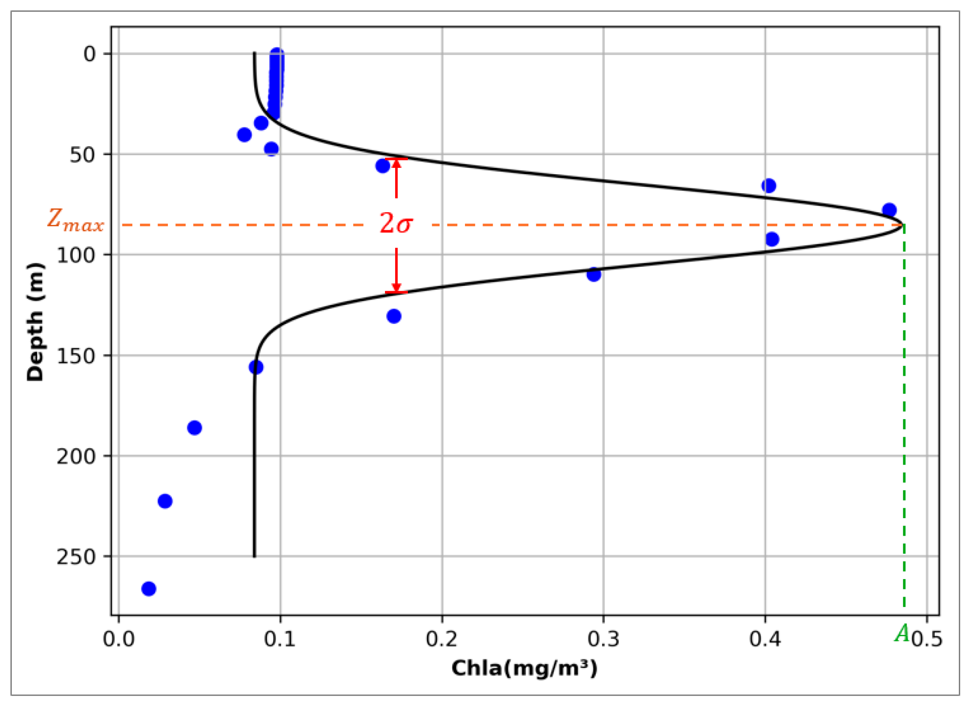
Figure 1. Schematic diagram of Gaussian fitting curve. Each grid profile that meets the SCM determination criteria has the parameters required by the above function extracted accordingly and fitted into a Gaussian curve. The parameters Z m a x , A , 2 σ , in the curve represent the depth intensity and thickness of SCM, respectively.
Remotesensing 17 03283 g001
Figure 2. Taking the data of November 2022 and May 2023 as examples, interpolate the 0.25° data into 1° to correspond to the global grid. (a,b) represent the SCM depth in May and August, respectively, while (c,d) represent the thickness of the pycnocline corresponding to the same time. All those that do not meet the pycnocline and SCM identification criteria are processed with nan values to avoid affecting the average.
Remotesensing 17 03283 g002
Figure 3. Schematic diagram of coupling coefficient calculation. The 26-month global data of SCM and density transition are superimposed. Within each grid, a one-dimensional array of 26 units in length is formed. The arrays in the two datasets are coupled and calculated in pairs. Finally, all the calculation results are extended globally.
Remotesensing 17 03283 g003
Figure 4. (a) shows the global coupling results of SCM and the depth of the maximum change rate of the pycnocline; (b) shows the global coupling results of SCM and the thickness of the pycnocline. And the latitude and longitude range of the specific region: IO (25°N–15°S, 45°E–110°E), NWP (20°N–40°N, 130°E–180°E), SEP (0°S–25°S, 120°W–80°W), NA (5°N–35°N, 70°W–20°W), SA (0°S–25°S, 60°W–0°W).
Remotesensing 17 03283 g004aRemotesensing 17 03283 g004b
Figure 5. Nine-month variations in the pycnocline, SCM, MLD, and ZEU along latitude in the Indian Ocean (25°N–15°S, 45°E–110°E). The three panels in each row represent the three months with the most significant changes within a four-month period. Specifically, the top row corresponds to January–April, the middle row to May–August, and the bottom row to September–December. These nine months are arranged in left-to-right and top-to-bottom order, with the earliest month positioned at the top-left corner and the latest month at the bottom-right corner. The background color represents the rate at which the density changes in depth.
Remotesensing 17 03283 g005
Figure 6. (a) shows the chlorophyll profile. (b) shows the BBP profile. To enhance the contrast between the data, the logarithm base 10 was applied to BBP. (c) illustrates the distribution of BGC-Argo floats in the Indian Ocean region.
Remotesensing 17 03283 g006
Figure 7. The depth variations in the pycnocline, SCM, MLD and ZEU within the nine-month period in the Northwest Pacific (20°N–40°N, 130°E–180°E).
Remotesensing 17 03283 g007
Figure 8. (a) shows the chlorophyll profile. (b) shows the BBP profile. (c) illustrates the distribution of BGC-Argo floats in the Northwest Pacific region.
Remotesensing 17 03283 g008
Figure 9. The depth variations in the pycnocline, SCM, MLD and ZEU within the nine-month period in the Southeast Pacific (0°S–25°S, 120°W–80°W).
Remotesensing 17 03283 g009
Figure 10. (a) shows the chlorophyll profile. (b) shows the BBP profile. (c) illustrates the distribution of BGC-Argo floats in the Southeast Pacific region.
Remotesensing 17 03283 g010
Figure 11. The depth variations in the pycnocline, SCM, MLD and ZEU within the nine-month period in the South Atlantic (0°S–25°S, 60°W–0°W).
Remotesensing 17 03283 g011
Figure 12. (a) shows the chlorophyll profile. (b) shows the BBP profile. (c) illustrates the distribution of BGC-Argo floats in the South Atlantic region.
Remotesensing 17 03283 g012
Table 1. Coupling weights of SCM (depth) and the pycnocline.
Month ω 1 (Thickness) ω 2 (Intensity) ω 3 (Depth) R 2
10.6720.147−0.0850.499
20.6040.24−0.0110.544
30.660.180.0190.587
40.6980.1480.0760.678
50.6320.1230.0750.557
60.6120.0730.0410.452
70.5480.0260.0090.316
80.465−0.0060.0430.243
90.375−0.0030.1890.258
100.334−0.0430.3620.372
110.408−0.0710.3830.478
120.609−0.0750.1630.485
Table 2. Coupling weights of SCM (depth) and the pycnocline.
Month ω 1 (Thickness) ω 2 (Intensity) ω 3 (Depth) R 2
10.3550.2740.2270.567
20.2530.2050.420.573
30.2420.1750.4290.445
40.2390.2330.320.327
50.2860.1960.1990.228
60.4090.1780.0330.228
70.145−0.0080.430.238
80.029−0.2220.4410.317
90.075−0.2450.3210.222
100.354−0.123−0.1490.125
110.3930.123−0.1930.216
120.4740.293−0.1160.436
Table 3. Coupling weights of SCM (depth) and the pycnocline.
Month ω 1 (Thickness) ω 2 (Intensity) ω 3 (Depth) R 2
1−0.124−0.290.0830.117
2−0.323−0.487−0.1350.403
3−0.358−0.4810.0070.446
4−0.329−0.4780.0370.443
5−0.166−0.2190.2760.163
6−0.245−0.413−0.0020.329
7−0.113−0.3650.0820.162
8−0.074−0.3160.1590.099
9−0.174−0.2770.1370.114
10−0.19−0.280.1040.131
11−0.293−0.3190.0110.26
12−0.367−0.393−0.050.434
Table 4. Coupling weights of SCM (depth) and the pycnocline.
Month ω 1 (Thickness) ω 2 (Intensity) ω 3 (Depth) R 2
10.216−0.0750.2290.149
20.232−0.030.3940.323
30.06−0.0280.6460.471
40.008−0.0340.8370.704
50.012−0.0770.8530.728
6−0.023−0.2160.6370.349
70.054−0.2950.3280.112
80.006−0.2410.350.096
90.038−0.1840.2970.07
100.044−0.1640.2660.057
110.141−0.0810.1790.067
120.155−0.0370.2760.14
Disclaimer/Publisher’s Note: The statements, opinions and data contained in all publications are solely those of the individual author(s) and contributor(s) and not of MDPI and/or the editor(s). MDPI and/or the editor(s) disclaim responsibility for any injury to people or property resulting from any ideas, methods, instructions or products referred to in the content.