A Semi-Supervised Multi-Scale Convolutional Neural Network for Hyperspectral Image Classification with Limited Labeled Samples

Highlights

What are the main findings?

• A semi-supervised classification model combining a multi-scale convolutional neural network with a novel pseudo-label strategy ensures high-quality classification of hyperspectral remote sensing images.
• By enhancing the discriminative ability of the classifier through the multi-scale convolutional neural network and improving pseudo-label prediction accuracy via a feature-level augmentation-based pseudo-label generation strategy, the model’s classification performance is elevated.

What is the implication of the main finding?

• This approach enhances the classification performance of hyperspectral remote sensing imagery under conditions of insufficient labelled samples.
• It provides a robust solution to the practical challenge of obtaining labelled samples in real-world applications.

Abstract

Supervised deep learning methods have been widely utilized in hyperspectral image (HSI) classification tasks. However, acquiring a large number of reliably labeled samples to train deep networks is not always possible in practical HSI applications due to the time-consuming and laborious labeling process. Semi-supervised learning is commonly used in scenarios with insufficient labeled samples. However, semi-supervised models based on a pseudo-label strategy often suffer from error accumulation. To address this issue and improve HSI classification performance with few labeled samples, a semi-supervised deep learning approach is proposed. First, a multi-scale convolutional neural network with accurate discriminative capability is constructed to reduce pseudo-label errors. Then, a new pseudo-label generation strategy based on Dropout is presented, in which feature-level data augmentation is applied by considering multiple predictions of the unlabeled samples to mitigate the error accumulation problem. Finally, the multi-scale CNN and the new pseudo-label strategy are integrated into a unified model to improve HSI classification performance. The experimental results demonstrate that the proposed approach outperforms other semi-supervised methods in the literature on four real HSI datasets with limited labeled samples.

1. Introduction

Hyperspectral images (HSIs) contain hundreds of spectral bands that can capture the details of land-cover materials [1,2]. They can be used in a wide range of applications, including environmental monitoring, precision agriculture, mineral exploration, and urban planning [3,4,5,6,7,8]. HSI classification is the most important task in applications of HSI [9].

In recent years, deep learning techniques have achieved great success in HSI classification tasks, where techniques such as the stacked autoencoder (SAE) [10,11], deep belief network (DBN) [12,13], convolutional neural network (CNN) [14,15,16,17,18,19], and recurrent neural network (RNN) [20,21] have been used. These methods do not require manually designed features and achieve excellent classification performance. However, they usually require a large number of labeled samples for the training phase. It is extremely difficult to obtain reliably labeled samples. This sample deficiency can seriously reduce the effectiveness of deep learning-based classification methods in practical applications. Recently, some researchers have attempted to investigate the HSI classification task with insufficient labels [22,23,24,25,26,27]. For example, Duan et al. [26] proposed an innovative framework for oil spill classification and achieved outstanding performance with very limited samples. Xue et al. [27] proposed a spectral–spatial Siamese network (S3Net) for HSI classification in a few-shot training scenario. However, existing methods still have significant room for improvement when facing an extremely limited number of labeled samples. In this study, we aim to alleviate this problem in deep learning techniques to ensure reliable and accurate HSI classification when using a limited number of labeled samples.

Semi-supervised learning is a branch of machine learning in which a model is trained with both labeled samples and unlabeled data to improve model performance under the condition of limited labeled samples. In recent years, semi-supervised learning algorithms based on deep learning have advanced significantly. They can be grouped into five major categories [28], i.e., generative model-based, consistency-regularization-based, graph-based, pseudo-label-based, and hybrid approaches. Deep generative models mainly use generative adversarial networks (GANs) [29] to model data distributions based on unlabeled data. Zhan et al. [30] proposed a GAN-based semi-supervised framework for HSI classification, where the model was only able to utilize spectral information. Zhong et al. [31] combined GANs and Conditional Random Fields (CRFs) for semi-supervised HSI classification. However, GANs are prone to mode collapse. With consistency-regularization-based methods, the model is trained with the assumption that the perturbed samples do not change their labels, so the model finds the smooth manifold of the dataset by exploiting the unlabeled data. Julian et al. [32] introduced Ladder Networks [33] to the semi-supervised HSI classification task with good results. The model explores the information contained in unlabeled data by adding perturbations at the feature level and minimizing the difference between the perturbed and original features. In this approach, two models must be maintained simultaneously during the training process, which increases the demand for hardware devices for model training. Moreover, as explained in detail in Section 2.2, the data augmentation operations often required by such methods are not applicable to HSIs. Graph-based models have also been applied to semi-supervised HSI classification tasks [34,35,36]. However, these methods employ transductive models, which are only able to classify unlabeled samples that are included in the model learning process and thus have poor flexibility and generalization ability, limiting their practical applications. Pseudo-label-based approaches employ strategies for assigning pseudo-labels to unlabeled data and include high-confidence pseudo-labeled samples in the training process. Wu et al. [37] created pseudo-labels by clustering to train a convolutional recurrent neural network for semi-supervised HSI classification. Fang et al. [38] combined pseudo-labeling and co-training for HSI classification. Kang et al. [39] trained a conventional classifier with a small number of labeled samples and selected high-confidence unlabeled samples as pseudo-labeled samples. The hybrid approach combines ideas from the above models to improve performance. Mixmatch [40] and Fixmatch [41] are representative of such models and have achieved impressive performance in natural image classification tasks.

Deep semi-supervised models based on pseudo-labels are widely used for their effectiveness and simplicity [28]. However, semi-supervised pseudo-label-based models may reinforce the errors in a single iteration, resulting in error accumulation, which in turn may mislead the training of subsequent models. Obviously, the direct solution to mitigate the effect of error accumulation is to boost the accuracy of the pseudo-labels; a commonly used strategy to obtain more accurate pseudo-labels is to apply different data augmentation strategies to the unlabeled samples and average the prediction results of different augmented samples. However, due to the characteristics of HSIs, extensive data augmentation may cause spectral distortion. Therefore, this strategy is not applicable to the HSI classification task (see Section 2.2 for more details).

To address these issues, we propose a deep semi-supervised multi-scale CNN model (called MSCNN-D-PL) that combines Dropout and pseudo-labels to improve HSI classification with limited labeled samples. The main contributions of this paper are as follows:

(1)

An MSCNN is presented that contains spatial and spectral multi-scale information extraction modules. Existing convolutional neural network models primarily focus on multi-scale information extraction in the spatial dimension while overlooking the characteristics of hyperspectral data with hundreds of bands in the spectral dimension. In contrast, this study designed a multi-scale feature extraction module with larger convolutional kernels in the spectral dimension. This enhances the model’s receptive field in the spectral dimension, thereby improving its discrimination capability and significantly increasing the accuracy of pseudo-labels predicted for unlabeled samples.

(2)

A new pseudo-label generation strategy based on Dropout [42] is proposed. As a feature-level data augmentation operation, Dropout avoids the problem (which is common in general data augmentation strategies) of changing the spectral response of pixels in HSIs, causing category confusion in spectral response features. Specifically, due to the randomness in Dropout, multiple different classification results for the same unlabeled data can be obtained in multiple Dropout operations. Then, an ensemble learning strategy is adopted to reduce the pseudo-label error by averaging multiple results.

(3)

A deep semi-supervised approach (i.e., MSCNN-D-PL) to HSI classification is proposed. The MSCNN-D-PL achieves more reliable pseudo-labels in deep learning mode for hyperspectral imagery classification. In our experiments on four real HSI datasets with limited labeled samples, it improves the classification accuracy by an average of 4.04% compared to the supervised model and 1.92% compared to other semi-supervised models.

The rest of this paper is organized as follows: The related work and motivation are described in Section 2. In Section 3, the proposed semi-supervised HSI approach is illustrated in detail. Section 4 shows the experimental results and the comparison between the proposed approach and other semi-supervised methods on four HSI datasets. Finally, Section 5 presents the conclusion of the paper.

2. Related Works and Motivation

2.1. CNN for HSI Classification

The CNN, one of the most successful models in image processing, has been widely used in HSI classification tasks [14,15,17,23,43,44,45,46,47,48,49]. Given that an HSI is an image spectrum merging cube data, spatial and spectral information are crucial to achieving better classification performance. Therefore, researchers have designed multiple CNN classification models for extracting spatial–spectral features. For example, a dual-stream framework is used for HSI classification [23,43,44,45], in which one branch extracts spectral information based on a 1D-CNN or SAE, and the other branch extracts spatial information based on a 2D-CNN. The 3D convolution provides a more efficient way to naturally extract spectral–spatial features in HSIs from both spectral and spatial dimensions. Therefore, 3D-CNNs that use 3D cubes as input to integrate all information are widely used in HSI classification [17,46,47]. A continuous learning paradigm that decomposes the 3D-CNN into spectral feature extraction and spatial feature extraction in sequence has been proposed for HSI classification to reduce the number of model parameters and speed up the training process while achieving better generalization performance [48,49]. In addition, advanced deep CNN design patterns, such as residual structure [50] and dense connectivity structure [51], have been widely applied to HSI classification models.

However, capturing multi-scale features of ground objects and extracting complex interactions between hundreds of bands in an HSI remains a difficult problem. For example, the fast dense spectral–spatial convolution network (FDSSC, see Figure 1) [49], which combines a 3D-CNN and densely connected structures, achieves good HSI classification performance. However, the theoretical maxima of the model’s receptive fields are 21 and 99 in the spectral and spatial dimensions, respectively. Thus, considering the hundreds of bands in an HSI, existing models cannot extract interactions between long-distance spectra and cannot adapt to the multi-scale properties of different ground objects in HSIs with varying spatial resolutions. In light of the above problems, we propose a multi-scale CNN (MSCNN) model to effectively extract the spectral–spatial information in HSIs with stronger discriminative power to accurately predict unlabeled samples.

2.2. Semi-Supervised Learning for HSI Classification

The pseudo-label strategy is one of the most widely used semi-supervised classification algorithms, which has the advantage of efficiency in implementation [28]. The most common solution to the error accumulation problem caused by pseudo-labels is to perform augmentation of unlabeled data and average the prediction results of multiple augmentations of each unlabeled data sample to reduce errors in pseudo-labels. Although this strategy has proven effective in natural image classification tasks, it is not applicable to HSIs. Indeed, unlike natural image classification, which assigns a category to each image based on whole-image texture structure information, the HSI classification task is based mainly on the spectral information of the pixels. Consequently, the data augmentation commonly used in natural images will change the spectral response of pixels and potentially cause confusion. To verify the above augmentation issues, a comparative experiment [detailed results in Section 4.3.2] was carried out. The results confirm that standard data augmentation techniques cannot be applied to HSI classification. Therefore, we design a new Dropout-based pseudo-label generation strategy to improve the accuracy and performance of semi-supervised HSI classification.

3. Proposed Approach

In this section, we present the proposed semi-supervised classification approach in detail. It combines a multi-scale convolutional neural network model with a Dropout-based strategy to improve the accuracy of pseudo-labels.

3.1. Multi-Scale CNN Model

3.1.1. Spectral and Spatial Multi-Scale Convolutional Blocks

Inspired by the multi-branch module in GoogLeNet [52], we propose a spectral multi-scale convolutional block (SpecMCB) and a spatial multi-scale convolutional block (SpatMCB), which have large receptive fields and effective spectral–spatial feature extraction capability.

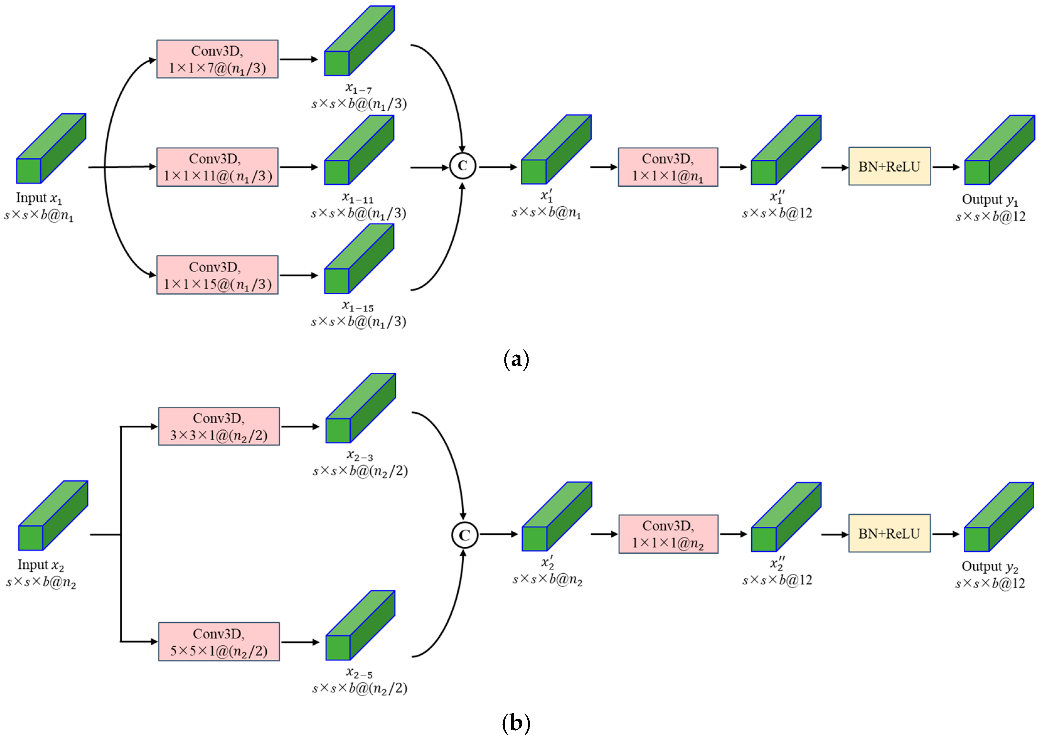
SpecMCB is shown in Figure 2a. It contains three parallel convolutional layers with kernel sizes 1 × 1 × 7, 1 × 1 × 11, and 1 × 1 × 15 to extract multi-scale spectral features. The stride size is (1, 1, 1), and the corresponding padding operation is performed according to the convolutional kernel size to maintain a constant feature map size after convolutional processing. The input of SpecMCB is assumed to be $x_1$, characterized by $n_1$ feature maps with a size of s × s × b, where s × s is the spatial size of one feature map and b is the number of spectral bands. Then, $x_{1-7}$, $x_{1-11}$, and $x_{1-15}$ (all with $n_1/3$ feature maps with a size of s × s × b) are obtained after the three above-described convolutional layers. Afterward, $x_{1-7}$, $x_{1-11}$, and $x_{1-15}$ are concatenated to obtain $x_1^{\prime }$, characterized by $n_1$ feature maps (the C operation in Figure 2a). Finally, $x_1^{\prime }$ is fused using 1 × 1 × 1 convolution to obtain the feature map $x_1^{″}$, which contains the multi-scale information. To ensure stable training of the model and increase its nonlinear feature extraction capability, batch normalization (BN) [53] and nonlinear activation layers are applied to the end of SpecMCB to process $x_1^{″}$. The final multi-scale spectral feature $y_1$ is obtained, where the nonlinear activation function adopted is the rectified linear unit (ReLU) [54].

For spatial information extraction, we designed the spatial multi-scale convolution block (SpatMCB) (Figure 2b) in a similar way to the spectral block. However, given the relatively small spatial size of the input samples in HSI classification, the designed SpatMCB contains only two parallel convolutional layers of different kernel sizes, 3 × 3 × 1 and 5 × 5 × 1, with the same stride size (1, 1, 1). The corresponding padding operation is performed according to the size of the convolutional kernel so that the size of the feature map after the convolution process remains unchanged. Let ${\mathrm{x}}_2$, with ${\mathrm{n}}_2$ feature maps with a size of s × s × b, be the input of SpatMCB. Then, $x_{2-3}$ and ${\mathrm{x}}_{2-5}$ with ${\mathrm{n}}_2/2$ feature maps with a size of s × s × b are obtained after the above-described two convolution layers. Afterwards, ${\mathrm{x}}_2^{\prime }$, characterized by ${\mathrm{n}}_2$ feature maps, is obtained by concatenation between ${\mathrm{x}}_{2-3}$ and ${\mathrm{x}}_{2-5}$. Here, the 1 × 1 × 1 convolution is again adopted to fuse the $x_2^{\prime }$ and obtain a multi-scale feature map $x_2^{″}$. Finally, the BN layer and the ReLU activation layer, which enable stable training of the model and increase the nonlinear feature extraction capability of SpatMCB, are used to process ${\mathrm{x}}_2^{″}$ to obtain the final multi-scale spatial feature $y_2$.

3.1.2. Overview of the Proposed Classification Model

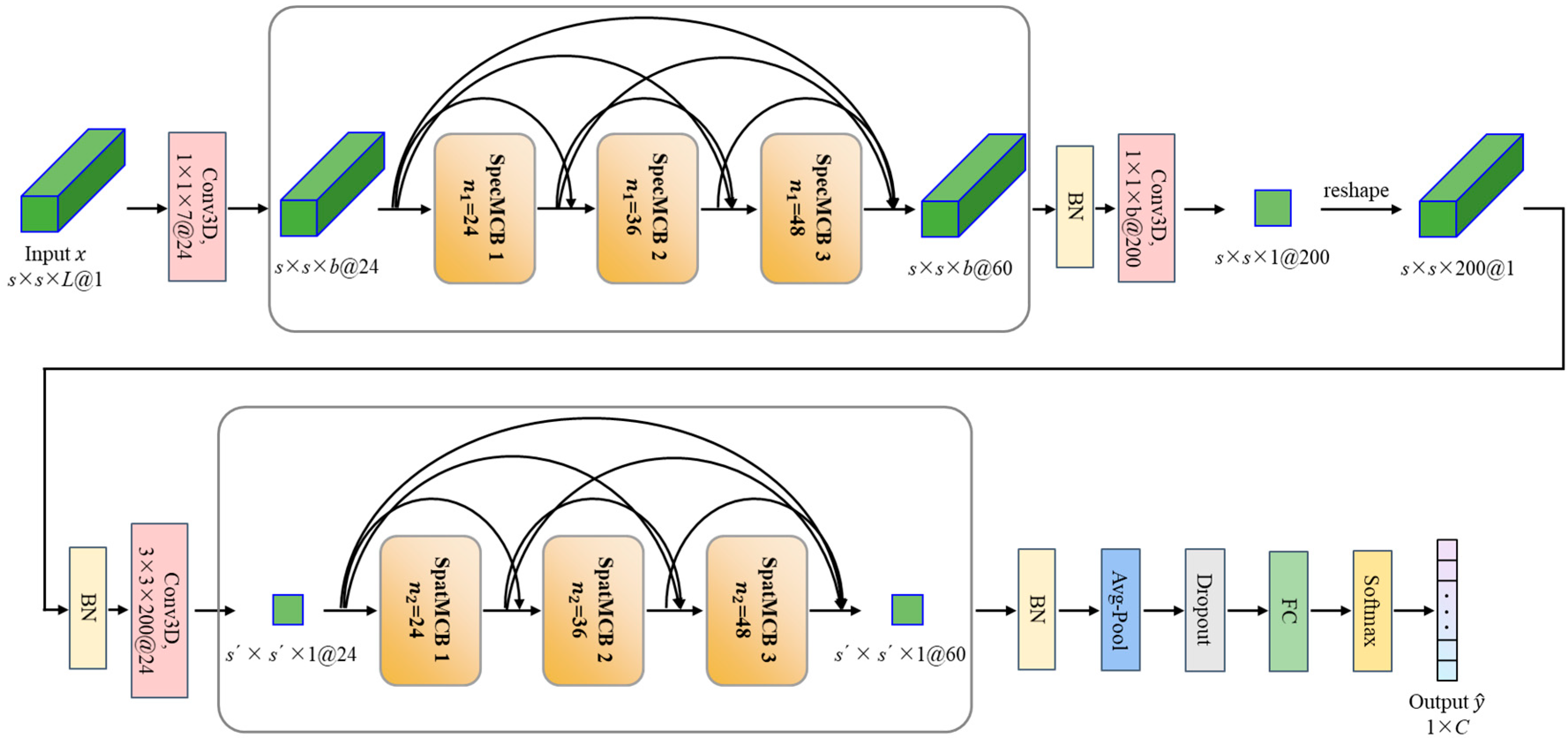
In this subsection, we introduce a multi-scale CNN (MSCNN) model (see Figure 3) that combines SpecMCB and SpatMCB. The architecture details of the proposed MSCNN are given in

Table 1. Architecture details of the proposed MSCNN (taking the Indian Pines dataset as an example).

Module		Input Size	Layer Type	Padding	Output Size
Conv3D		(1, 9, 9, 200)	Conv3D (kernelsize = 1 × 1 × 7, stride = 1 × 1 × 2, dim = 24,)	N	(24, 9, 9, 97)
Spectral multi-scale information extraction module	SpecMCB1	(24, 9, 9, 97)	Parallel {Conv3D (kernelsize = 1 × 1 × 7, dim = 8), Conv3D (kernelsize = 1 × 1 × 11, dim = 8), Conv3D (kernelsize = 1 × 1 × 15, dim = 8)}, Concat, Conv3D (kernelsize = 1 × 1 × 1, dim = 12), BN, ReLU	Y	(12, 9, 9, 97)
	SpecMCB2	(36, 9, 9, 97)	Parallel {Conv3D (kernelsize = 1 × 1 × 7, dim = 12), Conv3D (kernelsize = 1 × 1 × 11, dim = 12), Conv3D (kernelsize = 1 × 1 × 15, dim = 12)}, Concat, Conv3D (kernelsize = 1 × 1 × 1, dim = 12), BN, ReLU	Y	(12, 9, 9, 97)
	SpecMCB3	(48, 9, 9, 97)	Parallel {Conv3D (kernelsize = 1 × 1 × 7, dim = 16), Conv3D (kernelsize = 1 × 1 × 11, dim = 16), Conv3D (kernelsize = 1 × 1 × 15, dim = 16)}, Concat, Conv3D (kernelsize = 1 × 1 × 1, dim = 12), BN, ReLU	Y	(12, 9, 9, 97)
Conv3D		(60, 9, 9, 97)	BN, Conv3D (kernelsize = 1 × 1 × 97, dim = 200)	N	(200, 9, 9, 1)
Permute		(200, 9, 9, 1)	-	-	(1, 9, 9, 200)
Conv3D		(1, 9, 9, 200)	BN, ReLU, Conv3D (kernelsize = 3 × 3 × 200, dim = 24)	N	(24, 7, 7, 1)
Spatial multi-scale information extraction module	SpatMCB1	(24, 7, 7, 1)	Parallel {Conv3D (kernelsize = 3 × 3 × 1, dim = 12), Conv3D (kernelsize = 5 × 5 × 1, dim = 12)}, Concat, Conv3D (kernelsize = 1 × 1 × 1, dim = 12), BN, ReLU	Y	(12, 7, 7, 1)
	SpatMCB2	(36, 7, 7, 1)	Parallel {Conv3D (kernelsize = 3 × 3 × 1, dim = 18), Conv3D (kernelsize = 5 × 5 × 1, dim = 18)}, Concat, Conv3D (kernelsize = 1 × 1 × 1, dim = 12), BN, ReLU	Y	(12, 7, 7, 1)
	SpatMCB3	(48, 7, 7, 1)	Parallel {Conv3D (kernelsize = 3 × 3 × 1, dim = 24), Conv3D (kernelsize = 5 × 5 × 1, dim = 24)}, Concat, Conv3D (kernelsize = 1 × 1 × 1, dim = 12), BN, ReLU	Y	(12, 7, 7, 1)
Avg-Pool		(60, 7, 7, 1)	GlobalAvgPooling, Flatten	-	(60)
Dropout		(60,)	Dropout	-	(60)
FC		(60,)	Fully Connected	-	(16)

. The MSCNN has a larger receptive field with higher discriminative ability to improve the accuracy of predicted pseudo-labels for unlabeled samples.

The input $x$ of the MSCNN is a 3D cube with a size of s × s × L, where s is the size of $x$ in the spatial dimension, and L denotes the number of bands of $x$. The first convolutional layer, containing 24 convolution kernels with a kernel size of 1 × 1 × 7, a stride size of (1, 1, 2), and no padding, is applied to $x$, resulting in 24 feature maps with a size of s × s × b, where $\mathrm{b}=⌊\left(L-7\right)/2+1⌋$, $⌊·⌋$ is the floor function. After that, a spectral multi-scale information extraction module (shown in the upper part of Figure 3), which contains three sequentially connected SpecMCBs and a dense connection structure, is used to extract the spectral multi-scale information. The densely connected structure adopted here can alleviate the vanishing gradient phenomenon and prevent overfitting. Due to the dense connectivity structure and the fact that each SpecMCB can extract 12 multi-scale spectral features with a size of s × s × b, the spectral multi-scale information extraction module finally extracts 60 multi-scale features having a size of s × s × b.

To facilitate spatial multi-scale information extraction, the 60 features are first processed by BN. Then, a 1 × 1 × b convolution layer is adopted to obtain 200 feature maps with a size of s × s × 1. Subsequently, the 200 feature maps with a size of s × s × 1 are reshaped into 1 feature map with a size of s × s × 200. Finally, the feature map is processed by BN, the ReLU activation function, and a 3D convolutional layer with 24 convolutional kernels of size 3 × 3 × 200 to obtain 24 feature maps of size $s^{\prime }$ × $s^{\prime }$ × 1 for spatial information extraction.

The spatial multi-scale information extraction module has a similar structure to its spectral counterpart. Note that the inputs to the spatial multi-scale information extraction module are the features extracted by the spectral multi-scale information extraction module. As a result, the features extracted by each SpatMCB contain multi-scale spatial–spectral information. Because a dense connection structure is used, the spatial multi-scale information extraction module can extract 60 multi-scale spatial–spectral features with a size of $s^{\prime }$ × $s^{\prime }$ × 1.

Finally, the extracted multi-scale spatial–spectral features are sequentially processed by a global average pooling layer (GAP), Dropout, and a fully connected (FC) layer. The softmax layer is used to generate a 1 × C vector indicating the probability that the sample belongs to each category, where C denotes the number of classes of the corresponding dataset. The proposed MSCNN model assembled with multi-scale information extraction modules (i.e., SpecMCB and SpatMCB) has a larger receptive field and is able to extract richer multi-scale features, resulting in better classification performance. As a result, the pseudo-labeled samples derived from this model contain fewer errors than those obtained with other techniques, which mitigates the error accumulation problem faced by pseudo-label-based semi-supervised learning.

3.2. Dropout-Based Pseudo-Label Generation Strategy

In the previous subsection, we introduced an MSCNN model to mitigate errors in pseudo-labels of unlabeled data. In this part, we present a new pseudo-label generation strategy based on Dropout to further enhance the precision of pseudo-labels and thus improve the performance of semi-supervised HSI classification. Dropout [42] is a common and effective regularization technique for alleviating overfitting in deep learning. It is considered a type of implicit feature-level data augmentation [55,56], in which the process of randomly dropping neural units can generate different features from the same sample. Given that the data augmentation techniques generally used for natural images change the spectral response of the pixels, to avoid spectral distortion, they should not be applied to HSIs. Therefore, in this subsection, we propose a Dropout-based pseudo-label generation strategy to address this issue.

The MSCNN model is first trained with $N_1$ epochs based on a small number of labeled samples. Then, the MSCNN with Dropout activated is used to predict the labels of unlabeled data. Due to the presence of the Dropout layer in the MSCNN model, different classification probability vectors are obtained by performing multiple predictions on the same unlabeled sample. Then, the multiple classification probability vectors for the same unlabeled sample can be averaged to obtain a more accurate classification probability vector for it. Finally, the high-confidence and accurate pseudo-labeled data are selected and appended to the training set to train a better classification model.

Suppose that ${\mathrm{x}}_{\mathrm{u}}$ denotes an unlabeled sample, ${\mathrm{f}}_{\mathrm{u}}$ is its feature vector obtained after the Dropout layer in the MSCNN model, and $P_u=\left\{p\left(y_u=j|x_u\right)\right\}, j=\mathrm{1,2},\cdots ,C$, obtained after the FC and softmax layers, indicates the probability vector that ${\mathrm{x}}_{\mathrm{u}}$ belongs to each of the C classes. Thus, if an unlabeled sample ${\mathrm{x}}_{\mathrm{u}}$ is predicted K times independently, K different feature representations $\left\{{\mathrm{f}}_{\mathrm{u}}^1,{\mathrm{f}}_{\mathrm{u}}^2,\cdots ,{\mathrm{f}}_{\mathrm{u}}^{\mathrm{K}}\right\}$ will be obtained, which in turn will result in K probability vectors $\left\{{\mathrm{P}}_{\mathrm{u}}^1,{\mathrm{P}}_{\mathrm{u}}^2,\cdots ,{\mathrm{P}}_{\mathrm{u}}^{\mathrm{K}}\right\}$ of ${\mathrm{x}}_{\mathrm{u}}$. The final probability vector $\overline{{\mathrm{P}}_{\mathrm{u}}}=\left\{\overline{\mathrm{p}}\left({\mathrm{y}}_{\mathrm{u}}=\mathrm{j}|{\mathrm{x}}_{\mathrm{u}}\right)\right\}, j=\mathrm{1,2},\cdots ,C$ of ${\mathrm{x}}_{\mathrm{u}}$ is obtained by averaging the K predicted results according to (1).

$\overline{{\mathrm{P}}_{\mathrm{u}}}$ can better reflect the category information of the unlabeled sample ${\mathrm{x}}_{\mathrm{u}}$. After obtaining the classification probability vector $\overline{{\mathrm{P}}_{\mathrm{u}}}$ for all unlabeled data, those with classification confidence higher than a threshold $p_t$ (a predefined probability threshold indicating the likelihood that a sample belongs to a specific class) are selected and added to the training set to train the classification model again. The MSCNN model is trained again with ${\mathrm{N}}_2$ epochs based on the updated training set to further improve the classification performance. This process can be repeated several times until a stopping condition is satisfied, e.g., when a preset number of epochs is reached.

$$\overline{p}\left(y_u=j|x_u\right)={\displaystyle \frac{1}{K}}{\sum }_{k=1}^K{p}^k\left(y_u=j|x_u\right)$$

(1)

3.3. Multi-Scale CNN Combining Dropout and Pseudo-Labels

Combining the designed MSCNN classification model and the Dropout-based pseudo-label generation strategy, a semi-supervised multi-scale convolutional neural network classification model, i.e., the MSCNN-D-PL, is obtained. The detailed procedure is illustrated in Algorithm 1.

Algorithm 1: MSCNN-D-PL

Input:

$\mathrm{Hyperspectral} \mathrm{image} \mathrm{dataset}, X=\left\{x_1\right.,x_2,\cdots ,x_i,\cdots ,\left.x_N\right\}$   $\mathrm{Labeled} \mathrm{sample} \mathrm{set}, {\left\{X_L,Y_L\right\}}_{i=1}^L$  $\mathrm{Unlabeled} \mathrm{sample} \mathrm{set}, {\left\{X_U\right\}}_{i=1}^U$  $\mathrm{Test} \mathrm{sample} \mathrm{set}, {\left\{X_T,Y_T\right\}}_{i=1}^T$ Number of unlabeled samples’ predictions, K $\mathrm{Threshold} \mathrm{value} \mathrm{adapted} \mathrm{for} \mathrm{selecting} \mathrm{high}-\mathrm{confidence} \mathrm{unlabeled} \mathrm{samples}, p_t$ Total number of epochs, N Number of epochs for training MSCNN at first, N1 Number of epochs for training MSCNN with the updated labeled sample set, N2

Output:

$\mathrm{Predicted} \mathrm{labels} \mathrm{of} \mathrm{test} \mathrm{samples}, Y_T$

Procedure:

1. $\mathrm{Training} \mathrm{MSCNN} \mathrm{with} N_1 \mathrm{epochs} \mathrm{on} \left\{X_L,Y_L\right\}$. 2. $\mathrm{Predicting} \mathrm{the} \mathrm{unlabeled} \mathrm{samples} X_U$$K \mathrm{times} \mathrm{with} \mathrm{MSCNN}, \mathrm{obtaining} \mathrm{the} \mathrm{class} \mathrm{probabilities} \left\{P_u^1, P_u^2,\cdots ,P_u^K\right\}$. 3. $\mathrm{Calculating} \mathrm{the} \mathrm{mean} \mathrm{class} \mathrm{probabilities} \overline{P_u}$$\mathrm{of} X_U$ with Equation (1). 4. $\mathrm{Selecting} \mathrm{the} \mathrm{high}-\mathrm{confidence} \mathrm{unlabeled} \mathrm{sample} \mathrm{set} X_U^{\prime }$$\mathrm{with} Y_U^{\prime }$$\mathrm{based} \mathrm{on} p_t$. 5. $\mathrm{Updating} \mathrm{the} \mathrm{labeled} \mathrm{sample} \mathrm{set} X_L:=X_L\cup X_U^{\prime }$$, Y_L:=Y_L\cup Y_U^{\prime }$$; \mathrm{updating} \mathrm{the} \mathrm{unlabeled} \mathrm{sample} \mathrm{set} X_U:=X_U-X_U^{\prime }$. 6. $\mathrm{Retraining} \mathrm{MSCNN} \mathrm{with} N_2 \mathrm{epochs} \mathrm{on} \left\{X_L,Y_L\right\}$. 7. $\mathrm{Repeating} \mathrm{steps} 2–6 \mathrm{until} \mathrm{the} \max \mathrm{number} \mathrm{of} \mathrm{epochs} N \mathrm{is} \mathrm{reached} \mathrm{or} \mathrm{there} \mathrm{are} \mathrm{no} \mathrm{high}-\mathrm{confidence} \mathrm{unlabeled} \mathrm{samples} \mathrm{to} \mathrm{be} \mathrm{selected} \mathrm{based} \mathrm{on} p_t$. $\mathrm{Predicting} \mathrm{the} \mathrm{label} Y_T$$\mathrm{of} \mathrm{test} \mathrm{samples} X_T$ with the latest MSCNN model.

4. Experimental Results and Discussion

In this section, the results of extensive experiments conducted on four widely used hyperspectral benchmark datasets are presented to verify the validity of the proposed MSCNN-D-PL. All experiments were performed on a PC workstation with Pytorch (v2.0) [57] running on an Intel (R) Core (TM) i7-5930K 3.50 GHz CPU with 32 GB RAM and an NVIDIA GeForce RTX 3090 Graphics Processing Unit.

4.1. Description of Datasets

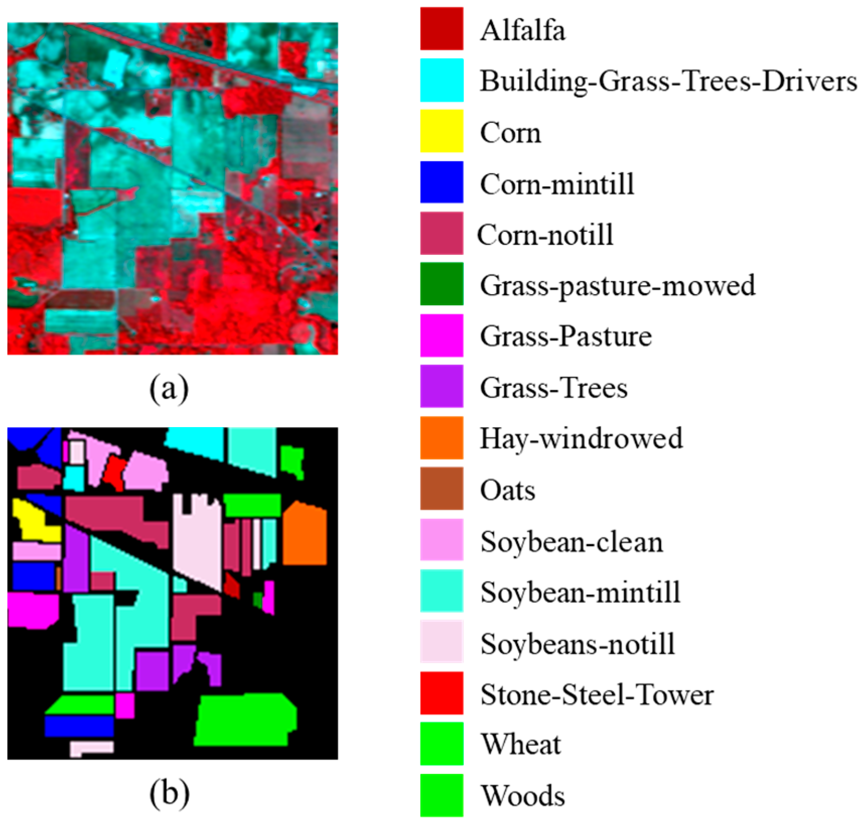
(1) Indian Pines: This dataset was collected in 1992 by the Airborne Visible/Infrared Imaging Spectrometer sensor (AVIRIS) (NASA’s Jet Propulsion Laboratory, Pasadena, CA, USA) from the Indian Pines Test Site in northwestern Indiana (USA). The Indian Pines dataset consists of 145 × 145 pixels with a relatively low spatial resolution of 20 m/pixel and a spectral resolution of 10 nm, covering a wavelength range of 400–2500 nm and containing 224 bands. The 24 water absorption and noise bands around 1400~1900 nm were removed, and 200 bands were included in the experiment. The dataset contains 16 different types of land cover, with a total of 10,249 labeled samples. Figure 4 shows the false-color composition of the dataset and the ground-truth map.

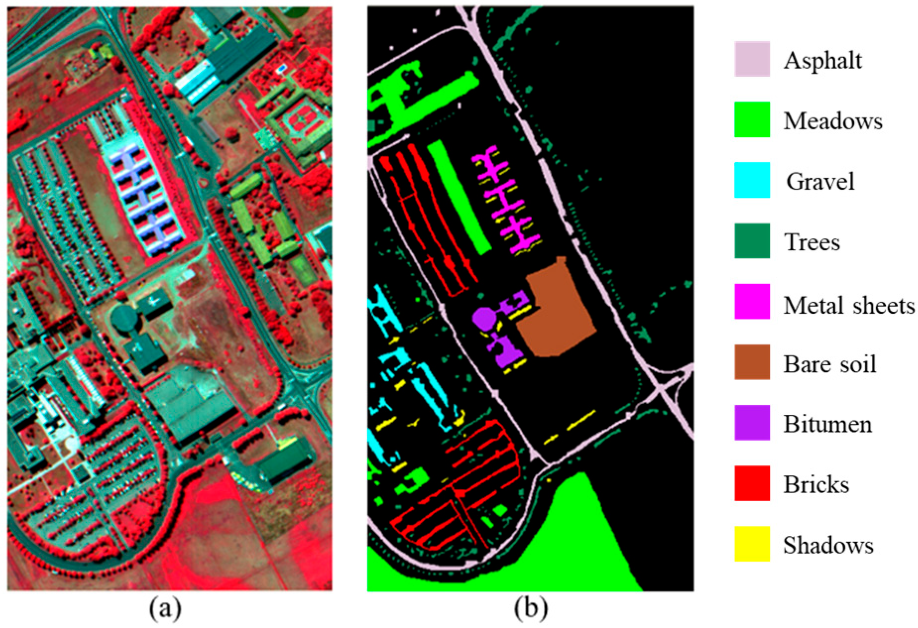
(2) Pavia University: The second dataset represents an urban scene. It was collected at the University of Pavia, Italy, in 2002 with the Reflective Optics System Imaging Spectrometer System (ROSIS). These data consist of 115 spectral bands covering the wavelength range 430–860 nm and contain 610 × 340 pixels with a spatial resolution of 1.3 m/pixel. After removing 12 noise bands, the dataset used for the experiments contains 103 spectral bands. The dataset contains a total of 42,776 labeled samples covering nine types of ground objects. Figure 5 displays the false-color composition image and the corresponding ground-truth map of this dataset.

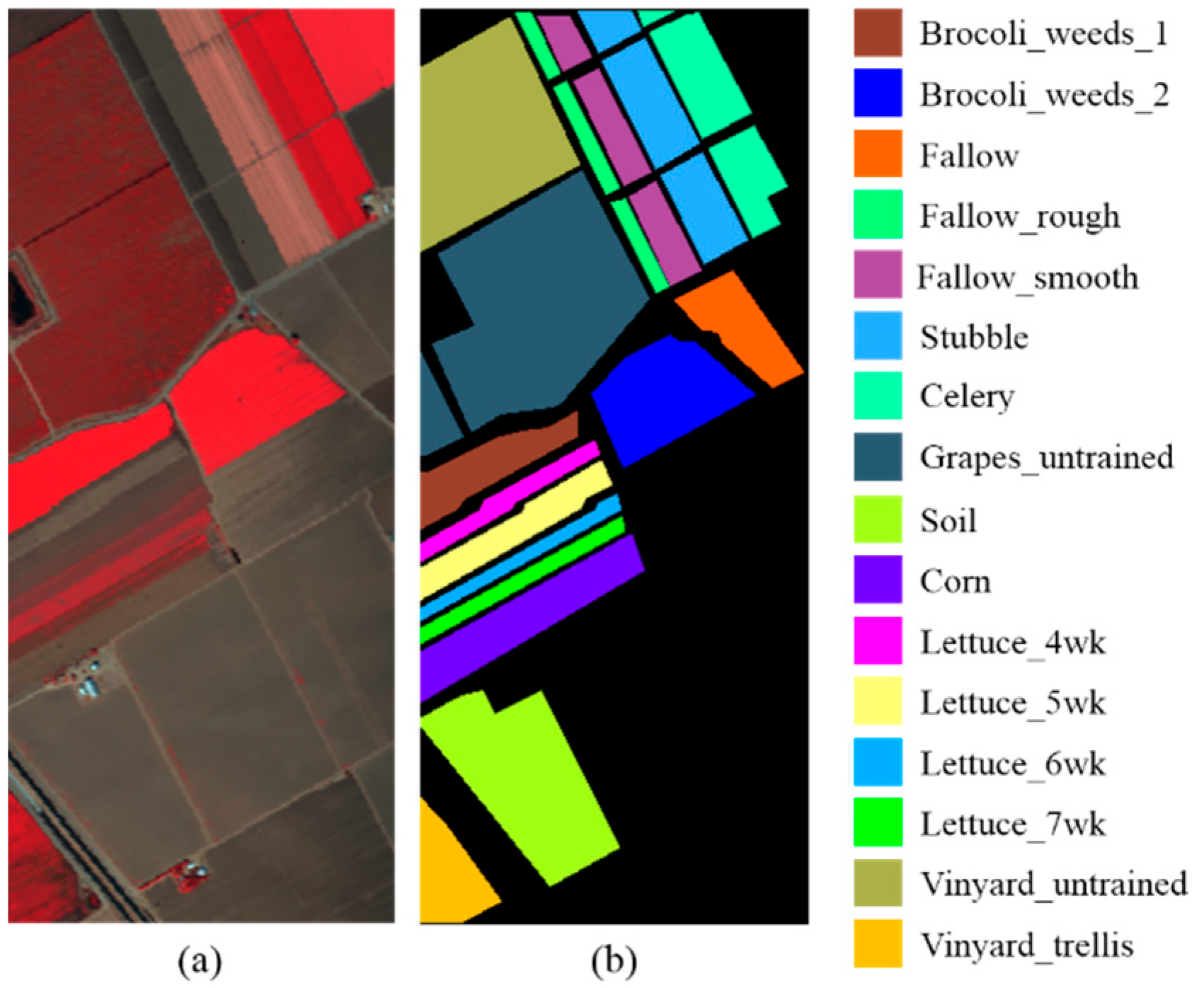
(3) Salinas Valley: The Salinas Valley dataset was acquired with the same AVIRIS sensor as the Indian Pines dataset. It was taken at the Salinas Valley in California. The spatial size of the Salinas Valley image is 512 × 217 pixels, with a high spatial resolution of 3.7 m/pixel. The data consisted of 224 bands, 20 of which were not usable for experiments due to the influence of water absorption. The majority of the land cover types in this dataset are crops, which have a relatively regular distribution. There are 54,129 labeled samples distributed among 16 different types of ground objects. The false-color image composition and reference land-cover map are shown in Figure 6.

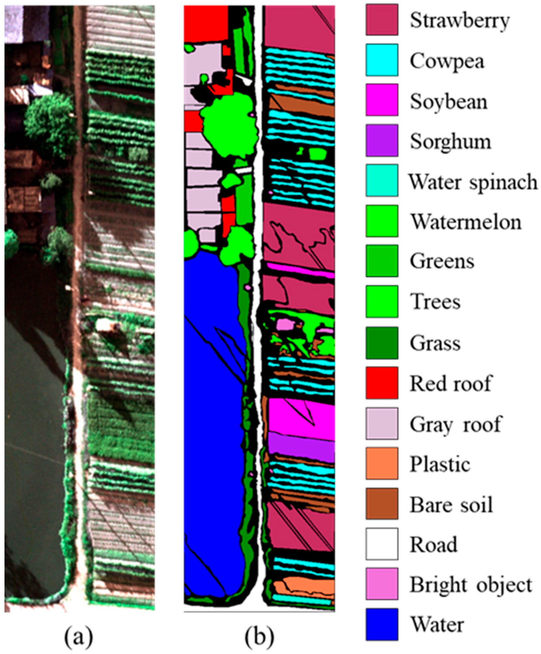
(4) WHU-Hi-HanChuan [58,59]: This dataset was collected on 17 June 2016, in Hanchuan City, Hubei Province, China, by the Headwall Nano-Hyperspec imaging sensor on a Leica Aibot X6 UAV V1 platform. The UAV-borne hyperspectral image consists of 1217 × 303 pixels with a very high spatial resolution of 0.109 m/pixel and an average spectral resolution of 2.22 nm, containing 270 bands covering a wavelength range of 400–1000 nm. The study area has a complex agricultural landscape with a wide variety of crops. The dataset consists of 257,530 labeled samples containing 16 landform types. The false-color composition image and the corresponding ground-truth map are shown in Figure 7.

4.2. Experimental Settings

To thoroughly evaluate the effectiveness of the proposed MSCNN-D-PL, several state-of-the-art semi-supervised methods, i.e., DSR-GCN [60], 3D-GAN [30], PseudoLabel [37], MeanTeacher [61], MixMatch [40], and FixMatch [41], were chosen as comparison benchmarks. These comparison methods are briefly described as follows:

(1)

DSR-GCN [60]: A transductive semi-supervised classification model based on a differentiated-scale restricted graph convolutional network.

(2)

3D-GAN [30]: A semi-supervised classification model based on a generative adversarial network (GAN), in which both the generator and discriminator are 3D CNNs.

(3)

PseudoLabel [37]: A semi-supervised classification model based on a traditional pseudo-label strategy.

(4)

MeanTeacher [61]: A semi-supervised classification model based on consistent regularization.

(5)

MixMatch [40]: A deep semi-supervised classification model based on a hybrid strategy combining pseudo-labels and consistent regularization.

(6)

FixMatch [41]: A deep semi-supervised classification model based on a hybrid strategy combining pseudo-labels and consistent regularization and achieving impressive performance in the field of natural image classification.

It should be emphasized that the MSCNN is also adopted as a benchmark classifier for the PseudoLabel, MeanTeacher, MixMatch, and FixMatch methods. The results of the MSCNN are also reported for comparison in the experiments.

Semi-supervised learning is commonly used in scenarios with insufficient label information. Thus, a limited number of labeled samples were included in the training sets in the following experiments. For the Indian Pines dataset, we randomly selected, from each class, 1% of samples for the training set and 50% of samples for the unlabeled dataset, with the rest used as the test set. The Pavia University, Salinas Valley, and WHU-Hi-HanChuan datasets have more labeled samples than the Indian Pines dataset. Therefore, for the three datasets, for each class, 0.1% of samples were randomly selected for the training set, 5% of samples for the unlabeled dataset, and the remaining samples for the test set. More details of the number of labeled samples for each class are listed in

Table 2. Land-cover classes and the related number of training samples (Indian Pines dataset).

Dataset	Label	Class	Total Samples	Training Samples
Indian Pines	1	Alfalfa	54	1
	2	Bldg-Grass-Trees-Drivers	380	4
	3	Corn	234	2
	4	Corn-mintill	834	8
	5	Corn-notill	1434	14
	6	Grass-pasture-mowed	26	1
	7	Grass-Pasture	497	5
	8	Grass-Trees	747	7
	9	Hay-windrowed	489	5
	10	Oats	20	1
	11	Soybean-clean	614	6
	12	Soybean-mintill	2468	25
	13	Soybean-notill	968	10
	14	Stone-Steel-Tower	95	1
	15	Wheat	212	2
	16	Woods	1294	13
	Total		10,366	105

,

Table 3. Land-cover classes and the related number of training samples (Pavia University dataset).

Dataset	Label	Class	Total Samples	Training Samples
Pavia University	1	Asphalt	6631	7
	2	Meadows	18,649	19
	3	Gravel	2099	2
	4	Trees	3064	3
	5	Metal sheets	1345	1
	6	Bare soil	5029	5
	7	Bitumen	1330	1
	8	Bricks	3682	4
	9	Shadows	947	1
	Total		42,776	43

,

Table 4. Land-cover classes and the related number of training samples (Salinas Valley dataset).

Dataset	Label	Class	Total Samples	Training Samples
Salinas Valley	1	Brocoli_weeds_1	2009	2
	2	Brocoli_weeds_2	3726	4
	3	Fallow	1976	2
	4	Fallow_rough	1394	1
	5	Fallow_smooth	2678	3
	6	Stubble	3959	4
	7	Celery	3579	4
	8	Grapes_unstrained	11,271	11
	9	Soil	6203	6
	10	Corn	3278	3
	11	Lettuce_4wk	1068	1
	12	Lettuce_5wk	1927	2
	13	Lettuce_6wk	916	1
	14	Lettuce_7wk	1070	1
	15	Vinyard_unstrained	7268	7
	16	Vinyard_trellis	1807	2
	Total		54,129	54

and

Table 5. Land-cover classes and the related number of training samples (WHU-Hi-HanChuan dataset).

Dataset	Label	Class	Total Samples	Training Samples
WHU-Hi-HanChuan	1	Strawberry	44,735	45
	2	Cowpea	22,753	23
	3	Soybean	10,287	10
	4	Sorghum	5353	5
	5	Water spinach	1200	1
	6	Watermelon	4533	5
	7	Greens	5903	6
	8	Trees	17,978	18
	9	Grass	9469	9
	10	Red roof	10,516	11
	11	Gray roof	16,911	17
	12	Plastic	3679	4
	13	Bare soil	9116	9
	14	Road	18,560	19
	15	Bright object	1136	1
	16	Water	75,401	75

. The Adam [62] optimizer and cross-entropy loss function were adopted for all methods during model training, with the learning rate set to 0.001, the batch size set to 32, and the number of epochs set to 150. For the MSCNN-D-PL model, in all experiments, the parameters N₁ and N₂ were set to 80 and 10, respectively. Thus, we first trained the MSCNN with 80 epochs based on the initial training set. Then, in the subsequent semi-supervised process, the training set was updated according to the Dropout-based pseudo-label generation strategy. After that, the MSCNN was trained for 10 epochs on the updated training set using the previous training settings. The optimal model was finally obtained by repeating this semi-supervised process iteratively.

Three common metrics used to evaluate the accuracy of models are Producer’s accuracy, overall accuracy, and the Kappa coefficient. (1) Producer’s accuracy (PA): For a given class, PA is the probability that a reference sample of that class was correctly classified. It measures the model’s ability to correctly predict a specific class on the ground. A low PA for “Class i” means that many “Class i” areas were missed (errors of omission). (2) Overall accuracy (OA): OA, the most straightforward metric, represents the proportion of all test samples that were classified correctly. It gives a general, aggregate view of the model’s performance. However, it can be misleading if the class distribution is imbalanced, as it may be skewed by high accuracy for the majority class. (3) Kappa coefficient (Kappa): A more robust statistic that measures the agreement between the classification and the reference data while accounting for the agreement expected by random chance. It answers the question “How much better is my classification than a random assignment of labels?” A value of 1 indicates perfect agreement, 0 indicates agreement equal to chance, and negative values indicate performance worse than chance. The Kappa coefficient is often considered a more reliable measure than OA, especially for imbalanced datasets. Due to the small number of labeled samples, 10 independent experiments were conducted to reduce the effect of the randomness of sample selection on the classification results. The means and standard deviations of the results are reported.

4.3. Results

In this subsection, the results of exhaustive experiments are presented to show the properties and the effectiveness of the proposed MSCNN-D-PL. In the following experiments, we first validate the effectiveness of the designed MSCNN model. Then, we assess the impact of data augmentation on HSI classification. Finally, we compare the results of the proposed MSCNN-D-PL with those of other semi-supervised methods on the four considered HSI datasets.

4.3.1. MSCNN Results

In Section 3.1, we pointed out that the designed MSCNN model has a larger receptive field and can capture multi-scale information to obtain higher classification accuracy. Here, in addition to FDSSC, three representative supervised HSI classification methods, i.e., A-SPN [25], S3Net [27], and SPRLT-Net [63], were selected as benchmarks to fully illustrate the effectiveness of the MSCNN in the case of insufficient labeled samples. The A-SPN and S3Net are designed for the HSI classification task with limited labeled samples, while SPRLT-Net is a transformer-based model capable of representing the global receptive field.

The results obtained using the experimental setup in Section 4.2 are reported in

Table 6. Classification performance on the four considered datasets.

Methods	Indian Pines		Pavia University		Salinas Valley		WHU-Hi-HanChuan
	OA (%)	Kappa (%)	OA (%)	OA (%)	OA (%)	Kappa (%)	OA (%)	Kappa (%)
A-SPN	84.77 ± 1.43	82.51 ± 1.67	74.46 ± 2.74	64.01 ± 4.37	77.65 ± 4.37	74.51 ± 5.08	82.16 ± 1.63	78.63 ± 2.01
S3Net	75.93 ± 2.17	72.68 ± 2.53	80.54 ± 2.67	74.08 ± 3.19	86.84 ± 1.58	85.37 ± 1.73	80.82 ± 2.96	77.42 ± 3.48
SPRLT-Net	57.40 ± 2.57	49.58 ± 3.41	68.47 ± 1.34	54.62 ± 2.52	60.35 ± 5.07	54.67 ± 5.97	72.63 ± 1.74	67.35 ± 2.17
FDSSC	86.07 ± 2.41	84.04 ± 2.48	87.21 ± 1.71	82.62 ± 2.08	89.03 ± 1.68	87.77 ± 1.69	84.61 ± 1.83	81.85 ± 2.23
MSCNN	89.26 ± 1.21	87.77 ± 1.26	89.81 ± 1.47	85.91 ± 1.89	91.41 ± 1.81	90.37 ± 1.82	86.24 ± 0.98	83.83 ± 1.15

. As can be seen, the designed MSCNN model achieves the best classification accuracy on all four datasets, with OA improvements of 3.19%, 2.60%, 2.38%, and 1.63%, respectively, compared to the suboptimal FDSSC model. SPRLT-Net exhibits the worst performance, possibly because transformer-based models tend to have low accuracy when trained on insufficient training samples, although they have global modeling capabilities.

Similar conclusions can be obtained from the Kappa coefficient. This indicates that the MSCNN can extract more discriminative features and thus has better classification performance. The results also show that the MSCNN exhibits higher stability on the Indian Pines, Pavia University, and WHU-Hi-HanChuan datasets. Thus, the designed MSCNN model is more suitable as a base classifier for semi-supervised classification models due to its higher classification accuracy and its ability to reduce errors in pseudo-labels.

4.3.2. Impact of Data Augmentation on HSI Classification

In Section 2.2, we intuitively and qualitatively analyzed the reasons that the data augmentation strategies used in natural image classification are not applicable to HSI classification. To quantitatively assess the impact of data augmentation on HSI classification, three data augmentation strategies with different strengths were adopted. The first test does not use augmentation operations during model training (denoted as NoAug); the second test only performs random horizontal or vertical flip augmentation (denoted as Aug+), which does not change the spectral values of pixels; and the third uses RandAugment [64], commonly used in natural image tasks (denoted as Aug++). RandAugment consists of 14 common augmentation operations, as shown in

Table 7. Detailed information on the RandAugment strategy.

ID	Augmentation Operations	Changing the Spectral Value or Not	Adopted or Not
1	AutoContrast	√	√
2	Brightness	√	√
3	Color	√	√
4	Contrast	√	√
5	Equalize	√	×
6	Identity	×	√
7	Posterize	√	×
8	Rotate	×	√
9	Sharpness	√	√
10	ShearX	×	√
11	ShearY	×	√
12	Solarize	√	√
13	TranslateX	×	√
14	TranslateY	×	√

. As one can see from the table, eight augmentation operations change the spectral values of pixels. Two augmentation operations (i.e., Equalize and Posterize) are discarded because they can only handle RGB images, thus leaving only 12 augmentation operations in Aug++.

Table 8. Classification performance of the MSCNN and FDSSC with different data augmentation strategies on the four considered datasets.

Dataset		Indian Pines		Pavia University		Salinas Valley		WHU-Hi-HanChuan
Model		FDSSC	MSCNN	FDSSC	MSCNN	FDSSC	FDSSC	MSCNN	FDSSC
Augmentation Type	NoAug	86.07 ± 2.41	89.26 ± 1.21	87.21 ± 1.71	89.81 ± 1.47	89.03 ± 1.68	91.41 ± 1.81	84.61 ± 1.83	86.24 ± 0.98
	Aug+	85.95 ± 1.86	89.40 ± 1.07	87.36 ± 1.47	89.72 ± 1.23	89.11 ± 1.43	91.33 ± 1.52	84.26 ± 1.43	86.15 ± 0.82
	Aug++	82.15 ± 3.66	86.18 ± 2.35	82.01 ± 3.85	85.73 ± 1.96	85.64 ± 3.19	89.26 ± 2.18	81.57 ± 2.69	83.72 ± 1.87

shows the results obtained with different strengths on the four datasets, using the same experimental setup as in the previous subsection.

It is clear from Table 8 that the classification accuracy of the FDSSC and MSCNN models with Aug++ is significantly decreased on all four datasets compared to the results of NoAug. In addition, the stability of the model trained with Aug++ is poor. It can also be observed that the classification accuracy of the model trained with Aug+ data augmentation is close to that of NoAug. This may be because remote sensing images are generally captured from an overhead view, which makes the ground objects in the images isotropic, and horizontal or vertical flip data augmentation cannot provide additional information. As a result, the models with Aug+ achieve almost the same classification accuracy as those with NoAug. The results confirm that common data augmentation strategies used for natural images are not applicable to HSIs.

4.3.3. Comparison with State-of-the-Art Methods

In this subsection, the proposed MSCNN-D-PL is compared with six state-of-the-art semi-supervised methods and one supervised model, i.e., MSCNN. It should be noted that the MeanTeacher and MixMatch methods require weak data augmentation for unlabeled data, as implemented with Aug+ in Section 4.3.2. The FixMatch method requires both strong and weak data augmentation for unlabeled data. Thus, the Aug++ and Aug+ data augmentation strategies described in Section 4.3.2 were used.

(1) Experimental results on the Indian Pines dataset

The classification accuracies of the proposed MSCNN-D-PL and the comparison methods on the Indian Pines dataset are shown in

Table 9. Quantitative assessment of classification results on the Indian Pines dataset.

Accuracy Metric	Label	Methods
		MSCNN	DSR-GCN	3D-GAN	PseudoLabel	MeanTeacher	MixMatch	FixMatch	MSCNN-D-PL
PA (%)	1	77.86 ± 4.79	83.58 ± 19.06	50.49 ± 9.16	76.94 ± 4.56	75.15 ± 3.09	75.14 ± 6.53	73.23 ± 2.42	82.83 ± 2.38
	2	71.52 ± 2.23	87.67 ± 8.47	51.56 ± 4.36	70.72 ± 1.81	70.64 ± 1.26	71.89 ± 2.49	68.06 ± 1.91	80.84 ± 1.67
	3	76.32 ± 2.47	79.87 ± 8.88	55.53 ± 3.05	74.55 ± 2.29	73.95 ± 2.94	77.07 ± 2.63	69.70 ± 4.29	80.07 ± 2.57
	4	79.80 ± 1.83	83.32 ± 8.99	67.14 ± 2.88	80.44 ± 1.66	79.65 ± 1.50	80.86 ± 1.29	78.05 ± 1.14	85.55 ± 1.15
	5	85.64 ± 0.84	86.21 ± 5.20	77.29 ± 0.76	85.50 ± 0.76	84.98 ± 0.80	86.61 ± 1.05	84.24 ± 1.09	89.69 ± 0.86
	6	85.06 ± 5.39	100.00 ± 0.00	65.35 ± 12.96	85.66 ± 5.93	83.82 ± 8.33	89.38 ± 5.39	86.01 ± 5.51	90.21 ± 3.80
	7	94.17 ± 1.26	79.72 ± 11.12	90.63 ± 1.81	94.81 ± 0.90	94.63 ± 1.37	96.07 ± 0.91	93.78 ± 0.62	96.25 ± 0.85
	8	97.85 ± 0.56	95.95 ± 1.90	96.54 ± 1.50	98.11 ± 0.62	97.56 ± 0.56	98.07 ± 0.76	97.72 ± 1.03	98.50 ± 0.39
	9	98.34 ± 0.45	98.64 ± 2.23	98.81 ± 0.57	98.75 ± 0.35	98.91 ± 0.41	98.90 ± 0.50	98.81 ± 0.37	99.16 ± 0.32
	10	74.30 ± 9.88	79.47 ± 27.60	53.05 ± 7.79	75.91 ± 6.33	74.45 ± 11.57	80.22 ± 10.00	69.55 ± 10.10	89.09 ± 5.57
	11	82.65 ± 2.19	77.06 ± 18.17	68.52 ± 3.63	84.20 ± 1.51	83.64 ± 1.29	85.75 ± 1.49	82.51 ± 2.37	90.30 ± 1.50
	12	91.07 ± 0.84	90.57 ± 7.28	85.77 ± 1.14	91.84 ± 0.42	91.21 ± 0.83	91.59 ± 0.41	90.70 ± 0.82	93.90 ± 0.44
	13	87.31 ± 1.04	79.00 ± 5.75	79.85 ± 1.89	87.69 ± 1.16	87.99 ± 0.96	88.73 ± 1.59	87.23 ± 1.36	91.40 ± 0.69
	14	87.69 ± 1.76	92.98 ± 10.36	83.48 ± 4.66	87.85 ± 1.87	87.84 ± 1.13	88.93 ± 2.77	87.66 ± 1.74	90.62 ± 3.28
	15	98.81 ± 0.67	96.90 ± 2.32	96.29 ± 2.47	98.80 ± 0.47	99.04 ± 0.69	98.59 ± 0.79	98.54 ± 0.74	99.31 ± 0.51
	16	97.11 ± 0.53	96.24 ± 8.63	95.75 ± 1.31	97.20 ± 0.35	97.09 ± 0.59	97.17 ± 0.72	97.07 ± 0.54	97.66 ± 0.28
OA (%)		89.26 ± 1.21	88.23 ± 3.72	82.35 ± 1.49	89.61 ± 1.33	89.24 ± 1.61	90.10 ± 1.47	88.50 ± 2.23	92.57 ± 0.79
Kappa (%)		87.77 ± 1.26	86.62 ± 4.14	79.76 ± 1.56	88.13 ± 1.53	87.82 ± 1.65	88.67 ± 1.50	86.86 ± 2.30	91.52 ± 0.92

. As one can see from the table, the proposed MSCNN-D-PL achieves the highest classification accuracy. The OA and Kappa coefficient of the MSCNN-D-PL are improved by 3.31% and 3.75%, respectively, compared to the MSCNN model without the semi-supervised strategy, and by 2.47% and 2.85%, respectively, compared to the MixMatch method, which achieves suboptimal performance on this dataset. Furthermore, one can observe that the MSCNN-D-PL has better classification accuracy in each category compared to all comparison methods except the DSR-GCN. In particular, for relatively overlapping categories, such as the Otas (label 10) and Building-Grass-Trees-Drivers (label 2), the classification accuracy of the proposed MSCNN-D-PL improved by 8.95% and 8.87%, respectively, over the suboptimal results obtained by MixMatch.

Table 9 shows that the MixMatch method obtained the second-best classification results. However, its classification accuracy is not significantly better than that of the supervised MSCNN. The PseudoLabel method ranks third in classification accuracy. It is slightly better than the MSCNN, which indicates that the semi-supervised model based on the traditional pseudo-label strategy cannot fully exploit the information contained in unlabeled data. MeanTeacher, which only uses the consistent regularization semi-supervised strategy, and the FixMatch method, which combines both pseudo-label and consistent regularization semi-supervised strategies, did not achieve satisfactory results. The 3D-GAN semi-supervised method based on the generative adversarial network provided the worst classification result, possibly because the training process for 3D-GAN requires a large number of labeled samples. The DSR-GCN model also fails to achieve better classification results. This may be due to the limited number of training samples, as well as the lower spatial resolution of this dataset, decreasing the model’s discriminative ability.

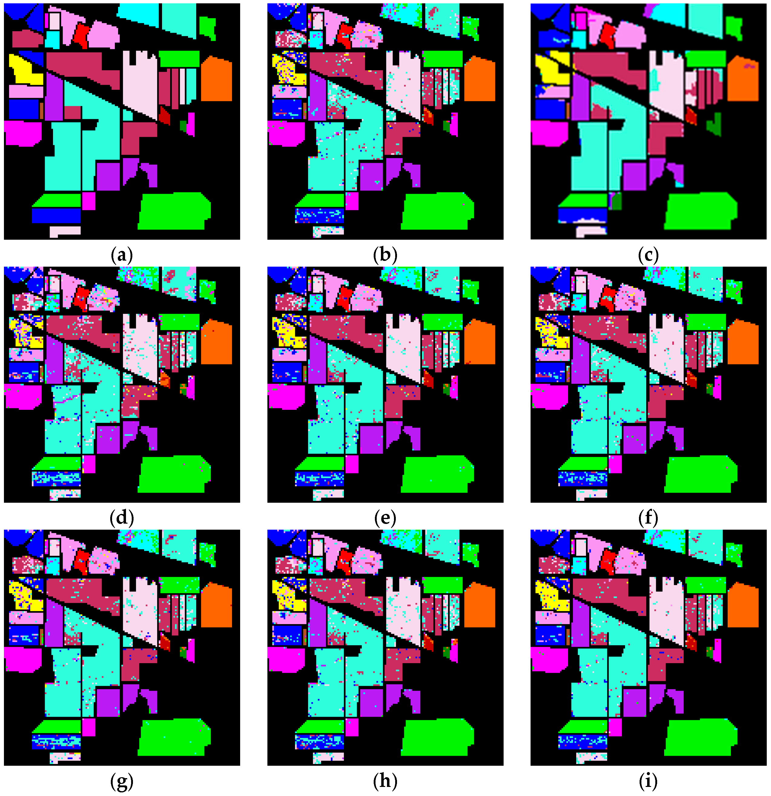
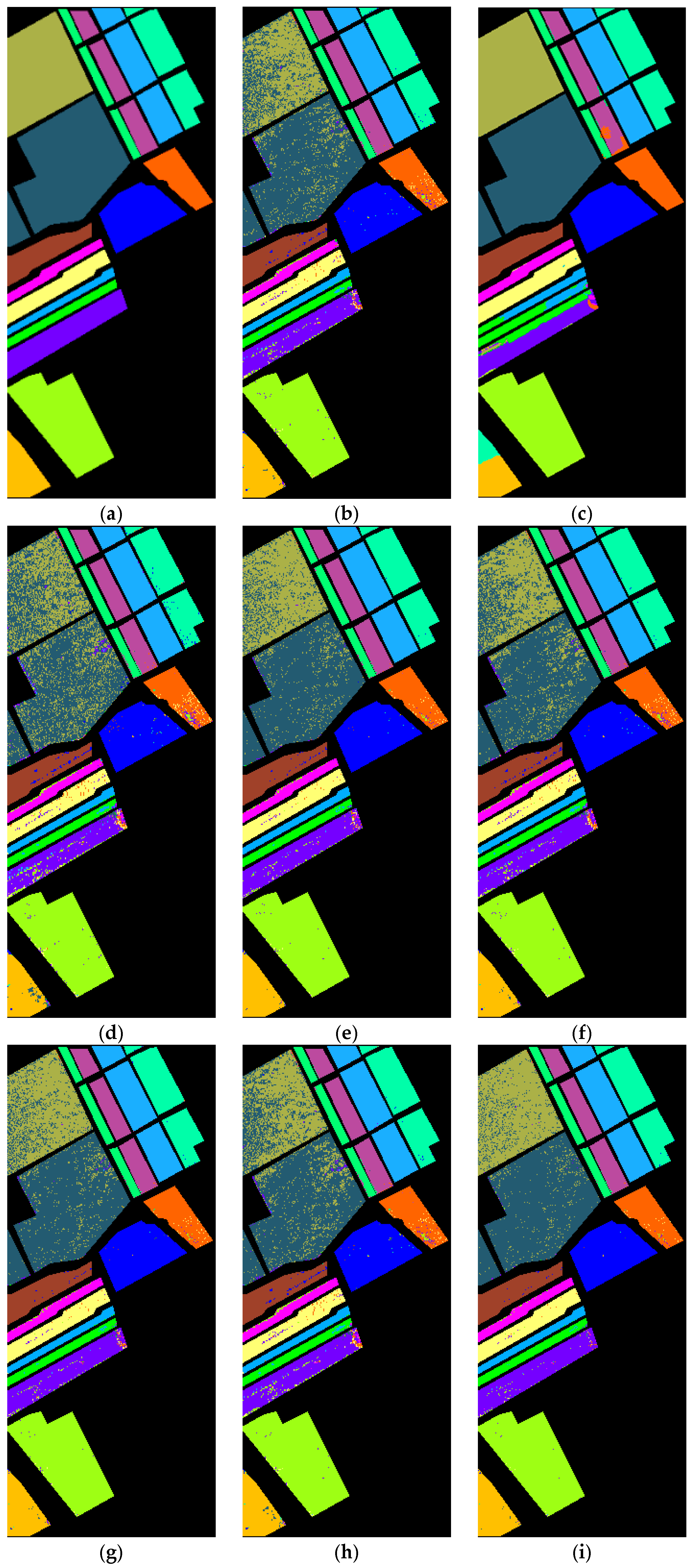
Figure 8 shows the classification maps obtained by each method. One can see that the proposed MSCNN-D-PL model (Figure 8i) has smoother classification results and fewer cases of misclassification compared to other methods.

(2) Experimental results on the Pavia University dataset

Table 10. Quantitative assessment of classification results on the Pavia University dataset.

Accuracy Metric	Label	Methods
		MSCNN	DSR-GCN	3D-GAN	PseudoLabel	MeanTeacher	MixMatch	FixMatch	MSCNN-D-PL
PA (%)	1	87.81 ± 2.33	91.43 ± 7.38	84.23 ± 2.69	90.69 ± 0.91	88.43 ± 3.70	92.41 ± 0.65	87.94 ± 1.79	94.00 ± 0.29
	2	98.22 ± 0.44	95.85 ± 4.75	95.95 ± 1.62	98.66 ± 0.15	97.81 ± 0.61	98.79 ± 0.14	97.77 ± 0.75	99.10 ± 0.08
	3	64.93 ± 5.87	68.38 ± 21.18	55.48 ± 11.54	69.49 ± 3.62	59.06 ± 7.21	73.31 ± 1.99	58.25 ± 6.27	78.41 ± 1.15
	4	89.40 ± 2.73	65.39 ± 17.45	80.57 ± 6.87	92.16 ± 1.39	89.44 ± 1.05	94.54 ± 0.63	87.77 ± 2.33	96.03 ± 0.32
	5	97.66 ± 1.27	99.53 ± 1.01	87.52 ± 12.22	98.61 ± 0.45	97.14 ± 3.16	99.22 ± 0.40	96.89 ± 5.04	99.43 ± 0.06
	6	72.88 ± 4.79	95.90 ± 6.56	62.38 ± 10.51	82.37 ± 1.33	73.77 ± 3.28	86.09 ± 1.20	72.73 ± 3.52	88.96 ± 0.69
	7	58.01 ± 11.37	83.43 ± 25.94	51.60 ± 14.02	66.86 ± 4.19	55.88 ± 11.93	73.03 ± 2.71	57.22 ± 7.37	81.61 ± 1.18
	8	88.80 ± 2.35	90.75 ± 10.18	83.76 ± 4.09	88.12 ± 1.97	87.68 ± 3.35	90.33 ± 1.41	87.45 ± 3.16	91.99 ± 0.50
	9	99.73 ± 0.15	50.94 ± 16.04	99.44 ± 0.29	99.79 ± 0.14	99.66 ± 0.14	99.85 ± 0.13	99.83 ± 0.08	99.84 ± 0.12
OA (%)		89.81 ± 1.47	89.94 ± 2.37	84.50 ± 1.33	91.82 ± 1.49	89.30 ± 1.53	93.23 ± 1.39	88.88 ± 1.86	94.75 ± 1.93
Kappa (%)		85.91 ± 1.89	86.65 ± 3.00	78.86 ± 1.84	89.19 ± 1.96	85.31 ± 1.92	90.97 ± 1.46	84.76 ± 2.12	93.03 ± 2.55

shows the classification accuracies of the proposed MSCNN-D-PL and comparison methods on the Pavia University dataset. It is observed that the proposed MSCNN-D-PL obtains the best classification accuracy and has high stability. The MixMatch model achieves the second-best classification accuracy. The supervised MSCNN model achieves an OA and Kappa coefficient of 89.81% and 85.91, respectively, which outperforms the partially semi-supervised models. The OA and Kappa coefficient of the MSCNN-D-PL are improved by 1.52% and 2.06% over MixMatch and 4.94% and 7.12% over the MSCNN, respectively. Moreover, it can be observed that the proposed MSCNN-D-PL achieves the best classification accuracy for almost all categories compared to other methods. In particular, for two classes, i.e., Gravel (label 3) and Bitumen (label 7), which are the most difficult to classify in this dataset, the proposed MSCNN-D-PL obtained high classification accuracies, equal to 78.41 ± 1.15% and 81.61 ± 1.18%, respectively. From Table 10, we can also observe that the PseudoLabel method yields the third-best classification accuracy, with 2% improvement over the MSCNN model. The DSR-GCN method achieves slightly better classification accuracy than the supervised MSCNN, i.e., 89.94% vs. 89.81%. The MeanTeacher method still does not produce good results on this dataset. The FixMatch method with strong Aug++ data augmentation also performed poorly, with lower classification accuracy than the supervised MSCNN method. The 3D-GAN yields the worst classification results, with an OA 5.31% lower than that of the MSCNN.

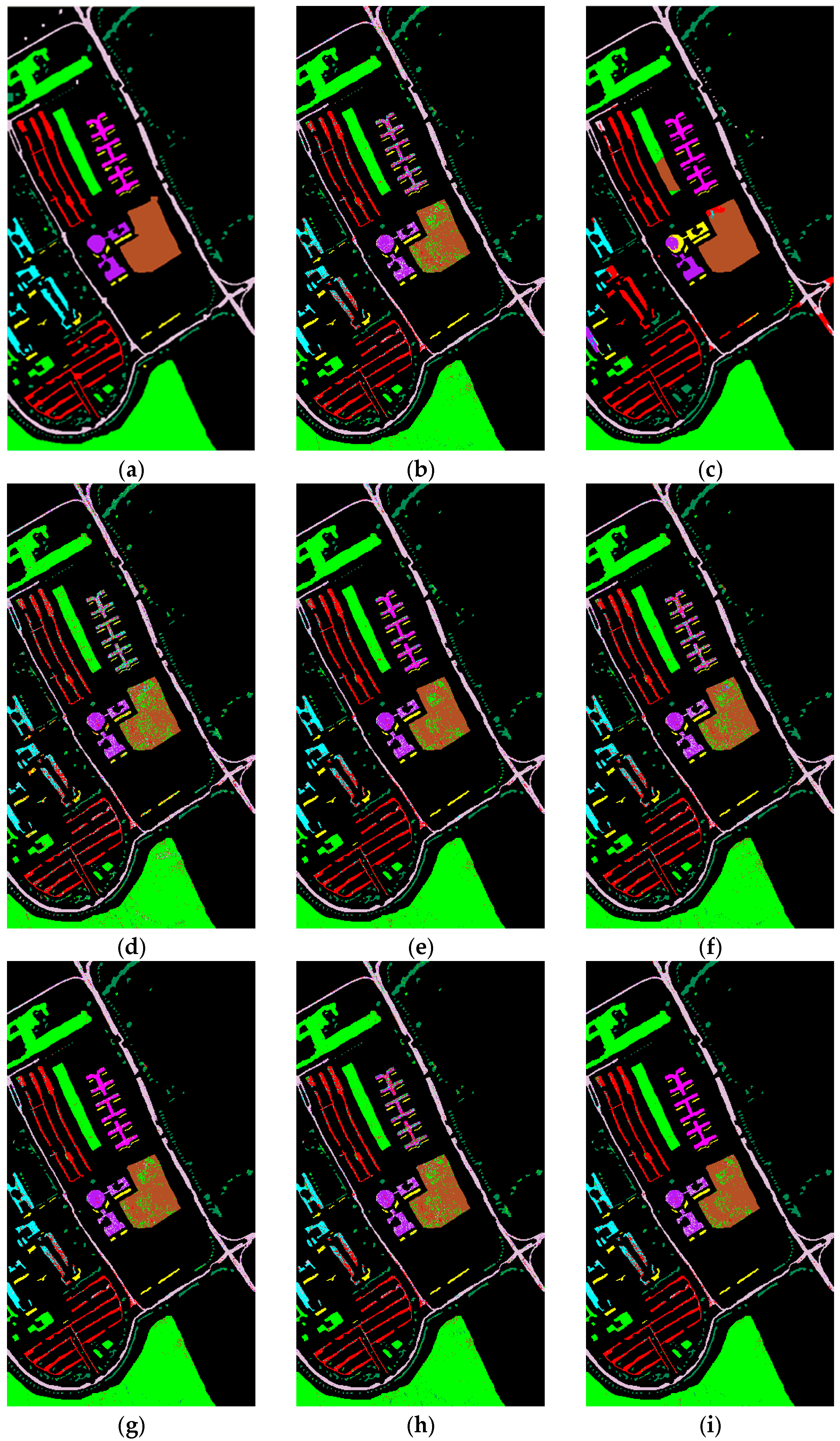
To facilitate a visual comparison of the classification performance of each model, Figure 9 shows maps of the classification results of all methods. One can see that the classification map of the proposed MSCNN-D-PL (Figure 9i) has fewer misclassifications.

(3) Experimental results on the Salinas Valley dataset

The experimental results obtained by all methods on the Salinas Valley dataset are shown in

Table 11. Quantitative assessment of classification results on the Salinas Valley dataset.

Accuracy Metric	Label	Methods
		MSCNN	DSR-GCN	3D-GAN	PseudoLabel	MeanTeacher	MixMatch	FixMatch	MSCNN-D-PL
PA (%)	1	97.12 ± 2.14	100.00 ± 0.00	94.22 ± 4.25	98.26 ± 1.28	97.13 ± 2.11	98.27 ± 1.52	96.80 ± 2.26	98.97 ± 1.11
	2	99.36 ± 1.85	100.00 ± 0.00	97.99 ± 3.00	99.61 ± 0.95	99.27 ± 1.74	99.58 ± 1.17	99.20 ± 2.00	99.74 ± 0.97
	3	94.40 ± 2.27	90.12 ± 15.84	86.70 ± 7.71	96.37 ± 1.42	93.64 ± 2.11	96.58 ± 1.64	93.82 ± 2.63	97.80 ± 1.13
	4	98.21 ± 1.99	82.20 ± 21.04	96.68 ± 3.53	98.90 ± 1.25	98.08 ± 2.01	98.95 ± 1.33	97.90 ± 2.40	99.18 ± 1.12
	5	98.71 ± 1.89	94.01 ± 5.22	98.31 ± 2.58	99.16 ± 1.07	98.68 ± 1.73	99.23 ± 1.28	98.63 ± 2.07	99.36 ± 1.02
	6	99.67 ± 1.84	99.58 ± 0.28	99.45 ± 2.50	99.81 ± 0.94	99.72 ± 1.72	99.77 ± 1.16	99.53 ± 2.01	99.86 ± 0.95
	7	99.47 ± 1.85	99.93 ± 0.09	98.68 ± 2.75	99.62 ± 0.99	99.52 ± 1.75	99.62 ± 1.21	99.32 ± 2.04	99.82 ± 0.98
	8	88.17 ± 2.31	96.37 ± 3.49	74.03 ± 4.79	92.62 ± 1.42	86.49 ± 1.99	92.67 ± 1.63	86.49 ± 2.44	95.05 ± 1.44
	9	99.13 ± 1.77	100.00 ± 0.00	99.01 ± 2.64	99.44 ± 0.97	99.15 ± 1.65	99.40 ± 1.16	98.97 ± 1.98	99.63 ± 0.96
	10	89.96 ± 2.09	88.40 ± 12.18	80.07 ± 5.73	93.38 ± 1.53	88.51 ± 2.20	93.50 ± 1.70	88.74 ± 2.60	95.62 ± 1.51
	11	90.24 ± 2.46	99.39 ± 0.56	87.91 ± 3.47	93.71 ± 1.48	90.09 ± 2.34	93.56 ± 1.61	89.76 ± 2.72	95.81 ± 1.78
	12	96.38 ± 1.97	90.59 ± 13.95	92.87 ± 3.66	97.89 ± 1.18	96.07 ± 1.82	97.71 ± 1.41	95.87 ± 2.20	98.42 ± 1.12
	13	98.13 ± 2.03	81.01 ± 16.10	98.06 ± 2.80	98.91 ± 1.27	98.20 ± 1.94	98.80 ± 1.35	97.97 ± 2.17	99.30 ± 1.08
	14	94.44 ± 2.12	78.97 ± 21.72	91.21 ± 3.95	96.45 ± 1.28	93.81 ± 2.36	96.53 ± 1.57	94.22 ± 2.44	97.67 ± 1.26
	15	67.30 ± 2.28	96.43 ± 3.95	56.55 ± 4.82	78.63 ± 2.33	64.91 ± 2.24	79.07 ± 2.65	64.22 ± 2.25	85.58 ± 2.12
	16	97.52 ± 2.14	90.37 ± 10.30	91.87 ± 4.98	98.81 ± 1.08	97.29 ± 2.33	98.68 ± 1.22	97.29 ± 2.31	99.21 ± 1.07
OA (%)		91.41 ± 1.81	95.50 ± 1.85	85.33 ± 2.76	94.46 ± 1.28	90.55 ± 1.74	94.53 ± 1.49	90.40 ± 2.02	96.29 ± 1.15
Kappa (%)		90.37 ± 1.82	95.00 ± 2.06	83.62 ± 2.71	93.84 ± 1.43	89.44 ± 1.76	93.91 ± 1.54	89.29 ± 2.04	95.87 ± 1.28

and Figure 10. As one can see from Table 11, the proposed MSCNN-D-PL achieves the best classification performance in terms of the OA and Kappa coefficient, i.e., 96.29% and 95.87%, respectively. The supervised MSCNN also achieves good results, with an OA of 91.41%, and still performs better than the three compared semi-supervised methods, i.e., the 3D-GAN, FixMatch, and MeanTeacher. Moreover, compared to the supervised MSCNN model, the OA and Kappa coefficient are improved by 4.88% and 5.50%, respectively. The transductive DSR-GCN model obtains suboptimal performance on this dataset and achieves 100% classification accuracy for 3 of the 16 categories. The inductive MixMatch method also achieves satisfactory classification results on this dataset. When examining the classification accuracy for each class (PA), the results show that the MSCNN-D-PL improves the classification accuracy for all classes compared to all comparison methods except the DSR-GCN. For Vinyard_unstrained (label 15), the MSCNN-D-PL improves the classification accuracy with respect to MixMatch from 79.07% to 85.58%. The standard deviation from experiments shows that the MSCNN-D-PL approach has higher stability for most categories. The PseudoLabel model achieves the fourth-best classification performance on this dataset, slightly below MixMatch, with an improvement of 3% compared to the supervised MSCNN method.

(4) Experimental results on the WHU-Hi-HanChuan dataset

Table 12. Quantitative assessment of classification results on the WHU-Hi-HanChuan dataset.

Accuracy Metric	Label	Methods
		MSCNN	DSR-GCN	3D-GAN	PseudoLabel	MeanTeacher	MixMatch	FixMatch	MSCNN-D-PL
PA (%)	1	97.16 ± 0.12	97.61 ± 1.68	95.89 ± 1.13	97.90 ± 0.06	97.49 ± 0.05	98.07 ± 0.06	96.91 ± 0.09	98.23 ± 0.11
	2	84.45 ± 1.39	85.88 ± 3.41	77.05 ± 1.15	88.15 ± 1.34	85.49 ± 1.25	89.13 ± 1.24	82.74 ± 1.23	90.20 ± 0.71
	3	74.63 ± 1.66	87.87 ± 6.52	67.96 ± 1.67	79.72 ± 1.40	76.10 ± 1.35	81.75 ± 1.35	71.63 ± 1.66	83.54 ± 1.18
	4	96.33 ± 0.22	94.20 ± 2.21	94.09 ± 1.33	97.09 ± 0.15	96.56 ± 0.36	97.28 ± 0.20	95.89 ± 0.26	97.72 ± 0.17
	5	18.17 ± 1.33	37.61 ± 21.62	5.67 ± 1.42	35.92 ± 1.48	22.85 ± 1.78	40.67 ± 1.33	11.20 ± 2.37	46.28 ± 1.13
	6	22.05 ± 2.56	70.37 ± 14.73	12.07 ± 2.47	39.11 ± 1.43	26.18 ± 1.68	43.25 ± 1.33	15.85 ± 2.59	48.90 ± 1.36
	7	86.46 ± 1.65	87.56 ± 13.10	81.52 ± 1.30	89.17 ± 0.54	86.86 ± 1.33	89.65 ± 1.47	84.31 ± 1.47	90.91 ± 1.32
	8	81.85 ± 1.40	83.65 ± 5.07	74.53 ± 1.88	86.35 ± 1.22	83.06 ± 1.37	86.95 ± 1.11	79.97 ± 1.46	88.38 ± 1.28
	9	69.38 ± 2.63	74.03 ± 5.01	57.50 ± 2.23	75.44 ± 1.74	68.75 ± 2.09	77.54 ± 1.99	63.80 ± 2.06	79.52 ± 1.49
	10	89.48 ± 1.73	79.26 ± 13.10	85.13 ± 1.51	91.66 ± 1.51	89.73 ± 1.31	92.23 ± 0.98	88.46 ± 1.87	93.20 ± 0.84
	11	77.93 ± 1.76	96.23 ± 3.26	74.60 ± 2.17	82.60 ± 1.01	79.43 ± 1.87	84.11 ± 1.48	76.63 ± 1.73	85.36 ± 1.32
	12	17.42 ± 1.20	76.23 ± 28.27	4.93 ± 3.46	35.13 ± 2.10	22.21 ± 2.08	40.14 ± 2.03	10.42 ± 2.22	46.13 ± 1.06
	13	50.22 ± 1.97	62.65 ± 10.56	42.07 ± 1.58	60.34 ± 1.65	53.49 ± 2.55	64.08 ± 1.81	46.47 ± 1.96	67.78 ± 1.44
	14	84.76 ± 1.45	83.69 ± 7.73	78.69 ± 1.55	88.29 ± 1.29	85.57 ± 1.41	88.92 ± 1.17	83.10 ± 1.30	90.09 ± 1.21
	15	59.58 ± 2.84	21.25 ± 12.30	30.77 ± 3.18	70.81 ± 1.57	62.89 ± 2.30	72.20 ± 1.17	51.51 ± 2.34	75.95 ± 1.65
	16	99.53 ± 0.04	99.34 ± 0.40	99.39 ± 0.05	99.66 ± 0.03	99.59 ± 0.04	99.67 ± 0.01	99.49 ± 0.04	99.71 ± 0.03
OA (%)		86.24 ± 0.98	90.07 ± 1.17	82.57 ± 1.76	89.33 ± 1.06	87.06 ± 1.12	90.25 ± 0.86	85.11 ± 1.63	91.13 ± 0.55
Kappa (%)		83.83 ± 1.15	88.35 ± 1.37	79.38 ± 1.91	87.42 ± 1.15	84.71 ± 1.09	88.51 ± 0.79	82.40 ± 1.76	89.58 ± 0.65

and Figure 11 show the experimental results of all methods on the WHU-Hi-HanChuan dataset. As one can see from the table, the proposed MSCNN-D-PL again achieves the best classification performance. Moreover, the OA and Kappa coefficient are improved by 4.89% and 5.75% compared to the supervised MSCNN and by 0.88% and 1.07% compared to the MixMatch model, which achieves suboptimal performance. Combining the experimental results of the four HSI datasets, one can see that the MixMatch method almost achieves the second-best classification performance. By contrast, the FixMatch method, which also combines pseudo-label and consistent regularization semi-supervised strategies, achieves poor classification accuracy. This may be because MixMatch only uses weak data augmentation (Aug+), while FixMatch uses both Aug+ and strong Aug++ data augmentation. The experimental results of FixMatch and MixMatch on the four datasets demonstrate that the common data augmentation strategies used in natural images, especially those that change the spectral values of pixels, are not applicable to HSIs. The classification accuracy of the MeanTeacher model, which only uses the consistent regularization semi-supervised strategy, is unsatisfactory on all four datasets. This suggests that the consistent regularization semi-supervised strategy alone is not sufficient to properly handle the HSI classification task. On this dataset, the DSR-GCN model achieves third-best classification results, slightly below those of MixMatch. The PseudoLabel model obtains the fourth-best classification accuracy on this dataset, with a 3.09% improvement over the supervised MSCNN method in terms of OA. The 3D-GAN, based on a generative adversarial network, achieves the worst classification results on all four datasets.

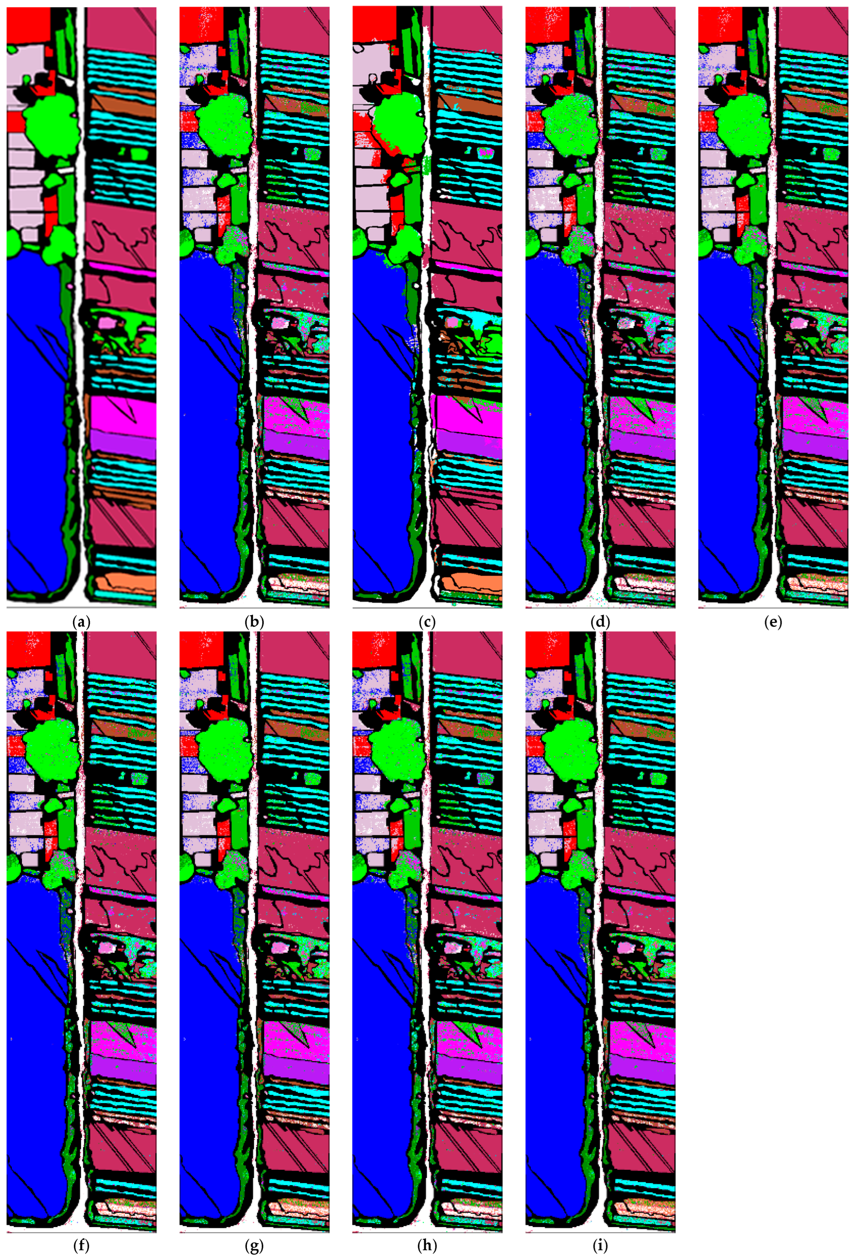
The classification result maps of each model on the WHU-Hi-HanChuan dataset are shown in Figure 11. It can be seen that the classification map of the proposed MSCNN-D-PL (Figure 11i) contains fewer misclassifications.

4.4. Hyperparameter Analysis

In this subsection, four key hyperparameters, i.e., the size of the input sample s, the probability parameter $p$ of Dropout, the number of predictions K for unlabeled samples, and the confidence threshold $p_t$, which impact the performance of the proposed MSCNN-D-PL, are analyzed in detail.

4.4.1. The Size of the Input Sample

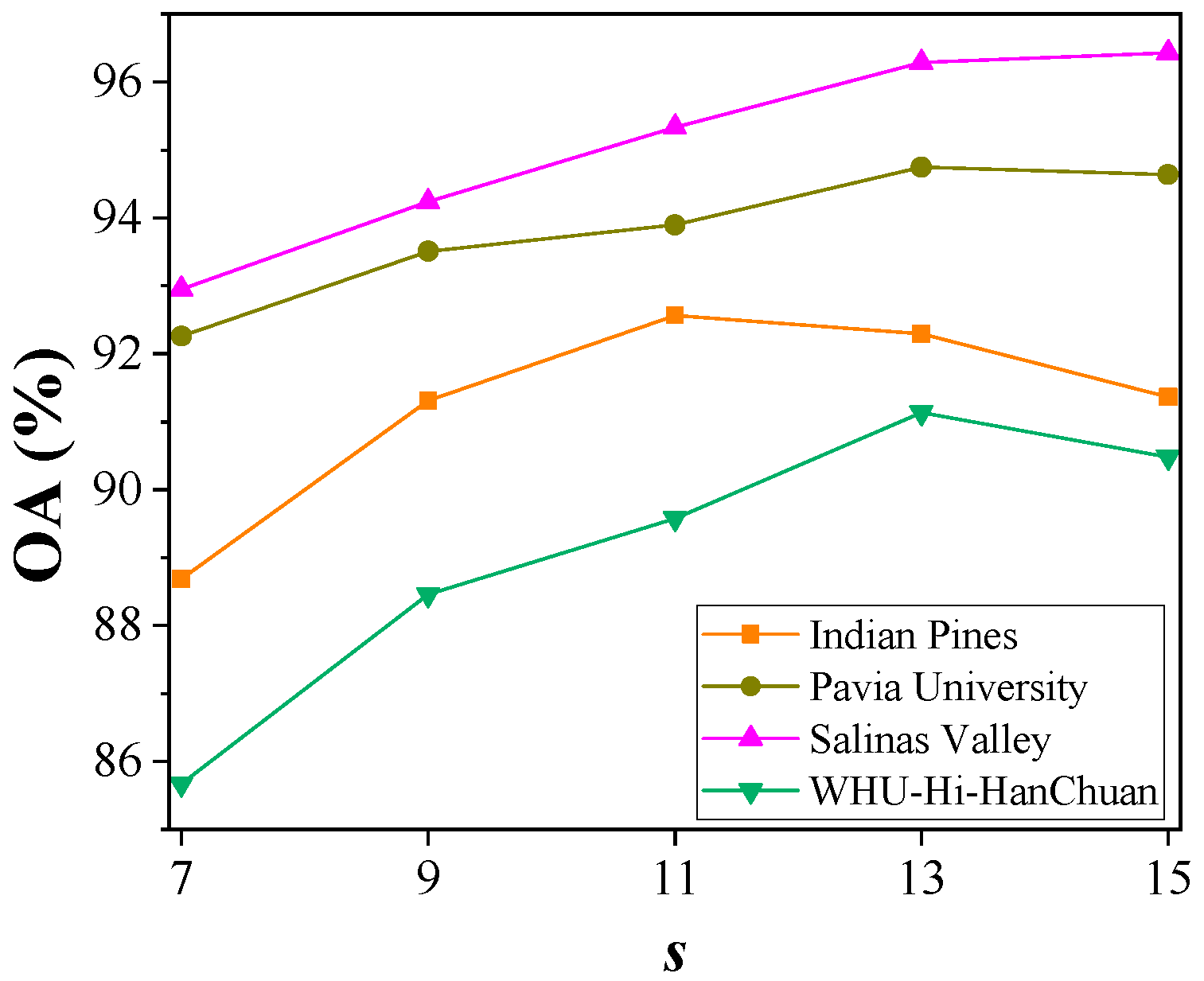
The size of the input sample, i.e., the hyperparameter s, is an important parameter for the proposed MSCNN-D-PL, as it controls the amount of spatial information contained in each input sample and influences the classification performance. In this experiment, the hyperparameter s was set to {7, 9, 11, 13, 15} for all four datasets.

Figure 12 shows the classification accuracy of the proposed MSCNN-D-PL versus the value of the hyperparameter s. It can be seen that for the Indian Pines dataset, the classification accuracy of the MSCNN-D-PL first increases and then decreases as the s value increases. This is because the sample contains less spatial information when s is small, and more spatial information is added as s increases. The classification accuracy (OA) of the model is the highest when s is 11. This is due to the low spatial resolution of the Indian Pines dataset and the complex distribution of ground objects. Therefore, the additional irrelevant information reduces the separability of the samples when s continues to increase (beyond 11), resulting in a decreasing trend in classification accuracy. For the Pavia University dataset, the classification accuracy first increases and then tends to become stable as the s value increases. The classification performance is the best when s is 13. The classification accuracy does not decrease when the hyperparameter s is equal to 15. This may be because the spatial resolution of the Pavia University dataset is 1.3 m, which is higher than that of the Indian Pines dataset at 20 m. Therefore, the purity of the sample can be maintained when s is 15. For the Salinas Valley dataset, the classification accuracy gradually increases with the increase in the hyperparameter s. This may be because the Salinas Valley dataset has high spatial resolution and regular ground object distribution. For the WHU-Hi-HanChuan dataset, given its high spatial resolution, the OA increases rapidly with the hyperparameter s and reaches the maximum value when s equals 13. However, it should be noted that the larger the value of the hyperparameter s, the more data the model needs to process. This results in longer training time and more hardware requirements.

4.4.2. Dropout Probability

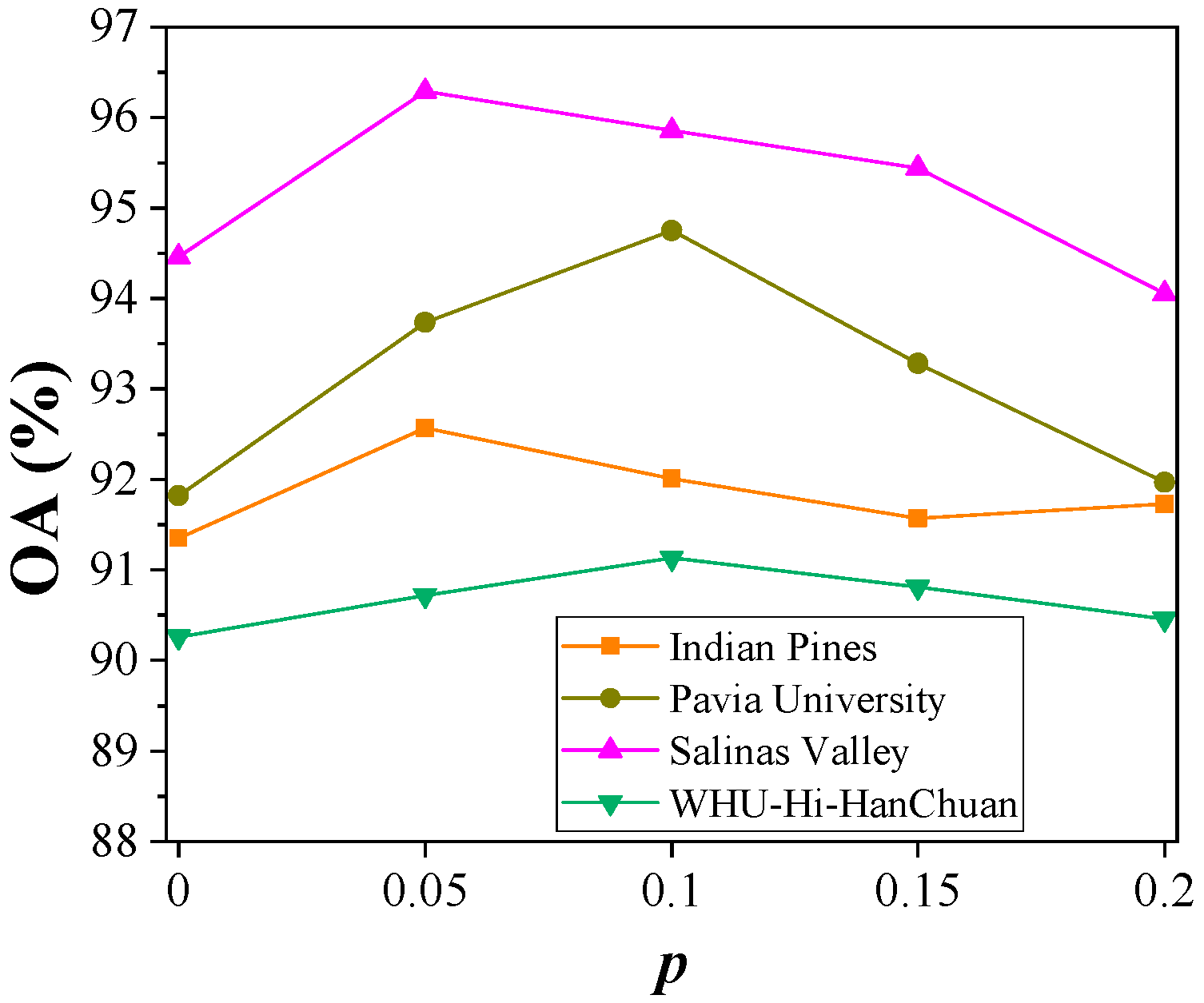
The hyperparameter p, with a range of [0, 1], represents the probability that the Dropout layer randomly discards neural units at the corresponding layer. When the value of p is 0, the Dropout operation is not performed. A large value of p makes the model difficult to train and can even lead to underfitting. In this experiment, we set p to vary between 0 and 0.2, with an interval of 0.05, for all four datasets. The corresponding OAs are presented in Figure 13.

As one can see from the figure, for the Indian Pines dataset, the MSCNN-D-PL achieves the optimal classification accuracy when p is 0.05, whereas the classification performance decreases and tends to become stable with the increase in p. The classification accuracies on the Pavia University and WHU-Hi-HanChuan datasets behave similarly with respect to the hyperparameter p; i.e., as the value of p increases, the OA first increases and then decreases. The highest OA is achieved when the hyperparameter p is 0.1. This indicates that as the hyperparameter p increases, Dropout plays an increasingly important role in improving the performance of the proposed MSCNN-D-PL. However, an excessively large value of p degrades the classification performance. For the Salinas Valley dataset, the MSCNN-D-PL also achieves optimal classification performance when p is set to 0.05. The classification accuracy gradually decreases with increasing p. When p is 0.2, the corresponding classification accuracy is lower than that of the model without Dropout (p = 0). Finally, for the Indian Pines, Pavia University, Salinas Valley, and WHU-Hi-HanChuan datasets, the hyperparameter p was set as 0.05, 0.1, 0.05, and 0.1, respectively, to optimize the performance of the proposed MSCNN-D-PL.

4.4.3. Number of Predictions

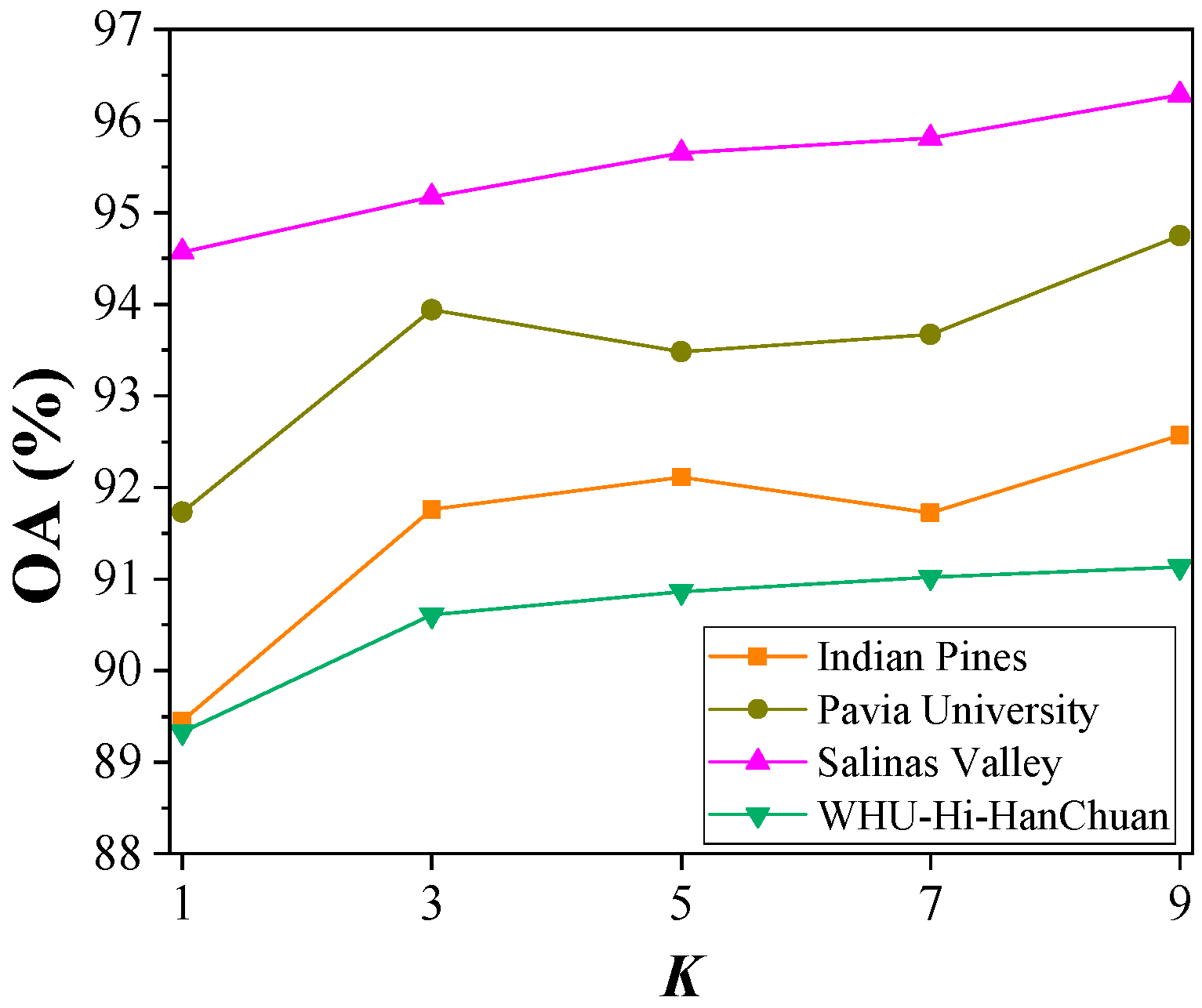
The number of predictions, i.e., the hyperparameter K, controls the number of category probability vectors for each unlabeled sample predicted by the model. Therefore, in general, a larger K will make the final label of the unlabeled sample more accurate, but it will also consume more time in the model training process. In order to fully examine the impact of the hyperparameter K on the performance of the MSCNN-D-PL, in our experiments, the K value was varied in the range of [1, 9] with an interval of 2.

Figure 14 illustrates the influence of the hyperparameter K on the OA of the proposed MSCNN-D-PL. One can see that the classification accuracy of the MSCNN-D-PL on the Indian Pines dataset increases when increasing the K value. The model showed a similar pattern on the Pavia University dataset. The increasing trend is more obvious for the Salinas Valley and WHU-Hi-HanChuan datasets. Therefore, the experimental results on all four datasets show that a larger number of predictions for unlabeled samples leads to higher accuracy of the pseudo-labels, which further improves the classification performance of the MSCNN-D-PL. Therefore, the value of the hyperparameter K is taken as 9 for all four datasets.

4.4.4. Probability Threshold

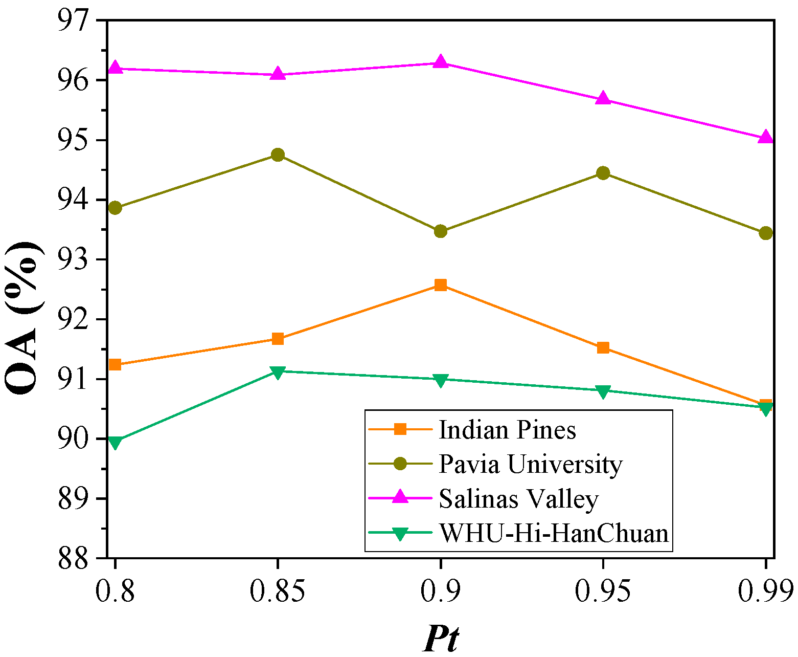
After obtaining the category labels of all unlabeled data, the unlabeled samples with high confidence were selected to expand the training set. The probability threshold, i.e., the hyperparameter $p_t$, controls the confidence level of the selected unlabeled samples. Larger values of $p_t$ indicate higher confidence levels for the selected unlabeled samples, but correspond to smaller numbers of unlabeled samples selected to expand the training set. Therefore, to comprehensively measure the effect of the hyperparameter $p_t$ on the performance of the MSCNN-D-PL, in this experiment, the values of the hyperparameter $p_t$ were set to {0.8, 0.85, 0.9, 0.95, 0.99}. The results obtained on the four datasets are shown in Figure 15.

From the results, one can see that for the Indian Pines and WHU-Hi-HanChuan datasets, the classification accuracy of the proposed MSCNN-D-PL first increases and then decreases as the hyperparameter $p_t$ increases. The model achieves the best accuracy on both datasets when the hyperparameter $p_t$ is set to 0.9 and 0.85, respectively, indicating that these values best balance the quality and quantity of pseudo-labeled samples. For the Pavia University dataset, the performance of the proposed model does not follow a clear trend when increasing the value of $p_t$. The best and second-best classification accuracies are achieved with $p_t$ values of 0.85 and 0.95, respectively. For the Salinas Valley dataset, the classification accuracy tends to decrease as the hyperparameter $p_t$ increases, possibly because the Salinas Valley dataset is relatively easy to classify. Therefore, a low value of the hyperparameter $p_t$ can ensure that many high-quality pseudo-labeled samples are selected to expand the training set. To ensure the best accuracy of the MSCNN-D-PL, the hyperparameter $p_t$ was taken as 0.9, 0.85, 0.8, and 0.85 for the Indian Pines, Pavia University, Salinas Valley, and WHU-Hi-HanChuan datasets, respectively.

4.5. Discussion

In this subsection, the effectiveness and efficiency of the proposed model are further discussed.

4.5.1. Ablation Study

To verify the effectiveness of the proposed method, we conducted ablation experiments on the MSCNN classifier and the Dropout-based pseudo-label generation strategy involved in the proposed MSCNN-D-PL model. The experimental results are reported in

Table 13. Quantitative comparisons among ablation studies on the four considered datasets. MS is multi-scale, and D-PL is the Dropout-based pseudo-label generation strategy.

Method	Indian Pines		Pavia University		Salinas Valley		WHU-Hi-HanChuan
	OA (%)	Kappa (%)	OA (%)	Kappa (%)	OA (%)	Kappa (%)	OA (%)	Kappa (%)
FDSSC (baseline)	86.07 ± 2.41	84.04 ± 2.48	87.21 ± 1.71	82.62 ± 2.08	89.03 ± 1.68	87.77 ± 1.69	84.61 ± 1.83	81.85 ± 2.23
baseline + MS (MSCNN)	89.26 ± 1.21	87.77 ± 1.26	89.81 ± 1.47	85.91 ± 1.89	91.41 ± 1.81	90.37 ± 1.82	86.24 ± 0.98	83.83 ± 1.15
Baseline + MS + D-PL (MSCNN-D-PL)	92.57 ± 0.79	91.52 ± 0.92	94.75 ± 1.93	93.03 ± 2.55	96.29 ± 1.15	95.87 ± 1.28	91.13 ± 0.55	89.58 ± 0.65

. One can see that, on the four datasets, the proposed MSCNN improves the OA from 86.07%, 87.21%, 89.03%, and 84.61% to 89.26%, 89.81%, 91.41%, and 86.24%, respectively, as compared to the baseline. After further integrating the presented Dropout-based pseudo-label generation strategy, i.e., MSCNN-D-PL, the OA is further improved by 3.31%, 4.94%, 4.88%, and 4.89%, respectively, compared to the MSCNN. The results of the ablation experiment show that both our proposed MSCNN classifier and Dropout-based pseudo-label generation strategy contribute to the improved HSI classification accuracy under a limited labeled samples.

4.5.2. Accuracy Versus the Number of Training Samples

To assess the impact of different numbers of training samples on model performance, we compared the classification accuracy of different methods with limited training samples. For the Indian Pines dataset, we randomly selected 1%, 2%, and 5% of training samples from each class, and for the Pavia University, Salinas Valley, and WHU-Hi-HanChuan datasets, we randomly selected 0.1%, 0.2%, and 0.5% of training samples per class, respectively. The experimental results are shown in Figure 16. As one can see, the proposed MSCNN-D-PL achieves the optimal OA in most cases, which demonstrates the excellent generalization ability of our method. Moreover, it is worth emphasizing that the smaller the percentage of training samples, the greater the advantage of our method, which suggests its better capability to address real scenarios with insufficient labeled samples.

4.5.3. Complexity Analysis

To analyze the computational load of the MSCNN-D-PL, we compared the running times of different methods on the four datasets.

Table 14. Results of running time (s) and parameter size (MB) on the four considered datasets. (# Samples is the number of samples)

Dataset	Stage	# Samples	Methods
			MSCNN	DSR-GCN	3D-GAN	PseudoLabel	MeanTeacher	MixMatch	FixMatch	MSCNN-D-PL
Indian Pines	Train	105	215.86	66.65	428.23	232.52	390.26	400.52	405.77	393.38
	Test	10,261	2.38	0.41	1.29	2.40	2.36	2.43	2.33	2.32
	Parameters		2.31	0.33	4.28	2.31	2.31	2.31	2.31	2.31
Pavia University	Train	43	35.96	110.19	106.41	38.03	61.58	64.62	68.49	62.23
	Test	42,733	5.63	0.31	2.64	5.66	5.70	5.61	5.60	5.68
	Parameters		1.20	3.64	2.23	1.20	1.20	1.20	1.20	1.20
Salinas Valley	Train	54	123.33	193.63	243.89	129.52	185.59	189.43	191.30	184.95
	Test	54,075	13.20	0.19	6.91	13.18	13.11	13.21	13.23	13.14
	Parameters		2.36	0.38	4.37	2.36	2.36	2.36	2.36	2.36
WHU-Hi-HanChuan	Train	258	1799.04	722.78	2975.71	1851.84	2306.44	2311.96	2348.55	2257.07
	Test	257,272	91.72	0.80	44.83	92.03	91.85	92.38	91.67	91.53
	Parameters		3.16	0.29	5.85	3.16	3.16	3.16	3.16	3.16

reports the training and testing times of the methods in detail. One can observe that DSR-GCN requires the least testing time on all datasets, which is likely because the graph convolutional network in DSR-GCN tends to have a very fast inference speed after converting the HSI data into graph-structured data. The 3D-GAN model has the longest training time due to its adversarial training strategy, which makes training difficult, yet it requires relatively little testing time due to the simple network it employs. PseudoLabel, MeanTeacher, MixMatch, FixMatch, and MSCNN-D-PL have similar testing times to the MSCNN, as all of them use the MSCNN as the basic classifier. In terms of training time, PseudoLabel, MeanTeacher, MixMatch, FixMatch, and MSCNN-D-PL consume more time than the MSCNN because they need to execute additional semi-supervised strategies. It can also be seen that PseudoLabel, with a simpler pseudo-label generation strategy, requires less training time. Considering the classification performance and running time comprehensively, we can conclude that the proposed MSCNN-D-PL is able to achieve the best classification performance with the same test time as the semi-supervised models using the same basic classifier (MSCNN). Nonetheless, there is still room to reduce the running time of the MSCNN-D-PL compared to DSR-GCN. Therefore, designing a lightweight model to speed up the inference will be our future goal. Regarding the number of trainable parameters in the models, since the comparison methods PseudoLabel, MeanTeacher, MixMatch, and FixMatch, and the proposed MSCNN-D-PL method all employ the MSCNN as the benchmark classifier, these models share the same number of trainable parameters, which is positively correlated with the number of bands in the dataset. The 3D-GAN model, in addition to the classifier, also includes a generator, thus possessing a larger number of trainable parameters. DSR-GCN, a graph convolutional neural network-based model, exhibits the fewest parameters across the Indian Pines, Salinas Valley, and WHU-Hi-HanChuan datasets, yet it has the highest parameter count on the Pavia University dataset. This indicates that the number of parameters in DSR-GCN is primarily influenced by the hyperparameters configured in the model.

5. Conclusions

In this paper, we propose a semi-supervised HSI classification approach based on the combination of a multi-scale convolutional neural network with a Dropout-based pseudo-label strategy. First, a multi-scale convolutional neural network, i.e., MSCNN, was constructed, with the aim of obtaining high-reliability predictions for unlabeled data. Then, a new Dropout-based pseudo-label generation strategy was designed to reduce errors in label generation. Finally, the MSCNN-D-PL was designed by combining the proposed MSCNN model and the pseudo-label strategy to improve HSI classification performance in practical applications with small amounts of labeled data. In the experimental phase, we first verified the effectiveness of the designed MSCNN. Then, we confirmed that typical data augmentation strategies are not suitable for the HSI classification task. Experimental results on four HSI datasets demonstrate that the proposed MSCNN-D-PL achieves the best classification performance compared to state-of-the-art semi-supervised methods.

In future work, we will continue to explore effective and lightweight classification models that can better capture the characteristics of HSI data while reducing running time, as well as design more robust pseudo-label strategies to improve the HSI classification performance with an extremely low number of labeled samples.

References

1. Bioucas-Dias, J.M.; Plaza, A.; Camps-Valls, G.; Scheunders, P.; Nasrabadi, N.; Chanussot, J. Hyperspectral Remote Sensing Data Analysis and Future Challenges. IEEE Geosci. Remote Sens. Mag. 2013, 1, 6–36. [Google Scholar] [CrossRef]
2. Ghamisi, P.; Yokoya, N.; Li, J.; Liao, W.; Liu, S.; Plaza, J.; Rasti, B.; Plaza, A. Advances in Hyperspectral Image and Signal Processing: A Comprehensive Overview of the State of the Art. IEEE Geosci. Remote Sens. Mag. 2017, 5, 37–78. [Google Scholar] [CrossRef]
3. Ribeiro, R.; Cruz, G.; Matos, J.; Bernardino, A. A Data Set for Airborne Maritime Surveillance Environments. IEEE Trans. Circuits Syst. Video Technol. 2019, 29, 2720–2732. [Google Scholar] [CrossRef]
4. Yokoya, N.; Chan, J.; Segl, K. Potential of Resolution-Enhanced Hyperspectral Data for Mineral Mapping Using Simulated EnMAP and Sentinel-2 Images. Remote Sens. 2016, 8, 172. [Google Scholar] [CrossRef]
5. McCann, C.; Repasky, K.S.; Lawrence, R.; Powell, S. Multi-Temporal Mesoscale Hyperspectral Data of Mixed Agricultural and Grassland Regions for Anomaly Detection. ISPRS J. Photogramm. Remote Sens. 2017, 131, 121–133. [Google Scholar] [CrossRef]
6. Huang, X.; Zhang, L. An Adaptive Mean-Shift Analysis Approach for Object Extraction and Classification from Urban Hyperspectral Imagery. IEEE Trans. Geosci. Remote Sens. 2008, 46, 4173–4185. [Google Scholar] [CrossRef]
7. Duan, P.; Hu, S.; Kang, X.; Li, S. Shadow Removal of Hyperspectral Remote Sensing Images with Multiexposure Fusion. IEEE Trans. Geosci. Remote Sens. 2022, 60, 5537211. [Google Scholar] [CrossRef]
8. Duan, P.; Ghamisi, P.; Kang, X.; Rasti, B.; Li, S.; Gloaguen, R. Fusion of Dual Spatial Information for Hyperspectral Image Classification. IEEE Trans. Geosci. Remote Sens. 2021, 59, 7726–7738. [Google Scholar] [CrossRef]
9. Paoletti, M.E.; Haut, J.M.; Plaza, J.; Plaza, A. Deep Learning Classifiers for Hyperspectral Imaging: A Review. ISPRS J. Photogramm. Remote Sens. 2019, 158, 279–317. [Google Scholar] [CrossRef]
10. Chen, Y.; Lin, Z.; Zhao, X.; Wang, G.; Gu, Y. Deep Learning-Based Classification of Hyperspectral Data. IEEE J. Sel. Top. Appl. Earth Obs. Remote Sens. 2014, 7, 2094–2107. [Google Scholar] [CrossRef]
11. Ma, X.; Wang, H.; Geng, J. Spectral–Spatial Classification of Hyperspectral Image Based on Deep Auto-Encoder. IEEE J. Sel. Top. Appl. Earth Obs. Remote Sens. 2016, 9, 4073–4085. [Google Scholar]
12. Chen, Y.; Zhao, X.; Jia, X. Spectral–Spatial Classification of Hyperspectral Data Based on Deep Belief Network. IEEE J. Sel. Top. Appl. Earth Obs. Remote Sens. 2015, 8, 2381–2392. [Google Scholar] [CrossRef]
13. Zhong, P.; Gong, Z.; Li, S.; Schonlieb, C.-B. Learning to Diversify Deep Belief Networks for Hyperspectral Image Classification. IEEE Trans. Geosci. Remote Sens. 2017, 55, 3516–3530. [Google Scholar] [CrossRef]
14. Yue, J.; Zhao, W.; Mao, S.; Liu, H. Spectral–Spatial Classification of Hyperspectral Images Using Deep Convolutional Neural Networks. Remote Sens. Lett. 2015, 6, 468–477. [Google Scholar] [CrossRef]
15. Chen, Y.; Jiang, H.; Li, C.; Jia, X.; Ghamisi, P. Deep Feature Extraction and Classification of Hyperspectral Images Based on Convolutional Neural Networks. IEEE Trans. Geosci. Remote Sens. 2016, 54, 6232–6251. [Google Scholar] [CrossRef]
16. Cheng, G.; Li, Z.; Han, J.; Yao, X.; Guo, L. Exploring Hierarchical Convolutional Features for Hyperspectral Image Classification. IEEE Trans. Geosci. Remote Sens. 2018, 56, 6712–6722. [Google Scholar] [CrossRef]
17. Ben Hamida, A.; Benoit, A.; Lambert, P.; Ben Amar, C. 3-D Deep Learning Approach for Remote Sensing Image Classification. IEEE Trans. Geosci. Remote Sens. 2018, 56, 4420–4434. [Google Scholar] [CrossRef]
18. Paoletti, M.E.; Haut, J.M.; Fernandez-Beltran, R.; Plaza, J.; Plaza, A.J.; Pla, F. Deep Pyramidal Residual Networks for Spectral–Spatial Hyperspectral Image Classification. IEEE Trans. Geosci. Remote Sens. 2019, 57, 740–754. [Google Scholar] [CrossRef]
19. He, N.; Paoletti, M.E.; Haut, J.M.; Fang, L.; Li, S.; Plaza, A.; Plaza, J. Feature Extraction with Multiscale Covariance Maps for Hyperspectral Image Classification. IEEE Trans. Geosci. Remote Sens. 2019, 57, 755–769. [Google Scholar] [CrossRef]
20. Mou, L.; Ghamisi, P.; Zhu, X.X. Deep Recurrent Neural Networks for Hyperspectral Image Classification. IEEE Trans. Geosci. Remote Sens. 2017, 55, 3639–3655. [Google Scholar] [CrossRef]
21. Hang, R.; Liu, Q.; Hong, D.; Ghamisi, P. Cascaded Recurrent Neural Networks for Hyperspectral Image Classification. IEEE Trans. Geosci. Remote Sens. 2019, 57, 5384–5394. [Google Scholar]
22. Ranjan, P.; Girdhar, A. A Comparison of Deep Learning Algorithms Dealing with Limited Samples in Hyperspectral Image Classification. In Proceedings of the 2022 OPJU International Technology Conference on Emerging Technologies for Sustainable Development (OTCON), Raigarh, Chhattisgarh, India, 8–10 February 2023; pp. 1–6. [Google Scholar]
23. Huang, L.; Chen, Y. Dual-Path Siamese CNN for Hyperspectral Image Classification with Limited Training Samples. IEEE Geosci. Remote Sens. Lett. 2021, 18, 518–522. [Google Scholar] [CrossRef]
24. Zhou, L.; Zhu, J.; Yang, J.; Geng, J. Data Augmentation and Spatial-Spectral Residual Framework for Hyperspectral Image Classification Using Limited Samples. In Proceedings of the 2022 IEEE International Conference on Unmanned Systems (ICUS), Guangzhou, China, 28–30 October 2022; pp. 1–6. [Google Scholar]
25. Xue, Z.; Zhang, M.; Liu, Y.; Du, P. Attention-Based Second-Order Pooling Network for Hyperspectral Image Classification. IEEE Trans. Geosci. Remote Sens. 2021, 59, 9600–9615. [Google Scholar]
26. Duan, P.; Xie, Z.; Kang, X.; Li, S. Self-Supervised Learning-Based Oil Spill Detection of Hyperspectral Images. Sci. China Technol. Sci. 2022, 65, 793–801. [Google Scholar]
27. Xue, Z.; Zhou, Y.; Du, P. S3Net: Spectral–Spatial Siamese Network for Few-Shot Hyperspectral Image Classification. IEEE Trans. Geosci. Remote Sens. 2022, 60, 5531219. [Google Scholar] [CrossRef]
28. Yang, X.; Song, Z.; King, I.; Xu, Z. A Survey on Deep Semi-Supervised Learning. IEEE Trans. Knowl. Data Eng. 2023, 35, 8934–8954. [Google Scholar] [CrossRef]
29. Goodfellow, I.J.; Pouget-Abadie, J.; Mirza, M.; Xu, B.; Warde-Farley, D.; Ozair, S.; Courville, A.; Bengio, Y. Generative Adversarial Nets. In Proceedings of the Advances in Neural Information Processing Systems, Montreal, QC, Canada, 8–13 December 2014; Curran Associates, Inc.: Red Hook, NY, USA, 2014; Volume 27. [Google Scholar]
30. Zhan, Y.; Hu, D.; Wang, Y.; Yu, X. Semisupervised Hyperspectral Image Classification Based on Generative Adversarial Networks. IEEE Geosci. Remote Sens. Lett. 2018, 15, 212–216. [Google Scholar] [CrossRef]
31. Zhong, Z.; Li, J.; Clausi, D.A.; Wong, A. Generative Adversarial Networks and Conditional Random Fields for Hyperspectral Image Classification. IEEE Trans. Cybern. 2020, 50, 3318–3329. [Google Scholar]
32. Büchel, J.; Ersoy, O. Ladder Networks for Semi-Supervised Hyperspectral Image Classification. arXiv 2018, arXiv:1812.01222. [Google Scholar] [CrossRef]
33. Rasmus, A.; Valpola, H.; Honkala, M.; Berglund, M.; Raiko, T. Semi-Supervised Learning with Ladder Networks. In Proceedings of the 29th International Conference on Neural Information Processing Systems, Montreal, Canada, 7–12 December 2015; pp. 3546–3554. [Google Scholar]
34. Qin, A.; Shang, Z.; Tian, J.; Wang, Y.; Zhang, T.; Tang, Y.Y. Spectral–Spatial Graph Convolutional Networks for Semisupervised Hyperspectral Image Classification. IEEE Geosci. Remote Sens. Lett. 2019, 16, 241–245. [Google Scholar] [CrossRef]
35. Sha, A.; Wang, B.; Wu, X.; Zhang, L. Semisupervised Classification for Hyperspectral Images Using Graph Attention Networks. IEEE Geosci. Remote Sens. Lett. 2021, 18, 157–161. [Google Scholar] [CrossRef]
36. Xie, Y.; Liang, Y.; Gong, M.; Qin, A.K.; Ong, Y.-S.; He, T. Semisupervised Graph Neural Networks for Graph Classification. IEEE Trans. Cybern. 2023, 53, 6222–6235. [Google Scholar] [CrossRef] [PubMed]
37. Wu, H.; Prasad, S. Semi-Supervised Deep Learning Using Pseudo Labels for Hyperspectral Image Classification. IEEE Trans. Image Process. 2018, 27, 1259–1270. [Google Scholar] [CrossRef]
38. Fang, B.; Li, Y.; Zhang, H.; Chan, J. Semi-Supervised Deep Learning Classification for Hyperspectral Image Based on Dual-Strategy Sample Selection. Remote Sens. 2018, 10, 574. [Google Scholar] [CrossRef]
39. Kang, X.; Zhuo, B.; Duan, P. Semi-Supervised Deep Learning for Hyperspectral Image Classification. Remote Sens. Lett. 2019, 10, 353–362. [Google Scholar] [CrossRef]
40. Berthelot, D.; Carlini, N.; Goodfellow, I.; Papernot, N.; Oliver, A.; Raffel, C. MixMatch: A Holistic Approach to Semi-Supervised Learning. In Proceedings of the 33rd International Conference on Neural Information Processing Systems, Vancouver, BC, Canada, 8–14 December 2019; pp. 5049–5059. [Google Scholar]
41. Sohn, K.; Berthelot, D.; Li, C.-L.; Zhang, Z.; Carlini, N.; Cubuk, E.D.; Kurakin, A.; Zhang, H.; Raffel, C. FixMatch: Simplifying Semi-Supervised Learning with Consistency and Confidence. In Proceedings of the 34th International Conference on Neural Information Processing Systems, Vancouver, BC, Canada, 6–12 December 2020; pp. 596–608. [Google Scholar]
42. Srivastava, N.; Hinton, G.; Krizhevsky, A.; Sutskever, I.; Salakhutdinov, R. Dropout: A Simple Way to Prevent Neural Networks from Overfitting. J. Mach. Learn. Res. 2014, 15, 1929–1958. [Google Scholar]
43. Zhang, H.; Li, Y.; Zhang, Y.; Shen, Q. Spectral-Spatial Classification of Hyperspectral Imagery Using a Dual-Channel Convolutional Neural Network. Remote Sens. Lett. 2017, 8, 438–447. [Google Scholar] [CrossRef]
44. Yang, J.; Zhao, Y.; Chan, J.C.-W.; Yi, C. Hyperspectral Image Classification Using Two-Channel Deep Convolutional Neural Network. In Proceedings of the 2016 IEEE International Geoscience and Remote Sensing Symposium (IGARSS), Beijing, China, 10–15 July 2016; pp. 5079–5082. [Google Scholar]
45. Hao, S.; Wang, W.; Ye, Y.; Nie, T.; Bruzzone, L. Two-Stream Deep Architecture for Hyperspectral Image Classification. IEEE Trans. Geosci. Remote Sens. 2018, 56, 2349–2361. [Google Scholar]
46. Li, Y.; Zhang, H.; Shen, Q. Spectral–Spatial Classification of Hyperspectral Imagery with 3D Convolutional Neural Network. Remote Sens. 2017, 9, 67. [Google Scholar] [CrossRef]
47. Paoletti, M.E.; Haut, J.M.; Plaza, J.; Plaza, A. A New Deep Convolutional Neural Network for Fast Hyperspectral Image Classification. ISPRS J. Photogramm. Remote Sens. 2018, 145, 120–147. [Google Scholar] [CrossRef]
48. Zhong, Z.; Li, J.; Luo, Z.; Chapman, M. Spectral–Spatial Residual Network for Hyperspectral Image Classification: A 3-D Deep Learning Framework. IEEE Trans. Geosci. Remote Sens. 2018, 56, 847–858. [Google Scholar] [CrossRef]
49. Wang, W.; Dou, S.; Jiang, Z.; Sun, L. A Fast Dense Spectral–Spatial Convolution Network Framework for Hyperspectral Images Classification. Remote Sens. 2018, 10, 1068. [Google Scholar]
50. He, K.; Zhang, X.; Ren, S.; Sun, J. Deep Residual Learning for Image Recognition. In Proceedings of the 2016 IEEE Conference on Computer Vision and Pattern Recognition (CVPR), Las Vegas, NV, USA, 27–30 June 2016; pp. 770–778. [Google Scholar]
51. Huang, G.; Liu, Z.; Van Der Maaten, L.; Weinberger, K.Q. Densely Connected Convolutional Networks. In Proceedings of the 2017 IEEE Conference on Computer Vision and Pattern Recognition (CVPR), Honolulu, HI, USA, 21–26 July 2017; pp. 2261–2269. [Google Scholar]
52. Szegedy, C.; Liu, W.; Jia, Y.; Sermanet, P.; Reed, S.; Anguelov, D.; Erhan, D.; Vanhoucke, V.; Rabinovich, A. Going Deeper with Convolutions. In Proceedings of the 2015 IEEE Conference on Computer Vision and Pattern Recognition (CVPR), Boston, MA, USA, 7–12 June 2015; pp. 1–9. [Google Scholar]
53. Ioffe, S.; Szegedy, C. Batch Normalization: Accelerating Deep Network Training by Reducing Internal Covariate Shift. arXiv 2015, arXiv:1502.03167. [Google Scholar] [CrossRef]
54. Vinod, N.; Geoffrey, E.H. Rectified linear units improve restricted boltzmann machines. In Proceedings of the 27th International Conference on International Conference on Machine Learning, Haifa, Israel, 21–24 June 2010; pp. 807–814. [Google Scholar]
55. Bouthillier, X.; Konda, K.; Vincent, P.; Memisevic, R. Dropout as data augmentation. arXiv 2015, arXiv:1506.08700. [Google Scholar] [CrossRef]
56. Zhao, D.; Yu, G.; Xu, P.; Luo, M. Equivalence between Dropout and Data Augmentation: A Mathematical Check. Neural Netw. 2019, 115, 82–89. [Google Scholar] [CrossRef] [PubMed]
57. Available online: https://pytorch.org/ (accessed on 25 March 2023).
58. Zhong, Y.; Hu, X.; Luo, C.; Wang, X.; Zhao, J.; Zhang, L. WHU-Hi: UAV-Borne Hyperspectral with High Spatial Resolution (H2) Benchmark Datasets and Classifier for Precise Crop Identification Based on Deep Convolutional Neural Network with CRF. Remote Sens. Environ. 2020, 250, 112012. [Google Scholar] [CrossRef]
59. Zhong, Y.; Wang, X.; Xu, Y.; Wang, S.; Jia, T.; Hu, X.; Zhao, J.; Wei, L.; Zhang, L. Mini-UAV-Borne Hyperspectral Remote Sensing: From Observation and Processing to Applications. IEEE Geosci. Remote Sens. Mag. 2018, 6, 46–62. [Google Scholar] [CrossRef]
60. Xue, Z.; Liu, Z.; Zhang, M. DSR-GCN: Differentiated-Scale Restricted Graph Convolutional Network for Few-Shot Hyperspectral Image Classification. IEEE Trans. Geosci. Remote Sens. 2023, 61, 5504918. [Google Scholar] [CrossRef]
61. Tarvainen, A.; Valpola, H. Mean teachers are better role models: Weight-averaged consistency targets improve semi-supervised deep learning results. In Proceedings of the 31st International Conference on Neural Information Processing Systems, Long Beach, CA, USA, 4–9 December 2017; pp. 1195–1204. [Google Scholar]
62. Kingma, D.P.; Ba, J. Adam: A Method for Stochastic Optimization. In Proceedings of the 3rd International Conference on Learning Representations, San Diego, CA, USA, 7–9 May 2015. [Google Scholar]
63. Xue, Z.; Xu, Q.; Zhang, M. Local Transformer with Spatial Partition Restore for Hyperspectral Image Classification. IEEE J. Sel. Top. Appl. Earth Obs. Remote Sens. 2022, 15, 4307–4325. [Google Scholar] [CrossRef]
64. Cubuk, E.D.; Zoph, B.; Shlens, J.; Le, Q.V. RandAugment: Practical Automated Data Augmentation with a Reduced Search Space. In Proceedings of the Conference on Computer Vision and Pattern Recognition Workshops (CVPRW), Seattle, WA, USA, 14–19 June 2020. [Google Scholar]
Figure 1. Structure of the FDSSC [49].
Remotesensing 17 03273 g001
Figure 2. Structures of the proposed spectral and spatial multi-scale convolutional blocks. (a) spectral multi-scale convolutional block (SpecMCB); (b) spatial multi-scale convolutional block (SpatMCB).
Remotesensing 17 03273 g002
Figure 3. Structure of the proposed MSCNN.
Remotesensing 17 03273 g003
Figure 4. (a) False-color composite of images of bands 57, 27, and 17; (b) available ground-truth map (Indian Pines dataset).
Remotesensing 17 03273 g004
Figure 5. (a) False-color composite images of bands 102, 56, and 31; (b) available ground-truth map (Pavia University dataset).
Remotesensing 17 03273 g005
Figure 6. (a) False-color composite images of bands 50, 27, and 17; (b) available ground-truth map (Salinas Valley dataset).
Remotesensing 17 03273 g006
Figure 7. (a) False-color composite images of bands 51, 71, and 91; (b) available ground-truth map (WHU-Hi-HanChuan dataset).
Remotesensing 17 03273 g007
Figure 8. Classification maps of different methods on the Indian Pines dataset: (a) ground truth; (b) MSCNN; (c) DSR-GCN; (d) 3D-GAN; (e) PseudoLabel; (f) MeanTeacher; (g) MixMatch; (h) FixMatch; (i) MSCNN-D-PL.
Remotesensing 17 03273 g008
Figure 9. Classification maps of different methods on the Pavia University dataset: (a) ground truth; (b) MSCNN; (c) DSR-GCN; (d) 3D-GAN; (e) PseudoLabel; (f) MeanTeacher; (g) MixMatch; (h) FixMatch; (i) MSCNN-D-PL.
Remotesensing 17 03273 g009
Figure 10. Classification maps of different methods on the Salinas Valley dataset: (a) ground truth; (b) MSCNN; (c) DSR-GCN; (d) 3D-GAN; (e) PseudoLabel; (f) MeanTeacher; (g) MixMatch; (h) FixMatch; (i) MSCNN-D-PL.
Remotesensing 17 03273 g010
Figure 11. Classification maps of different methods on the WHU-Hi-HanChuan dataset: (a) ground truth; (b) MSCNN; (c) DSR-GCN; (d) 3D-GAN; (e) PseudoLabel; (f) MeanTeacher; (g) MixMatch; (h) FixMatch; (i) MSCNN-D-PL.
Remotesensing 17 03273 g011
Figure 12. OA versus the size of input samples s.
Remotesensing 17 03273 g012
Figure 13. OA versus the Dropout probability p.
Remotesensing 17 03273 g013
Figure 14. OA versus the number of predictions K.
Remotesensing 17 03273 g014
Figure 15. OA versus the probability threshold p t .
Remotesensing 17 03273 g015
Figure 16. OA versus the percentage of selected training samples on the four considered datasets: (a) Indian Pines; (b) Pavia University; (c) Salinas Valley; (d) WHU-Hi-HanChuan.
Remotesensing 17 03273 g016