Article

Future Scenarios of Global Urban Expansion and Carbon Emissions with National Heterogeneity: A Mixed-Effects Model Based on Urban Nighttime Lights

Division of Sustainable Energy and Environmental Engineering, Graduate School of Engineering, The University of Osaka, Suita 565-0871, Japan
*
Author to whom correspondence should be addressed.
Remote Sens. 2025, 17(18), 3251; https://doi.org/10.3390/rs17183251
Submission received: 22 August 2025 / Revised: 14 September 2025 / Accepted: 17 September 2025 / Published: 20 September 2025

Abstract

Highlights

What are the main findings?
  • Scenario-based projections of urban expansion and CO2 emissions for 555 global cities from 2017 to 2053 are generated using a mixed-effects model under five Shared Socioeconomic Pathways–Representative Concentration Pathways (SSP–RCP) scenarios.
  • National and regional heterogeneity is evident: developed cities may experience stabilization or even shrinkage under certain scenarios, whereas developing cities, particularly in Asia and Africa, are projected to undergo rapid expansion.
What is the implication of the main finding?
  • Total urban area is projected to increase across all scenarios. In regionally fragmented and socially unequal pathways (e.g., SSP3–RCP6.0), urban growth is constrained but emissions remain high. Meanwhile, high-growth, fossil fuel–driven pathways are associated with extensive urban sprawl and elevated emissions, while sustainable scenarios foster compact, low-carbon development.
  • The results indicate that region-specific policies and early planning are essential to align urbanization trajectories with global climate mitigation goals.

Abstract

Cities play a pivotal role in environmental transformation and climate change mitigation. Urban expansion has substantial impacts on socioeconomic development and carbon emissions. This study develops a predictive model for future urban expansion and CO2 emissions based on nighttime light (NTL) data, under five SSP-RCP scenarios (SSP1–2.6, SSP2–4.5, SSP3–6.0, SSP4–6.0, and SSP5–8.5) projected to 2053. This study introduces three key improvements from previous literature: (1) a mixed-effects model to capture cross- national and regional differences in urban expansion patterns; (2) incorporation of grid-level random effects to reflect inter-city growth heterogeneity; and (3) integration of SSP-RCP scenarios to incorporate the influence of emission efficiency and socioeconomic policies. Using this improved framework, we estimate future urban expansion and carbon emissions for 555 global cities. The results show that the sensitivity of urban expansion to GDP and population growth varies across countries, leading to diverse urban expansion trajectories. Nonetheless, urban areas are projected to increase under all scenarios. Meanwhile, improvements in emission efficiency under the SSP-RCP scenarios are expected to curb future emission trajectories. This study enhances urban scenario modeling and contributes to a better understanding of regional differences in global urban growth and CO2 emissions.

1. Introduction

Urban areas play a pivotal role in global climate change. The World Cities Report 2024 highlights that cities are both key drivers of environmental change and central actors in climate mitigation strategies [1]. Urbanization contributes to land-use change, deforestation, ecosystem fragmentation, biodiversity loss, and local climate variability [2,3,4,5,6], posing major challenges to sustainability. High population density further impacts energy use and GHG emissions, underscoring the importance of studying urban spatial patterns and their evolution in the context of environmental monitoring and sustainable development [7,8].
Existing studies have applied various models—ranging from statistical to AI-based approaches—to predict future urban expansion [9], yet results often diverge. Many rely on land-use or statistical data, which limits spatial precision and the integration of scenario-based forecasting.
Nighttime light (NTL) data, with their high spatial resolution, temporal continuity, and global availability, have become a key tool in urban research [10]. NTL has been widely used to map urban extent [11,12], estimate economic activity [13,14], monitor nighttime behaviors [15], and assess emissions [16]. Recent studies also employ NTL to forecast future urban growth. For example, Kii et al. [17] established a global model linking NTL and socioeconomic indicators, projecting urban expansion and CO2 emissions for over 550 cities under Shared Socioeconomic Pathway (SSP) scenarios.
This study builds on prior work by introducing a Linear Mixed-effects Model (LMM) [18] to better capture interregional and intercity differences in urban growth. The model incorporates national-level and grid-level random effects to reflect socioeconomic and spatial heterogeneity. Additionally, the integration of SSP with Representative Concentration Pathway (RCP) scenarios enhances the understanding of future CO2 estimates [19].
The paper is structured as follows: Section 2 reviews related work and outlines this study’s contributions. Section 3 describes the data, modeling framework, and CO2 emission estimation method. Section 4 presents scenario-based projections of NTL and their applications for urban activities. Section 5 discusses the findings and future directions.

2. Literature Review

2.1. Urban Expansion Studies

Current urban expansion models generally fall into two broad categories: The first focuses on the “why” of expansion, emphasizing causal inference and interpretability by modeling the effects of socioeconomic, geographic, and policy drivers. The second emphasizes the “how,” relying on historical expansion patterns and data-driven techniques to capture spatiotemporal evolution.
The first approach often employs multiple linear regression (MLR) [20], geographically weighted regression (GWR) [21], support vector machine (SVR) [22], and machine learning algorithms such as random forests, artificial neural networks (ANN) [23], and multilayer perceptrons (MLP) [24]. These methods offer strong interpretability and allow quantification of factor contributions to expansion. However, they depend heavily on variable selection and model assumptions, which may limit their ability to represent complex spatial dynamics and heterogeneity.
The second category extracts expansion trajectories from remote sensing or built-up area data and forecasts trends using models like Markov chains [25], cellular automata (CA), the SLEUTH model [26], and deep learning–based image recognition [27]. These approaches leverage large-scale spatiotemporal data, enabling efficient simulations of urban form dynamics, but they often lack integration of non-spatial drivers such as policy or socioeconomic context.
Recent studies increasingly integrate these two approaches to enhance predictive accuracy and realism. Chettry et al. [28] combined ANN-MLP and CA to forecast urban land changes in India; Liu et al. [29] coupled system dynamics (SD) and CA to simulate China’s land use through 2100; Gao et al. [30] used a “CLUBS + SELECT” framework, integrating macro-level driver selection and micro-level evolution under five SSP scenarios to project global urban growth; Chen et al. [31] applied panel regressions and the FLUS model to estimate future urban land demand under SSP scenarios; Kii et al. [17] developed a global expansion and carbon emissions prediction framework centered around NTL, linking macro drivers and micro potential using regression models. This trend toward combining interpretability with spatial dynamics directly informs the present study design. The model integrates socioeconomic drivers at both macro (city-level) and micro (grid-level) scales, while also considering local geographic features and spatial evolution patterns. This dual perspective allows us to generate urban expansion predictions that are both scenario-sensitive and spatially detailed.
Data sources in this field are incorporating traditional statistical data to remote sensing imagery. Compared to conventional statistics—limited by low update frequency, coarse spatial resolution, and inconsistency—remote sensing offers high resolution, frequent coverage, and cross-region comparability, ideal for global and multi-temporal studies. Common imagery sources include Landsat multispectral data [32], MODIS time series [33] and Sentinel-2 images [34], used widely for built-up area detection, land cover classification, and vegetation monitoring.
Nighttime lights (NTL) have recently risen to prominence in urban studies [35]. As a proxy for population and economic activity, NTL provides consistent, annual, global coverage and can supplement regions lacking reliable statistics [36]. NTL data has been widely used for identifying urban extents [37,38], extracting city centers [39], monitoring expansion [40,41,42], and projecting future urban growth [10,17]. The growing body of research applying NTL in cross-regional and long-term urban analysis reinforces its value as a global data source. Accordingly, NTL is employed as a core dataset in the predictive framework, enabling consistent comparisons across cities worldwide.
The above evolution in methods directly shapes our modeling strategy: we adopt a framework that unites “why” (macro, driver-based inference) with “how” (micro, spatial evolution). Concretely, we integrate city-level socioeconomic drivers and grid-level spatial potentials, while incorporating local geographic features and historical spatial evolution patterns, so that our urban growth projections are scenario-sensitive and spatially detailed. Within this framework, NTL—as a globally consistent proxy for human activity—serves as the bridge that links macro socioeconomic conditions to micro spatial allocation [10,17,38,39,40,41,42,43]. This NTL-anchored, mixed-scale design is a deliberate inheritance and synthesis of the two research streams above.

2.2. Urban CO2 Emissions Studies

Urbanization is a dominant driver of global CO2 emissions. Moran et al. [44] reported that in 2015, urban areas accounted for 68% of global carbon footprints, with the top 100 emitting cities responsible for 18%. Spatial modeling and forecasting of urban emissions are thus critical for climate policy.
Existing urban CO2 studies integrate statistical, geographic, and remote sensing data. Wang et al. [45] developed a GIS-based regression and micro-spatial simulation framework for city-level emissions estimation. Among these data sources, NTL has emerged as a particularly valuable proxy. Its global availability, long-term continuity, and cross-country comparability make it especially suitable for worldwide urban modeling. Fang et al. [46] estimated emissions and efficiency for 282 Chinese cities using NTL from 2004 to 2018; Wu et al. [10] employed NTL to quantify how expansion drives CO2 emissions across 41 southwestern Chinese cities; and other studies have used fixed-effects models combining NTL with energy data in the Yangtze River Delta [47].
On the methodological side, diverse approaches have been applied to project future emissions, ranging from regression models to neural networks (e.g., FNN, RNN), other machine learning methods (e.g., SVM, decision trees), and hybrid approaches [48]. While artificial intelligence methods offer high predictive capacity, they often lack transparency in explaining socio-economic pathways, which limits their use for policy-oriented scenario analysis. O’Neill et al. [49] developed a PET model incorporating population, energy, and technology to forecast economic and emissions trajectories.
In contrast, scenario-based approaches provide a clearer policy-relevant framework. Early Shared Socioeconomic Pathways (SSPs) focused on socio-demographic and economic trends, whereas the integration with Representative Concentration Pathways (SSP–RCPs) further incorporates energy policy and emission efficiency evolution. This combination offers a more comprehensive and consistent foundation for urban CO2 projections [17]. For example, Kevin et al. employed SSP–RCP data to assess global urban CO2 emissions from 1990 to 2100 [50].

2.3. Contributions of This Study

While existing models provide various theoretical and data-driven approaches to urban expansion and carbon emissions forecasting, they often fall short in addressing key challenges. Specifically, conventional regression methods struggle to capture both socioeconomic heterogeneity across countries and fine-scale variation within cities, while SSP-only scenario-based models frequently overlook the role of technological and policy-driven changes in emission efficiency.
The methodological evolution reviewed above highlights two clear directions: (1) combining causal, driver-based inference with spatially explicit simulation, and (2) leveraging globally consistent datasets such as NTL to link macro socioeconomic drivers with micro spatial allocation. Our study directly builds on these developments and contributes by advancing an integrated framework that unites them.
This study offers three key innovations to address these limitations: (1) We introduce a Linear Mixed-Effects Model (LMM) that captures both cross-national differences and intra-urban spatial variability, improving the model’s capacity to reflect real-world complexity. (2) By centering the model on NTL data, we construct an integrated framework that links city-level socioeconomic conditions to fine-grained spatial expansion potential, facilitating projections even in data-scarce regions. (3) We combine Shared Socioeconomic Pathways (SSPs) and Representative Concentration Pathways (RCPs) with an emission-efficiency correction factor that accounts for technological and policy developments. This design inherits the strengths of scenario-based modeling and enables more realistic and policy-relevant CO2 emission forecasts.
Using this framework, we simulate urban expansion and CO2 emissions at high spatial resolution across 555 global cities with populations exceeding one million, from 2017 to 2053, with 2017 serving as the base year used for model calibration. All subsequent estimates are generated starting from 2017. The results provide new insights and tools to support evidence-based planning for urban sustainability and climate policy.

3. Materials and Methods

3.1. Framework Overview

This study comprises two main components across macro and micro levels, as is shown in Figure 1. The first component is the urban nighttime light (NTL) prediction model, which aims to estimate the spatial distribution of NTL at the grid level for target cities from 2017 to 2053. This model consists of two parts: macro level and micro level. For macro level, a linear mixed-effects model (LMM) grouped by country is constructed to predict the total urban NTL intensity based on per capita GDP and population, controlling overall NTL growth at the city level. Based on the estimation using the LMM, the variation in the impact of factors across countries is presented. For micro level, we downscale the total NTL to grid level based on the following three steps: (1) A spatial allocation method distributes the annual city-level NTL increments to grids; (2) A grid-level LMM, grouped by city, estimates NTL growth potential based on local geographic and socioeconomic variables as well as changes in neighboring grids; (3) A rank-based matching procedure assigns the final NTL values to individual grid cells by aligning the allocated increments with their estimated growth potentials, thereby ensuring that the spatial distribution reflects both the aggregate city-level growth and local development heterogeneity.
The second component is the urban CO2 emission prediction model. Based on the projected NTL results from the first part, this model estimates the spatial distribution of CO2 emissions at the grid level. A regression model is established using 2017 NTL and CO2 data, and future projections are adjusted using SSP–RCP scenario-based emission data, incorporating a correction method for technological improvements in emission efficiency.
Section 3.2 introduces the data sources used; Section 3.3 details the construction and validation of the NTL prediction model; and Section 3.4 explains the CO2 emission model and its correction mechanism.

3.2. Data Sources and Preprocessing

This study developed a multi-level urban CO2 emission prediction model by integrating remote sensing imagery with socio-economic data. The analysis covers 555 global cities with populations exceeding one million, incorporating both city-scale and grid-scale spatial levels. It includes both historical data and future scenario projections. The historical datasets consist of city population, per capita GDP, NTL intensity, CO2 emissions, and various spatial and environmental variables. These historical data sources and processing methods are consistent with those used in a previous study [17]. The future scenario data cover projections from 2017 to 2053 for population, GDP, and CO2 emissions under multiple SSP-RCP combinations [51].
City-level population data were obtained from the “World Urbanization Prospects” (WUP) by the United Nations. Per capita GDP data were derived from the gridded GDP dataset by Kummu et al. (standardized to constant 2015 USD) and supplemented using World Bank’s World Development Indicators (WDI) through linear interpolation to estimate values for the years 2013, 2017, and 2021 [52]. NTL data were sourced from NASA’s NPP-VIIRS Day/Night Band (DNB) annual median composite imagery (Version 2), which has been available annually since 2013 [53]. All NTL imagery was radiometrically corrected, georeferenced, and standardized to a 1-km spatial resolution.
Urban areas were divided into 500-m square grid cells, from which both static and dynamic spatial variables were extracted. Static variables include distance to the city center, distance to major roads and railway stations, elevation, and slope. The dynamic variable is defined as the average NTL value of the eight neighboring cells from the previous year. Supplementary datasets include road and railway networks from OpenStreetMap, water bodies from the ASTER Global Water Bodies Database (https://www.earthdata.nasa.gov/data/catalog/lpdaac-ecs-astwbd-001, accessed on 1 July 2023), temperature and precipitation data from “WorldClim Version 2” (https://www.worldclim.org/data/worldclim21.html, accessed on 1 July 2023), and elevation and slope information derived from MERIT DEM. The World Database on Protected Areas (WDPA) (https://www.protectedplanet.net/en, accessed on 1 July 2023) was also used to control for the effects of land-use regulation.
CO2 emission data were obtained from the ODIAC high-resolution global CO2 emission dataset [54,55]. The raster layer from 2017 was selected and spatially aligned with city boundaries using NTL data to ensure consistency in spatial distribution.
All economic data were standardized to constant 2015 USD. Missing values were imputed using the median values of corresponding countries or regions to ensure temporal completeness and spatial continuity.
To simulate urban development under different future pathways, this study employed national-level scenario data on population, GDP, and CO2 emissions based on combinations of Shared Socioeconomic Pathways (SSPs) and Representative Concentration Pathways (RCPs). The dataset was compiled by Gütschow et al. [51], derived from Integrated Assessment Model (IAM) outputs and downscaled from regional to national levels using the Index Convergence (IE) method. It provides a harmonized annual time series spanning from 2017 to 2100.
Five typical SSP-RCP combinations were selected: (1) RCP3PD–SSP1: A low-emission, sustainability-focused pathway featuring high equity, low population growth, and a shift to clean energy; (2) RCP4.5–SSP2: A “middle of the road” scenario with moderate challenges to mitigation and adaptation, reflecting historical development trends; (3) RCP6.0–SSP3: A scenario of regional rivalry with low international cooperation, high population growth, and slow technological development; (4) RCP6.0–SSP4: A highly unequal world with disparities in access to resources, where elites benefit from clean technologies while others are left behind; (5) RCP8.5–SSP5: A fossil fuel-intensive development pathway characterized by rapid economic growth, high energy demand, and high emissions. These combinations were chosen based on recommendations from climate assessment reports, such as those by the Intergovernmental Panel on Climate Change (IPCC), as they represent a wide spectrum of plausible socio-economic and environmental futures. The dataset made available by the IIASA modeling team (https://zenodo.org/records/3638137, accessed on 1 April 2025).
Since the SSP-RCP scenario data are only available at the national level, city-scale projections were generated using an indirect estimation approach. Using 2017 as the baseline year, annual national growth rates of population and GDP were applied to each city to estimate future values of population and per capita GDP under each scenario. This enabled the translation of national-level projections into city-scale data for modeling purposes.

3.3. Modeling Framework

3.3.1. Urban Nighttime Light (NTL) Prediction Model

This study develops a two-tiered modeling framework to simulate the spatiotemporal evolution of NTL for 555 global megacities from 2017 to 2053 under five SSP–RCP scenarios. The framework consists of a macro-level model for estimating total city-level NTL intensity and a micro-level model for distributing the intensity across spatial grids.
(i)
Macro-Level Model
At the macro level, an LMM is constructed to estimate the total NTL intensity of each city, grouped by ISO country codes. The dependent variable T N T L i t represents the total NTL intensity of city i in year t , modeled as a function of the total population P O P i t and per capita GDP G D P p c i t .
The selection of these two factors is based on both empirical and practical considerations. Previous studies [17] demonstrated a consistent positive correlation between NTL intensity, population, and GDP per capita, confirming their explanatory power for the urban total NTL intensity. In addition, population and GDP are the core variables projected by the SSP–RCP framework, which ensures consistent and comparable long-term data availability across all countries and cities worldwide. These features make them particularly suitable for scenario-based projections of NTL.
The model incorporates both fixed effects β 0 , β 1 , β 2 and country-level random effects on intercept and slopes. The formal model specification is:
ln T N T L i t = β 0 + β 1 ln P O P i t + β 2 ln G D P p c i t + u 0 , c i + u 1 , c i ln P O P i t + u 2 , c i ln G D P p c i t + ε 1 , i t
In this formulation, β 0 , β 1 , β 2 are fixed-effect coefficients capturing the global trend across cities, u k , c i   k = 0 , 1 , 2 represent country-specific random effects where c i denotes city i in country c , and ε , 1 , i , t denotes the residual error. The model is trained using city-level data from 2013, 2017, and 2021, and is applied to predict total NTL values for each city under five SSP–RCP scenarios from 2017 to 2053 at four-year intervals.
(ii)
Micro-Level Model
At the micro level, the increment in total NTL intensity of city i from year   t 1 to year t , denoted as Δ T N T L t = T N T L t T N T L t 1 , is distributed to individual grid cells through a sequential three-step process.
First, a proportional allocation method is applied to distribute the total NTL increase across all grid cells, based on each grid’s share of the previous year’s total NTL. Let p N T L l t denote the NTL value of grid cell l in year t , where g is the total number of grid cells in the city. The initial allocated value is computed as:
p N T L l t = p N T L l t 1 + p N T L l t 1 l = 1 g p N T L l t 1 Δ T N T L t
Once the NTL values for all grids are estimated, they are sorted in descending order to form a reference sequence for rank-based matching. Let p N T L t represent this ordered set, where N T L j t is the j-th largest value:
p N T L t = { p N T L j t j 1 , g }       w h e r e   p N T L j 1 t p N T L j t
Second, the NTL growth potential of each grid cell, representing its future urbanization potential, is estimated using an LMM based on spatial, socioeconomic, and environmental variables. Random effects are grouped by city. The model is specified as:
P m , n t = k 1 K 1 α k 1 + γ k 1 , i x k 1 , m , n t + k 2 K 2 α k 2 x k 2 , m , n t + ε 2 , m , n t
Here, P m , n t is the potential value of grid cell m , n in year t . The set K 1 includes variables with both fixed and random effects, while K 2 includes only fixed-effect variables. The terms α k 1 and α k 2 are the fixed-effect coefficients, and γ k 1 , i is the random-effect coefficients for city i . The term ε 2 , m , n t captures the residual error. Details of all variables and model estimates are provided in Section 3.4.2. The rank-based matching approach employed here is grounded in the theory of path-dependent urban development. The spatial structure of urban intensity within a city often exhibits high stability and persistence; areas that are already developed tend to maintain their relative advantage due to inherent locational benefits (e.g., accessibility, infrastructure density) and agglomeration economies, thereby attracting a disproportionate share of future growth. The core assumption of this method is that the share of a city’s total NTL increment allocated to a grid cell is proportional to the relative ranking of its estimated growth potential. This assumption aims to preserve the existing statistical structure of intra-urban intensity distribution rather than to alter it arbitrarily. The validity of this approach has been initially established in our previous work [17]. In this study, we enhance the reliability of the ranking by estimating the potential values using a Linear Mixed-Effects Model, which more accurately captures the determinants of intra-urban growth.
Finally, using a rank-based matching approach, each grid cell is assigned its final NTL value according to its estimated potential. We define a ranking function π t maps each cell to a rank:
π t : G { 1 , 2 , , g } , π t m , n = rank   of   P m , n t   in   descending   order
where g = G is the total number of grid cells, G is set of grid cells, i.e., m , n G . Then, the final NTL intensity for each grid is assigned as:
N T L m , n t = p N T L π t m , n t
As a result of the above procedures, the complete output of the NTL model is a series of georeferenced raster maps representing grid-level NTL intensity for 555 cities worldwide across target years from 2017 to 2053.
We delineate urban areas from grid-level NTL data using a threshold-based classification approach. Specifically, each grid cell m , n at year t is classified as urban if its final NTL value exceeds a city-specific threshold τ , otherwise it is classified as non-urban.
The threshold τ for each city is determined through a calibration procedure introduced in our previous study [17], which used ESA Climate Change Initiative Land Cover (CCI LC) data as the ground-truth reference for urban land use [56]. This procedure identifies the optimal threshold τ by maximizing the following log-likelihood function, which measures the agreement between the observed urban areas and the NTL-based classification:
L L C = ln z 11 z 11 + z 12 + ln z 22 z 22 + z 21
Here, z 11 = Ω 1 Ω 1 ~ , z 12 = Ω 1 Ω 2 ~ , z 21 = Ω 2 ~ Ω 1 , and z 22 = Ω 2 ~ Ω 2 . The reference urban/non-urban sets ( Ω 1 , Ω 2 ) come from ESA land cover data, while the estimated sets Ω 1 ~ = { m , n N T L m , n 2017 τ } and Ω 2 ~ = { m , n N T L m , n 2017 < τ } are defined by applying the threshold τ to NTL values.
After optimizing τ for each city, the resulting threshold τ is used to classify urban areas as:
U r b a n m , n t = 1         i f   N L T m , n t τ 0           o t h e r w i s e                  
This results in a spatially explicit binary raster representing urban extent for each city-year, enabling intuitive visualization and quantitative analysis of urban growth dynamics over time.

3.3.2. Emissions Estimation Model

The CO2 emissions estimation is based on a combination of a grid-level base regression model and a scenario-based technological correction factor. First, a log-linear regression model is built using 2017 grid-level CO2 and NTL data across 555 cities to estimate the baseline relationship between light intensity and emissions. The model is expressed as:
ln E m , n t = θ 0 + θ 1 ln N T L m , n t + ε 3 , m , n t
In this equation, E m , n t represents the estimated carbon emissions of grid m , n , and N T L m , n t   denotes the corresponding NTL intensity. The parameters θ 0 and θ 1 are the regression coefficients, and   ε 3 , m , n t is the error term. This base model assumes no technological progress or changes in emission efficiency across time and space.
To account for improvements in technology and energy efficiency, a dynamic correction factor is introduced. This factor is conceptually aligned with the energy intensity and carbon intensity components of the Kaya Identity [57], providing a simplified proxy for national-level technological progress. It adjusts the emissions estimates according to national-level changes in the CO2-to-GDP ratio derived from the SSP-RCP scenarios, which inherently reflect scenario-specific assumptions about energy mix transitions, policy interventions, and economic structures. While this approach applies national-level trajectories uniformly at the grid-cell level—acknowledging the limitation in capturing intra-national spatial heterogeneity—it ensures consistency with broader socio-economic and technological narratives embedded in each SSP-RCP. This methodological choice is supported by empirical evidence at the national level: Lee et al. [58] decomposed changes in CO2 emissions using the Kaya identity and demonstrated that carbon intensity (CO2 per unit of GDP) and energy intensity are significant and measurable drivers of emissions reduction across countries with carbon neutrality legislation, underscoring the relevance of these macro-level indicators in projecting emission pathways. The adjustment factor δ c t is calculated as:
δ c t = E c t G D P p c c t ÷ E c 2017 G D P p c c 2017
Here, E c t is the total national CO2 emissions for country c in year t , and G D P p c c t is the corresponding per capita GDP. The year 2017 serves as the reference point. This ratio captures how much carbon is emitted per unit of GDP over time, thereby indicating technological progress or changes in energy intensity. It is important to note that the spatial heterogeneity of emission changes within a city is primarily determined by the projected NTL dynamics from the previous stage of the model (Equations (1)–(6)), which incorporate local geographic and socio-economic variables. The national correction factor ( δ c t ) acts as a uniform multiplier that adjusts the overall level of emissions for all grids within a country according to the national-scale technological progress assumed in the SSP-RCP scenarios. While this ensures consistency with national pathway narratives, it does not capture potential spatial heterogeneity in the adoption of low-carbon technologies within cities, which remains an important area for future research with more granular data.
The final adjusted emissions for each grid cell are obtained by multiplying the base regression estimate with the correction factor:
E c , m , n , t adj = E m , n t δ c t
In this expression, E m , n t is the unadjusted emissions estimate from the base model (Equation (9)), and δ c t is the national correction factor from Equation (10) corresponding to the country in which grid m , n is located. The outputs of this model are spatially explicit CO2 emission maps, generated for 555 cities under five SSP–RCP scenarios, for eight future time points between 2021 and 2053.

3.4. Validation

3.4.1. Macro-Level Model

For the validation of the Macro-Level Model presented in Equation (1) of Section 3.3.1 (i), we computed the Akaike Information Criterion (AIC) and deviance explained and compared the results to a null model containing only a random intercept term. The null model is expressed as:
ln T N T L i t = β 0 + u 0 , c i + ε i t
where i denotes the city and c denotes the country group. All variable names remain consistent with those in Section 3.3.
The full model substantially outperformed the null model, with A I C values of 2806.37 and 4687.235, respectively. The proportion of deviance explained reached approximately 40.2%. A likelihood ratio test ( C h i s q u a r e   =   1894.9 ,   d f   =   7 ,   p   <   2.2 × 10 16 ) confirmed that including l n P O P and l n G D P p c significantly improved model fit, demonstrating their strong explanatory power for urban-level NTL variation.
The estimated coefficients of fixed and random effects are summarized in Table 1. Both population (estimate = 0.841) and GDP (estimate = 0.597) show significant and positive associations with total NTL. Among them, population has a larger and more stable effect across countries, while the effect of GDP varies more widely (random slope standard deviation = 0.328 for GDP vs. 0.241 for population). This indicates that urban size exerts a more consistent influence on nighttime light intensity than economic development, whose impact may differ significantly depending on national context.
Furthermore, a clustering analysis was performed on the total slopes (i.e., the sum of fixed and random effects) for population and per capita GDP across countries to explore regional patterns in how socioeconomic factors influence urban expansion. The detailed clustering results are provided in Supplementary Material S1, which visualizes the country-level slopes using scatterplots and global maps, highlighting differences in the relative influence of population and GDP on NTL growth across countries. Notably, the GDP slope for India in the global mixed-effects model was negative (−0.209, SE = 0.083), which contradicts empirical expectations. To address this, an India-specific linear mixed-effects model was fitted, which yielded a theoretically plausible positive coefficient of 0.176 (conditional R2 = 0.982). This value was substituted for the global estimate in subsequent analyses. This approach ensures robust country-level projections while acknowledging the limitations of the global framework in capturing all national heterogeneities.

3.4.2. Grid-Level Potential Model in Micro-Level Model

The performance of the grid-level potential model (Equation (4), Section 3.3.1 (ii)) was assessed using multiple candidate specifications with varying random effect structures. Among various model selection criteria, we adopted the Akaike Information Criterion (AIC) to evaluate predictive performance because it effectively balances model fit and complexity—a critical consideration given the large scale of our dataset (nearly 2.5 million grid cells across 10 years and 5 scenarios). More complex random effect structures that offered only marginal improvements in fit were rejected to maintain computational tractability and ensure generalizability, thereby avoiding overfitting.
The fixed and random effect estimates are summarized in Table 2. Predictor variables were selected through a stepwise process consistent with our previous work [17], retaining those statistically significant and theoretically aligned with urbanization dynamics. The spatially lagged variable N T L f c t 1 —capturing the average NTL of the eight surrounding grids in the prior period—was included to explicitly account for spatial diffusion, a core mechanism of urban growth. Its strong positive effect (t-value = 30.087) confirms that the model effectively represents spatial dependence, aligning with spatial econometric principles.
To provide a transparent and interpretable assessment of model performance, we conducted an out-of-sample temporal validation: the model was trained on 2013–2017 data and used to predict 2021 NTL values based on 2017 inputs. The model demonstrated reasonable predictive performance with a test R2 of 0.556 (train R2 = 0.579) and an RMSE of 17.84. Notably, this value incorporates all grid cells, including non-urban outliers with extremely high NTL values (e.g., military facilities). When we exclude these outliers by limiting NTL to values under 300—a threshold reflecting typical urban areas—the test R2 increases substantially to 0.951 (train R2 = 0.972), indicating very strong performance in realistic urban settings. Results of the residual analysis can be find in Supplementary Material S5.

3.4.3. CO2 Emission Prediction Model

Equation (9) in Section 3.3 presents the baseline emission estimation model, following the approach adopted in previous studies [17]. As the estimated parameters θ 0 = 5.261 , and θ 1 = 0.830   are consistent with those findings, a detailed explanation is omitted here.
In addition, Supplementary Material S2 reports the national-level and global average technological correction factors ( δ c t ) under five SSP–RCP scenarios for 2021–2053. These factors, derived from Equation (10), capture changes in the CO2-to-GDP ratio relative to the 2017 baseline, and thus reflect technological progress and variations in emission intensity across countries and scenarios.

4. Results

4.1. NTL and Urban Area Results for Selected Cities

Based on the predictive models developed in the previous sections, we estimated changes in nighttime light (NTL) intensity for 555 target cities from 2017 to 2053. In this section, we exhibit the results of future expansion of five selected cities under five distinct SSP-RCP scenarios.
The combination of Shared Socioeconomic Pathways (SSPs) and Representative Concentration Pathways (RCPs) enables a comprehensive analysis of urban spatial evolution under various socioeconomic trends and greenhouse gas emission trajectories. For example, SSP1-RCP2.6 represents a sustainable development path with strong mitigation efforts; SSP3-RCP6.0 depicts a fragmented world with weak cooperation and high challenges; and SSP5-RCP8.5 corresponds to fossil fuel–driven growth with minimal emission controls. In this study, we adopt SSP2-RCP4.5 as the baseline scenario, as it represents a moderate development pathway with intermediate mitigation policies. This scenario is widely used in climate impact assessments and provides a useful reference point for comparing alternative futures.
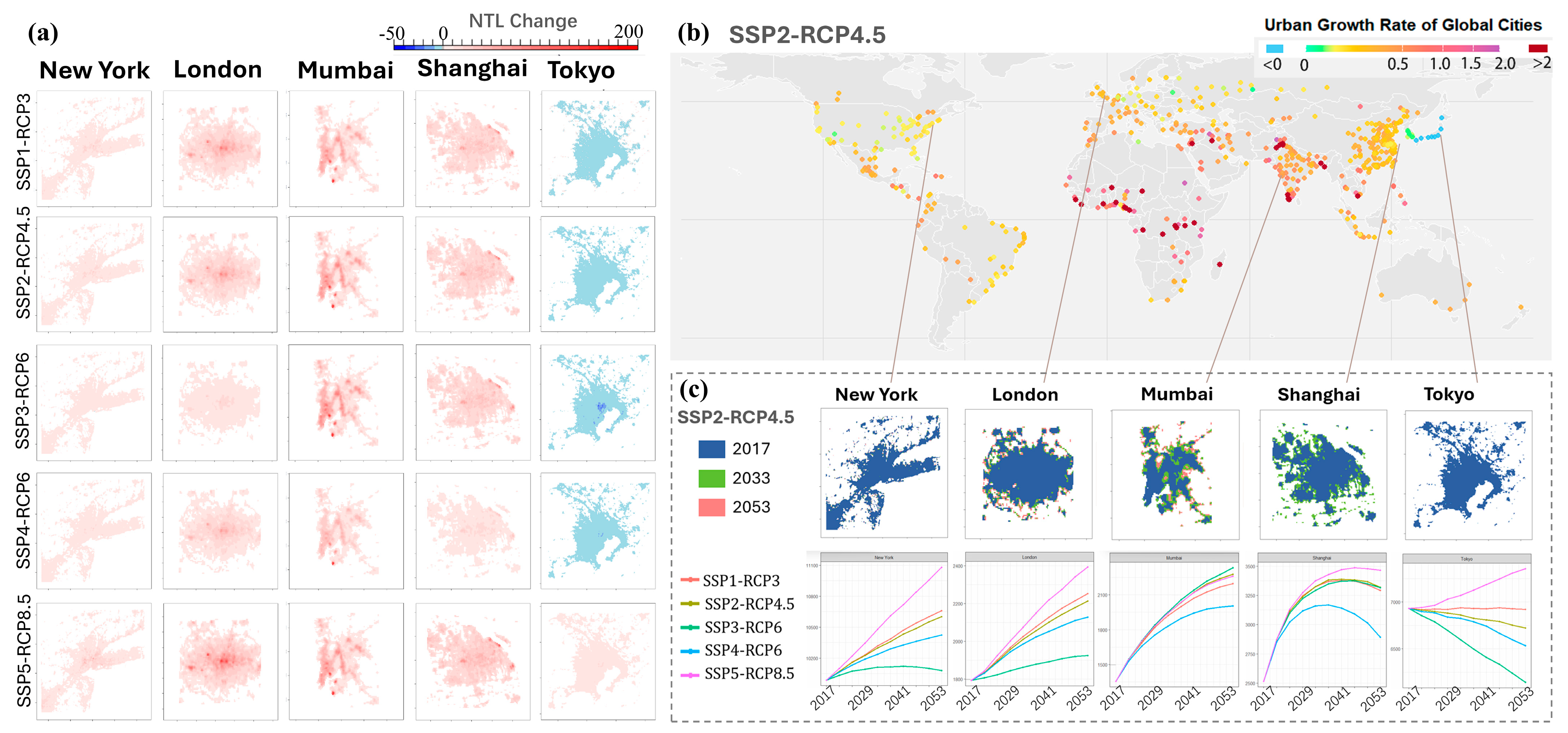
Figure 2a illustrates the spatial patterns of NTL intensity changes between 2017 and 2053 for five representative cities—Tokyo, Shanghai, Mumbai, London, and New York—under all five SSP-RCP scenarios. Red indicates NTL growth, while blue represents decline. The results reveal marked variations across cities and scenarios, highlighting how urban development trajectories are strongly influenced by socioeconomic pathways and policy choices.
Figure 2b presents a global map of projected urban expansion rates between 2017 and 2053 under the SSP2-RCP4.5 scenario. Cities with a negative expansion rate (i.e., shrinkage) are shown in blue. Most cities fall within a 0–2 rate range (i.e., a 0–2-fold increase in urban area) and are rendered in a gradient color scale, while cities with rates exceeding 2 are highlighted in dark red, indicating rapid expansion. It is important to note that this map only visualizes changes for cities included in our 555 samples and does not represent all cities globally.
Figure 2c specifically visualizes the SSP2-RCP4.5 pathway to illustrate its trajectory as the baseline scenario across three time points (2017, 2033, and 2053) in the map. In addition, the trajectories of urban built-up areas of five representative cities are compared from 2017 to 2053 under all five SSP-RCP scenarios.
The results show that NTL intensity exhibits substantial variability across scenarios. Under SSP3-RCP6.0 and SSP4-RCP6.0, the increases in NTL are minimal, suggesting constrained urban growth due to regional fragmentation and limited resources in the former, and pronounced social inequality in the latter. In particular, the effects of these pathways differ by development level. Cities in developed countries experience the most restricted growth under SSP3-RCP6.0, reflecting the impact of reduced international cooperation. Conversely, cities in developing countries are more constrained under SSP4-RCP6.0, where inequality limits access to infrastructure and economic opportunity. In contrast, SSP5-RCP8.5 projects significant NTL increases, indicating accelerated urban expansion under a high-emissions, fossil fuel–dominated development model.
Notably, Tokyo exhibits declining NTL intensity and shrinking urban areas under all scenarios except SSP5-RCP8.5, where a slight increase is observed. Shanghai and Mumbai show rapid expansion before 2033, followed by a slowdown. In particular, under the SSP4-RCP6.0 scenario, Shanghai’s built-up area contracts between 2037 and 2053. These findings suggest that socioeconomic trends and policy frameworks not only influence the extent of urban expansion.
Lastly, as the cities included in our study do not fully represent all urban areas within each country—and the number of sample cities varies by country, the results should not be interpreted as directly characterizing national trends. Instead, they offer insights that may inform urban development policy, while emphasizing the importance of localized, context-specific approaches.

4.2. Projected Urban Expansion and CO2 Emissions of 555 Global Cities

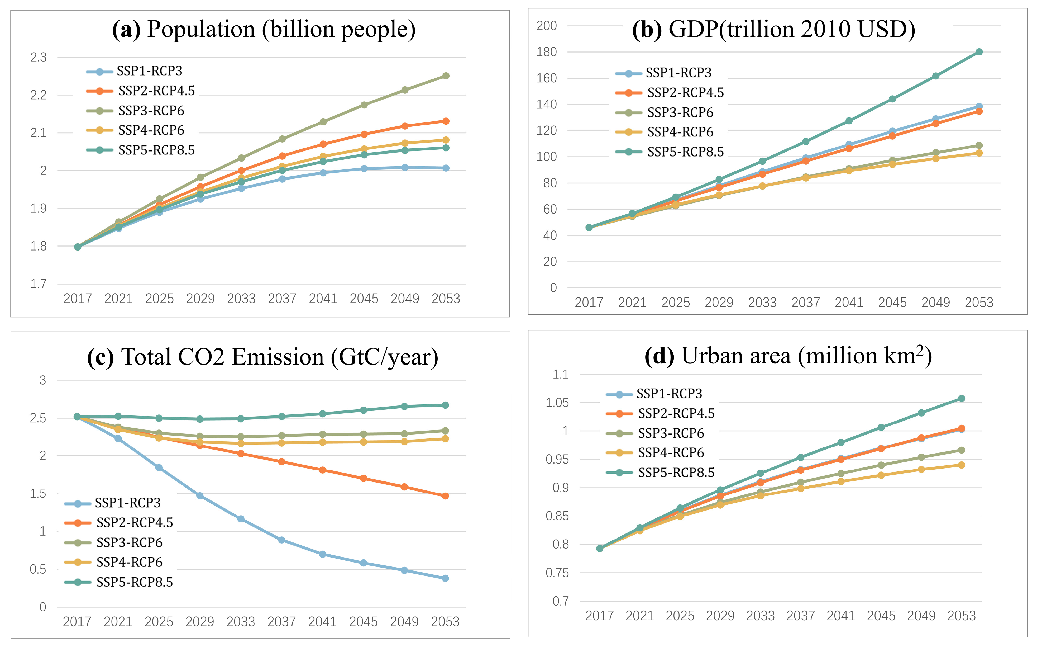
To further understand the macro-level trends of urban development under different socioeconomic trajectories, Figure 3 presents the projected changes in total population, GDP, CO2 emissions, and urban built-up area of 555 target cities under five SSP-RCP scenario combinations. It is important to note that CO2 emissions in this figure are estimated based on the model described in Section 3.3.2, which derives emissions from predicted NTL data, adjusted by a technological improvement factor to account for potential improvements in future energy efficiency under the scenarios.
As shown in Figure 3a,b, urban population and GDP are projected to grow constantly across all scenarios during the target period. The SSP5-RCP8.5 scenario exhibits the strongest momentum in both economic expansion and population growth. In contrast, SSP1-RCP3 and SSP2-RCP4.5 demonstrate more moderate and sustainable development trends, with slower but steadier increases.
Figure 3c presents the projected total CO2 emissions of cities. With the exception of SSP5-RCP8.5, all scenarios exhibit a declining trend in emissions over the coming decades. The most substantial reductions are projected under SSP1-RCP3 and SSP2-RCP4.5. However, this downward trend does not necessarily indicate a real decrease in energy-service demand. Rather, it substantially reflects assumed improvements in energy efficiency and reductions in carbon intensity embedded in the scenario data. This underscores the pivotal role of assumed improvements in energy efficiency and reductions in carbon intensity in achieving urban emission reductions under different scenarios.
Figure 3d displays the projected expansion of built-up urban areas under five SSP-RCP scenarios. Urban land expansion occurs in all scenarios, with the most rapid growth under SSP5-RCP8.5. SSP1-RCP3.4 and SSP2-RCP4.5 follow with nearly overlapping trajectories, while SSP3-RCP6.0 shows slower growth, and SSP4-RCP6.0 exhibits the least expansion. These patterns highlight that while SSP3 and SSP4 assume constrained socioeconomic development and weaker institutional capacity, such conditions suppress urban expansion without achieving substantial emission reductions. In contrast, SSP1 and SSP2 not only moderate land use pressures but also lead to significant reductions in carbon emissions, suggesting that more equitable and sustainability-oriented pathways assume intensive technological progress that promote low-carbon urban development.
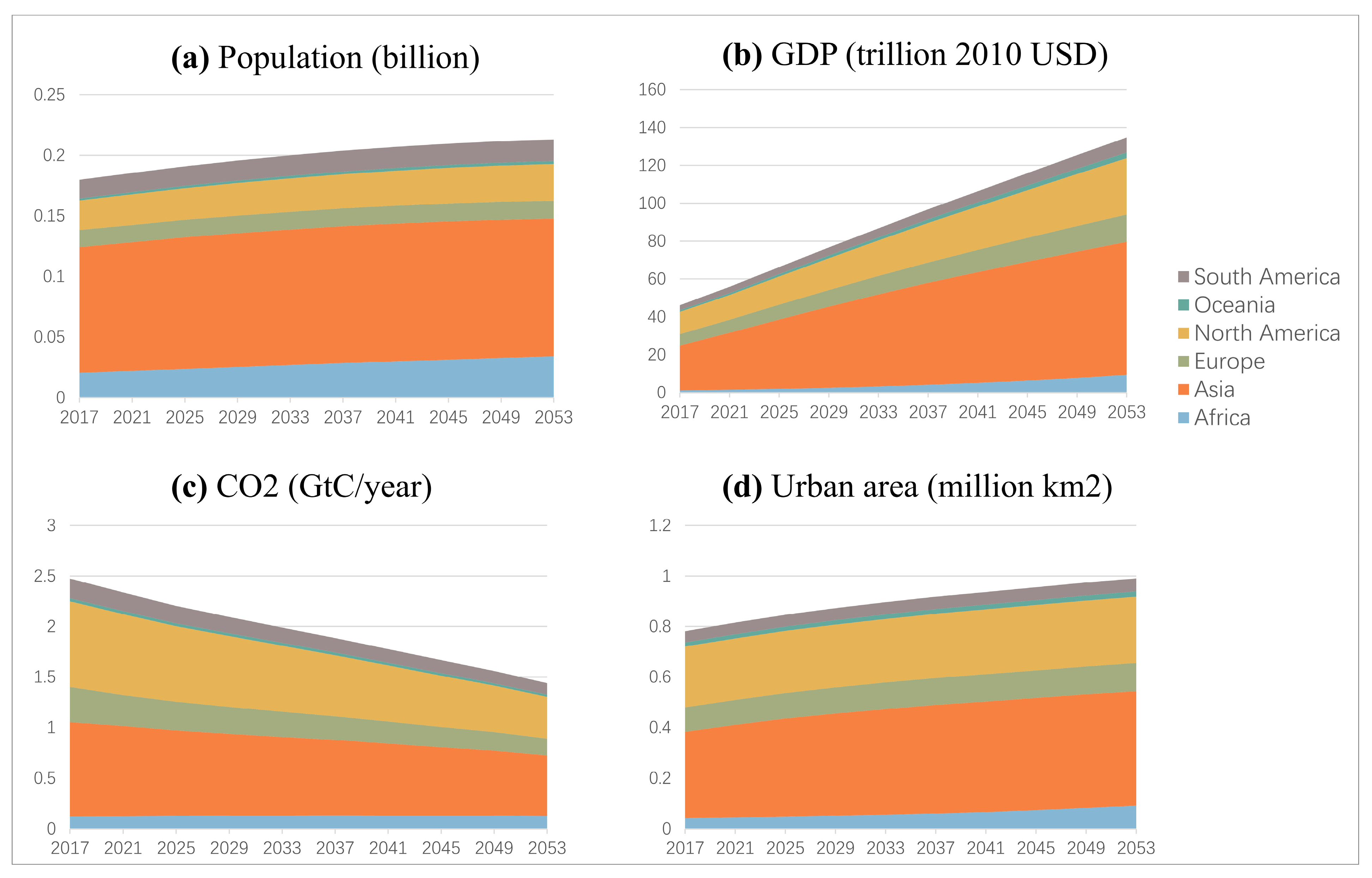
To further explore regional differences, Figure 4 presents the aggregate population, GDP, CO2 emissions, and built-up area expansion of the 555 sample cities across six continents under the SSP2-RCP4.5 scenario. It should be noted again that these results reflect only the sum of the selected cities within each region, rather than the entire global distribution. The prominent contribution of Asian cities is partly due to their greater representation in the dataset. However, this also reflects an underlying demographic and urban reality—Asian cities account for over half of the global urban population and include many of the world’s largest metropolitan areas.
Specifically, Figure 4a,b shows that under SSP2-RCP4.5, Asian cities lead significantly in both population and economic scale, highlighting their sustained urban growth potential. Figure 4c indicates that cities in Asia are also projected to emit the highest total amount of CO2, reflecting the region’s concentrated emission pressure. North America and Europe follow in total emissions; however, North American cities exhibit notably higher per capita CO2 emissions than their Asian counterparts, suggesting a more carbon-intensive urban lifestyle. South America and Oceania contribute relatively less to global emissions. Emissions in Africa are estimated to be almost stable by the middle of this century.
Figure 4d shows that urban built-up area expansion is most prominent in Asian cities, while the highest expansion rates are observed in Africa. These findings underscore the growing importance of urbanization and emissions challenges in developing regions, particularly in Asia and Africa, emphasizing the urgent need for region-specific policy responses and targeted infrastructure investment. Additional regional results for other SSP–RCP scenarios are provided in Supplementary Material S3, which illustrates variations in projected carbon emissions and urban expansion under alternative pathways.

5. Discussion

5.1. Scenario-Based Urban Expansion Trends and Their Policy Implications

The results of our projections highlight the substantial influence of future socioeconomic conditions—captured by population and GDP trajectories under the SSP scenarios—on urban expansion and nighttime light (NTL) dynamics. The heterogeneity observed across cities and scenarios primarily reflects region-specific responses to these drivers, as represented by the random effects in our predictive model. This suggests that future urban growth patterns are shaped not only by overarching global socioeconomic trends but also by inherent regional differences in growth sensitivity
Notably, the limited NTL growth under the SSP3-RCP6.0 scenario—characterized by regional rivalry and weak international cooperation—highlights the restraining effect of fragmented development and constrained technological diffusion on urban intensification. For developing regions, the SSP4-RCP6.0 scenario further reveals how deep socioeconomic inequalities and limited access to advanced technologies become critical barriers to urban growth. Conversely, the pronounced NTL increase under SSP5-RCP8.5, which assumes rapid economic growth fueled by fossil energy, indicates the risk of unchecked urban sprawl and escalating energy demand if mitigation efforts remain insufficient.
The contrasting trends between cities further reflect context-specific dynamics. For instance, Tokyo’s persistent NTL decline and area contraction under most scenarios suggest a maturity-induced stabilization or even shrinkage of highly developed cities under depopulation. This aligns with demographic and economic saturation, aging populations, and policy shifts toward compact urban forms. On the other hand, Shanghai and Mumbai, representing emerging megacities, show continued rapid expansion until around 2033 across scenarios, followed by a slowdown or even contraction in specific cases (e.g., SSP4-RCP6.0). These development trajectories are shaped by direct or indirect socio-economic effects driven by scenario-specific changes in population and economy, and may indicate future saturation thresholds.
Moreover, the selection of SSP2-RCP4.5 as the baseline scenario provides a midpoint reference that neither underestimates growth potential (as in SSP3) nor overstates it (as in SSP5), thus serving as a robust framework for comparative urban studies. The visualized outcomes under this scenario (Figure 2b) also highlight emerging hotspots of urban expansion, particularly in parts of South and Southeast Asia, and sub-Saharan Africa, where ongoing demographic growth and urbanization intersect with limited planning capacity.
These findings carry several implications. First, they underscore the need for differentiated urban strategies that respond not only to national contexts but also to likely future development paths. Second, they emphasize the importance of aligning urban growth with climate mitigation objectives, especially under high-growth, high-emission scenarios. Third, the projections can support early warning systems and guide investment planning by identifying cities at risk of overexpansion or infrastructure strain.
It is also worth noting that our analysis does not explicitly account for the effects of urban policies. While infrastructure development, land use constraints, and governance strategies can shape urban form and NTL dynamics, these factors are only indirectly captured through socioeconomic inputs such as GDP and population and random effect by countries. The localized potential model may partially reflect such influences, but their interpretation requires caution.
Future research should incorporate more explicit policy-related variables—such as zoning regulations, transport infrastructure, and environmental constraints—to refine projections. Integrating indicators of adaptive capacity and urban resilience could further enhance the relevance of NTL-based assessments for understanding quality of life and sustainability.

5.2. Carbon Emission and Spatial Expansion Risks Under Diverging Urbanization Pathways

This section discusses the projected trends of urban expansion and carbon emissions in 555 global cities under varying SSP-RCP scenarios, with a focus on how different development pathways may shape urban sustainability outcomes.
First, the consistent growth in population and GDP across all scenarios confirms the global nature of urban expansion. The SSP5-RCP8.5 scenario shows the most accelerated growth, reflecting a development model driven by high carbon emissions and rapid economic gains. However, this comes at the cost of significant environmental stress and spatial pressure. In contrast, the SSP1-RCP3 and SSP2-RCP4.5 scenarios feature more balanced growth profiles, suggesting stronger potential for sustainable implementation at the urban scale.
Second, while most scenarios exhibit a decline in total urban CO2 emissions over time, it is important to clarify that our model does not directly assume improvements in energy efficiency. Instead, the projected emission reductions are indirectly derived from changes in emission intensity—measured as CO2 emissions per unit of GDP—based on trends provided in the SSP-RCP scenarios. These trends reflect an idealized trajectory of decarbonization driven by various factors, such as advances in energy technologies (including carbon capture and storage), economic restructuring, and changes in consumption patterns. Achieving such reductions in practice, however, requires substantial investment, innovation, and coordinated policy efforts. Our findings underscore that real-world mitigation cannot rely on scenario-driven assumptions alone but must be supported by deep systemic transformations, especially under scenarios where policy action and international coordination are limited.
Moreover, the speed of urban land expansion differs significantly among scenarios. The SSP5-RCP8.5 pathway exhibits the most rapid spatial growth, accompanied by a markedly higher rate of CO2 emissions compared to other pathways. Although this study does not directly assess environmental impacts such as land degradation or ecological stress, the faster emission growth under SSP5-RCP8.5 may imply increased pressure on environmental sustainability if left unmitigated. In particular, several fast-developing regions—including parts of Sub-Saharan Africa and South Asia—show disproportionately high contributions to urban expansion under this scenario, highlighting the need for targeted policy interventions to promote low-carbon and resource-efficient urban development in these areas.
Regionally, the dominant role of Asia and the growing influence of Africa, as shown in Figure 4, underscore the importance of developing countries in shaping future global urban dynamics. Across the five SSP-RCP scenarios, global urban areas are projected to expand by approximately 19–33% by 2053, with particularly rapid growth observed in Asia and Africa. This accelerated expansion will significantly increase demand for infrastructure, services, and broader urban system investments. Furthermore, the anticipated urban growth is expected to contribute to increased CO2 emissions, highlighting the urgent need for sustainable planning and mitigation strategies in rapidly urbanizing regions.
In conclusion, the future trajectory of global urbanization will play a decisive role in shaping carbon emissions, land use patterns, and the overall sustainability of cities. While projected trends suggest opportunities for emissions reductions and balanced growth under certain scenarios, these outcomes are contingent upon ambitious energy efficiency improvements, technological innovation, and structural transformation—none of which are guaranteed. The contrasting dynamics across development pathways and world regions highlight that there is no one-size-fits-all solution. In particular, the pivotal role of Asia and the rising urban momentum in Africa call for targeted, region-specific strategies that align infrastructure investments, policy design, and institutional capacity with sustainable urban goals. Guiding cities toward more compact, low-carbon, and resilient forms will require not only foresight, but also sustained political commitment and global cooperation.

5.3. Limitations and Directions for Future Research

Although this study has systematically advanced the integration of multi-scale remote sensing and socio-economic data for predicting future urban NTL intensity and carbon emissions, several limitations remain and merit further improvement and expansion.

5.3.1. Model Structure and Theoretical Simplifications

First, our modeling approach assumes population and GDP per capita as exogenous drivers of urban expansion. However, as raised in the literature, the relationship is likely characterized by bidirectional causality: urban expansion can also foster economic growth and attract population influx. This endogeneity concern means that the estimated coefficients in our macro-level model should be interpreted as capturing strong predictive associations rather than isolated causal effects. This limitation is inherent to many large-scale, prognostic studies that rely on integrated assessment model outputs like the SSPs, where the focus is on consistent scenario projection rather than on disentangling causal mechanisms. While our use of mixed-effects models controls for time-invariant national characteristics, future research aimed at causal inference could benefit from employing instrumental variable techniques or natural experiments, albeit at a more localized scale where such instruments are identifiable.
Second, the technological adjustment factor (δ) introduced in this study provides a simplified and idealized means of reflecting long-term improvements in carbon emission efficiency. It is conceptually rooted in the Kaya Identity and partially compensates for the model’s inability—based solely on the relationship between NTL and carbon emissions per unit area—to capture future changes in energy efficiency. However, this approach does not explicitly model the distinct impacts of other critical drivers of urban carbon trajectories, such as shifts in the energy mix, policy interventions, or sectoral economic shifts, which are only implicitly aggregated within the national CO2/GDP ratios from the SSP-RCP scenarios. Furthermore, the factor applies a uniform national-level trend to all grids within a country, which does not capture potential spatial heterogeneity in the adoption of low-carbon technologies within individual cities. While this adjustment enhances projected emission reductions and ensures consistency with national scenario pathways, future research should refine this mechanism by developing a more detailed and dynamic framework of influencing factors, potentially incorporating energy system simulations, policy scenario modeling, and intra-urban technology diffusion patterns to improve the contextual accuracy and adaptability of long-term carbon emission projections.
Third, the grid-level potential model demonstrated strong predictive performance in out-of-sample validation, particularly after excluding non-urban outliers (test R2 = 0.951). This result underscores the model’s ability to capture typical urban development patterns. However, the presence of outliers—such as military facilities with extreme NTL values—can substantially influence performance metrics if not accounted for. The interpretative focus should therefore be on the fixed effects, which represent global trends, and the variance components of the random effects, which quantify the magnitude of inter-city differences. Readers are cautioned that the model’s performance is contingent on the representativeness of the input data and that predictions for atypical areas (e.g., high-intensity non-urban sites) should be interpreted with care.

5.3.2. Spatial and Temporal Limitations

In the spatial visualizations of projected NTL and carbon emissions, certain non-core urban areas exhibit pronounced emission hotspots. These regions display unusually high NTL intensity and predicted emission values compared to their surroundings. Cross-validation with satellite imagery and geographic maps reveals that most of these hotspots correspond to major industrial complexes, airports, and other facilities with intensive nighttime lighting demand. As noted in Section 3.4.2, the inclusion of these outliers significantly reduces the apparent predictive performance of the model (test R2 drops from 0.951 to 0.556 when such sites are included). This indicates that the model, while capturing general urban dynamics effectively, may not fully represent the patterns of these atypical, high-intensity sites. As this study did not exclude or independently model such facilities, the resulting projections should be interpreted with caution in these contexts. Future research should consider incorporating spatial data on industrial and transportation infrastructure to annotate, exclude, or separately model these areas, thereby improving the socio-economic interpretability and predictive accuracy of the models.
In addition, while the rank-based allocation method is built on a theoretical foundation of urban path dependence, its empirical validation across a wider range of urban contexts and over longer time periods would strengthen its generalizability. Future research could employ multi-temporal urban form data to explicitly test the stability of intra-urban development rankings and refine the matching algorithm.

5.3.3. Scaling and Representation Constraints

Furthermore, our model applies national-level socioeconomic growth rates (for GDP and population) from the SSP-RCP scenarios uniformly to all cities within a country. This approach, while necessary to ensure the projected urban system maintains a city-size distribution consistent with empirically observed patterns (e.g., Zipf’s law) at the national scale [59,60], does not capture heterogeneous growth dynamics among individual cities. In reality, urban growth rates are influenced by local policies, geographical constraints, economic specialization, and agglomeration effects, which can lead to significant divergence between the growth of primate cities or specific regions and the national average. Consequently, while our model provides robust projections of aggregate urban expansion and emissions, its predictions for the trajectory of any specific city should be interpreted with caution. Future studies could refine this aspect by incorporating subnational socioeconomic projections or modeling internal migration patterns where reliable data are available, and, in the longer term, extending these approaches to global-scale studies as harmonized datasets become accessible.
Lastly, the modeling approach in this study is based on historical data that capture country-level trends in urban expansion and emissions. As such, the derived urban growth patterns reflect a static trajectory assuming the continuation of existing development paths. However, urban expansion is subject to dynamic influences including policy changes, global economic shifts, and technological breakthroughs. Changes in national or regional development strategies may substantially alter future urbanization and emission outcomes. To improve model responsiveness to such uncertainties, future work should incorporate dynamic parameters or scenario-based policy adjustments, enabling better alignment with diverse regional development trajectories and enhancing the realism of future urban projections. Moreover, it is important to note that the cities selected for this study do not cover all urban areas within each country, and the number of sampled cities varies across nations. As such, the results should not be interpreted as representative of national characteristics in a strict sense, but rather as indicative patterns for reference. Policymaking should be adapted to local contexts accordingly.

6. Conclusions

This study proposes an integrated modeling framework to simulate future urban nighttime light (NTL) intensity, urban expansion and CO2 emissions at high spatial resolution by combining remote sensing data with socioeconomic variables under SSP–RCP scenarios. A key methodological contribution lies in the use of multi-level linear mixed-effects models, which capture spatial heterogeneity across countries and cities by distinguishing national development patterns from local urban dynamics. The introduction of a technological adjustment factor further enhances the emission model by accounting for efficiency improvements, while the use of SSP–RCP combinations instead of single scenarios offers a more nuanced reflection of future uncertainties in development and climate policies.
The simulation results for 555 global cities from 2017 to 2053 reveal notable differences in urban expansion mechanisms: economic growth drives NTL increases in many Asian cities, while population pressure dominates in parts of Africa and Latin America. Mature cities in high-income countries show signs of spatial saturation and emission decoupling. These patterns underline the need for locally adapted planning strategies.
Scenario-based projections highlight how divergent global development pathways can reshape urban forms and sustainability outcomes. High-growth scenarios (e.g., SSP5–RCP8.5) indicate rapid NTL expansion, implying increased energy demand and environmental stress. In contrast, more sustainable pathways constrain sprawl but pose challenges in avoiding stagnation or inequality. While projected CO2 emissions generally decline due to assumed efficiency gains, the reliance on idealized parameters calls for further empirical validation.
Overall, this study contributes a scalable, data-driven tool for anticipating future urban and carbon dynamics. By leveraging globally available NTL data and basic socioeconomic indicators, the approach is particularly well-suited for application in data-scarce regions, enabling consistent assessments across diverse urban contexts. It offers actionable insights for planners and policymakers seeking to balance development and climate goals. Future research should incorporate institutional, land-use, and resilience dimensions, and further advance dynamic modeling frameworks to support adaptive and equitable urban sustainability strategies.

Supplementary Materials

The following supporting information can be downloaded at: https://www.mdpi.com/article/10.3390/rs17183251/s1, S1: Clustering Analysis of Country-Level NTL Sensitivities. S2: Temporal Evolution of Scenario-Based Energy Efficiency Correction Factors. S3: Regional aggregates of estimated urban area and carbon emissions under multiple SSP–RCP scenarios. S4. Detailed Procedure for Adjusting the India-Specific GDP Coefficient. S5. Residual Analysis and Model Diagnostics.

Author Contributions

Conceptualization, M.K. and J.X.; methodology, M.K. and J.X.; software, J.X., Y.O. and M.K.; validation, J.X., Y.O. and M.K.; formal analysis, J.X., Y.O. and M.K.; investigation, J.X., Y.O. and M.K.; resources, J.X., Y.O. and M.K.; data curation, J.X., Y.O. and M.K.; writing—original draft preparation, J.X., C.-C.C. and M.K.; writing—review and editing, J.X., C.-C.C. and M.K.; visualization, J.X.; supervision, M.K. and C.-C.C.; project administration, M.K.; funding acquisition, M.K. All authors have read and agreed to the published version of the manuscript.

Funding

This research was funded by the Japan Science and Technology Agency (JST) as part of SICORP [grant number JPMJSC22E2].

Data Availability Statement

All the data used in this study are available from the cited references. In addition, we provide the estimated future nighttime light data for all 555 target cities in GeoTIFF format, organized by year and scenario, at [https://see.eng.osaka-u.ac.jp/seeud/seeud/data/xu_2501/datashare0810.html, accessed on 20 August 2025].

Acknowledgments

We appreciate the anonymous reviewers for their invaluable comments made to improve the manuscript. Needless to say, any errors or inaccuracies are the responsibility of the authors.

Conflicts of Interest

The authors declare no conflicts of interest. The funders had no role in the design of the study; in the collection, analyses, or interpretation of data; in the writing of the manuscript, or in the decision to publish the results.

References

  1. United Nations Human Settlements Programme (UN-Habitat). World Cities Report 2022: Envisaging the Future of Cities; UN-Habitat: Nairobi, Kenya, 2022. [Google Scholar]
  2. Krayenhoff, E.S.; Moustaoui, M.; Broadbent, A.M.; Gupta, V.; Georgescu, M. Diurnal interaction between urban expansion, climate change and adaptation in US cities. Nat. Clim. Change 2018, 8, 1097–1103. [Google Scholar] [CrossRef]
  3. Liu, F.; Zhang, Z.; Zhao, X.; Wang, X.; Zuo, L.; Wen, Q.; Yi, L.; Xu, J.; Hu, S.; Liu, B. Chinese cropland losses due to urban expansion in the past four decades. Sci. Total Environ. 2019, 650, 847–857. [Google Scholar] [CrossRef] [PubMed]
  4. Liu, W.; Zhan, J.; Zhao, F.; Yan, H.; Zhang, F.; Wei, X. Impacts of urbanization-induced land-use changes on ecosystem services: A case study of the Pearl River Delta Metropolitan Region, China. Ecol. Indic. 2019, 98, 228–238. [Google Scholar] [CrossRef]
  5. Seto, K.C.; Fragkias, M.; Güneralp, B.; Reilly, M.K. A meta-analysis of global urban land expansion. PLoS ONE 2011, 6, e23777. [Google Scholar] [CrossRef] [PubMed]
  6. Seto, K.C.; Güneralp, B.; Hutyra, L.R. Global forecasts of urban expansion to 2030 and direct impacts on biodiversity and carbon pools. Proc. Natl. Acad. Sci. USA 2012, 109, 16083–16088. [Google Scholar] [CrossRef] [PubMed]
  7. Zhang, Z.; Liu, F.; Zhao, X.; Wang, X.; Shi, L.; Xu, J.; Yu, S.; Wen, Q.; Zuo, L.; Yi, L. Urban expansion in China based on remote sensing technology: A review. Chin. Geogr. Sci. 2018, 28, 727–743. [Google Scholar] [CrossRef]
  8. Poelmans, L.; Van Rompaey, A. Complexity and performance of urban expansion models. Comput. Environ. Urban Syst. 2010, 34, 17–27. [Google Scholar] [CrossRef]
  9. Din, S.U.; Yamamoto, K. Urban spatial dynamics and geo-informatics prediction of Karachi from 1990–2050 using remote sensing and CA-ANN simulation. Earth Syst. Environ. 2024, 8, 849–868. [Google Scholar] [CrossRef]
  10. Wu, Y.; Li, C.; Shi, K.; Liu, S.; Chang, Z. Exploring the effect of urban sprawl on carbon dioxide emissions: An urban sprawl model analysis from remotely sensed nighttime light data. Environ. Impact Assess. Rev. 2022, 93, 106731. [Google Scholar] [CrossRef]
  11. Duan, X.; Hu, Q.; Zhao, P.; Wang, S.; Ai, M. An approach of identifying and extracting urban commercial areas using the nighttime lights satellite imagery. Remote Sens. 2020, 12, 1029. [Google Scholar] [CrossRef]
  12. Tong, L.; Hu, S.; Frazier, A.E. Mixed accuracy of nighttime lights (NTL)-based urban land identification using thresholds: Evidence from a hierarchical analysis in Wuhan Metropolis, China. Appl. Geogr. 2018, 98, 201–214. [Google Scholar] [CrossRef]
  13. Liu, H.; Luo, N.; Hu, C. Detection of county economic development using LJ1-01 nighttime light imagery: A comparison with NPP-VIIRS data. Sensors 2020, 20, 6633. [Google Scholar] [CrossRef]
  14. Wan, W.; Chen, H.; Yang, X.; Li, R.; Cui, Y.; Hu, Y. Identifying the Hierarchical Structure of Nighttime Economic Agglomerations Based on the Fusion of Multisource Data. ISPRS Int. J. Geo-Inf. 2024, 13, 188. [Google Scholar] [CrossRef]
  15. Wu, J.; Tu, Y.; Chen, Z.; Yu, B. Analyzing the Spatially Heterogeneous Relationships between Nighttime Light Intensity and Human Activities across Chongqing, China. Remote Sens. 2022, 14, 5695. [Google Scholar] [CrossRef]
  16. Liu, B.; Lv, J. Spatiotemporal Evolution and Tapio Decoupling Analysis of Energy-Related Carbon Emissions Using Nighttime Light Data: A Quantitative Case Study at the City Scale in Northeast China. Energies 2024, 17, 4795. [Google Scholar] [CrossRef]
  17. Kii, M.; Matsumoto, K.; Sugita, S. Future Scenarios of Urban Nighttime Lights: A Method for Global Cities and Its Application to Urban Expansion and Carbon Emission Estimation. Remote Sens. 2024, 16, 1018. [Google Scholar] [CrossRef]
  18. Laird, N.M.; Ware, J.H. Random-effects models for longitudinal data. Biometrics 1982, 38, 963–974. [Google Scholar] [CrossRef] [PubMed]
  19. Van Vuuren, D.P.; Kriegler, E.; O’Neill, B.C.; Ebi, K.L.; Riahi, K.; Carter, T.R.; Edmonds, J.; Hallegatte, S.; Kram, T.; Mathur, R. A new scenario framework for climate change research: Scenario matrix architecture. Clim. Change 2014, 122, 373–386. [Google Scholar] [CrossRef]
  20. Angel, S.; Parent, J.; Civco, D.L.; Blei, A.; Potere, D. The dimensions of global urban expansion: Estimates and projections for all countries, 2000–2050. Prog. Plan. 2011, 75, 53–107. [Google Scholar] [CrossRef]
  21. Gao, C.; Feng, Y.; Tong, X.; Lei, Z.; Chen, S.; Zhai, S. Modeling urban growth using spatially heterogeneous cellular automata models: Comparison of spatial lag, spatial error and GWR. Comput. Environ. Urban Syst. 2020, 81, 101459. [Google Scholar] [CrossRef]
  22. Huang, B.; Xie, C.; Tay, R. Support vector machines for urban growth modeling. Geoinformatica 2010, 14, 83–99. [Google Scholar] [CrossRef]
  23. Mohammady, S.; Delavar, M.R. Urban sprawl assessment and modeling using landsat images and GIS. Model. Earth Syst. Environ. 2016, 2, 155. [Google Scholar] [CrossRef]
  24. Mozaffaree Pour, N.; Oja, T. Prediction Power of Logistic Regression (LR) and Multi-Layer Perceptron (MLP) Models in Exploring Driving Forces of Urban Expansion to Be Sustainable in Estonia. Sustainability 2022, 14, 160. [Google Scholar] [CrossRef]
  25. Rana, M.S.; Sarkar, S. Prediction of urban expansion by using land cover change detection approach. Heliyon 2021, 7, e08437. [Google Scholar] [CrossRef] [PubMed]
  26. Al-shalabi, M.; Billa, L.; Pradhan, B.; Mansor, S.; Al-Sharif, A.A. Modelling urban growth evolution and land-use changes using GIS based cellular automata and SLEUTH models: The case of Sana’a metropolitan city, Yemen. Environ. Earth Sci. 2013, 70, 425–437. [Google Scholar] [CrossRef]
  27. Boulila, W.; Ghandorh, H.; Khan, M.A.; Ahmed, F.; Ahmad, J. A novel CNN-LSTM-based approach to predict urban expansion. Ecol. Inform. 2021, 64, 101325. [Google Scholar] [CrossRef]
  28. Chettry, V.; Surawar, M. Delineating urban growth boundary using remote sensing, ANN-MLP and CA model: A case study of Thiruvananthapuram urban agglomeration, India. J. Indian Soc. Remote Sens. 2021, 49, 2437–2450. [Google Scholar] [CrossRef]
  29. Liu, X.; Liang, X.; Li, X.; Xu, X.; Ou, J.; Chen, Y.; Li, S.; Wang, S.; Pei, F. A future land use simulation model (FLUS) for simulating multiple land use scenarios by coupling human and natural effects. Landsc. Urban Plan. 2017, 168, 94–116. [Google Scholar] [CrossRef]
  30. Gao, J.; O’Neill, B.C. Mapping global urban land for the 21st century with data-driven simulations and Shared Socioeconomic Pathways. Nat. Commun. 2020, 11, 2302. [Google Scholar] [CrossRef]
  31. Chen, G.; Li, X.; Liu, X.; Chen, Y.; Liang, X.; Leng, J.; Xu, X.; Liao, W.; Qiu, Y.; Wu, Q. Global projections of future urban land expansion under shared socioeconomic pathways. Nat. Commun. 2020, 11, 537. [Google Scholar] [CrossRef]
  32. Hansen, M.C.; Loveland, T.R. A review of large area monitoring of land cover change using Landsat data. Remote Sens. Environ. 2012, 122, 66–74. [Google Scholar] [CrossRef]
  33. Mertes, C.M.; Schneider, A.; Sulla-Menashe, D.; Tatem, A.; Tan, B. Detecting change in urban areas at continental scales with MODIS data. Remote Sens. Environ. 2015, 158, 331–347. [Google Scholar] [CrossRef]
  34. Matci, D.K. Development of a new index for mapping urban areas in Türkiye using Sentinel-2 images. Adv. Space Res. 2023, 72, 4677–4691. [Google Scholar] [CrossRef]
  35. Bagan, H.; Yamagata, Y. Analysis of urban growth and estimating population density using satellite images of nighttime lights and land-use and population data. GISci. Remote Sens. 2015, 52, 765–780. [Google Scholar] [CrossRef]
  36. Li, S.; Dragicevic, S.; Castro, F.A.; Sester, M.; Winter, S.; Coltekin, A.; Pettit, C.; Jiang, B.; Haworth, J.; Stein, A. Geospatial big data handling theory and methods: A review and research challenges. ISPRS J. Photogramm. Remote Sens. 2016, 115, 119–133. [Google Scholar] [CrossRef]
  37. Zhang, Q.; Schaaf, C.; Seto, K.C. The vegetation adjusted NTL urban index: A new approach to reduce saturation and increase variation in nighttime luminosity. Remote Sens. Environ. 2013, 129, 32–41. [Google Scholar] [CrossRef]
  38. He, X.; Zhang, Z.; Yang, Z. Extraction of urban built-up area based on the fusion of night-time light data and point of interest data. R. Soc. Open Sci. 2021, 8, 210838. [Google Scholar] [CrossRef]
  39. Kii, M.; Tamaki, T.; Suzuki, T.; Nonomura, A. Estimating urban spatial structure based on remote sensing data. Sci. Rep. 2023, 13, 8804. [Google Scholar] [CrossRef]
  40. Xin, X.; Liu, B.; Di, K.; Zhu, Z.; Zhao, Z.; Liu, J.; Yue, Z.; Zhang, G. Monitoring urban expansion using time series of night-time light data: A case study in Wuhan, China. In Remote Sensing of Night-Time Light; Routledge: London, UK, 2021; pp. 256–274. [Google Scholar]
  41. Liu, Z.; He, C.; Zhang, Q.; Huang, Q.; Yang, Y. Extracting the dynamics of urban expansion in China using DMSP-OLS nighttime light data from 1992 to 2008. Landsc. Urban Plan. 2012, 106, 62–72. [Google Scholar] [CrossRef]
  42. Kii, M.; Matsumoto, K. Detecting Urban Sprawl through Nighttime Light Changes. Sustainability 2023, 15, 16506. [Google Scholar] [CrossRef]
  43. Xiao, P.; Wang, X.; Feng, X.; Zhang, X.; Yang, Y. Detecting China’s urban expansion over the past three decades using nighttime light data. IEEE J. Sel. Top. Appl. Earth Obs. Remote Sens. 2014, 7, 4095–4106. [Google Scholar] [CrossRef]
  44. Moran, D.; Kanemoto, K.; Jiborn, M.; Wood, R.; Többen, J.; Seto, K.C. Carbon footprints of 13,000 cities. Environ. Res. Lett. 2018, 13, 064041. [Google Scholar] [CrossRef]
  45. Wang, G.; Han, Q.; de Vries, B. A geographic carbon emission estimating framework on the city scale. J. Clean. Prod. 2020, 244, 118793. [Google Scholar] [CrossRef]
  46. Fang, G.; Gao, Z.; Tian, L.; Fu, M. What drives urban carbon emission efficiency?—Spatial analysis based on nighttime light data. Appl. Energy 2022, 312, 118772. [Google Scholar] [CrossRef]
  47. Song, M.; Wang, Y.; Han, Y.; Ji, Y. Estimation Model and Spatio-Temporal Analysis of Carbon Emissions from Energy Consumption with NPP-VIIRS-like Nighttime Light Images: A Case Study in the Pearl River Delta Urban Agglomeration of China. Remote Sens. 2024, 16, 3407. [Google Scholar] [CrossRef]
  48. Jin, Y.; Sharifi, A.; Li, Z.; Chen, S.; Zeng, S.; Zhao, S. Carbon emission prediction models: A review. Sci. Total Environ. 2024, 927, 172319. [Google Scholar] [CrossRef]
  49. O’neill, B.C.; Dalton, M.; Fuchs, R.; Jiang, L.; Pachauri, S.; Zigova, K. Global demographic trends and future carbon emissions. Proc. Natl. Acad. Sci. USA 2010, 107, 17521–17526. [Google Scholar] [CrossRef]
  50. Gurney, K.R.; Kılkış, Ş.; Seto, K.C.; Lwasa, S.; Moran, D.; Riahi, K.; Keller, M.; Rayner, P.; Luqman, M. Greenhouse gas emissions from global cities under SSP/RCP scenarios, 1990 to 2100. Glob. Environ. Change 2022, 73, 102478. [Google Scholar] [CrossRef]
  51. Gütschow, J.; Jeffery, M.L.; Günther, A.; Meinshausen, M. Country-resolved combined emission and socio-economic pathways based on the Representative Concentration Pathway (RCP) and Shared Socio-Economic Pathway (SSP) scenarios. Earth Syst. Sci. Data 2021, 13, 1005–1040. [Google Scholar] [CrossRef]
  52. Kummu, M.; Taka, M.; Guillaume, J.H. Gridded global datasets for gross domestic product and human development index over 1990–2015. Sci. Data 2018, 5, 180004. [Google Scholar] [CrossRef]
  53. Elvidge, C.D.; Zhizhin, M.; Ghosh, T.; Hsu, F.-C.; Taneja, J. Annual time series of global VIIRS nighttime lights derived from monthly averages: 2012 to 2019. Remote Sens. 2021, 13, 922. [Google Scholar] [CrossRef]
  54. Oda, T.; Maksyutov, S. A very high-resolution (1 km× 1 km) global fossil fuel CO2 emission inventory derived using a point source database and satellite observations of nighttime lights. Atmos. Chem. Phys. 2011, 11, 543–556. [Google Scholar] [CrossRef]
  55. Oda, T.; Maksyutov, S.; Andres, R.J. The Open-source Data Inventory for Anthropogenic Carbon dioxide (CO2), version 1 2016 (ODIAC2016): A global, monthly fossil-fuel CO2 gridded emission data product for 2 tracer transport simulations and surface flux inversions 3. Earth Syst. Sci. Data 2018, 10, 87–107. [Google Scholar] [CrossRef]
  56. ESA. Land Cover CCI Product User Guide Version 2; European Space Agency: Brussels, Belgium, 2017; p. 105. [Google Scholar]
  57. Kaya, Y. Impact of Carbon Dioxide Emission Control on GNP Growth: Interpretation of Proposed Scenarios; Intergovernmental Panel on Climate Change/Response Strategies Working Group (IPCC): Geneva, Switzerland, 1989. [Google Scholar]
  58. Lee, K.; Yun, S.-J.; Park, S. Varied drivers for reducing CO2 emissions in countries with legislated carbon neutrality targets: A Kaya identity clustering analysis. Environ. Dev. Sustain. 2025, 1–23. [Google Scholar] [CrossRef]
  59. Kii, M.; Akimoto, K.; Doi, K. Random-growth urban model with geographical fitness. Phys. A Stat. Mech. Its Appl. 2012, 391, 5960–5970. [Google Scholar] [CrossRef]
  60. Kii, M. Projecting future populations of urban agglomerations around the world and through the 21st century. Npj Urban Sustain. 2021, 1, 10. [Google Scholar] [CrossRef]
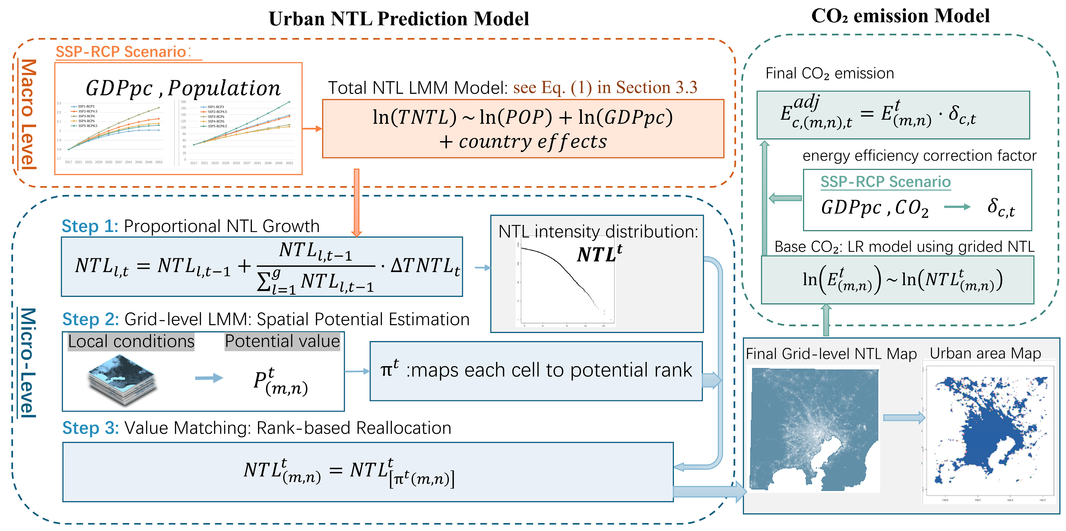
Figure 1. Analytical Framework.
Remotesensing 17 03251 g001
Figure 2. Projected Urban Expansion and Nighttime Light (NTL) Changes in 555 Cities Under Five SSP–RCP Scenarios (2017–2053). (a) Spatial distribution of projected NTL intensity changes for five representative cities—New York, London, Mumbai, Shanghai, and Tokyo—under five SSP–RCP scenarios. In (a), red indicates growth in NTL, while blue indicates decline. (b) Global distribution of projected urban expansion rates for 555 cities under the SSP2–RCP4.5 scenario. In (b), cities with a negative growth rate (shrinkage) are shown in blue; those with a rate above 2 are highlighted in dark red. (c) Comparison of built-up area changes for the five selected cities at three time points (2017, 2033, and 2053) under the SSP2–RCP4.5 scenario. Additionally, urban area changes from 2017–2053 under all five SSP–RCP scenarios are visualized.
Remotesensing 17 03251 g002
Figure 3. Population and GDP projections derived from SSP–RCP scenarios, and estimated CO2 emissions and urban expansion for 555 cities under different SSP–RCP pathways: (a) population, (b) GDP, (c) CO2 emissions, and (d) urban areas.
Remotesensing 17 03251 g003
Figure 4. Regional aggregates of population, GDP scenarios, and estimated urban area and carbon emissions under the SSP2 scenario: (a) population, (b) GDP, and (c) carbon emissions, (d) urban area.
Remotesensing 17 03251 g004
Table 1. Estimation Results of Fixed and Random Effects in the Mixed Effects Model.
Fixed EffectsEstimatet-ValueRandom EffectsStd. Dev.
β 0 −2.941−5.261 u 0 , c 3.358
β 1 0.841319.865 u 1 , c 0.2412
β 2 0.597310.513 u 2 , c 0.3278
ε 1 0.5019
Number of samples1665
groups109
Conditional R20.8496
Table 2. Fixed and random effect estimates of the selected grid-level potential model.
Variable NameDescriptionFixed Effects
(Estimate)
Fixed Effects
(t-Value)
Random Effects (Std. Dev.)
p N T L t 1 Nighttime light intensity in the previous year 0.8294 139.543 0.1349
R T C Road travel time to city center 0.7693 −4.335 4.065
R D D Distance to nearest road 1.549 × 10 4 −5.620 6.495 × 10 4
P T C Railway travel time to city center 0.1102 −1.468 1.787
t s l p . s d Standard deviation of slope 6.214 −23.932 4.351
P R C Maximum daily precipitation 4.176 × 10 2 −0.244 2.986
N T L f c t 1 Focal total NTL from 8 surrounding cells in year t − 1 0.1965 30.087 0.1452
T M P a Annual average temperature 2.355 × 10 3 −0.771
T M P v Annual temperature variability (standard deviation) 5.116 × 10 4 −4.382
P R C a Annual average precipitation 1.032 × 10 4 4.468
P O P t Population density of agglomeration 6.003 × 10 5 2.211
G D P p c t Per capita GDP of agglomeration 4.029 × 10 6 −0.802
I n t e r c e p t Intercept 2.047 8.401 4.014
ε 2 t Residual 3.501
Number of samples 2,555,832
groups 571
Train R20.579test R20.566
Disclaimer/Publisher’s Note: The statements, opinions and data contained in all publications are solely those of the individual author(s) and contributor(s) and not of MDPI and/or the editor(s). MDPI and/or the editor(s) disclaim responsibility for any injury to people or property resulting from any ideas, methods, instructions or products referred to in the content.