Article

Fine-Scale Mapping and Uncertainty Quantification of Intertidal Sediment Grain Size Using Geostatistical Simulation Integrated with Machine Learning and High-Resolution Remote Sensing Imagery

by
No-Wook Park
1,* and
Dong-Ho Jang
2
1
Department of Geoinformatic Enginnering, Inha University, Incheon 22212, Republic of Korea
2
Department of Geography, Kongju National University, Gongju 32588, Republic of Korea
*
Author to whom correspondence should be addressed.
Remote Sens. 2025, 17(18), 3230; https://doi.org/10.3390/rs17183230
Submission received: 28 July 2025 / Revised: 15 September 2025 / Accepted: 18 September 2025 / Published: 18 September 2025
(This article belongs to the Section Environmental Remote Sensing)

Abstract

Highlights

What are the main findings?
  • Incorporating satellite-derived features into the random forest model improved the accuracy of grain size prediction compared to using field samples alone.
  • The proposed geostatistical simulation framework enabled explicit quantification of prediction uncertainty.
What is the implication of the main finding?
  • Satellite-derived features, when integrated with machine learning and multivariate geostatistics, can be used to complement limited field data in tidal flats.
  • The proposed approach provides fine-scale grain-size maps with associated uncertainty information to support coastal management.

Abstract

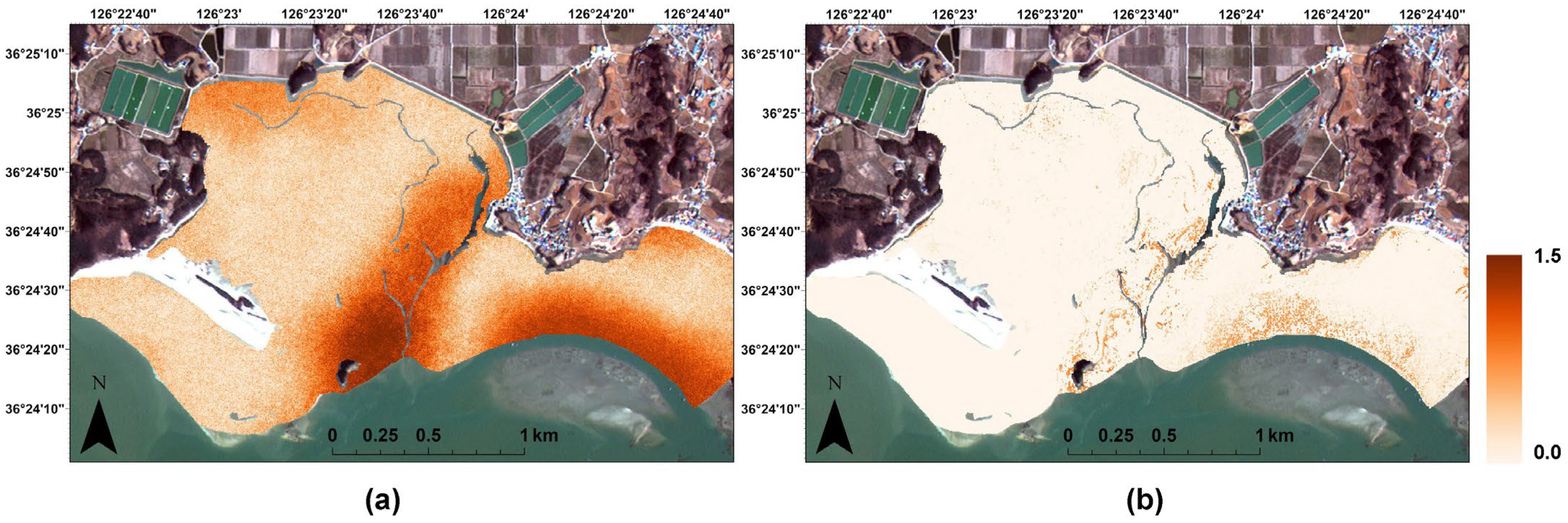
This study presents a geostatistical simulation approach for fine-scale grain size mapping in tidal flats, which complements sparse field survey data with high-resolution optical satellite imagery and quantifies prediction uncertainty at unsampled locations. Within a multi-Gaussian regression kriging (MGRK) framework, a random forest (RF) regression model is used to estimate the trend component of grain size variability in Gaussian space. Residual components are estimated using kriging, and the trend and residual components are combined to construct conditional cumulative distribution functions for uncertainty modeling. Sequential Gaussian simulation based on the CCDFs generates alternative realizations of grain size, allowing for quantification of prediction uncertainty. The potential of this integrated approach was tested on the Baramarae tidal flat in Korea using KOMPSAT-2 imagery. Three spectral features, the green band, red band, and normalized difference water index (NDWI), explained 42.74% of the grain size variability, with NDWI identified as the most influential feature, contributing 40.8% compared with 31.7% for the red band and 27.5% for the green band. MGRK effectively captured local grain size variations, reducing the mean absolute error from 0.554 to 0.280 compared with univariate kriging based solely on field survey data, corresponding to an improvement of approximately 49.5%. The benefit of the proposed approach was validated by a reduction in prediction uncertainty, with the mean standard deviation decreasing from 0.743 in simulations based solely on field data to 0.280 in MGRK-based simulations. These findings indicate that the proposed geostatistical approach, integrating satellite-derived features, is a reliable method for fine-scale mapping of intertidal sediment grain size by providing both predictions and associated uncertainty estimates.

Graphical Abstract

1. Introduction

Tidal flats, formed by the deposition of sediments transported by tidal currents along wave-sheltered coasts, hold substantial ecological, environmental, and economic value [1]. Their geomorphic features are shaped by hydrodynamic forces such as waves, tides, and currents, while their sedimentary conditions are strongly influenced by human-induced coastal changes, including land reclamation, dredging, and shoreline modifications [2,3,4]. Continuous monitoring and analysis of sedimentary dynamics are therefore essential for sustainable coastal zone management. Intertidal sediment grain size distribution and characteristics are essential indicators for interpreting the formation and evolution of coastal environments [5,6,7,8]. Since transport dynamics alter grain size and sorting, its analysis is essential for understanding depositional mechanisms and coastal changes [1].
Reliable mapping of intertidal sediment grain size requires a sufficient number of grain size samples for spatial prediction at unsampled locations. However, the limited exposure time of tidal flats, along with access and mobility constraints, makes extensive field data collection challenging [1]. Remote sensing imagery offers an effective alternative, providing spatial and temporal thematic information [9,10,11,12,13]. When remote sensing-derived features (e.g., reflectance, scattering coefficient, and spectral indices) reliably capture grain size variability, they can supplement sparse field data and improve mapping accuracy [14].
A major limitation of remote sensing imagery, however, is that it provides only indirect information on sediment grain size and may not fully represent its spatial variability. To overcome this limitation, a methodological framework that integrates remote sensing imagery with field-based measurements is necessary for producing accurate and spatially comprehensive grain size maps. Multivariate geostatistics provides an effective framework for integrating sparse field data with remote sensing-derived features while also enabling uncertainty modeling [15]. Among several multivariate kriging algorithms, simple kriging with local means (SKLM), also known as regression kriging (RK) [16], which combines regression modeling with kriging of residuals, has been widely applied to various spatial mapping tasks [17,18,19,20]. However, the predictive performance of RK is limited when the regression model has low explanatory power.
Given that correlations between grain size and remote sensing-derived features are often weak or inconsistent [6,7,12], incorporating a machine learning (ML)-based regression model into the RK framework has the potential to significantly improve grain size mapping accuracy by better capturing more complex relationships among the input variables. Among the available ML-based regression models, random forest (RF) has several advantages over alternatives. Compared with support vector regression or neural networks, which often require careful parameter tuning and can be difficult to interpret, RF is relatively less sensitive to parameter settings and provides measures of feature importance [21,22]. Nevertheless, despite these advantages, RF has rarely been applied as a methodological approach for sediment grain size mapping.
In addition to improving prediction accuracy, quantifying uncertainty in spatial predictions is crucial, as prediction errors are inevitable even with advanced modeling approaches. Grain size maps are widely used as input for environmental assessments and coastal management. Therefore, any associated errors or uncertainties in these maps may affect subsequent analyses and decision-making. For example, in habitat restoration, selecting a site with high predictive uncertainty in grain size estimates may create overconfidence in its suitability and ultimately increase the risk of restoration failure, even when the predicted grain size appears appropriate. In addition to habitat restoration, uncertainty quantification is also essential for coastal management, sediment transport studies, and shoreline monitoring, where decision-making can be highly sensitive to errors in sediment grain size mapping. Geostatistical simulation provides an effective way to address this issue by generating equally probable alternative realizations of grain size distributions [15,23]. These realizations allow for quantitative uncertainty assessment and probabilistic interpretation. Furthermore, in a multivariate framework, remote sensing-derived features can be incorporated into the modeling of conditional cumulative distribution functions (CCDFs).
Despite the advantages of geostatistical simulation, its integration with ML-based modeling has received little attention in sediment grain size mapping and other coastal applications. Most existing studies [5,6,7,12,20] have focused primarily on improving prediction accuracy using remote sensing-derived features, with limited efforts to model and interpret uncertainty.
This study aims to present an integrated framework that combines ML-based regression modeling with geostatistical simulation for mapping intertidal surface sediment grain size. The main contribution of this study lies in its dual focus on improving prediction accuracy and quantifying prediction uncertainty by leveraging remote sensing-derived features, thereby supporting more reliable environmental assessments and coastal management decisions. In this study, RF is used as the ML-based regression model, and SHapley Additive exPlanations (SHAP) analysis is applied to evaluate the contribution of remote sensing features to grain size variability. The trend component estimated by the RF model is incorporated into the RK framework for CCDF modeling. Sequential Gaussian simulation based on the CCDFs is then used to quantify prediction uncertainty across the study area. The effectiveness of the proposed framework is demonstrated through a case study of the Baramarae tidal flat in Korea using KOMPSAT-2 (K2) imagery.

2. Materials and Methods

2.1. Study Area

The case study on surface sediment grain size mapping was conducted on the Baramarae tidal flat, located in the southern part of Anmyeondo on the western coast of the Korean Peninsula (Figure 1). This site was selected because extensive prior analyses of its sedimentary environment were available [24,25,26].
The study area, characterized by mature-stage coastal geomorphology, features a ria coastline with deeply indented shorelines, extensive tidal flats, and sandy beaches [24]. Although the embayment is relatively small, coastal landforms such as sea stacks (e.g., Halmi Island and Seomot Island), wave-cut platforms, and coastal dunes reduce wave energy, promoting the development of wide tidal flats. Sedimentary processes dominate the eastern side of the study area, whereas erosional processes are more common in the western sector [26].
The mean tidal range is approximately 4.6 m, and mean tidal current velocities are about 0.8 m/s during flood tide and 0.9 m/s during ebb tide. During flood tide, tidal currents enter the embayment from the south through the narrow passage between Halmi and Seomot Islands approximately two hours after low tide, flowing northward. During ebb tide, water flows out from the inner part of the embayment, passes between Halmi and Seomot Islands, and partly moves southeastward along the eastern side of Seomot Island [26]. Greater tidal ranges steepen intertidal profiles and affect sediment distribution [27]. Accordingly, the 4.6 m tidal range in the study area likely promotes the reworking and removal of fine sediments, resulting in a relatively coarser grain-size distribution. The mean current velocity, influenced by prevailing water depth conditions and tidal asymmetry, generated sufficient shear stress to initiate sand transport. This facilitated mobilization of medium- to fine-grained sands in the study area, leading to the easy resuspension and redeposition of fine materials in low-energy zones, while relatively coarser fractions remained, forming a characteristic sorting pattern.

2.2. Data

2.2.1. Field Survey Data

Surface sediment samples were collected during a field survey from 12 to 13 January 2011. After the removal of organic materials and carbonates from the samples, the mean grain size in phi units was determined using a Mastersizer 2000 laser diffraction particle size analyzer (Malvern Panalytical Ltd., Malvern, UK). Samples collected near tidal channels or adjacent to embankments were excluded because they did not correspond to tidal flat sediment areas when overlaid with the satellite imagery. Consequently, a total of 94 surface sediment samples were retained for grain size mapping to ensure that all retained samples represented the sedimentary characteristics of tidal flats (Figure 1).
Figure 2 shows a histogram and summary statistics of mean grain size values. The distribution is unimodal, with most values concentrated between approximately 1.5 and 2.5 phi units. It exhibits weak negative skewness (skewness = −0.12) and moderate variability (standard deviation = 1.11).

2.2.2. Remote Sensing Imagery

High-resolution K2 imagery acquired on 8 March 2011 was used to derive secondary information for grain size mapping. Four multispectral bands (blue, green, red, and near-infrared (NIR)) were processed with atmospheric and geometric corrections and geocoded to the Transverse Mercator projection with a spatial resolution of 4 m. Non-intertidal objects, including Halmi Island, Seomot Island, beaches, and tidal channels, were masked out and excluded from the grain size mapping (Figure 3).
A previous study [7] reported a correlation between grain size and shortwave infrared (SWIR) bands, which are sensitive to surface moisture. However, SWIR bands are generally unavailable in high-resolution satellite imagery. Therefore, the normalized difference water index (NDWI) was used as an additional feature [28], along with the reflectance values of the four spectral bands. NDWI was originally developed to enhance water features and delineate water bodies [29], and is calculated as:
N D W I = ( ρ G r e e n ρ N I R ) / ( ρ G r e e n + ρ N I R ) ,
where ρ represents the reflectance of the corresponding spectral band. Higher NDWI values generally indicate greater surface moisture or the presence of water.
As shown in Figure 3, red band reflectance and NDWI are associated with intertidal sediment characteristics. Red band reflectance decreases with higher sediment moisture, whereas NDWI increases, except in salt marsh vegetation zones and coarse-grained areas (e.g., pebbles near Seomot Island), where lower values appear. NDWI shows higher values in fine-grained sediment regions and lower values in coarse-grained zones. The Pearson correlation coefficient between NDWI and grain size was 0.267, and the Spearman rank correlation coefficient was 0.439, indicating a positive association. In this study, NDWI was therefore used as a proxy for moisture-related sediment properties, given the lack of SWIR bands and the sensitivity of grain size to moisture.

2.3. Geostatistical Methods

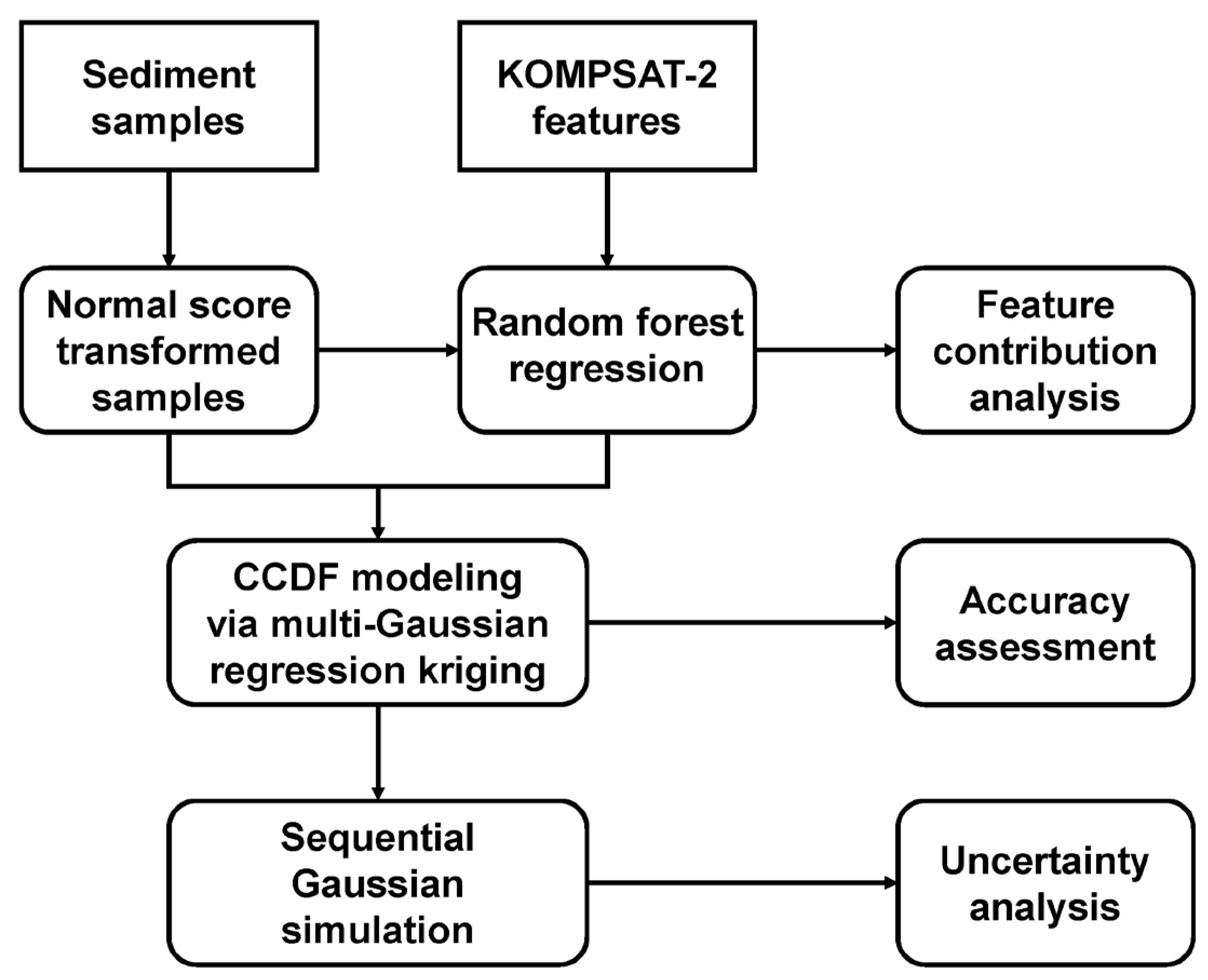
The workflow of the multivariate geostatistical simulation framework used herein is shown in Figure 4.
In this framework, the CCDF at all locations within the study area is first modeled using multivariate kriging. K2-derived features are incorporated into the CCDF modeling through multi-Gaussian regression kriging (MGRK) with RF regression. Based on the local CCDF models, sequential Gaussian simulation (SGS) is then performed to generate multiple alternative realizations of grain size at all locations. Summary statistics derived from these realizations are used to quantify prediction uncertainty.

2.3.1. CCDF Modeling

In geostatistics, uncertainty in grain size at any location is modeled using the CCDF, which provides the probability that the grain size is less than or equal to a given threshold. The CCDF can be constructed using either parametric multi-Gaussian kriging (MGK) or non-parametric indicator kriging [15]. As shown in Figure 2, the histogram of grain size values is not perfectly symmetric but does not exhibit strong skewness. When remote sensing-derived features are incorporated, indicator kriging becomes computationally intensive because it requires repeated variogram modeling and trend estimation for multiple threshold values. Considering these factors, MGK was selected in this study for CCDF modeling with K2-based features.
Suppose there are n observed sediment grain size samples, denoted as { z u α ; α = 1 , , n } , and M K2-derived features in the study area A, denoted as { z m u ; m = 1 , , M ,   u A } . Under the multi-Gaussian framework, the CCDF at any location u is assumed to follow a Gaussian distribution, with its mean and variance estimated through kriging [15]. To satisfy the Gaussian assumption, the sample data are first transformed using a normal score transform [30].
The CCDF at any location u ( F Y u ; y | ( I n f o . ) ) is modeled from the normal score transformed samples y u α ; α = 1 , , n   as follows:
F Y u ; y I n f o . = G [ y E [ Y ( u ) | I n f o . ] s t d [ Y ( u ) | I n f o . ] ]   ,
where G[ · ] is the standard Gaussian cumulative distribution function, and “|(Info.)” represents the conditional information (e.g., neighboring sample data). The normal score transformed grain size value is considered a realization of a random function Y u .   E [ Y ( u ) | I n f o . ] and s t d [ Y ( u ) | I n f o . ] are the mean and standard deviation, respectively, which define the Gaussian distribution. In univariate MGK, these correspond to the simple kriging estimate and the simple kriging standard deviation, respectively.

2.3.2. Multi-Gaussian Regression Kriging with Random Forest Regression

To incorporate K2-derived features into CCDF modeling, MGRK was employed in this study. In MGRK, the constant global mean in MGK is replaced with spatially varying local means (trend components of grain size), which are estimated using regression modeling with K2-derived features.
Given the trend component at any location u ( m * ( u ) ), the CCDF mean and standard deviation values are estimated as the MGRK estimate ( y * u ) and kriging standard deviation ( σ * u ):
y * u = α = 1 n ( u ) λ α ( u ) y u α m * u α + m * ( u ) ,
σ * u = 1 α = 1 n ( u ) λ α ( u ) C R u α u
where n ( u ) is the number of conditioning sample data within a search window centered on the estimation grid node u. λ α ( u ) and C R u α u   represent the simple kriging weights and the covariance function of the residuals between u α and u, respectively.
Before estimating the trend component from K2-derived features, the reflectance values of the blue, green, red, and NIR bands, along with NDWI, were found to be highly correlated, raising concerns about multicollinearity in regression modeling. To address this, LASSO regression [31] was first applied as a variable selection method to reduce redundancy and identify the most informative predictors. Using 5-fold cross-validation to determine the optimal penalty parameter, LASSO selected three variables, including green, red, and NDWI, with non-zero coefficients. However, the resulting linear model exhibited relatively low explanatory power (R2 = 21.7%), indicating that these features explained only a limited proportion of the variability in sediment grain size.
Given the limited explanatory power of the linear model, RF was adopted using the three LASSO-selected features to better capture nonlinear relationships and improve prediction accuracy. RF is an ensemble learning method that builds multiple decision trees for regression and classification [21]. In this study, in addition to the inherent feature importance measures provided by the RF model, SHAP [32], which can be readily integrated with RF predictions, was used to provide a more detailed and interpretable assessment of each feature’s contribution to the prediction. The number of trees in the RF model was determined through 5-fold cross-validation, ensuring robust predictive performance. For the SHAP analysis, the contribution of predictors was quantified using mean absolute SHAP values.

2.3.3. Sequential Gaussian Simulation

Once the CCDF at each grid node was modeled using MGRK, stochastic simulation was used to generate multiple equally probable realizations of grain size for uncertainty assessment. Each realization honors the sample data and reproduces sample statistics while avoiding the smoothing effects of kriging [23]. Since this study adopted a multi-Gaussian framework for CCDF modeling, SGS was used to generate the realizations. The SGS algorithm sequentially samples from the Gaussian CCDF modeled by MGRK and generates multiple realizations through back-transformation to the original data space [15].
The set of multiple values at each grid node can be interpreted as an approximation of a probability distribution function. In this study, the number of realizations was empirically set to 100. Preliminary tests demonstrated that changes in the number of realizations had little effect on the variability of the uncertainty measures, and the chosen value reflects a balance with computational efficiency. Various summary statistics can then be derived from this distribution, as described in the following subsection.

2.4. Evaluation

The effectiveness of incorporating K2-derived features into grain size mapping was evaluated both quantitatively and qualitatively using statistical indices and the spatial patterns of prediction results. Since the quality of geostatistical simulation depends largely on the accuracy of CCDF modeling, we first compared the predictive performance of univariate MGK and multivariate MGRK in modeling the CCDF. Leave-one-out cross-validation (LOOCV) was used to assess prediction accuracy. The back-transformed predictions were compared with the corresponding observed values excluded during the LOOCV process, and the mean absolute error (MAE) was computed as the error metric:
M A E = 1 n α = 1 n | z * u α z u α |   ,
where z * u α   is the estimated grain size obtained from either MGK or MGRK, depending on the method applied. Lower MAE values indicate better predictive performance
The mean squared deviation ratio (MSDR) [33] was also calculated to evaluate the consistency between predicted variances and actual prediction errors:
M S D R = 1 n α = 1 n ( z * u α z u α ) 2 σ 2 u α   ,
where σ 2 u α   is the variance estimated from the CCDF model. An MSDR value close to 1 suggests consistent uncertainty estimation.
The contribution of K2-derived features to grain size prediction was further evaluated by comparing spatial patterns and quantifying prediction uncertainty at unsampled locations. From the set of multiple realizations of grain size, the E-type estimate or mean and standard deviation were computed to summarize multiple simulation results and quantify prediction uncertainty, respectively.

2.5. Implementation

ENVI software version 6.1 (L3Harris Geospatial, Broomfield, CO, USA) was used for K2 image processing. All geostatistical analyses were conducted with GSLIB [30] and Isatis.neo version 2025.1 (Geovariances, Avon, France). Other procedures were implemented in the Python programming environment (version 3.12.3). The RF model was implemented using the scikit-learn library (version 1.4.2) [34], and SHAP values were computed using the SHAP library (version 0.45.1) [35].

3. Results

3.1. RF Regression Modeling Results

The trend components of the normal score transformed grain size values were estimated using RF regression modeling with three K2-derived features. The RF model, optimized via 5-fold cross-validation, achieved an R2 of 42.74%, indicating that the three K2 features explained 42.74% of the observed variability in the normal score transformed grain size. The remaining 57.26% of the variability was not explained by these features. To achieve a more complete representation of grain size variability, it is essential to address this residual component, which will be further modeled in the subsequent RK.
The variable importance ranking derived from the RF model showed that NDWI was the most influential predictor of grain size (0.408), followed by the red (0.317) and green (0.275) bands. Figure 5 presents the SHAP analysis results. The global summary plot (Figure 5a) confirms that NDWI has the strongest influence on the model output, as evidenced by its wide range of SHAP values. The dependence plot for NDWI, colored by red band reflectance (Figure 5b), reveals a nonlinear relationship: NDWI values above approximately 0.06 sharply increased SHAP values, indicating a strong positive effect on the predicted grain size. This effect is more pronounced when red band reflectance values are low, suggesting a possible interaction between the two variables.
The RF model developed at sample locations was then applied to all 4 m grids across the study area. Figure 6 illustrates the spatial distribution of the estimated trend component in Gaussian space, where the overlaid 94 sample locations allow comparison between the model trend and the field data. When comparing the estimated trend component with the sample values, a discrepancy was observed in the embayment area. High trend values were mainly observed in the southern intertidal zone, except for the bay area near Otjeom Port, in the eastern part of the study area. In contrast, most areas to the west and north of Seomot Island exhibited relatively low trend values. Halophyte communities located north and west of Halmi Island, as well as the surrounding areas of Seomot Island, showed trends values below 1. Higher trend values appeared mainly in the southern intertidal zone of Ojeomhange Bay, where a sand bank reduces wave and tidal energy, creating a low-energy environment. In contrast, Seomot Island’s western side, exposed to waves, showed lower values due to active sediment remobilization, while the northern tidal channel, sheltered from waves, also exhibited low trend values.

3.2. Geostatistical Modeling Results

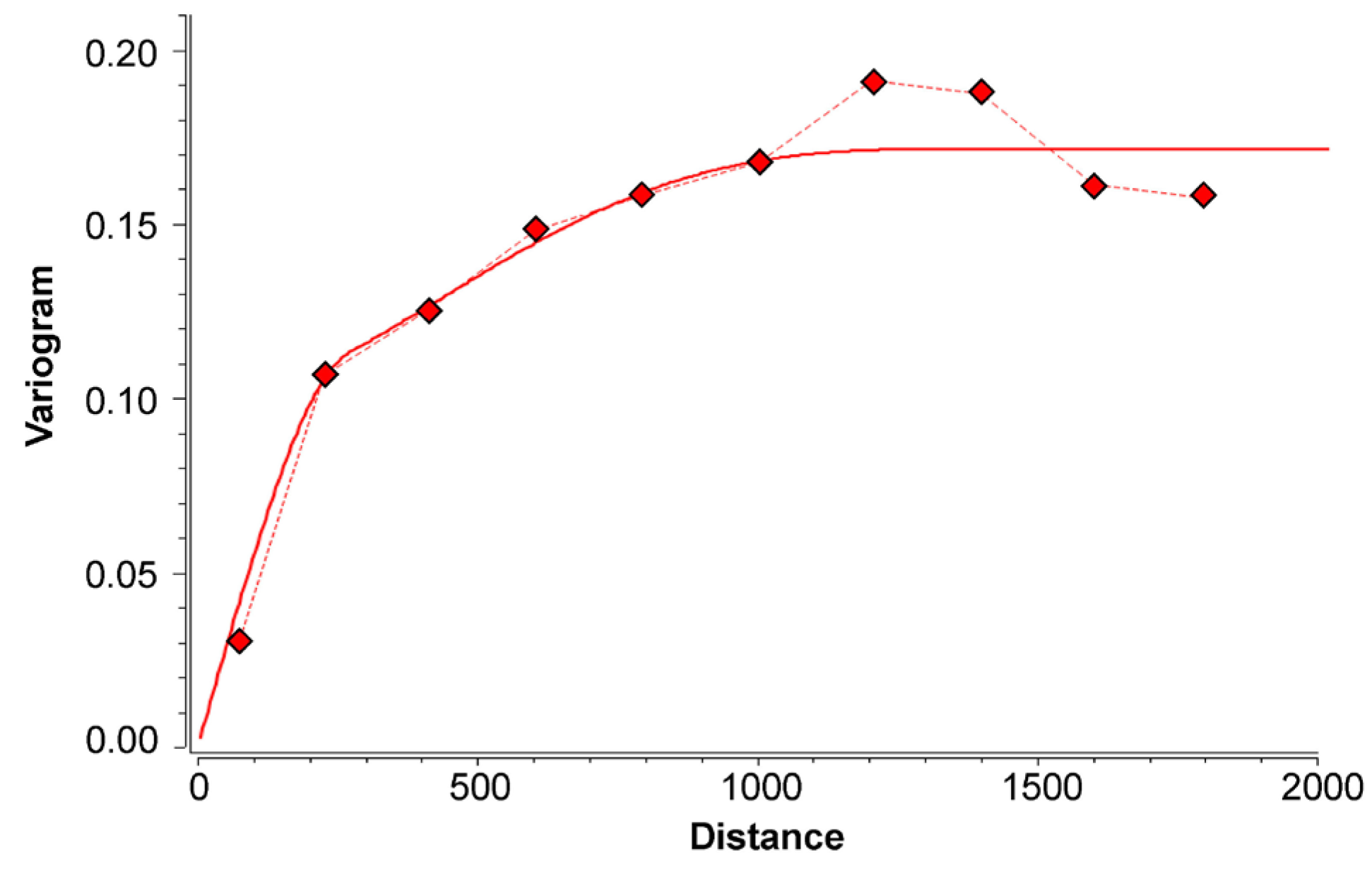
MGRK requires a variogram model for the residuals, rather than for the normal score transformed grain size. Figure 7 presents the experimental variograms and fitted models of the residuals. Since approximately 42.74% of the grain size variability was explained by the trend component, the sill of the residual variogram was substantially reduced to 0.17. The experimental variogram of the residuals did not exhibit distinct anisotropic spatial patterns. Therefore, isotropic variogram modeling was applied in this study. A nested isotropic variogram model was fitted using a spherical model with a range of 273 m and a cubic model with a range of 1450 m. The residual variogram exhibited a negligible nugget effect and spatial autocorrelation extending up to 1450 m, indicating that a clear spatial structure remained after removing the trend component. This result suggests that kriging of the residuals can meaningfully contribute to explaining the spatial variability of grain size. The residual variogram model shown in Figure 7 was used to estimate the CCDF mean and standard deviation.
Normal score back-transformed grain size predictions are shown in Figure 8. For comparison, MGK estimates based solely on field survey data are also shown. In both prediction results, fine sediments are predominantly distributed in the open sea area south of Otjeom Port, while coarse sediments are dominant around the tidal channels near Seomot Island. This distribution reflects coastal processes: the southern offshore area is sheltered by a sand bank that reduces hydrodynamic forcing and favors redeposition of suspended fine particles, while stronger tidal currents near the main channel enhance shear stress, leading to selective transport and the persistence of coarse-grained sediments. However, distinct differences exist between the two models. The MGK prediction shows a strong smoothing effect, which limits its ability to capture detailed spatial variations and makes it more suitable for identifying only general trends in grain size. In contrast, the MGRK prediction shows a more detailed depiction of grain size distribution across micro-landforms. Consistent with the trend component in Figure 6, fine sediments are generally found in areas with high trend values, whereas coarse sediments are more common in areas with low trend values. Nevertheless, the influence of the kriged residuals is evident, resulting in final predictions that reflect both the trend and residual components.
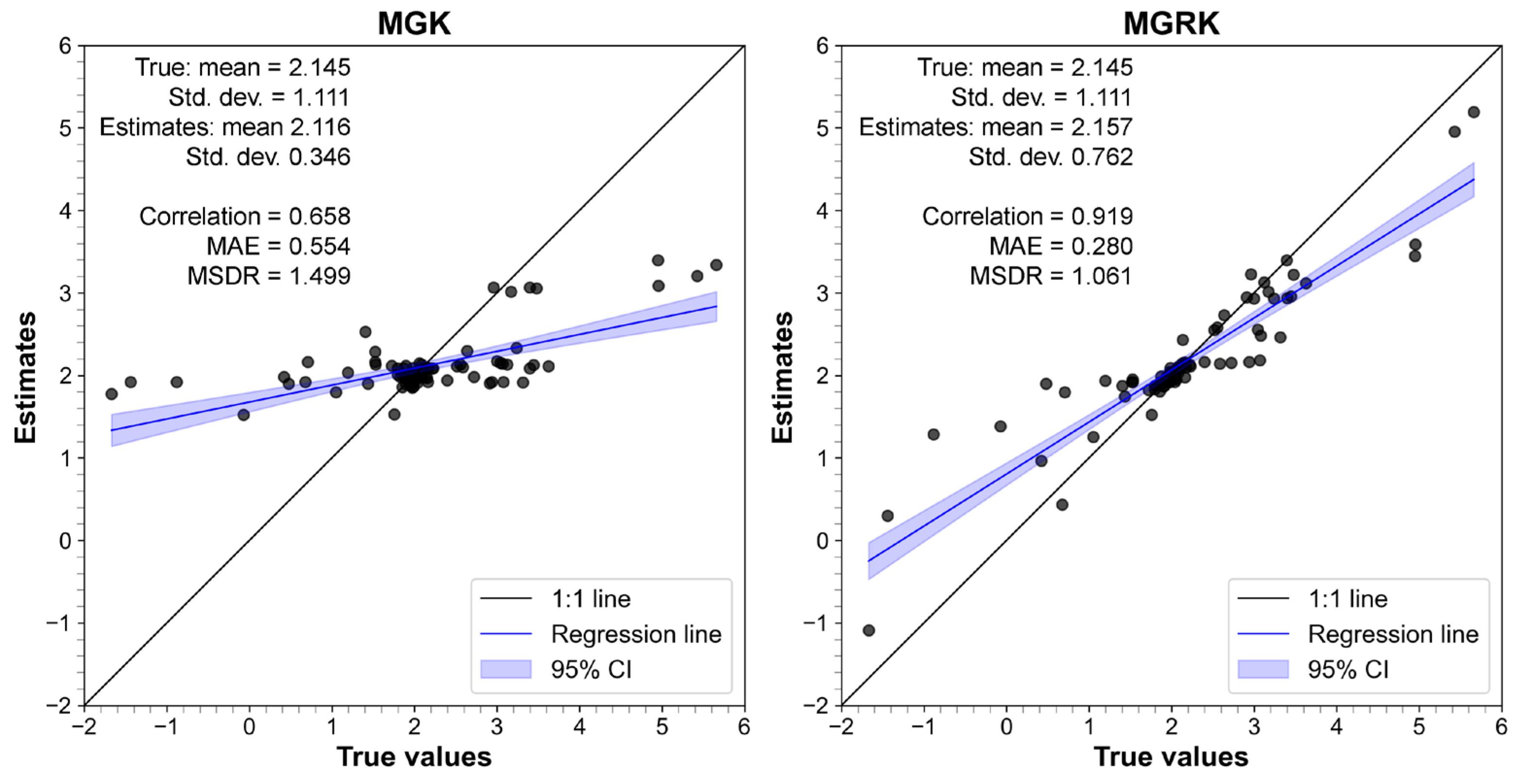
Figure 9 shows scatterplots of the true grain size values versus the LOOCV-based estimates for 94 samples. For comparison purposes, the MAE of regression-based predictions was also calculated. The MAEs of LASSO and RF were 0.804 and 0.653, respectively, both of which indicated larger errors than those of kriging-based predictions. In the comparison of kriging-based predictions, MGRK outperformed MGK in predictive performance. MGRK showed higher agreement with the true values compared to MGK. The MAE was substantially reduced from 0.554 in MGK to 0.280 in MGRK, corresponding to a relative improvement of approximately 49.5%. Both models tended to overestimate low values and underestimate high values, but this bias was more pronounced in MGK. As expected from Figure 8a, the standard deviation of MGK estimates (0.346) was much lower than that of the true values (1.111), indicating excessive smoothing. By comparison, MGRK produced a standard deviation of 0.762, providing a more realistic representation of grain size variability. The lower MSDR for MGRK suggests that MGRK provided a more reliable quantification of prediction uncertainty, whereas MGK underestimated uncertainty.

3.3. Simulation Results

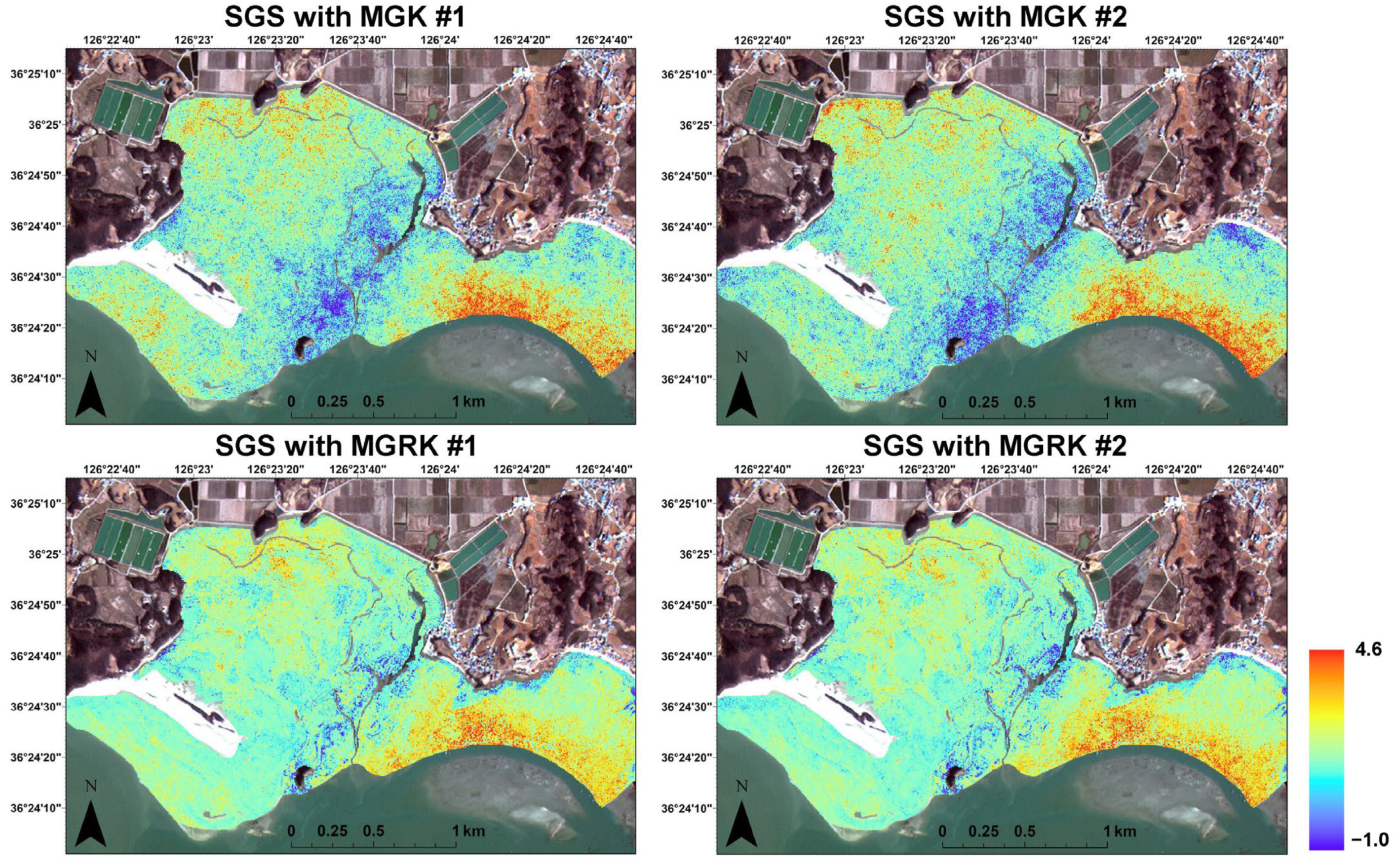
In this study, 100 realizations of sediment grain size were generated using SGS with both MGK and MGRK. Figure 10 presents the first two realizations generated from SGS with both MGK and MGRK. Individual realizations, which preserve sample values while reproducing spatial variability, illustrate the inherent variability of simulations, providing a basis for uncertainty assessment.
Figure 11 shows the mean of these 100 realizations. Compared to the kriging results in Figure 8, the mean of the simulations exhibits similar overall spatial patterns but displays greater spatial variability in grain size.
Prediction uncertainty, represented by the standard deviation at each pixel, is shown in Figure 12. The MGK-based simulation exhibits relatively high uncertainty across much of the study area (Figure 12a). In contrast, the SGS with MGRK shows a notable reduction in uncertainty over most regions, indicating that incorporating remote sensing-derived features leads to more consistent spatial predictions (Figure 12b). The mean standard deviation across the study area was 0.743 for the SGS with MGK and substantially lower at 0.280 for the SGS with MGRK. High uncertainty in the MGK-based simulation is mainly observed around Seomot Island, particularly near the northern tidal channels and in the offshore intertidal zone at the southeastern edge of Otjeom Port. Some degree of uncertainty is also found in the inner bay area. The cause of high uncertainty in MGK is the lack of field sampling data. Specifically, the offshore area south of Otjeom Port and the eastern part around Seomot Island consist of fine-grained sediments smaller than 4 phi, making field access difficult even at low tide and thus limiting sampling. In particular, in the eastern part of Seomot Island, high uncertainty is observed because the area is composed of fine-grained sediments, but most nearby sampling sites are located in tidal channels dominated by coarse sediments. These high-uncertainty regions show a marked reduction in the MGRK-based simulation, particularly around Seomot Island and in the tidal flats near the offshore area of Otjeom Port. However, elevated uncertainty remains in some of these areas.
A comparison between the mean of the realizations and the uncertainty distribution shows that areas with a high proportion of gravel and clay tend to exhibit greater uncertainty, whereas areas dominated by sand and silt show relatively lower uncertainty. Around the tidal channels near Seomot Island, the model predicted low grain size values (i.e., gravel), likely due to high flow velocity favoring gravel deposition. However, this area consists of a mixture of gravel and clay, and the elevated uncertainty is likely related to the limited number of samples near Seomot Island (i.e., fewer than three samples available within a 0.25 km2 unit area). In offshore clay-rich regions, the high moisture content associated with the open sea may not have been fully captured by K2-derived features. Furthermore, the influence of nearby sand and silt samples surrounding the clay samples may have contributed to the increased uncertainty in these areas.

4. Discussion

4.1. Contribution of the Study

Most previous studies on grain size mapping of intertidal surface sediments have attempted to improve accuracy by incorporating various remote sensing-derived auxiliary features, such as those from aerial imagery [5], SAR imagery [6], combined optical and SAR imagery [7], or UAV imagery [8], into regression models or multivariate kriging. However, these studies mainly focused on improving predictive performance and did not extend to addressing the uncertainty of predictions, which is the primary focus of this study.
The RF model applied in this study was useful for capturing nonlinear relationships between K2-derived features and grain size. The enhancement in accuracy and uncertainty reduction has direct practical implications for coastal management. For example, reducing MAE from 0.554 phi to 0.280 phi helps clarify the critical transition zone around the sand-mud boundary at 4 phi, where finer sediments are generally more erodible, where previous uncertainty could obscure erosion-prone areas. By providing more reliable maps, our approach enables managers to identify high-risk areas with greater confidence and allocate resources more effectively.
It is important to note, however, that the benefit of MGRK over MGK does not result solely from the incorporation of remote sensing-derived features using RF. Instead, it arises from combining the trend component estimated from these features with kriged residuals, which together improve modeling performance. The explanatory power of RF, reflected by an R2 of 42.74%, cannot be regarded as particularly high. Furthermore, the cross-validation R2 (31.99%) was lower than that obtained using all samples (42.74%). This result can be attributed to the limited sample size (n = 94) and the restricted set of input features, indicating that the generalization performance of the standalone RF model may be insufficient. Nevertheless, the proposed MGRK approach compensates for this limitation by incorporating residual correction. Considering the practical difficulty of collecting extensive field samples in tidal flats, the proposed method, which combines trends derived from satellite imagery with kriged residuals, demonstrates both practical applicability and methodological contribution.
Rather than focusing solely on spatial prediction, this study employed a simulation-based approach to quantify prediction uncertainty at unsampled locations. The reduction in uncertainty observed in the MGRK-based simulations, which incorporated remote sensing-derived features, suggests that this approach not only improves prediction accuracy but also enhances the reliability of predictions. Additionally, uncertainty maps can guide the prioritization of future field survey locations. For example, in the vicinity of Seomot Island, elevated uncertainty was observed, likely due to the relatively sparse sampling density and the heterogeneous sedimentary environment (e.g., clay-gravel mixture zone). This highlights how the uncertainty map can identify data gaps and indicate where targeted sampling would be most beneficial.
The CCDF modeled by kriging (e.g., MGK or MGRK) already provides pixel-based local uncertainty. Quantitative measures of the CCDF spread can be used to assess prediction uncertainty [15]. For example, the standard deviation of the CCDF should be similar to that derived from multiple realizations in a simulation approach as the number of simulations increases. However, unlike the kriging-based local uncertainty modeling, simulation offers additional advantages for uncertainty quantification, particularly when a change of support or joint-pixel analysis is required. The CCDF model constructed at a 4 m resolution in the kriging framework cannot be directly transferred to coarser scales or used for joint uncertainty modeling, such as when integrating with coarse-scale environmental variables or assessing uncertainty across multiple pixels. In contrast, simulation overcomes these limitations. Individual realizations, which retain more spatial variability, can be easily aggregated to coarser resolutions and used for multiple pixel or zonal analysis. By calculating proportions across multiple realizations, the probability of exceeding specific thresholds or belonging to particular sediment classes can be easily estimated. Therefore, simulation-based spatial uncertainty modeling offers potential advantages for coastal management, as it can be applied to predicting tidal flat morphology evolution, assessing erosion risk along sand-mud boundaries, and supporting decision-making for vulnerable coasts at broader spatial scales.
Another key advantage of the simulation approach for grain size mapping is its ability to evaluate the impact of grain size maps on model outputs. For instance, using different realizations of grain size as input for surface sediment classification or habitat suitability modeling [36,37] enables probabilistic interpretations of model outputs. For example, sediment grain size distribution is a key determinant of benthic species habitats, as many benthic organisms are strongly associated with particular sediment types. By employing multiple realizations of grain size, probabilistic habitat suitability maps for benthic species can be generated, which explicitly account for uncertainty. This probabilistic perspective provides more reliable decision-supporting information for conservation planning, fishery management, and coastal spatial planning.

4.2. Limitations and Future Research Directions

Surface moisture is known to be associated with sediment grain size [1]. Given the restricted four-band configuration of high-spatial resolution satellite imagery, such as KOMPSAT-2, NDWI represents the most appropriate spectral index available for capturing tidal flat moisture conditions. However, as the present results rely on imagery from a single acquisition date, additional validation with datasets obtained at different times or seasons will be necessary. In addition to more extensive experiments using imagery acquired under diverse temporal and environmental conditions, incorporating additional moisture-related features, such as tidal channel density derived from high-resolution optical imagery [20], may further enhance predictive performance. Likewise, backscattering coefficients from high-resolution SAR imagery, which are sensitive to both moisture content and surface roughness [12], could also be valuable auxiliary features for characterizing tidal flat sedimentary environments.
From the perspective of data supplementation, the prediction uncertainty observed in this study appears to arise not only from the limited sample availability but also from fine-scale sediment heterogeneity that remains unresolved at the spatial resolution of K2 imagery. To reduce such uncertainty, particularly in environments where collecting sufficient field samples is challenging, the use of fine-scale auxiliary data becomes essential. UAV imagery, with its centimeter-level resolution, can capture subtle sedimentary heterogeneity that is not captured by satellite imagery, thereby complementing scarce field samples and helping to mitigate regional uncertainties. Future experiments incorporating UAV imagery as secondary information will be valuable for further improving predictive performance and reliability. Therefore, future studies should include additional experiments in both of these directions to more comprehensively evaluate the influence of input features on intertidal surface sediment grain size mapping.
Although tidal stage can influence tidal flat exposure and surface wetness, the impact was minimized in this study by using imagery acquired near the lowest low tide. Both tidal conditions and intrinsic sediment properties can affect surface reflectance and moisture indices. A limitation of this study, however, is the reliance on imagery from a single acquisition date. Future studies should therefore incorporate imagery collected under different tidal stages to more explicitly evaluate the combined effects of exposure time and sediment composition on spectral indices and prediction performance. In addition, given the site-specific nature of tidal flats, the broader applicability of the findings to other regions remains uncertain and requires validation through additional experiments in different tidal flat environments.
From a theoretical perspective, the integration of remote sensing-derived features with field survey data is based on decomposing grain size into a deterministic trend component and a stochastic residual component. Remote sensing-derived features are used to estimate the deterministic trend component, but the uncertainty of this estimation is not explicitly modeled. As a result, uncertainty modeling in simulation is subject to the stochastic residual component, and the contribution of remote sensing-derived features is inferred only through improvements in explanatory power and predictive performance. This presents a limitation in fully understanding the role of individual features. Bayesian hierarchical spatial models [38] and the INLA-SPDE approach [39] allow simultaneous estimation of both trend and residual components while explicitly modeling their associated uncertainties. These methods provide probabilistic estimates of the trend component and can incorporate its uncertainty into the overall prediction process. In addition to INLA, general-purpose probabilistic programming frameworks such as PyMC [40] and Stan [41] can also be employed to implement Bayesian hierarchical models. These tools provide flexibility in modeling complex environmental processes that may exhibit non-stationarity and allow prior knowledge or physical constraints to be incorporated directly into the model. If the uncertainty associated with the trend component estimation could be quantified, it would enable a more comprehensive assessment of feature contributions and the benefits of incorporating additional features. Future research should explore these approaches to improve spatial prediction and uncertainty quantification in thematic mapping that integrates remote sensing-derived features and field survey data in tidal flats.

5. Conclusions

This study proposed a hybrid geostatistical simulation approach that integrates remote sensing-derived features with sparse field survey data to improve the accuracy of grain size prediction and quantify prediction uncertainty. An experiment using field measurements and features derived from high-resolution K2 imagery in the Baramarae tidal flat in Korea demonstrated the effectiveness of the proposed approach. The proposed approach achieved higher prediction accuracy and reduced uncertainty compared to the conventional approach based solely on sparse field survey data. Specifically, the simulation-based approach with K2-derived features achieved the lowest error (MAE = 0.280), compared with 0.554 for field survey data alone and 0.653 for RF regression modeling, clearly demonstrating the advantage of combining regression models with geostatistical methods.
Future applications of grain size simulations for broader coastal applications, such as shoreline change monitoring, sediment transport studies, and climate-driven coastal management, would enhance the practical relevance of the presented approach. With methodological improvements, such as quantifying the uncertainty of trend components, and the design of extensive experiments under diverse conditions, the presented approach could provide valuable decision-supporting information in the context of coastal management.

Author Contributions

Conceptualization, N.-W.P. and D.-H.J.; methodology, N.-W.P.; validation, N.-W.P.; formal analysis, N.-W.P.; investigation, N.-W.P. and D.-H.J.; data curation, D.-H.J.; writing—original draft preparation, N.-W.P. and D.-H.J.; writing—review and editing, N.-W.P. All authors have read and agreed to the published version of the manuscript.

Funding

This work was supported by the Inha University Research Grant.

Data Availability Statement

Only field survey data supporting the conclusions of this article will be made available by the authors on request. The high-resolution satellite imagery used in this study was obtained under a commercial license and cannot be shared.

Conflicts of Interest

The authors declare no conflicts of interest.

References

  1. Ryu, J.-H.; Choi, J.-K.; Lee, Y.-K. Potential of remote sensing in management of tidal flats: A case study of thematic mapping in the Korean tidal flats. Ocean Coast. Manag. 2014, 102, 458–470. [Google Scholar] [CrossRef]
  2. Schrijvershof, R.A.; Van Maren, D.S.; Van der Wegen, M.; Hoitink, A.J.F. Land reclamation controls on multi-centennial estuarine morphodynamics. Earth’s Future 2024, 12, e2024EF005080. [Google Scholar] [CrossRef]
  3. Cox, J.R.; Lingbeek, J.; Weisscher, S.A.; Kleinhans, M.G. Effects of sea-level rise on dredging and dredged estuary morphology. J. Geophys. Res. Earth Surf. 2022, 127, e2022JF006790. [Google Scholar] [CrossRef]
  4. Zhang, R.; Zhou, H.; Gao, S.; Wang, Y.; Xu, W. Impacts of tidal flat reclamation on suspended sediment dynamics in the tidal-dominated Wenzhou Coast, China. Front. Mar. Sci. 2023, 10, 1097177. [Google Scholar] [CrossRef]
  5. Rainey, M.P.; Tyler, A.N.; Givear, D.J.; Bryant, R.G.; McDonald, P. Mapping intertidal estuarine sediment grain size distributions through airborne remote sensing. Remote Sens. Environ. 2003, 86, 480–490. [Google Scholar] [CrossRef]
  6. Van Der Wal, D.; Herman, P.M.J.; Wielemaker-Van Den, D. Characterisation of surface roughness and sediment texture of intertidal flats using ERS SAR imagery. Remote Sens. Environ. 2005, 98, 96–109. [Google Scholar] [CrossRef]
  7. Van Der Wal, D.; Herman, P.M.J. Regression-based synergy of optical, shortwave infrared and microwave remote sensing for monitoring the grain-size of intertidal sediments. Remote Sens. Environ. 2007, 111, 89–106. [Google Scholar] [CrossRef]
  8. Kim, M.; Baek, W.-K.; Jung, H.S.; Ryu, J.-H. Analysis of micro-sedimentary structure characteristics using ultra-high resolution UAV imagery: Hwangdo tidal flat, South Korea. Korean J. Remote Sens. 2024, 40, 295–305, (In Korean with English Abstract). [Google Scholar]
  9. Yates, M.G.; Jones, A.R.; McGroty, S.; Goss-Custard, J.D. The use of satellite imagery to determine the distribution of intertidal surface sediments of The Wash, England. Estuar. Coast. Shelf Sci. 1993, 36, 333–344. [Google Scholar] [CrossRef]
  10. Kim, K.-L.; Kim, B.-J.; Lee, Y.-K.; Ryu, J.-H. Generation of a large-scale surface sediment classification map using unmanned aerial vehicle (UAV) data: A case study at the Hwang-do tidal flat, Korea. Remote Sens. 2019, 11, 229. [Google Scholar] [CrossRef]
  11. Kim, M.; Park, J.; Hyun, C.-U. Evaluating changes in blue carbon storage by analyzing tidal flat areas using multi-temporal satellite data in the Nakdong River estuary, South Korea. Korean J. Remote Sens. 2024, 40, 191–202, (In Korean with English Abstract). [Google Scholar]
  12. Park, N.-W. Geostatistical integration of field measurements and multi-sensor remote sensing images for spatial prediction of grain size of intertidal surface sediments. J. Coast. Res. 2019, 90, 190–196. [Google Scholar] [CrossRef]
  13. Klemas, V. Remote sensing techniques for studying coastal ecosystems: An overview. J. Coast. Res. 2011, 27, 2–17. [Google Scholar]
  14. Park, N.-W.; Jang, D.-H.; Chi, K.-H. Integration of IKONOS imagery for geostatistical mapping of sediment grain size at Baramarae beach, Korea. Int. J. Remote Sens. 2009, 30, 5703–5724. [Google Scholar] [CrossRef]
  15. Goovaerts, P. Geostatistics for Natural Resources Evaluation; Oxford University Press: New York, NY, USA, 1997. [Google Scholar]
  16. Hengl, T.; Heuyvelink, G.B.M.; Rossiter, D.G. About regression-kriging: From equations to case studies. Comput. Geosci. 2007, 33, 1301–1315. [Google Scholar] [CrossRef]
  17. Goovaerts, P. Geostatistical approaches for incorporating elevation into the spatial interpolation of rainfall. J. Hydrol. 2000, 228, 113–129. [Google Scholar] [CrossRef]
  18. Dobermann, A.; Ping, J.L. Geostatistical integration of yield monitor data and remote sensing improves yield maps. Agron. J. 2004, 9, 285–297. [Google Scholar] [CrossRef]
  19. Kerry, R.; Goovaerts, P.; Rawlins, B.G.; Marchant, B.P. Disaggregation of legacy soil data using area to point kriging for mapping soil organic carbon at the regional scale. Geoderma 2012, 170, 347–358. [Google Scholar] [CrossRef]
  20. Kwak, G.-H.; Kim, K.; Lee, J.; Ryu, J.-H. Unmanned aerial vehicles images based tidal flat surface sedimentary facies mapping using regression kriging. Korean J. Remote Sens. 2023, 39, 537–549, (In Korean with English Abstract). [Google Scholar]
  21. Breiman, L. Random forests. Mach. Learn. 2001, 45, 5–32. [Google Scholar] [CrossRef]
  22. Hutengs, C.; Vohland, M. Downscaling land surface temperatures at regional scales with random forest regression. Remote Sens. Environ. 2016, 178, 127–141. [Google Scholar] [CrossRef]
  23. Chilès, J.-P.; Delfiner, P. Geostatistics: Modeling Spatial Uncertainty, 2nd ed.; Wiley: Hoboken, NJ, USA, 2012. [Google Scholar]
  24. Jang, D.-H.; Kim, J.-S.; Park, N.-W. Characteristics variation of the sedimentary environment in winter season around the Baramarae Beach of Anmyeondo using surface sediment analysis. J. Korean Geomroph. Assoc. 2010, 17, 15–27, (In Korean with English Abstract). [Google Scholar]
  25. Khodada, S.; Jang, D.-H. Analysis of landform changes and sedimentary environment characteristics during winter season around the Baramarae Beach, Anmyeondo in Korea’s west coast. J. Korean Geomroph. Assoc. 2014, 21, 95–109, (In Korean with English Abstract). [Google Scholar]
  26. Kim, Y.; Jang, D.-H.; Park, N.-W.; Yoo, H.Y. Assessment of landform changes in Baramarae tidal flat, Korea using combined analysis of multi-temporal remote sensing images and grain size measurement data. J. Mar. Sci. Tech. 2016, 24, 1070–1080. [Google Scholar]
  27. Roberts, W.; Le Hir, P.; Whitehouse, R.J.S. Investigation using simple mathematical models of the effect of tidal currents and waves on the profile shape of intertidal mudflats. Cont. Shelf Res. 2000, 10–11, 1079–1097. [Google Scholar] [CrossRef]
  28. Park, N.-W.; Jang, D.-H. Geostatistical classification of intertidal surface sediments using log-ratio transformation and high-resolution remote sensing imagery. J. Coast. Res. 2020, 102, 157–165. [Google Scholar] [CrossRef]
  29. McFeeters, S.K. The use of the Normalized Difference Water Index (NDWI) in the delineation of open water features. Int. J. Remote Sens. 1996, 17, 1425–1432. [Google Scholar] [CrossRef]
  30. Deutsch, C.V.; Journel, A.G. GSLIB: Geostatistical Software Library and User’s Guide, 2nd ed.; Oxford University Press: New York, NY, USA, 1998. [Google Scholar]
  31. Tibshirani, R. Regression shrinkage and selection via the lasso. J. R. Stat. Soc. Ser. B Stat. Methodol. 1996, 58, 267–288. [Google Scholar] [CrossRef]
  32. Lundberg, S.M.; Lee, S.-I. A Unified Approach to Interpreting Model Predictions. In Proceedings of the 31st International Conference on Neural Information Processing Systems (NeurIPS), Long Beach, CA, USA, 4–9 December 2017; pp. 4768–4777. [Google Scholar]
  33. Oliver, M.A.; Webster, R. A tutorial guide to geostatistics: Computing and modelling variograms and kriging. Catena 2014, 113, 56–69. [Google Scholar] [CrossRef]
  34. Scikit-Learn: Machine Learning in Python. Available online: https://scikit-learn.org (accessed on 26 May 2025).
  35. SHAP Documentation. Available online: https://shap.readthedocs.io (accessed on 26 May 2025).
  36. Choi, J.-K.; Oh, H.-J.; Koom, B.J.; Lee, S.; Ryu, J.-H. Macrobenthos habitat mapping in a tidal flat using remotely sensed data and a GIS-based probabilistic model. Mar. Pollut. Bull. 2011, 62, 564–572. [Google Scholar] [CrossRef]
  37. Puls, W.; Van Bernem, K.-H.; Eppel, D.; Kapitza, H.; Pleskachevsky, A.; Riethmüller, R.; Vaessen, B. Prediction of benthic community structure from environmental variables in a soft-sediment tidal basin (North Sea). Helgol. Mar. Res. 2012, 66, 345–361. [Google Scholar] [CrossRef][Green Version]
  38. Banerjee, S.; Carlin, B.P.; Gelfand, A.E. Hierarchical Modeling and Analysis for Spatial Data; Chapman & Hall/CRC: Boca Raton, FL, USA, 2004. [Google Scholar][Green Version]
  39. Blangiardo, M.; Cameletti, M. Spatial and Spatio-Temporal Bayesian Models with R-INLA; Wiley: Chichester, UK, 2015. [Google Scholar][Green Version]
  40. PyMC. Available online: https://www.pymc.io/welcome.html (accessed on 9 September 2025).[Green Version]
  41. Stan: Software for Bayesian Data Analysis. Available online: https://mc-stan.org/ (accessed on 9 September 2025).[Green Version]
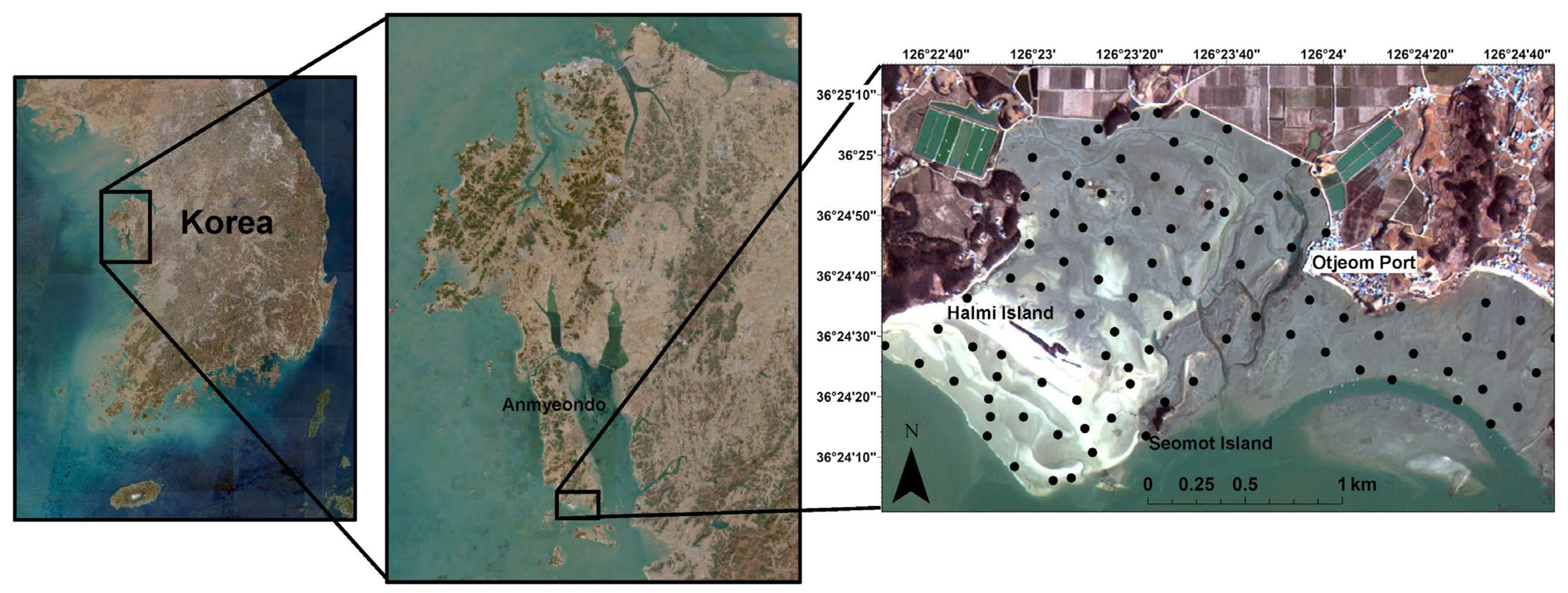
Figure 1. Location of the study area and distribution of field survey measurement points (black dots). The background is KOMPSAT-2 natural color imagery.
Remotesensing 17 03230 g001
Figure 2. Histogram of the mean grain size of 94 surface sediment samples with summary statistics.
Remotesensing 17 03230 g002
Figure 3. Selected features derived from KOMPSAT-2 imagery: (a) red band reflectance; (b) NDWI. The background is KOMPSAT-2 natural color imagery.
Remotesensing 17 03230 g003
Figure 4. Schematic overview of the geostatistical simulation framework integrating remote sensing-derived features and quantifying uncertainty for sediment grain size mapping.
Remotesensing 17 03230 g004
Figure 5. SHAP plots: (a) global summary plot; (b) dependence plot for NDWI, colored by red band reflectance.
Remotesensing 17 03230 g005
Figure 6. Trend components of grain size in Gaussian space estimated using RF. Sample locations are shown as circles, colored according to the same scale.
Remotesensing 17 03230 g006
Figure 7. Experimental variograms (dots with dashed lines) and fitted models (solid line) of residuals.
Remotesensing 17 03230 g007
Figure 8. Grain size estimation results: (a) MGK; (b) MGRK.
Remotesensing 17 03230 g008
Figure 9. Scatterplots of true grain size values and LOOCV-based estimates obtained from MGK and MGRK. Regression lines with 95% confidence intervals are shown, and summary and error statistics are included for performance evaluation.
Remotesensing 17 03230 g009
Figure 10. Sets of the first two realizations of SGS with MGK and SGS with MGRK.
Remotesensing 17 03230 g010
Figure 11. Mean of 100 realizations: (a) SGS with MGK; (b) SGS with MGRK.
Remotesensing 17 03230 g011
Figure 12. Standard deviation of 100 realizations: (a) SGS with MGK; (b) SGS with MGRK.
Remotesensing 17 03230 g012
Disclaimer/Publisher’s Note: The statements, opinions and data contained in all publications are solely those of the individual author(s) and contributor(s) and not of MDPI and/or the editor(s). MDPI and/or the editor(s) disclaim responsibility for any injury to people or property resulting from any ideas, methods, instructions or products referred to in the content.