Article

Stacking-Based Solar-Induced Chlorophyll Fluorescence Downscaling for Soil EC Estimation

1
College of Geography and Remote Sensing Sciences, Xinjiang University, Urumqi 830046, China
2
Xinjiang Institute of Technology, Aksu 843100, China
*
Author to whom correspondence should be addressed.
Remote Sens. 2025, 17(18), 3222; https://doi.org/10.3390/rs17183222
Submission received: 1 July 2025 / Revised: 29 August 2025 / Accepted: 13 September 2025 / Published: 18 September 2025

Abstract

Highlights

What are the main findings?
  • A Stacking model effectively downscales Solar-Induced Chlorophyll Fluorescence (SIF) from 0.05° to 30 m resolution with high accuracy.
  • Fusing the downscaled SIF with environmental covariates significantly improves soil electrical conductivity (EC) estimation.
What is the implication of the main finding?
  • High-resolution SIF acts as a sensitive proxy for soil salinity by capturing fine-scale vegetation stress missed by coarser data.
  • This study pioneers the novel use of SIF for soil EC estimation, demonstrating a previously underexplored remote sensing application for soil health monitoring.

Abstract

The Xinjiang Province of China, characterized as a typical arid to semi-arid region, is increasingly facing severe issues related to soil salinization. Timely and accurate estimation of soil salinization in this region is crucial for the sustainable development of agriculture and food security. However, current methods for detecting soil salinization primarily rely on various environmental covariates, which assess the extent of soil salinization by analyzing the relationship between environmental factors and the accumulation of soil salts. Nonetheless, these conventional environmental covariates often suffer from response delays, making it challenging to promptly reflect the dynamic changes in soil salinity. Solar-induced chlorophyll fluorescence (SIF) has been widely used to assess vegetation photosynthetic efficiency and is considered a direct indicator of plant photosynthetic activity. In contrast, SIF provides a timely means of monitoring the status of plant photosynthesis, indirectly reflecting the impact of soil salinization on plant growth. However, the spatial resolution of SIF products derived from satellites is typically low, which significantly limits the accurate estimation of soil salinization in Xinjiang. This study proposes a novel method for monitoring soil salinization, based on SIF data. The approach employs a Stacking ensemble learning model to downscale SIF data, thereby improving the spatial resolution of soil salinity monitoring. Using the GOSIF dataset, combined with environmental covariates, such as MODIS, the Stacking framework facilitates the fine-scale downscaling of SIF data, generating high-resolution SIF products, ranging from 0.05° to 0.005°, with a spatial resolution of 30 m. This refined SIF data is then used to predict soil electrical conductivity (EC). The experimental results demonstrate that: (1) the proposed Stacking-based SIF downscaling method is highly effective, with a high degree of fit to reference SIF data (R2 > 0.85); (2) the high-resolution SIF data, after downscaling, more accurately reflects the spatial heterogeneity of soil salinization, especially in shallow soils (r < −0.6); and (3) models combining SIF and environmental covariates exhibit superior accuracy compared to models that rely solely on SIF or traditional environmental covariates (R2 > 0.65). This research provides new data support and methodological advancements for precision agriculture and ecological environmental monitoring.

1. Introduction

Xinjiang, a typical arid to semi-arid region in China, is increasingly facing severe soil salinization problems. Due to factors such as intense evaporation, improper irrigation, and poor drainage, soil salts continue to accumulate in the surface layers, leading to widespread degradation of farmland quality. The most severe salinization occurs in areas such as the lower reaches of the Tarim River, around Aibi Lake, and in some of the older irrigation districts [1]. This phenomenon not only leads to the destruction of soil structure, stunted crop growth, and a decline in agricultural yields, but also triggers a series of ecological and environmental issues, such as vegetation degradation, reduced biodiversity, and groundwater pollution. Consequently, it poses a significant threat to regional ecological security and the sustainable development of agriculture [2].
The Aksu region of Xinjiang, a key agricultural area in southern Xinjiang, is facing a critical soil salinization issue, which has become a major limiting factor for the sustainable development of local agriculture [3]. Influenced by the arid climate of the Taklamakan Desert, the region experiences an average annual evaporation rate that far exceeds precipitation. Additionally, the long-term use of traditional flood irrigation in the Tarim River irrigation district has led to rising groundwater levels, causing a significant accumulation of salts at the soil surface through capillary action. Soil salinization is particularly pronounced around the city of Aksu, the central part of Wensu County, and the northern part of Awati County. Scientific studies have reported a regional average topsoil electrical conductivity (EC) as high as 18.3 dS/m, which classifies the area as severely salinized. Consequently, large areas often exceed the moderately saline threshold of 8 dS/m and, in the most affected zones, EC values climb well above 16 dS/m, exceeding the tolerance limit of most crops and resulting in farmland abandonment. This situation not only results in soil hardening, decreased fertility, and reduced crop yields [4], but has further triggered a series of chain reactions: on one hand, it has increased the economic burden on farmers, and, on the other hand, it has exacerbated regional ecological degradation, particularly intensifying the ecological and environmental conflicts related to ecological water transfers in the lower reaches of the Tarim River [5]. The negative impacts of soil salinization on the local ecosystem, such as vegetation degradation and reduced biodiversity, have also attracted widespread attention.
Currently, methods for detecting soil salinization primarily rely on various environmental covariates, which exhibit distinct spatial and temporal responses to salt dynamics. For instance, climatic conditions such as the balance between precipitation and evapotranspiration govern long-term salt accumulation trends; arid and semi-arid regions with high evaporation rates often experience upward capillary movement of saline groundwater, leading to surface salinization, particularly during dry seasons. Hydrological characteristics, especially the groundwater depth, are critical at a local scale. In low-lying areas or areas with shallow water tables, salt is more readily transported to the root zone and soil surface. Remote sensing indicators like the Normalized Difference Vegetation Index (NDVI) and the Enhanced Vegetation Index (EVI) are widely used for large-scale monitoring. These indices assess salinization indirectly by quantifying vegetation health, based on the principle that high soil salinity induces plant stress and reduces canopy vigor, resulting in lower index values. However, the applicability of these vegetation indices is temporally constrained by the growing season, and they can be confounded by other stressors like drought or disease. Furthermore, they are less effective in sparsely vegetated areas or at the early stages of salinization, before vegetation is visibly affected. Therefore, these methods assess the extent of soil salinization by analyzing the complex, scale-dependent relationships between these environmental factors and soil salt accumulation [6]. However, these environmental covariates often suffer from response delays, making it difficult to promptly reflect the dynamic changes in soil salinity [7]. SIF has been widely used to assess vegetation photosynthetic efficiency [8]. The basis of this method is that plants absorb light energy during photosynthesis and re-emit a portion of it as fluorescence. This fluorescence signal is primarily concentrated in the 680–750 nm (red light) and 750–800 nm (near-infrared) wavelength bands, and is considered a direct indicator of plant photosynthetic efficiency [9]. In contrast, SIF can provide timely monitoring of plant photosynthetic activity and indirectly reflect the impact of soil salinization on plant growth. Thus, SIF is emerging as a promising tool for studying soil salinization. By providing a timely measure of plant photosynthetic activity, SIF can indirectly reflect plant stress caused by soil salinity [10].
However, due to the limitations of satellite technology, existing satellite-derived SIF products struggle to achieve high temporal and spatial resolution. These SIF data remain relatively coarse in regard to many research areas, such as regional carbon cycle studies, crop growth research, and drought detection [11]. Moreover, in agricultural areas of China, farmland is fragmented. These lower-resolution SIF products are not accurate enough for regional agricultural drought monitoring. Therefore, to obtain high-resolution SIF products, various downscaling methods have been proposed. For example, Gensheimer used convolutional neural networks to downscale SIF data, generating higher resolution SIF data to improve its application in agriculture, ecological monitoring, and crop growth analysis [12]. Tao, on the other hand, generated a high-resolution SIF dataset for China, from 2000 to 2022, using TROPOMI [13]. Kang et al. employed downscaling methods to reduce OCO-2 SIF data to a resolution of 0.008° for detecting agricultural drought in Henan, China [10]. The new SIF was subsequently used to monitor the corn growing season in Henan Province. These studies demonstrate that downscaling methods not only enhance the spatial resolution of SIF data, but also provide more accurate observational data for fields such as agriculture and drought monitoring.
To address the issue of low spatial resolution in existing satellite-derived SIF products, this study aims to downscale SIF data. A primary objective is to apply this high-resolution SIF data to soil salinization monitoring. The key connection is as follows: soil salinization is a major stressor that limits agricultural productivity by inhibiting plant physiological functions and, consequently, photosynthesis. As a direct signal from the photosynthetic process, SIF can effectively indicate this vegetation stress. However, soil salinization often occurs in patches, exhibiting strong spatial heterogeneity that cannot be effectively identified by coarse-resolution native SIF products. To overcome this limitation, this study proposes the use of a Stacking framework. As an ensemble learning method, Stacking improves the model’s predictive accuracy and robustness by combining the predictions of multiple base learners [14]. Moreover, the Stacking framework offers significant advantages in terms of handling complex nonlinear relationships and integrating multi-source data, enabling it to more accurately capture the spatial heterogeneity caused by soil salinization [15].
To this end, this study aims to achieve fine-scale detection of soil salinity in the Aksu region of Xinjiang, using the raw SIF dataset. The specific objectives include: (1) progressively downscaling the GOSIF dataset from 0.05° to a 30 m resolution, developing a high-precision Stacking–SIF downscaling prediction model, suitable for the Aksu region, and validating its accuracy and application potential; (2) developing an SIF–EC model based on the downscaled SIF data to accurately predict soil EC in the Aksu region; and (3) generating spatial distribution maps of soil EC at different depths in the Aksu region by integrating multi-source remote sensing data and ground-based sample measurements, enabling the precise detection of soil salinity in the Aksu area.

2. Materials and Methods

2.1. Study Area

The study area is situated in the Aksu region, a representative oasis agricultural zone, located in the western part of the Xinjiang Uygur Autonomous Region. Geographically, it occupies a critical transitional zone at the southern foot of the central Tianshan Mountains and the northwestern margin of the Tarim Basin, with coordinates ranging from 75°35′ to 80°59′ E and 40°17′ to 42°27′ N, as shown in Figure 1. The topography is dominated by the piedmont alluvial plain of the Aksu River, an upper tributary of the Tarim River, with an altitude generally ranging from 950 to 1200 m. This region is characterized by a temperate continental arid climate, marked by significant thermal contrasts. It experiences long, hot, and dry summers and cold winters, with a large diurnal and annual temperature range. The average annual temperature is approximately 10–12 °C. The climatic conditions are defined by scarce precipitation and intense potential evapotranspiration. The average annual precipitation is merely 50–80 mm, while the average annual potential evaporation can exceed 2300 mm. This extreme imbalance between evaporation and precipitation is a primary driver of upward salt migration in the soil profile. Hydrologically, the region’s agriculture is almost entirely dependent on irrigation from the Aksu and Tarim Rivers, which are fed by glacial and snow meltwater from the Tianshan Mountains. While these water resources have fostered fertile soils and have made the area an important national base for high-quality cotton and fruit production, the combination of intense evaporation, high-mineral-content irrigation water, and flat terrain, with often inadequate drainage, has led to widespread and varying degrees of secondary soil salinization. Consequently, conducting research on soil EC in the Aksu region is not only highly representative of oasis ecosystems in arid lands, but is also of critical importance for ensuring regional food security and sustainable agricultural development.

2.2. Dataset

2.2.1. Global OCO-2 SIF (GOSIF)

The GOSIF (Global Solar-Induced Chlorophyll Fluorescence) dataset was created by Li and Xiao in 2019, with a spatial resolution of 0.05° and three temporal resolutions: 8-day, monthly, and annual. GOSIF uses a data-driven approach that integrates discrete SIF observation data from the Orbiting Carbon Observatory-2 (OCO-2), the Enhanced Vegetation Index (EVI) from the Moderate Resolution Imaging Spectroradiometer (MODIS), and meteorological reanalysis data from MERRA-2 (including temperature, vapor pressure deficit, and shortwave solar radiation). Machine learning techniques are employed to generate high-resolution global SIF products. The dataset exhibits high seasonal consistency with the OCO-2 SIF. In regard to the Stacking-based downscaling method, the monthly product from 2023 is used as the reference, further improving the precision and reliability of the data application [16].

2.2.2. Soil Electrical Conductivity

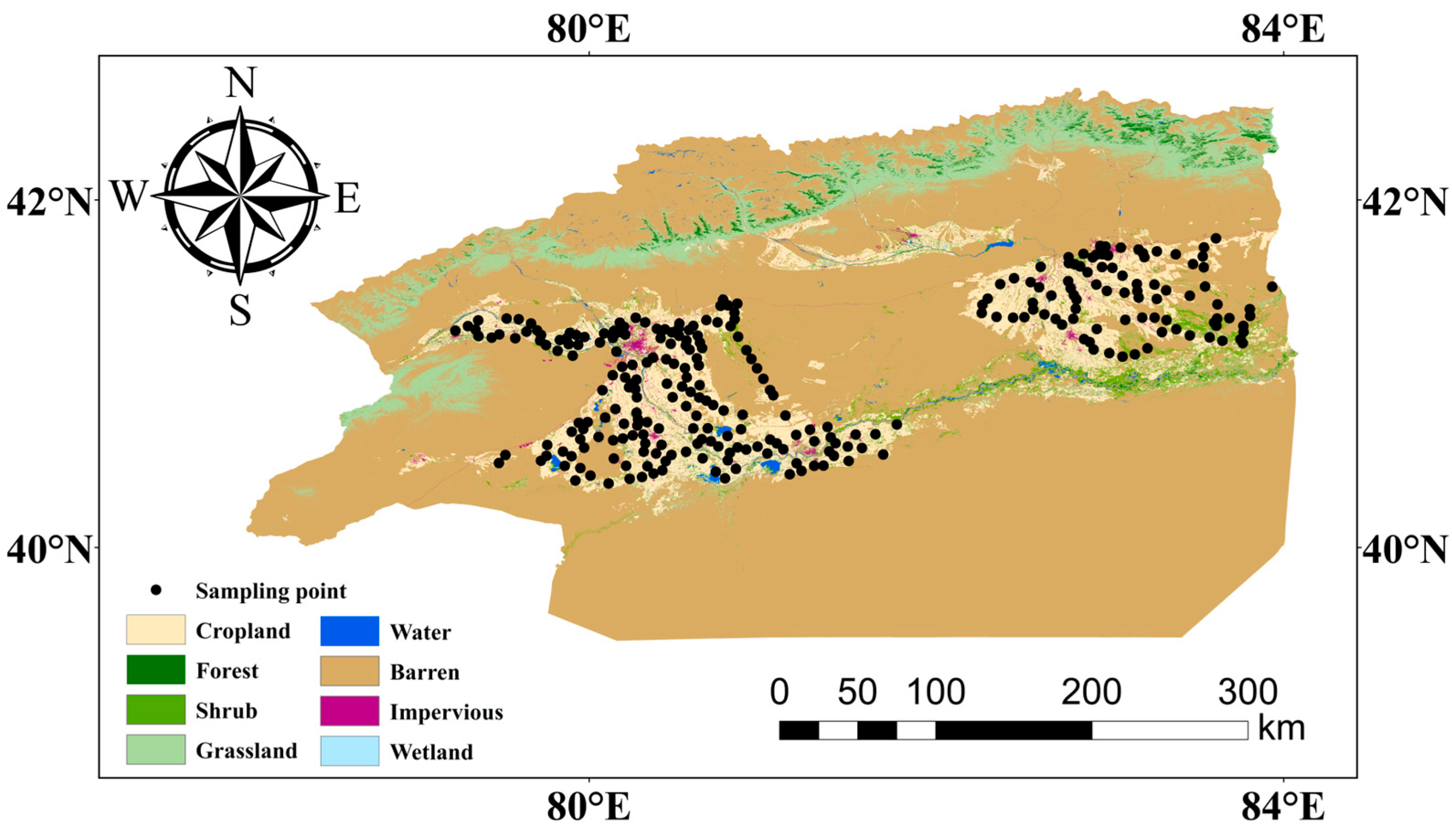
To obtain sufficient and effective EC samples, two rounds of sampling were conducted in July and October of 2023. July was chosen for sampling because the high temperatures in the Aksu region at this time promote active vertical movement of soil salts, which helps reveal the dynamic changes in soil salinization. October, on the other hand, coincides with the autumn irrigation break after crop harvest, when irrigation activities on the farmland have largely ceased, and soil moisture movement is reduced. During this period, surface soil salts accumulate significantly due to evaporation, clearly reflecting the salt accumulation characteristics during the non-irrigation period [17]. To ensure representative sampling and comprehensive spatial coverage, we employed a spatial distribution strategy combining Stratified Sampling with a Transect Design, establishing a total of 276 sampling points, whose spatial locations were kept identical for both sampling campaigns to ensure temporal comparability. Specifically, we stratified the area into a “Core Oasis Cropland” and an “Oasis–Desert Transition Zone,” allocating 210 and 66 points, respectively. Spatially, these points were arranged into two primary east–west transects, with all points spaced over 1 km apart to ensure their independence, as shown in Figure 2. At each predetermined location, precisely recorded using a handheld GPS device, we first collected a composite surface sample (0–10 cm), using a five-point method (10 m spacing). Subsequently, at the center point, we conducted vertical profile sampling using a 5 cm diameter stainless-steel soil auger to collect soil from six distinct depth layers, namely 0–10 cm, 10–20 cm, 20–40 cm, 40–60 cm, 60–80 cm, and 80–100 cm, with each sample weighing approximately 500 g. After collection, the soil samples were quickly placed into numbered, sealed plastic bags for preservation and then transported to the laboratory for processing. The laboratory processing followed the following steps strictly: (1) All of the samples were air dried in the laboratory. (2) Fully dried soil samples were ground into powder and passed through a 0.5 mm sieve to remove impurities. (3) The powdered soil samples were accurately weighed and placed in numbered conical flasks to prepare a solution with a soil-to-water ratio of 1:5. (4) The prepared solution was thoroughly shaken and then left to stand for 24 h. (5) Finally, the solution was filtered using filter paper, and the upper clear liquid was used for measuring its EC.

2.2.3. Environmental Covariates

To enhance the spatial resolution of solar-induced chlorophyll fluorescence (SIF), this study utilized a Stacking ensemble learning framework, trained using a suite of twenty-nine environmental covariates, as shown in Table 1. All of the covariates were acquired and preprocessed using the Google Earth Engine (GEE) platform. The standardized preprocessing workflow included: cloud and cloud shadow masking for optical imagery (MODIS) based on their quality assessment (QA) bands; temporal aggregation of time-series data (e.g., ERA5-Land) into monthly composites; and spatial resampling of all the layers to a uniform 30 m resolution via bilinear interpolation. The covariates consisted of two distinct types: (1) existing data products retrieved directly from the GEE data catalog, and (2) spectral indices computed from raw optical bands within the GEE environment. Specifically, topographical covariates were derived from the ASTER GDEM product, including the Digital Elevation Model (DEM), Topographic Position Index (TPI), and Topographic Wetness Index (TWI). Climate variables were sourced from the TerraClimate (precipitation, PET, and Climatic Water Deficit) and ECMWF ERA5-Land (three soil temperature layers: ST1–ST3) datasets. The soil substrate was characterized by the Depth to Bedrock (DTB) variable from SoilGrids. Finally, a range of biological and land surface state covariates, such as the NDVI, EVI, SIWSI, and the LST, DDI, and CBN, were computed.

2.2.4. MOD17A2 GPP

Gross Primary Productivity (GPP), the total amount of carbon fixed by vegetation through photosynthesis, is a core indicator of the ecosystem carbon cycle. As GPP and SIF are both closely related to photosynthetic activity, GPP is commonly used as a key reference for validating SIF products [43]. In this study, GPP was primarily used to assess the accuracy and reliability of the downscaled SIF product. To this end, 8-day composite GPP data from the MOD17A2H v061 product were utilized. To ensure its spatial consistency with other covariates, this dataset was resampled to a 30 m spatial resolution, effectively supporting the validation of the SIF downscaling model in this study.

2.2.5. Land Use Data

In this study, we employed the 30 m annual land cover datasets of China (CLCD) from 2023, which were generated using over 335,000 Landsat images on the Google Earth Engine platform. The CLCD is a Landsat-derived land cover product that offers temporally consistent classification maps from 1985 to 2023, developed using a random forest classifier, trained with samples from China’s Land Use/Cover Datasets (CLUD), time-series satellite data, Google Earth, and other auxiliary sources. The 2023 version of the CLCD dataset has been released in Cloud Optimized GeoTIFF format, facilitating efficient access and spatial analysis [44].
The CLCD data were used to classify the sampling points into vegetated and non-vegetated areas. This classification step was essential, as certain sampling locations lacked vegetation coverage, which could interfere with the interpretation of vegetation-related indicators, such as SIF. By integrating CLCD land cover information, we ensured that the analysis of SIF–soil salinity relationships was restricted to ecologically relevant zones, where vegetation was present and photosynthetic activity could be reliably assessed. To accurately distinguish between vegetated and non-vegetated sample points, we employed the 2023 version of the China Land Cover Dataset (CLCD), which classifies the land surface into nine categories: cropland, forest, shrub, grassland, water, snow/ice, barren land, impervious surfaces, and wetland. Based on their ecological characteristics and potential for supporting photosynthetic activity, cropland, forest, shrub, grassland, and wetland were categorized as vegetated areas. These land types typically sustain active vegetation cover and are suitable for analyses involving SIF. In contrast, water bodies, snow/ice, barren land, and impervious surfaces were classified as non-vegetated areas, due to their lack of substantial vegetation or photosynthetic function. This classification enabled us to mask ecologically irrelevant pixels and ensure that the correlation analysis between SIF and soil EC focused exclusively on regions where vegetation was present and photosynthetically active. This step was crucial for enhancing the biological interpretability and spatial accuracy of the results.

2.3. Methods

2.3.1. Stacking-Based Downscaling Strategy

In this study, we employed the Stacking ensemble learning method for downscaling the prediction of solar-induced fluorescence (SIF). The core principle of the Stacking ensemble is to combine predictions from multiple heterogeneous base learners to achieve superior performance over any single model [45]. The framework in this study specifically integrates three powerful regressors as base models, namely Random Forest, XGBoost, and CatBoost, and employs linear regression as the meta-model to generate the final prediction. This strategy is designed to leverage the unique, complementary strengths of each algorithm: Random Forest excels at handling high-dimensional data and feature interactions; XGBoost is highly effective at capturing complex nonlinear relationships; and CatBoost is robust when processing categorical features and mitigating gradient bias [46]. By synergizing these complementary models, the Stacking framework effectively reduces the overfitting risk inherent to any individual model, thereby significantly enhancing the stability, generalization ability, and overall accuracy of the final prediction [47]. In addition, the Stacking model performs well in integrating multiple environmental covariates. By incorporating six categories of environmental covariates, including climate, parent material, topography, hydrology, biology, and climate-environmental factors, the Stacking model is able to comprehensively consider the impact of various factors on SIF, enabling more refined spatial predictions.
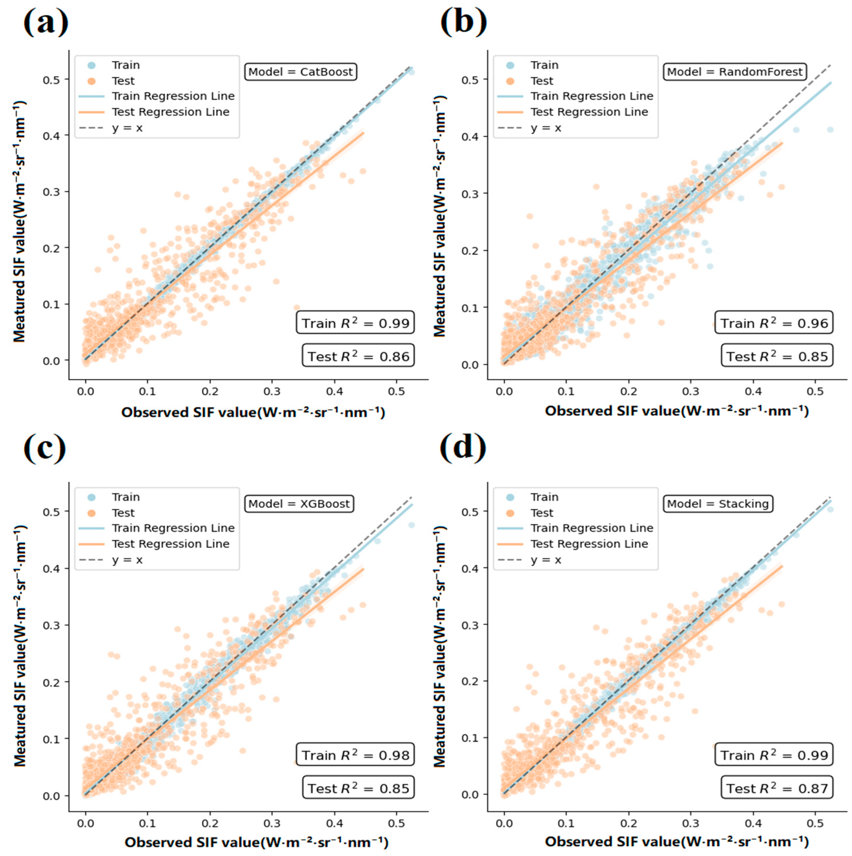
In this study, we conducted a comprehensive assessment of several machine learning models for predicting SIF, using environmental covariates from July and October 2023 and GOSIF data. To ensure a rigorous and transparent comparison, the dataset was first partitioned into an 80% training set for model development and a 20% independent test set for the final, unbiased validation. We compared three primary models, namely Random Forest, XGBoost, and CatBoost, each of which was systematically optimized using a 5-fold cross-validated randomized search, based on the training data. This process focused on the most influential hyperparameters, while others were kept at their robust default settings. For the Random Forest model, the tuning focused on key structural parameters; the optimization resulted in a final configuration with 500 trees (n_estimators), a maximum depth (max_depth) of 20, and a minimum leaf size (min_samples_leaf) of 2. Similarly, the XGBoost model’s optimization targeted parameters controlling its boosting process and complexity. The best-performing model used a learning rate (learning_rate) of 0.05, 600 estimators (n_estimators), a max_depth of 6, and a subsample ratio of 0.8. For the CatBoost model, the tuning led to an optimal setup with 1000 iterations, a learning rate (learning rate) of 0.1, a tree depth (depth) of 6, and an L2 regularization (l2_leaf_reg) value of 3. Finally, these three optimized models were integrated as base learners into a two-level Stacking Regressor ensemble, with linear regression serving as the meta-model. Crucially, the Stacking Regressor was implemented with an internal 5-fold cross-validation to train its meta-model on out-of-fold predictions from the base learners. This critical step ensures the meta-model’s training is unbiased, enabling it to more accurately learn how to fuse the predictive strengths of the different models, thereby significantly improving the final model’s prediction accuracy and generalization ability. This comprehensive approach was chosen because these advanced models are exceptionally capable of handling the complex nonlinear relationships and high-dimensional data characteristic of environmental science [48]. As shown in Figure 3, the CatBoost model demonstrates relatively robust performance, with an R2 of 0.86, indicating good fitting ability. XGBoost and Random Forest are similar, both with an R2 of 0.85. The Stacking Regressor model, as an ensemble learning method, significantly enhances prediction performance by combining the strengths of the three base models mentioned earlier. Specifically, the R2 value is 0.87, outperforming the individual models. This result indicates that the Stacking Regressor has a significant advantage by leveraging the predictive capabilities of different models, enabling it to more accurately capture the complex relationship between SIF and environmental covariates [49].

2.3.2. SIF-Driven Soil EC Estimation

This study designed three sub-experiments for SIF data with different spatial resolutions (0.05°, 0.005°, and 30 m) to explore whether higher resolution SIF data can improve the accuracy of soil EC estimation. By systematically analyzing the response relationship between SIF products with different resolutions and crop yield, the study evaluates the impact of the data spatial scale on soil salinity monitoring. Additionally, the study validated the correlation between monthly SIF and soil EC, based on temporal data, and established a linear regression model to quantify the strength of their association. To further explore the potential of multi-source data, three machine learning algorithms, namely Random Forest (RF), Classification and Regression Trees (CART), and XGBoost, were used to construct a collaborative SIF–EC prediction model, aiming to identify the optimal feature set for higher estimation accuracy.

2.3.3. Overall Process

The overall research process is shown in Figure 4. First, we integrated GOSIF data, MODIS imagery, GPP data, TerraClimate data, SoilGrids data, ECMWF ERA5-Land data, ASTER GDEM data, and field-measured soil EC data, followed by data preprocessing. Then, a Stacking-based regression method was used to downscale the GOSIF data, generating a 0.005° SIF dataset. Subsequently, the 0.005° SIF data and environmental covariates were used to generate a 30 m SIF dataset. During the model construction phase, key environmental variables were selected through the use of correlation analysis. Linear regression was then used to validate the relationship between SIF data and soil EC. Various machine learning algorithms, including Random Forest (RF), XGBoost, and Classification and Regression Trees (CART), were applied to model and compare different SIF datasets, with varying resolutions. The performance of each model was evaluated using the coefficient of determination (R2) and root mean square error (RMSE), based on the validation data. To assess the applicability of SIF products with different resolutions for soil EC estimation, we used the July and October sample points collected in the Aksu region, combining SIF and environmental covariates to generate SIF–EC models at different depths. By comparing the accuracy of the models generated using different environmental covariates and SIF, we identified the optimal environmental covariates, and then generated SIF–EC models for each depth.

3. Results

3.1. Generation and Evaluation of Downscaled SIF

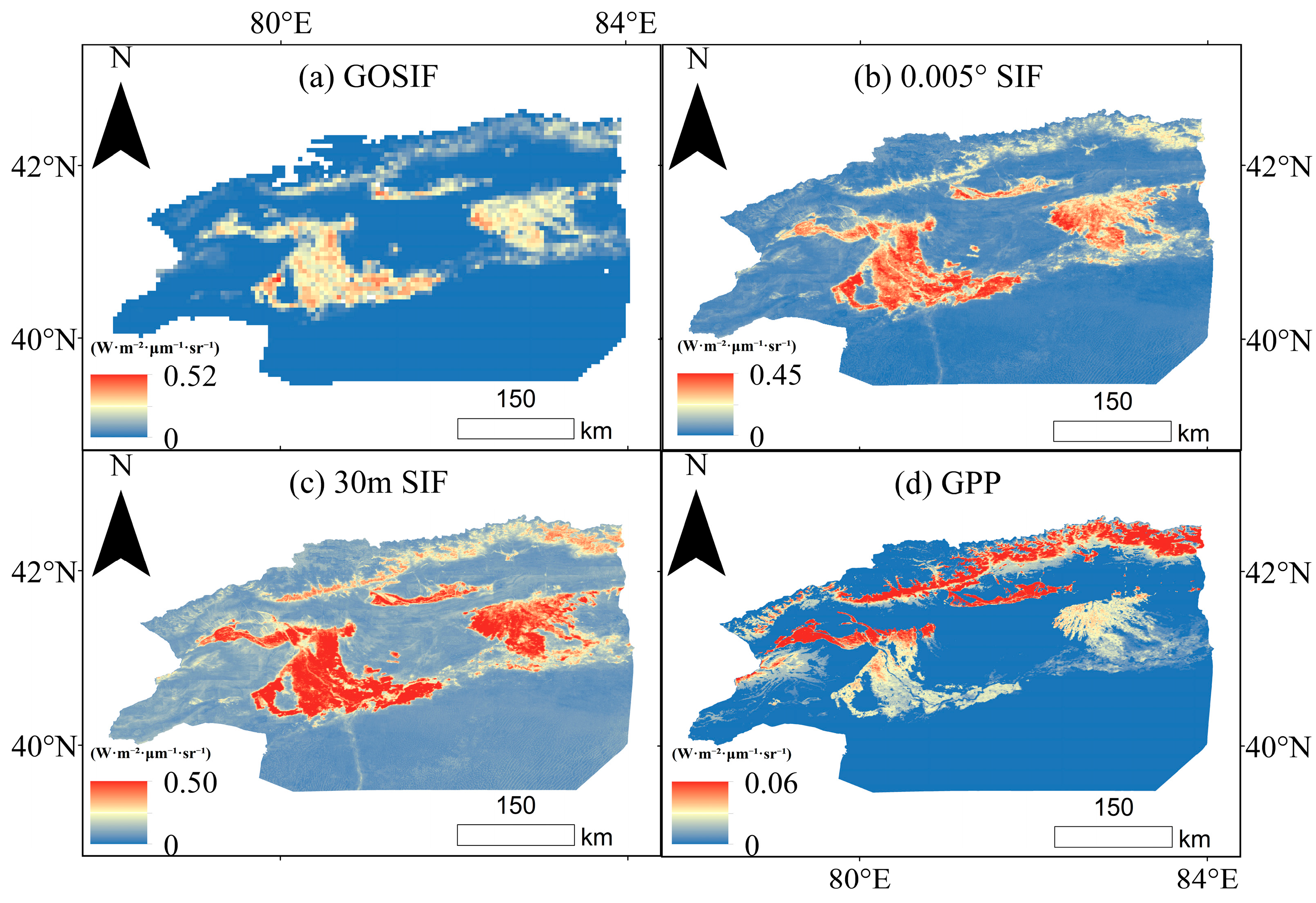
To improve the spatial resolution of SIF, this study employed a multi-step downscaling method. First, using environmental covariates with a 0.05° resolution and existing SIF data, the Stacking model was applied to generate SIF data at a 0.005° resolution. The Stacking ensemble learning model, by integrating the strengths of multiple base learners, has been proven to have significant advantages in regard to handling complex nonlinear relationships and large-scale data [50]. This stage aims to refine the spatial variability of SIF to better capture the dynamics of surface vegetation photosynthesis. Subsequently, by combining the 0.005° resolution covariates and the generated SIF data, the same downscaling technique was applied to enhance the SIF resolution to 30 m, in order to match the ground observation sample points. The downscaled SIF is shown in Figure 5. This high-resolution SIF generation not only preserves the characteristics of large-scale environmental influences, but also reflects the variations in vegetation photosynthesis at the microscale. Previous studies have shown that the relationship between SIF and GPP can effectively reflect vegetation photosynthetic efficiency and the carbon cycle in ecosystems, as shown in Figure 6. The downscaled SIF product exhibits high spatial consistency with the original GOSIF product and demonstrates a strong correlation with Gross Primary Productivity (GPP). This indicates that the developed high-resolution SIF product not only retains the accuracy of the original data, but also provides a more detailed reflection of spatial variations in vegetation photosynthesis [51,52].

3.2. Correlation Analysis Between SIF and Soil Salinity

By analyzing the correlation between soil EC at different depths and SIF, we aim to reveal the response mechanisms of SIF across soil layers and further investigate the influence of soil depth on SIF signals. The study of soil EC at varying depths is essential because the physical and chemical properties of soil vary considerably with depth. Differences in the distribution of moisture, salinity, and other components between shallow and deep soil layers can significantly affect the SIF response.
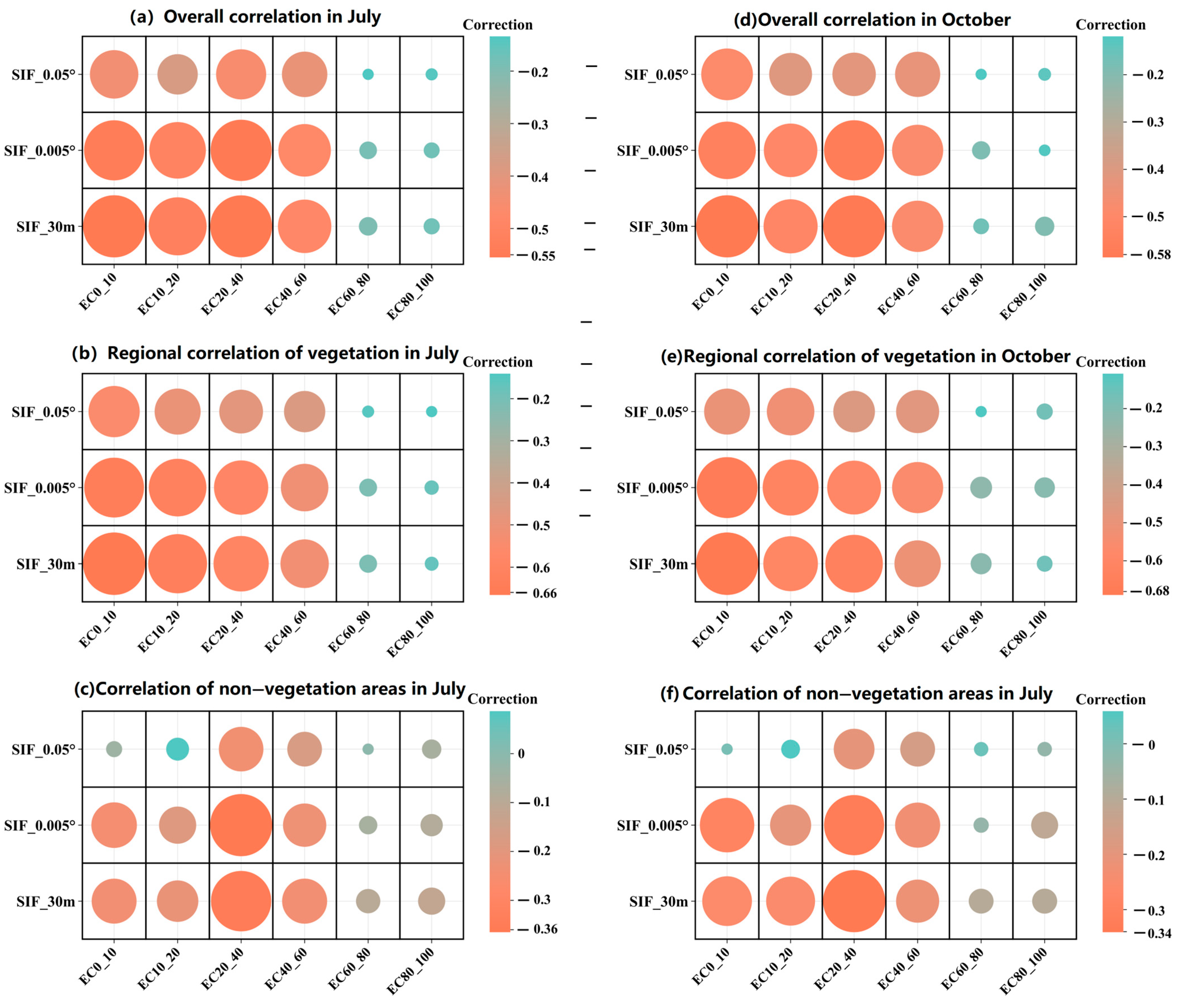
Figure 7 presents the correlation analysis between SIF and soil EC at different spatial resolutions and soil depths for July and October 2023. A pronounced negative correlation is observed between SIF and EC within the 0–60 cm shallow to mid-depth soil layers, whereas this correlation weakens considerably in deeper soils below 60 cm. The negative correlation is particularly evident in vegetated areas, indicating that soil salinity in the upper layers exerts a stronger inhibitory effect on vegetation photosynthesis, which is effectively captured by the SIF signal. In contrast, in non-vegetated regions, where active photosynthetic processes are absent or minimal, SIF signals are weaker and exhibit a less consistent response to soil salinity stress, resulting in generally lower correlations and more spatially scattered patterns.
From a temporal perspective, the correlation between SIF and soil EC in October is generally higher than in July. This suggests that during the later stages of plant growth or periods of cumulative drought stress, photosynthetic activity tends to stabilize, allowing SIF to more effectively capture and reflect the long-term impact of soil salinity on vegetation. In contrast, July corresponds to the peak of the vegetation growth phase, during which photosynthesis is strongly influenced by multiple environmental factors, such as temperature, moisture, and nutrient availability. As a result, the SIF response to salinity may be masked by short-term physiological fluctuations, thereby weakening its correlation with soil EC.
It is worth noting that significant differences exist in the correlation performance among SIF products with different spatial resolutions. High-resolution products (e.g., SIF_0.005° and SIF_30 m) consistently exhibit stronger correlations across various regions and time periods, particularly in vegetated areas, where they show higher negative correlation coefficients with shallow soil EC. This may be attributed to the ability of high-resolution data to more precisely capture the fine-scale spatial distribution of surface vegetation, thereby enhancing the sensitivity of SIF to spatial heterogeneity in soil salinity. In contrast, low-resolution SIF products may be subject to mixed-pixel effects, where signals are influenced by multiple land cover types within a single pixel. This reduces their ability to accurately detect fine-scale variations in soil salinity.
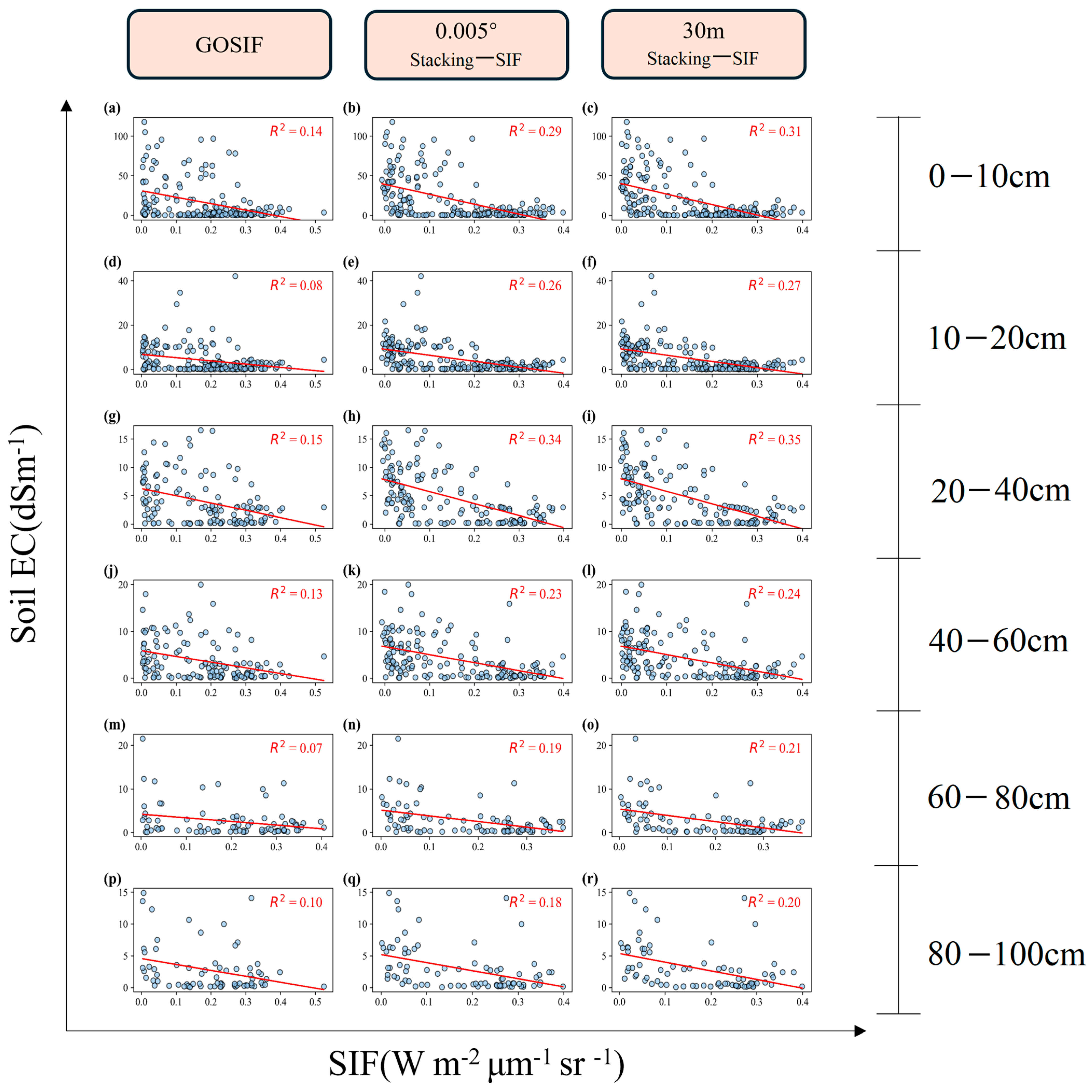
In addition, as shown in Figure 8, this study constructed linear regression models for soil EC using SIF data at different resolutions (GOSIF, 0.005° Stacking–SIF, and 30 m Stacking–SIF), and explored the impact of resolution on modeling effectiveness by comparing the fitting results of different models. The results show that increasing the SIF resolution significantly enhances the representation of soil EC, with the 30 m resolution model showing the highest R2 values across multiple soil depth ranges, particularly with an R2 of 0.35 at the 20–40 cm depth. However, we observed that the model’s predictive accuracy remained relatively low. This is likely because the underlying relationship between SIF and soil EC is fundamentally nonlinear, a characteristic that is clearly visible in the scatter plots shown in Figure 8. Therefore, we plan to incorporate additional environmental covariates to assist in improving the model’s performance. A negative correlation between SIF and soil EC was observed, reflecting the characteristics of high-fluorescence regions, where vegetation health is good and soil salinity is low. These findings indicate that high-resolution SIF data have significant potential for soil salinization prediction, particularly in monitoring shallow soils, where it can significantly improve model prediction accuracy and enhance the spatial detail of soil salinization monitoring.

3.3. SIF-Based Soil EC Estimation

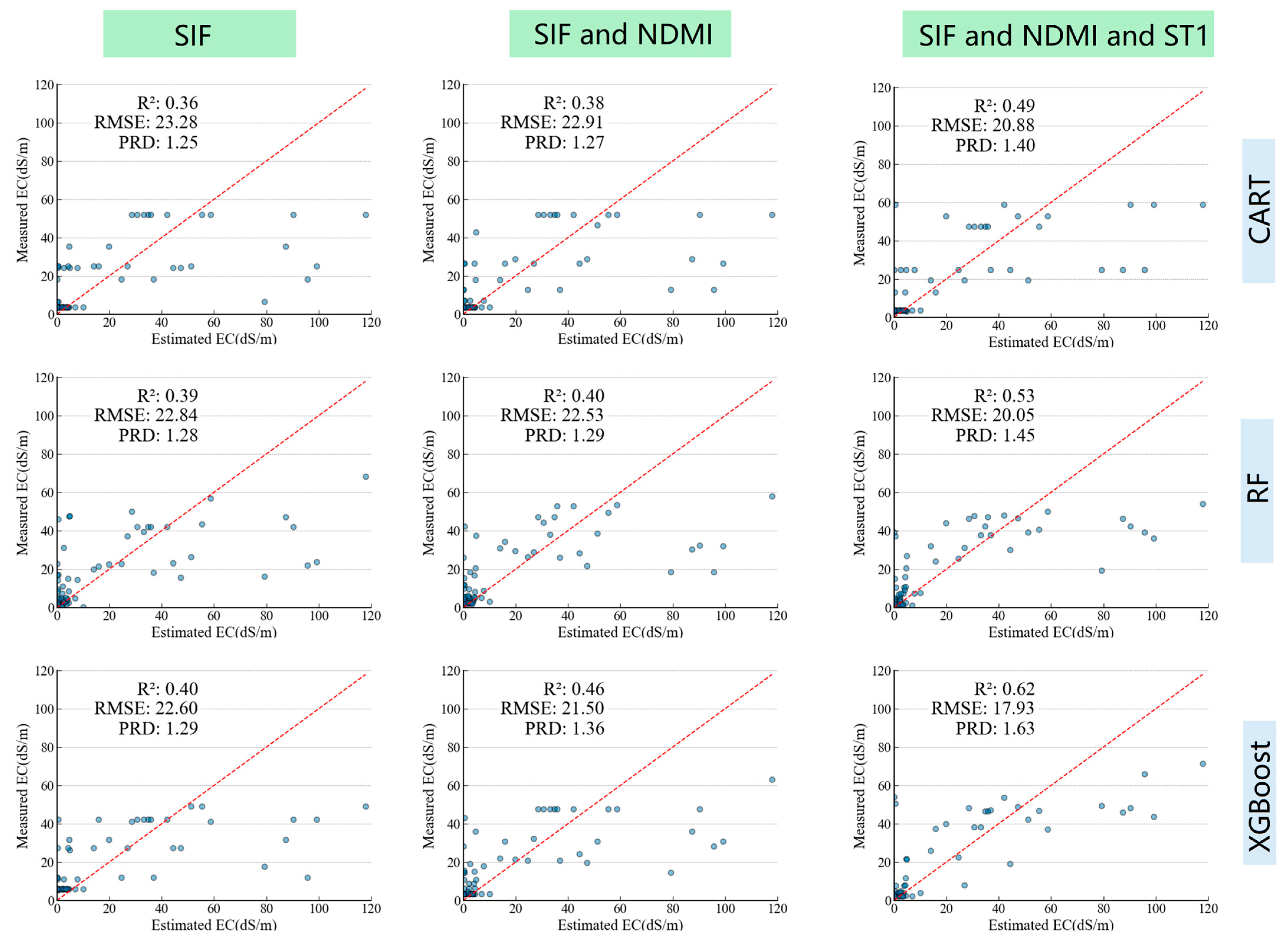
The unique role of the SIF index in soil EC estimation primarily lies in its ability to directly reflect vegetation photosynthetic efficiency, thereby indirectly indicating the spatial distribution of soil salinity. However, when using only the SIF index or traditional environmental covariates, the model’s predictive ability is somewhat limited. Relying solely on the SIF index makes it difficult for the model to fully capture terrain and spatial background information, while using only traditional environmental covariates lacks a direct reflection of the vegetation’s physiological state [53]. Therefore, a model combining the SIF index and environmental covariates can integrate terrain, spatial background, and vegetation physiological state information, significantly improving the model’s prediction accuracy and stability. As shown in the Figure 9, the model (i) combines the SIF index with multiple environmental covariates, achieving an R2 of 0.62, an RMSE of 17.93 dS/m, and a PRD of 1.63, outperforming other models. This result first indicates that the combination of SIF and other environmental covariates is superior to using SIF alone, suggesting that incorporating more independent variables effectively improves the accuracy of soil EC estimation, which has significant practical implications. Furthermore, compared to using vegetation indices alone, the combination of SIF and environmental covariates significantly improved the R2 and reduced the RMSE, further demonstrating the advantages of multi-source data fusion. Additionally, the XGBoost model performed better than the Random Forest (RF) and Classification and Regression Trees (CART) models in terms of soil EC prediction, showcasing its superiority in handling complex nonlinear relationships and high-dimensional data.
This study further considers the vertical stratification characteristics of soil EC and optimizes the model by using differentiated combinations of environmental covariates at different depth layers. Previous studies have shown that the spatial distribution of soil EC exhibits significant depth variations, and environmental covariates at different depths have a significant impact on model accuracy [54]. Differentiated combinations of environmental covariates were used to optimize the model at different depth layers, with the selected environmental covariates determined by the model accuracy. As shown in Table 2, for surface soils (0–10 cm) in July, the model primarily used NDMI and ST1 as dominant factors; at the 10–20 cm depth, S13 and DEM were selected as key covariates; for the 20–40 cm mid-layer soil, S13 and PRET were introduced to reflect salt infiltration dynamics; at the 40–60 cm depth, ST1 and DEM were combined to capture the effects of parent material and topography; and for deeper soils (60–80 cm), the combination of NDMI and VSW1 effectively characterized the downward movement of salt through leaching. For the 80–100 cm depth, the model predicted soil EC using the combination of NDMI and ST1. In October, the main environmental covariates were EVI and SI. Meanwhile, we found that the 30 m resolution SIF had the highest accuracy during modeling, as shown in Figure 10. In July, the SIF–EC model at the 0–10 cm depth had the highest accuracy, with R2 = 0.62, while in October, the SIF–EC model at the 40–60 cm depth exhibited the highest accuracy, with R2 = 0.73.
Furthermore, the results seem to indicate that the model exhibits a distinct saturation effect in its EC estimation, which becomes significant at EC values exceeding approximately 40 dS/m. We speculate that this phenomenon may be primarily attributed to the inherent physiological tolerance limits of vegetation under extreme salinity stress; in such hypersaline conditions, plants may typically surpass their salinity tolerance thresholds and become insensitive to further increases in soil EC.

3.4. Soil EC Distribution

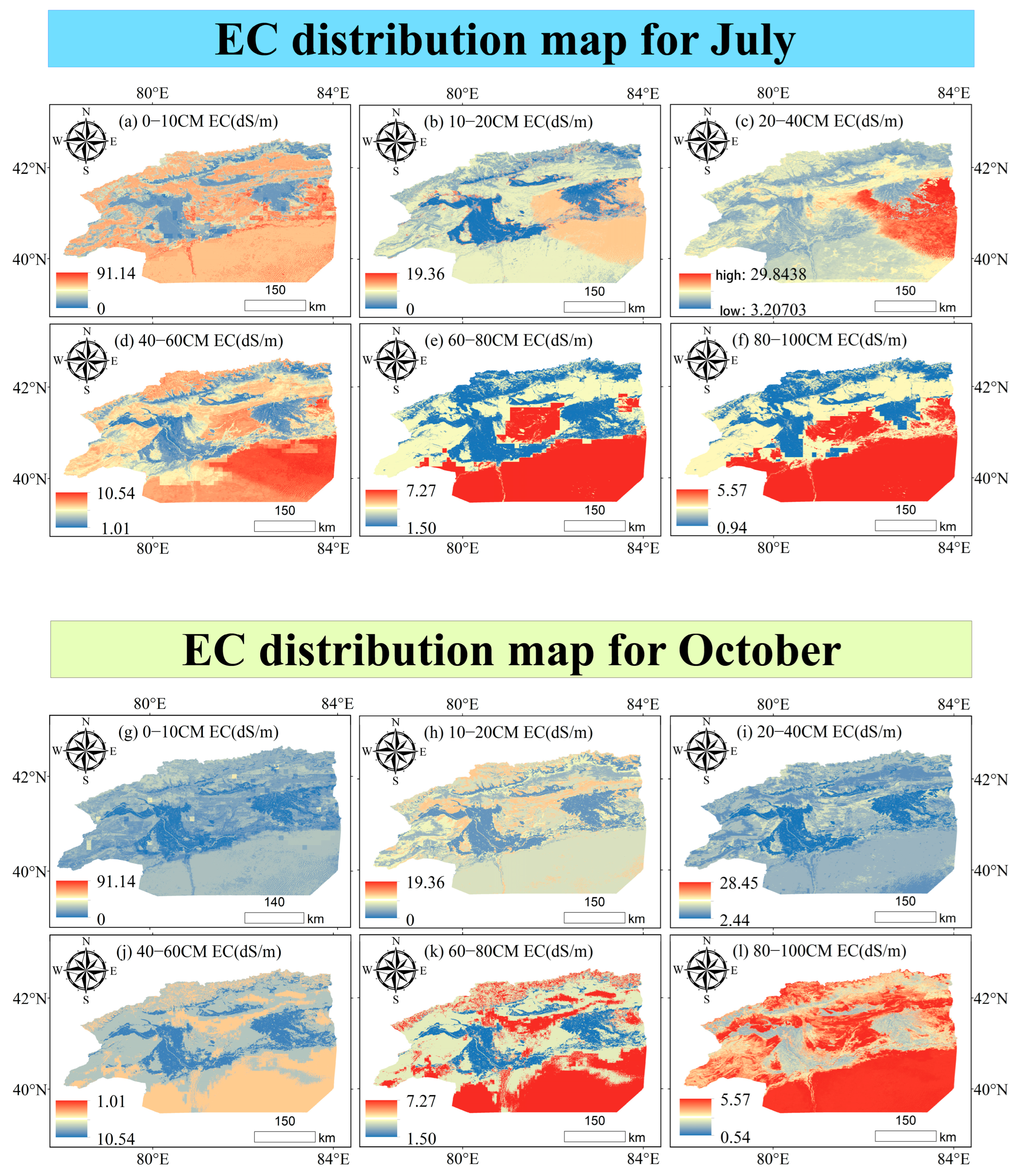
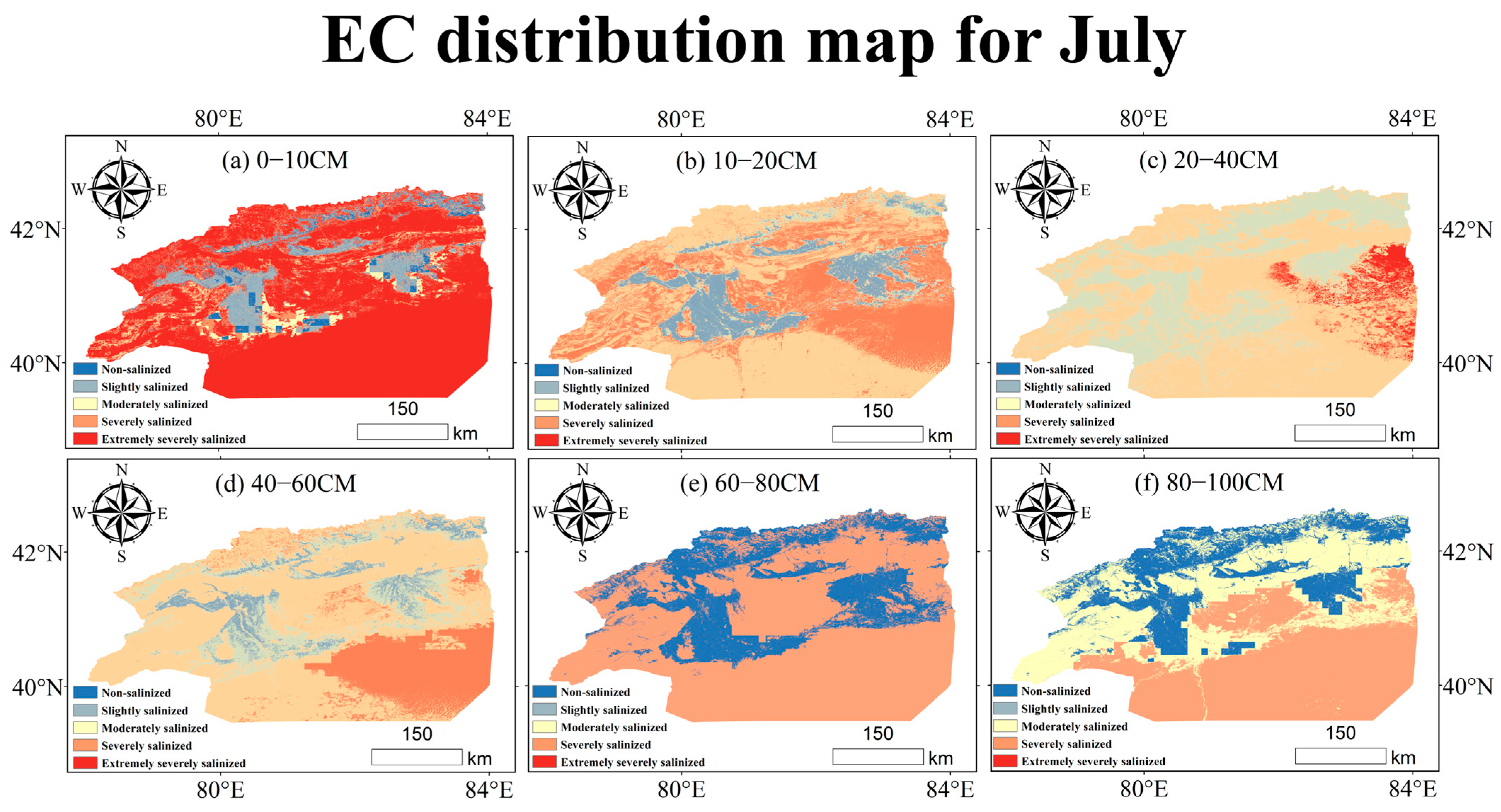
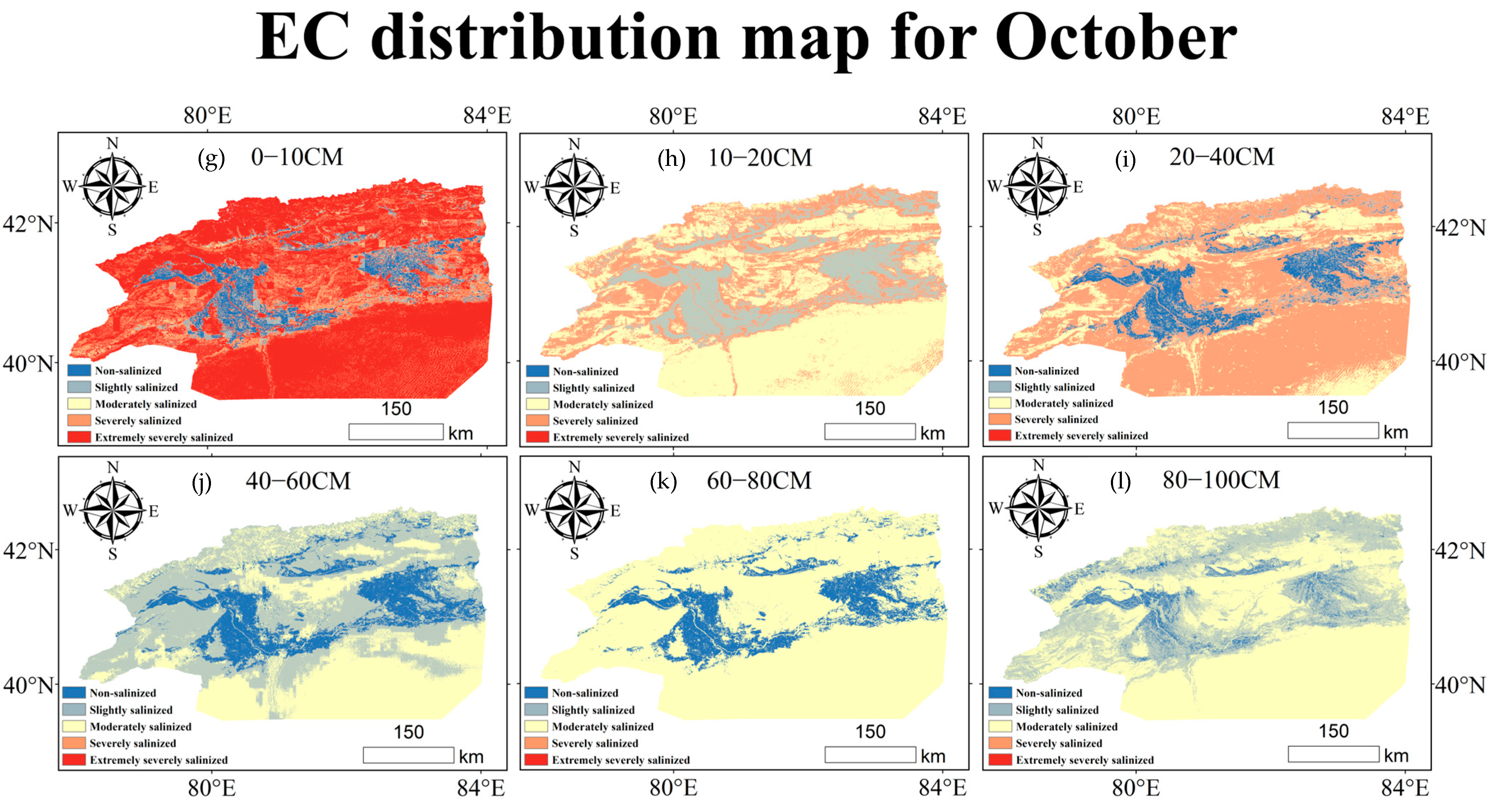
The SIF–EC model, constructed based on the Stacking ensemble method, by integrating multi-source remote sensing data and ground-measured samples, generated spatial distribution maps of soil EC at different depths (0–10 cm, 10–20 cm, 20–40 cm, 40–60 cm, 60–80 cm, 80–100 cm) for the Aksu region in July and October 2023. As shown in Figure 11, in terms of the temporal dimension, the soil EC values in July were generally higher than in October, with the highest EC values observed at the surface layer (0–10 cm). This may be due to the high temperatures and longer daylight hours in July, which led to intense soil moisture evaporation, causing salt to migrate upwards through capillary action and accumulate at the surface, thereby increasing the EC values. In terms of vertical patterns, the results indicate that the most severe salinization occurred in the surface soil (0–10 cm). A general pattern of lower salinization was observed in deeper layers relative to the surface, with the exception of a secondary high-salinization layer found at the 20–40 cm depth. This may be due to this depth being in an active zone of soil moisture movement, where it both receives salts from surface infiltration and is influenced by capillary rise from groundwater [55]. Additionally, the 20–40 cm layer often exhibits texture changes (such as clay layers), which hinder the further downward movement of salts, causing temporary salt accumulation at this depth [56]. In terms of spatial patterns, regional differences are significant: the southern part of Kuche County, the southeastern part of Xinhe County, the northern part of Shaya County, the southwestern part of Wensu County, and the western part of Wushi County are characterized as areas of mild salinization; the northern part of Awati County, the southern part of Baicheng County, and the central part of Wensu County are classified as areas of moderate salinization; while the southeastern part of Shaya County and other areas exhibit features of severe salinization. Overall, the Aksu region shows high salinity levels [57].

4. Discussion

The Stacking–SIF model at a downscaled resolution of 30 m achieved acceptable soil EC estimation accuracy at the field scale. With the support of other environmental covariates, the combined model demonstrated R2 values ranging from 0.53 to 0.67 across models at six different depths in both July and October. Despite these results, several uncertainties may limit improvements in soil EC estimation performance in this study. The main sources of uncertainty include the proposed SIF downscaling strategy, errors in the soil EC samples, and uncertainties associated with the data. Additionally, the potential of refined SIF products for use in soil salinity detection is further discussed.

4.1. Validation of Downscaled SIF Results

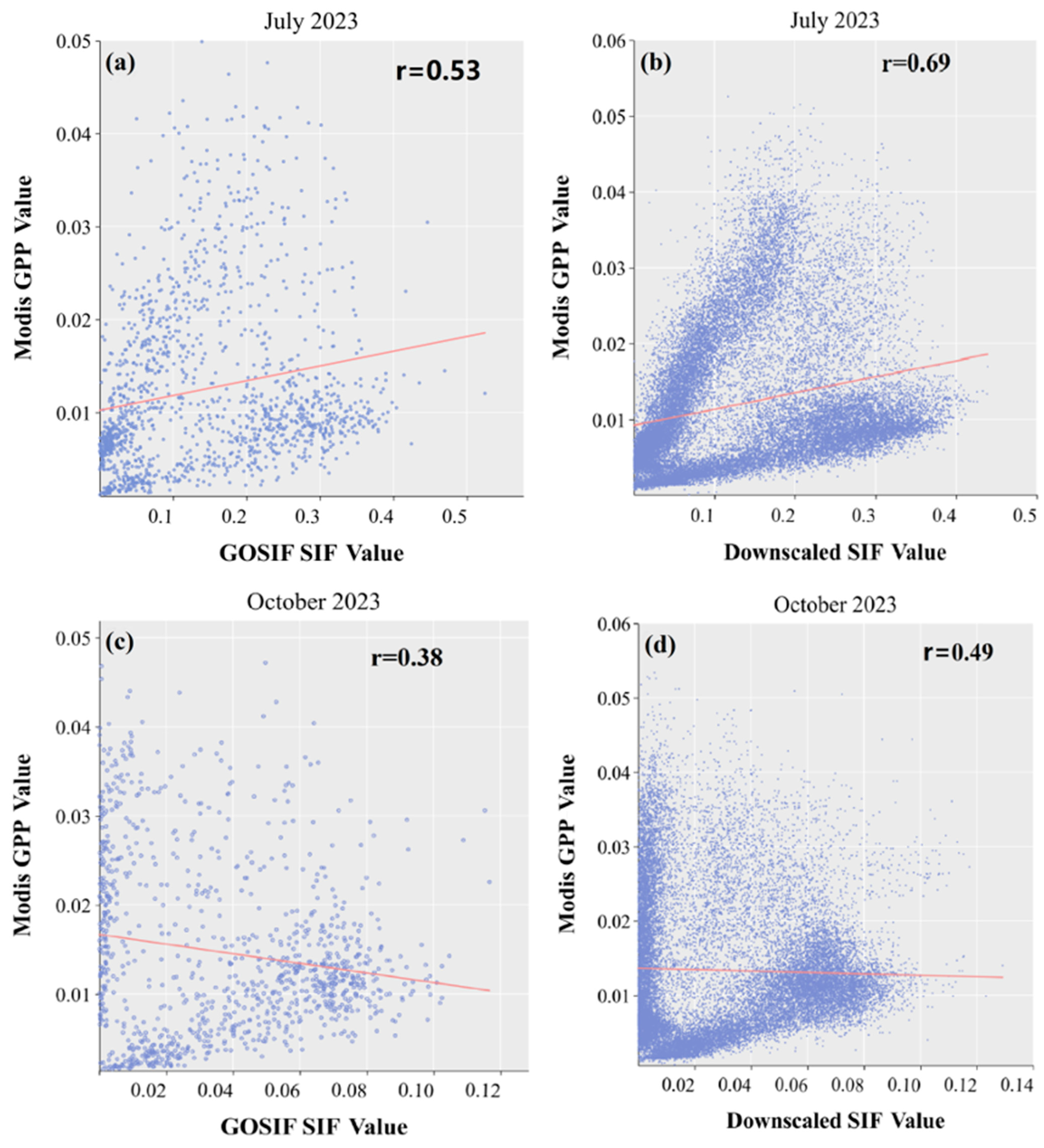
Numerous experimental studies have shown a significant linear correlation between SIF and Gross Primary Productivity (GPP) [58]. SIF signals reflect the absorption and release of light energy during the photosynthetic process in plant leaves, while GPP represents the total amount of carbon fixed by plants. Therefore, the two are closely related through their physical processes [59]. To systematically assess the reliability of the downscaling results, this study selected MODIS GPP data for July and October as a validation benchmark. The data were resampled to a 0.05° spatial resolution to match the GOSIF data, followed by a correlation comparison between the original GOSIF data, the downscaled SIF data, and GPP. As shown in Figure 12, the comparison reveals that in July 2023, the downscaled SIF data exhibited the strongest correlation with GPP (r = 0.69), which was stronger than that of the original GOSIF data. However, we observed two clearly separate trend lines in Figure 12b, and we infer that the primary reason for this is the mixture of different vegetation types (biomes) within the study area. Specifically, the steeper, denser trend line likely represents croplands or grasslands, where the coupling between SIF and GPP is very tight and linear. In contrast, the other, relatively flatter trend line likely represents forest ecosystems, whose complex canopy structure affects the transmission of the SIF signal (e.g., through signal re-absorption by the upper canopy), thereby exhibiting an SIF–GPP relationship different from that of croplands. Additionally, the correlation in July was significantly better than in October, and this difference may be attributed to the reduced SIF signal intensity, due to the weakening of vegetation photosynthesis in the autumn [60]. We also performed a correlation analysis between the original GOSIF data and the downscaled SIF data. As shown in Figure 13, the downscaled SIF results were resampled to the same spatial resolution (0.05°) as the original SIF data. A scatter plot was generated by comparing the original SIF values (GOSIF) with the resampled downscaled SIF values. The comparison yielded the correlation coefficient (r) between the downscaled SIF and GOSIF. The results showed a strong correlation between the downscaled SIF data and GOSIF, with the highest correlation in July (r = 0.95). This result validates the effectiveness of the downscaling method in improving the spatial resolution of SIF data, while retaining the original information. It should be noted that these results remain subject to biases and uncertainties: (i) MODIS GPP itself carries algorithmic and forcing-data uncertainties that can introduce spatiotemporally dependent bias; (ii) resampling and scale mismatch processes smooth spatial variability and may introduce shared operator and spatial autocorrelation effects that inflate correlations; (iii) under high light or stress, the responses of SIF yield and carbon assimilation can partially decouple, contributing to seasonal differences; and (iv) the downscaling procedure may inherit systematic errors from BRDF, sun–sensor geometry, and atmospheric correction. Accordingly, we interpret the downscaling effect as evidence of enhanced spatial detail with the overall information preserved and recommend that future work quantify uncertainty via rank-based correlations, biome-stratified analyses, and spatial block resampling, alongside comparisons with flux tower GPP, where available.

4.2. Spatial Distribution of Soil EC

In this project, soil salinization levels were classified into five categories based on the measured conductivity (EC1:5): non-salinized, lightly salinized, moderately salinized, heavily salinized, and extremely heavily salinized. The classification criteria are shown in Table 3.
Subsequently, we reclassified the soil EC distribution maps generated by the SIF–EC model into soil salinity level distribution maps. As shown in the Figure 14, the surface soil (0–10 cm) in the Aksu region exhibits severe salinization. As the soil depth increases, the degree of soil salinization gradually decreases. This phenomenon can be attributed to evaporation and capillary action at the soil surface, causing salts to accumulate at the surface, while deeper soils are less affected [54]. Our SIF–EC model further reveals a distinct spatial heterogeneity in soil salinity across the region, with its results clearly identifying a significant high-salinity zone in the southeastern part of Shaya County. This zone contrasts sharply with a low-salinity corridor that we identified stretching from southern Kuche County to western Wushi County. This level of spatial detail, particularly in transitional areas like central Wensu County, showcases the model’s enhanced sensitivity to localized salinity drivers. We interpret this pronounced spatial pattern as a direct reflection of regional differences in irrigation management and the underlying hydrogeological conditions. The scientific foundation for our SIF–EC model is based on the strong physiological principle linking soil salinity to vegetation stress and, consequently, to photosynthetic function. High soil EC impairs photosynthesis, leading to a detectable decrease in the SIF signal, often before visible signs of degradation (e.g., a decline in NDVI) occur. Therefore, the spatial variations in SIF captured by our model serve as a highly sensitive proxy for the underlying salinity stress. The low-salinity corridor identified by our model aligns with areas known for having more efficient irrigation infrastructure, while we hypothesize that the high-salinity hotspot in southeastern Shaya County results from less effective water management. This interpretation is consistent with previous studies that have broadly linked improper irrigation to severe salinization in arid regions [61]. Furthermore, the SIF–EC model effectively captures the vertical stratification of salinity. Our results show a much steeper gradient from surface (0–10 cm) to deeper soils within the identified high-salinity zones compared to the low-salinity areas. This finding provides clear visual evidence for the significant spatial differences in salt profiles across the region and suggests that in areas like southeastern Shaya, capillary action is a dominant driver [54], a process our model visualizes with high clarity. The model also sharply delineates the salinity differences between the late growing season (July) and the post-harvest season (October). This temporal comparison allows us to directly link specific agricultural activities to quantifiable changes in surface salinity, such as post-harvest spikes, providing a robust tool for monitoring these shifts [62]. However, it is crucial to acknowledge the limitations inherent to our SIF-based approach. The model’s accuracy is fundamentally contingent on the presence of vegetation cover, as SIF is a physiological signal emitted by plants. Consequently, its performance is optimal in vegetated areas, such as croplands and oases. In sparsely vegetated or non-vegetated regions, such as the areas bordering the Taklamakan Desert, the model’s applicability is inherently limited, due to the absence of a reliable SIF signal. Future research should, therefore, focus on integrating SIF data with other remote sensing techniques, such as microwave or thermal infrared sensing, which are sensitive to soil moisture and surface properties in bare soil areas, to develop a more comprehensive model applicable across diverse landscapes.

4.3. Limitations and Future Work

The current study is limited by the small soil sample size, which may result in insufficient model generalization and introduce potential biases [63]. To enhance the generalizability of the data, future studies could integrate publicly available databases (e.g., WOSIS) to expand the sample diversity. Although a two-step downscaling method was used to optimize the spatial resolution, the existing 0.05° GOSIF data still struggle to resolve small-scale ecological heterogeneity [64]. Especially in sensitive areas, such as fragmented landscapes or agricultural–forest transition zones, the limitations of the existing model arise from its overly simplified assumptions about complex ecosystem interactions (e.g., ignoring soil–vegetation–atmosphere continuum dynamic feedback), which may weaken its ability to characterize regional differences. With the deployment of next-generation high-resolution SIF satellites (e.g., FLuorescence Explorer—FLEX), future studies could construct hybrid models, coupling multi-source environmental covariates at a hundred meter scale, thereby improving the spatial and temporal accuracy of agricultural drought monitoring and carbon flux estimation [65].

5. Conclusions

We propose a method for downscaling SIF data, based on a Stacking ensemble learning model, and use the downscaled SIF for fine-scale monitoring of soil salinization. The experimental results show that the high-resolution downscaled SIF data can more accurately reflect the spatial heterogeneity of soil salinization, in particular showing better application performance in shallow soils. There is a strong negative correlation between soil EC and downscaled SIF (r < −0.5), but a single SIF index is not sufficient for predicting soil EC. Therefore, by combining SIF with environmental covariates in the model, the prediction accuracy was further improved. Compared to models using only SIF or traditional environmental covariates, the integrated model showed higher predictive capability (R2 > 0.65). Based on the generated SIF–EC model, we produced soil EC distribution maps and classified them. We found that areas such as the southeastern part of Shaya County in Xinjiang have become significant high-salinity zones. The precise monitoring of soil salinization provides a new technological approach and supporting data, with promising application prospects, especially in the fields of precision agriculture and ecological environment monitoring.

Author Contributions

K.C.: Conceptualization, Methodology, Software, Investigation, Validation, Visualization, Writing of the Original Draft. J.D.: Supervision, Writing—Review and Editing, and Funding Acquisition. J.T.: Writing—Review and Editing, Methodology, Visualization. J.W.: Project administration. J.L.: Software. All authors have read and agreed to the published version of the manuscript.

Funding

This research was funded by the Technology Innovation Team (Tianshan Innovation Team), the Innovative Team for Efficient Utilization of Water Resources in Arid Regions (NO.2022TSYCTD0001); the Key Project of Natural Science Foundation of Xinjiang Uygur Autonomous Region (No.2021D01D06), the National Natural Science Foundation of China (No.41961059), the Xinjiang Uygur Autonomous Region Excellent Doctoral Innovation Project (XJ2023G033), and the Excellent Doctoral Innovation Project of Xinjiang University (XJU2022BS053).

Data Availability Statement

The data presented in this study are available upon request from the corresponding author. The data are not publicly available due to confidentiality concerns.

Conflicts of Interest

The authors declare that there are no conflicts of interest.

References

  1. Yu, R. Forest Development Along the Former River Aqikesu in the Aibi Hu National Nature Reserve in PR China. Ph.D. Thesis, Technische Universität Berlin, Berlin, Germany, 2008. [Google Scholar]
  2. Li, S.; Nurmemet, I.; Seydehmet, J.; Lv, X.; Aili, Y.; Yu, X. Spatiotemporal Dynamics and Driving Factors of Soil Salinization: A Case Study of the Yutian Oasis, Xinjiang, China. Land 2024, 13, 1941. [Google Scholar] [CrossRef]
  3. Zhang, P.; Deng, X.; Long, A.; Xu, H.; Ye, M.; Li, J. Change in spatial distribution patterns and regeneration of Populus euphratica under different surface soil salinity conditions. Sci. Rep. 2019, 9, 9123. [Google Scholar] [CrossRef]
  4. Rumbaur, C.; Thevs, N.; Disse, M.; Ahlheim, M.; Brieden, A.; Cyffka, B.; Duethmann, D.; Feike, T.; Frör, O.; Gärtner, P.; et al. Sustainable management of river oases along the Tarim River (SuMaRiO) in Northwest China under conditions of climate change. Earth Syst. Dyn. 2015, 6, 83–107. [Google Scholar] [CrossRef]
  5. Laiskhanov, S.; Smanov, Z.; Kaimuldinova, K.; Aliaskarov, D.; Myrzaly, N. Study of the ecological and reclamation condition of abandoned saline lands and their development for sustainable development goals. Sustainability 2023, 15, 14181. [Google Scholar] [CrossRef]
  6. Guo, M.; Li, J.; Li, J.; Zhong, C.; Zhou, F. Solar-induced chlorophyll fluorescence trends and mechanisms in different ecosystems in northeastern China. Remote. Sens. 2022, 14, 1329. [Google Scholar] [CrossRef]
  7. Shi, Z.; Wang, N.; Chen, S.; Huang, J.; Taghizadeh, R.; Peng, J.; Wigneron, J.P.; Frappart, F. Soil salinization trend from 2003 to 2022 across the globe response to climate change. Res. Sq. 2024. [Google Scholar] [CrossRef]
  8. Pierrat, Z.A.; Bortnik, J.; Johnson, B.; Barr, A.G.; Magney, T.S.; Bowling, D.R.; Parazoo, N.C.; Frankenberg, C.; Seibt, U.; Stutz, J. Forests for forests: Combining vegetation indices with solar-induced chlorophyll fluorescence in random forest models improves gross primary productivity prediction in the boreal forest. Environ. Res. Lett. 2022, 17, 125006. [Google Scholar] [CrossRef]
  9. Cheng, Y.-B.; Middleton, E.M.; Zhang, Q.; Huemmrich, K.F.; Campbell, P.K.E.; Corp, L.A.; Cook, B.D.; Kustas, W.P.; Daughtry, C.S. Integrating solar induced fluorescence and the photochemical reflectance index for estimating gross primary production in a cornfield. Remote. Sens. 2013, 5, 6857–6879. [Google Scholar] [CrossRef]
  10. Kang, X.; Huang, C.; Zhang, L.; Zhang, Z.; Lv, X. Downscaling solar-induced chlorophyll fluorescence for field-scale cotton yield estimation by a two-step convolutional neural network. Comput. Electron. Agric. 2022, 201, 107260. [Google Scholar] [CrossRef]
  11. Shekhar, A.; Chen, J.; Bhattacharjee, S.; Buras, A.; Castro, A.O.; Zang, C.S.; Rammig, A. Capturing the Impact of 2018 European Drought and Heat Using OCO-2 Solar-Induced Fluorescence. Remote Sens. 2020, 12, 3249. [Google Scholar] [CrossRef]
  12. Gensheimer, J.; Turner, A.J.; Köhler, P.; Frankenberg, C.; Chen, J. A convolutional neural network for spatial downscaling of satellite-based solar-induced chlorophyll fluorescence (SIFnet). Biogeosciences 2021, 19, 1777–1793. [Google Scholar] [CrossRef]
  13. Tao, S.; Chen, J.M.; Zhang, Z.; Zhang, Y.; Ju, W.; Zhu, T.; Wu, L.; Wu, Y.; Kang, X. A high-resolution satellite-based solar-induced chlorophyll fluorescence dataset for China from 2000 to 2022. Sci. Data 2024, 11, 1286. [Google Scholar] [CrossRef]
  14. Pavlyshenko, B. Using stacking approaches for machine learning models. In Proceedings of the 2018 IEEE second international conference on data stream mining & processing (DSMP), Lviv, Ukraine, 21–25 August 2018. [Google Scholar]
  15. Sill, J.; Takacs, G.; Mackey, L.; Lin, D. Feature-weighted linear stacking. arXiv 2009, arXiv:0911.0460. [Google Scholar] [CrossRef]
  16. Li, X.; Xiao, J.J.R.S. A global, 0.05-degree product of solar-induced chlorophyll fluorescence derived from OCO-2, MODIS, and reanalysis data. Remote. Sens. 2019, 11, 517. [Google Scholar] [CrossRef]
  17. Zhang, J.; Ding, J.; Wang, J.; Zhang, Z.; Tan, J.; Ge, X. Spatial heterogeneity response of soil salinization inversion cotton field expansion based on deep learning. Front. Plant Sci. 2024, 15, 1437390. [Google Scholar] [CrossRef]
  18. Wang, L.; Qu, J.J. NMDI: A normalized multi-band drought index for monitoring soil and vegetation moisture with satellite remote sensing. Geophys. Res. Lett. 2007, 34. [Google Scholar] [CrossRef]
  19. Strong, C.J.; Burnside, N.G.; Llewellyn, D. The potential of small-Unmanned Aircraft Systems for the rapid detection of threatened unimproved grassland communities using an Enhanced Normalized Difference Vegetation Index. PLoS ONE 2017, 12, e0186193. [Google Scholar] [CrossRef]
  20. Huete, A.; Didan, K.; Miura, T.; Rodriguez, E.P.; Gao, X.; Ferreira, L.G. Overview of the radiometric and biophysical performance of the MODIS vegetation indices. Remote Sens. Environ. 2002, 83, 195–213. [Google Scholar] [CrossRef]
  21. Tucker, C.J. Red and photographic infrared linear combinations for monitoring vegetation. Remote Sens. Environ. 1979, 8, 127–150. [Google Scholar] [CrossRef]
  22. Fensholt, R.; Sandholt, I. Derivation of a shortwave infrared water stress index from MODIS near-and shortwave infrared data in a semiarid environment. Remote Sens. Environ. 2003, 87, 111–121. [Google Scholar] [CrossRef]
  23. Cunha, A.; Alvalá, R.; Nobre, C.; Carvalho, M. Monitoring vegetative drought dynamics in the Brazilian semiarid region. Agric. For. Meteorol. 2015, 214, 494–505. [Google Scholar] [CrossRef]
  24. Hong, Z.; Zhang, W.; Yu, C.; Zhang, D.; Li, L.; Meng, L. SWCTI: Surface water content temperature index for assessment of surface soil moisture status. Sensors 2018, 18, 2875. [Google Scholar] [CrossRef]
  25. Bousbih, S.; Zribi, M.; Lili-Chabaane, Z.; Baghdadi, N.; El Hajj, M.; Gao, Q.; Mougenot, B. Potential of Sentinel-1 radar data for the assessment of soil and cereal cover parameters. Sensors 2017, 17, 2617. [Google Scholar] [CrossRef]
  26. Jackson, R.D.; Kustas, W.P.; Choudhury, B.J. A reexamination of the crop water stress index. Irrig. Sci. 1988, 9, 309–317. [Google Scholar] [CrossRef]
  27. Ahmad, U.; Alvino, A.; Marino, S.A. review of crop water stress assessment using remote sensing. Remote Sens. 2021, 13, 4155. [Google Scholar] [CrossRef]
  28. Ma, H.; Cui, T.; Cao, L.J.R.S. Monitoring of drought stress in Chinese forests based on satellite solar-induced chlorophyll fluorescence and multi-source remote sensing indices. Remote. Sens. 2023, 15, 879. [Google Scholar] [CrossRef]
  29. Drolet, G.; Middleton, E.M.; Huemmrich, K.F.; Hall, F.G.; Amiro, B.D.; Barr, A.G.; Black, T.A.; McCaughey, J.H.; Margolis, H.A. Regional mapping of gross light-use efficiency using MODIS spectral indices. Remote Sens. Environ. 2008, 112, 3064–3078. [Google Scholar] [CrossRef]
  30. Mo, Y.; Xu, Y.; Chen, H.; Zhu, S. A review of reconstructing remotely sensed land surface temperature under cloudy conditions. Remote. Sens. 2021, 13, 2838. [Google Scholar] [CrossRef]
  31. Li, Z.-L.; Tang, R.; Wan, Z.; Bi, Y.; Zhou, C.; Tang, B.; Yan, G.; Zhang, X. A review of current methodologies for regional evapotranspiration estimation from remotely sensed data. Sensors 2009, 9, 3801–3853. [Google Scholar] [CrossRef] [PubMed]
  32. El-Shirbeny, M.A.; Saleh, S.M. Actual evapotranspiration evaluation based on multi-sensed data. J. Arid. Agric. 2021, 7, 95–102. [Google Scholar] [CrossRef]
  33. Zhou, S.; Yu, B. Physical basis of the potential evapotranspiration and its estimation over land. J. Hydrol. 2024, 641, 131825. [Google Scholar] [CrossRef]
  34. Arets, E.; Kruijt, B.; Tjon, K.; Atmopawiro, V.P.; van Kanten, R.F.; Crabbe, S. Towards a Carbon Balance for Forests in Suriname; Alterra: Wageningen, The Netherlands, 2011. [Google Scholar]
  35. Gulácsi, A.; Kovács, F. Drought monitoring with spectral indices calculated from MODIS satellite images in Hungary. J. Environ. Geogr. 2015, 8, 11–20. [Google Scholar] [CrossRef]
  36. Pashiardis, S.; Michaelides, S. Implementation of the standardized precipitation index (SPI) and the reconnaissance drought index (RDI) for regional drought assessment: A case study for Cyprus. Eur. Water 2008, 23, 57–65. [Google Scholar]
  37. Zargar, A.; Sadiq, R.; Naser, B.; Khan, F.I. A review of drought indices. Environ. Rev. 2011, 19, 333–349. [Google Scholar] [CrossRef]
  38. Saleem, F.; Arshad, A.; Mirchi, A.; Khaliq, T.; Zeng, X.; Rahman, M.; Dilawar, A.; Pham, Q.B.; Mahmood, K. Observed changes in crop yield associated with droughts propagation via natural and human-disturbed agro-ecological zones of Pakistan. Remote. Sens. 2022, 14, 2152. [Google Scholar] [CrossRef]
  39. Sun, H.; Zhou, B.; Liu, H. Spatial evaluation of soil moisture (SM), land surface temperature (LST), and LST-derived SM indexes dynamics during SMAPVEX12. Sensors 2019, 19, 1247. [Google Scholar] [CrossRef]
  40. Liu, H.; Jezek, K.C.; Li, B. Development of an Antarctic digital elevation model by integrating cartographic and remotely sensed data: A geographic information system based approach. J. Geophys. Res. 1999, 104, 23199–23213. [Google Scholar] [CrossRef]
  41. De Reu, J.; Bourgeois, J.; Bats, M.; Zwertvaegher, A.; Gelorini, V.; De Smedt, P.; Chu, W.; Antrop, M.; De Maeyer, P.; Finke, P.; et al. Application of the topographic position index to heterogeneous landscapes. Geomorphology 2013, 186, 39–49. [Google Scholar] [CrossRef]
  42. Buchanan, B.; Fleming, M.; Schneider, R.L.; Richards, B.K.; Archibald, J.; Qiu, Z.; Walter, M.T. Evaluating topographic wetness indices across central New York agricultural landscapes. Hydrol. Earth Syst. Sci. 2014, 18, 3279–3299. [Google Scholar] [CrossRef]
  43. Merrick, T.; Bennartz, R.; Jorge, M.L.S.P.; Merrick, C.; Bohlman, S.A.; Silva, C.A.; Pau, S. Comparing phenology of a temperate deciduous forest captured by solar-induced fluorescence and vegetation indices. Remote. Sens. 2023, 15, 5101. [Google Scholar] [CrossRef]
  44. Yang, J.; Huang, X. 30 m annual land cover and its dynamics in China from 1990 to 2019. Earth Syst. Sci. Data Discuss. 2021, 2021, 1–29. [Google Scholar]
  45. Wolpert, D.H. Stacked generalization. Neural Netw. 1992, 5, 241–259. [Google Scholar] [CrossRef]
  46. Naimi, A.I.; Balzer, L.B. Stacked generalization: An introduction to super learning. Eur. J. Epidemiol. 2018, 33, 459–464. [Google Scholar] [CrossRef]
  47. Ding, Y.; Wang, Y.; Li, Z.; Zhao, L.; Shi, Y.; Xing, X.; Chen, S. Improving Solar Radiation Prediction in China: A Stacking Model Approach with Categorical Boosting Feature Selection. Atmosphere 2024, 15, 1436. [Google Scholar] [CrossRef]
  48. Wong, P.-Y.; Zeng, Y.-T.; Su, H.-J.; Lung, S.-C.C.; Chen, Y.-C.; Chen, P.-C.; Hsiao, T.-C.; Adamkiewicz, G.; Wu, C.-D. Effects of feature selection methods in estimating SO2 concentration variations using machine learning and stacking ensemble approach. Environ. Technol. Innov. 2025, 37, 103996. [Google Scholar] [CrossRef]
  49. Lotfy, A.A.; Abuarab, M.E.; Farag, E.; Derardja, B.; Khadra, R.; Abdelmoneim, A.A.; Mokhtar, A. Forecasting Blue and Green Water Footprint of Wheat Based on Single, Hybrid, and Stacking Ensemble Machine Learning Algorithms Under Diverse Agro-Climatic Conditions in Nile Delta, Egypt. Remote. Sens. 2024, 16, 4224. [Google Scholar] [CrossRef]
  50. Ting, K.M.; Witten, I.H. Stacking Bagged and Dagged Models; University of Waikato: Hamilton, New Zealand, 1997. [Google Scholar]
  51. Fan, J.; Lu, X.; Cai, G.; Lou, Z.; Wen, J. Multi-Feature Driver Variable Fusion Downscaling TROPOMI Solar-Induced Chlorophyll Fluorescence Approach. Agronomy 2025, 15, 133. [Google Scholar] [CrossRef]
  52. Guan, K.; Berry, J.A.; Zhang, Y.; Joiner, J.; Guanter, L.; Badgley, G.; Lobell, D.B. Improving the monitoring of crop productivity using spaceborne solar-induced fluorescence. Glob. Chang. Biol. 2016, 22, 716–726. [Google Scholar] [CrossRef]
  53. Castro, A.O.; Chen, J.; Zang, C.S.; Shekhar, A.; Jimenez, J.C.; Bhattacharjee, S.; Kindu, M.; Morales, V.H.; Rammig, A. OCO-2 solar-induced chlorophyll fluorescence variability across ecoregions of the Amazon basin and the extreme drought effects of El Niño (2015–2016). Remote. Sens. 2020, 12, 1202. [Google Scholar] [CrossRef]
  54. Liu, Z.; Zhao, F.; Liu, X.; Yu, Q.; Wang, Y.; Peng, X.; Cai, H.; Lu, X. Direct estimation of photosynthetic CO2 assimilation from solar-induced chlorophyll fluorescence (SIF). Remote. Sens. Environ. 2022, 271, 112893. [Google Scholar] [CrossRef]
  55. Ren, D.; Wei, B.; Xu, X.; Engel, B.; Li, G.; Huang, Q.; Xiong, Y.; Huang, G. Analyzing spatiotemporal characteristics of soil salinity in arid irrigated agro-ecosystems using integrated approaches. Geoderma 2019, 356, 113935. [Google Scholar] [CrossRef]
  56. Crescimanno, G.; Marcum, K.B. Developments in Soil Salinity Assessment and Reclamation: Innovative Thinking and Use of Marginal Soil and Water Resources in Irrigated Agriculture; Shahid, S.A., Abdelfattah, M.A., Taha, F.K., Eds.; Springer: Berlin/Heidelberg, Germany, 2013; p. 419. [Google Scholar]
  57. Guan, Z.; Jia, Z.; Zhao, Z.; You, Q. Dynamics and distribution of soil salinity under long-term mulched drip irrigation in an arid area of northwestern China. Water 2019, 11, 1225. [Google Scholar] [CrossRef]
  58. Zhou, H.; Wu, D.; Lin, Y. The relationship between solar-induced fluorescence and gross primary productivity under different growth conditions: Global analysis using satellite and biogeochemical model data. Int. J. Remote. Sens. 2020, 41, 7660–7679. [Google Scholar] [CrossRef]
  59. Beauclaire, Q.; De Cannière, S.; Jonard, F.; Pezzetti, N.; Delhez, L.; Longdoz, B. Modeling gross primary production and transpiration from sun-induced chlorophyll fluorescence using a mechanistic light-response approach. Remote. Sens. Environ. 2024, 307, 114150. [Google Scholar] [CrossRef]
  60. Frankenberg, C.; Fisher, J.B.; Worden, J.; Badgley, G.; Saatchi, S.S.; Lee, J.-E.; Toon, G.C.; Butz, A.; Jung, M.; Kuze, A.; et al. New global observations of the terrestrial carbon cycle from GOSAT: Patterns of vegetation fluorescence with gross primary productivity. In AGU Fall Meeting Abstracts; American Geophysical Union (AGU): Washington, DC, USA, 2011. [Google Scholar]
  61. Yang, H.; Yang, X.; Zhang, Y.; Heskel, M.A.; Lu, X.; Munger, J.W.; Sun, S.; Tang, J. Chlorophyll fluorescence tracks seasonal variations of photosynthesis from leaf to canopy in a temperate forest. Glob. Chang. Biol. 2017, 23, 2874–2886. [Google Scholar] [CrossRef] [PubMed]
  62. Liu, H.; Li, M.; Zheng, X.; Wang, Y.; Anwar, S. Surface salinization of soil under mulched drip irrigation. Water 2020, 12, 3031. [Google Scholar] [CrossRef]
  63. Rossel, R.V.; Behrens, T.; Ben-Dor, E.; Brown, D.J.; Demattê, J.A.M.; Shepherd, K.D.; Shi, Z.; Stenberg, B.; Stevens, A.; Adamchuk, V.; et al. A global spectral library to characterize the world’s soil. Earth Sci. Rev. 2016, 155, 198–230. [Google Scholar] [CrossRef]
  64. Houborg, R.; McCabe, M.F. High-Resolution NDVI from planet’s constellation of earth observing nano-satellites: A new data source for precision agriculture. Remote. Sens. 2016, 8, 768. [Google Scholar] [CrossRef]
  65. Moreno, J.F.; Goulas, Y.; Huth, A.; Middleton, E.; Miglietta, F.; Mohammed, G.; Nedbal, L.; Rascher, U.; Verhoef, W.; Drusch, M. Very high spectral resolution imaging spectroscopy: The Fluorescence Explorer (FLEX) mission. In Proceedings of the 2016 IEEE International Geoscience and Remote Sensing Symposium (IGARSS), Beijing, China, 10–15 July 2016. [Google Scholar]
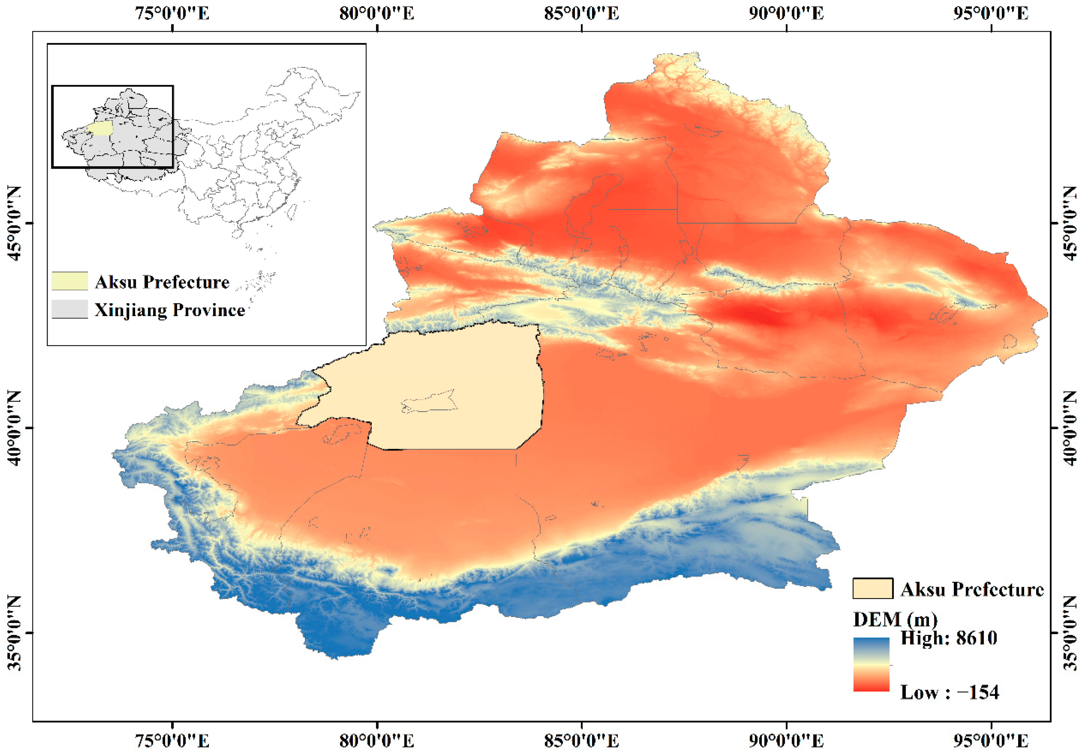
Figure 1. Location of the study area.
Remotesensing 17 03222 g001
Figure 2. Distribution of sampling points.
Remotesensing 17 03222 g002
Figure 3. Downscaling accuracy of different models. (a) CatBoost, July; (b) Random Forest, July; (c) XGBoost, October; (d) Stacking, October.
Remotesensing 17 03222 g003
Figure 4. Overall process diagram. (a) Data Collection. (b) Downscaled Stacking-SIF. (c) EC model establishment.
Remotesensing 17 03222 g004
Figure 5. Spatial distribution in July 2023: (a) GOSIF data (0.05°); (b) downscaled 0.005° SIF; (c) downscaled 30 m SIF; and (d) GPP.
Remotesensing 17 03222 g005
Figure 6. Comparison of SIF at different spatial resolutions in the Aksu region in July 2023: (a) original GOSIF image and (b) downscaled 30 m SIF image.
Remotesensing 17 03222 g006
Figure 7. Correlation analysis between SIF and soil salinity in the Aksu region: (ac) correlation in July 2023 and (df) correlation in October 2023.
Remotesensing 17 03222 g007
Figure 8. Linear Regression of Soil EC against SIF for July 2023.
Remotesensing 17 03222 g008
Figure 9. SIF estimation of soil EC results for July 2023.
Remotesensing 17 03222 g009
Figure 10. Accuracy of the SIF–EC model at different depths: (a) July 2023 and (b) October 2023.
Remotesensing 17 03222 g010
Figure 11. Soil EC distribution maps for July and October 2023. (af) EC distribution map for July. (gl) EC distribution map for October.
Remotesensing 17 03222 g011
Figure 12. Correlation analysis between SIF and GPP. (a,b) July 2023. (c,d) October 2023.
Remotesensing 17 03222 g012
Figure 13. Correlation analysis between downscaled SIF and GOSIF for July and October 2023. (a) July 2023. (b) October 2023.
Remotesensing 17 03222 g013
Figure 14. Soil EC classification results for July and October 2023. (af) July. (gl) October.
Remotesensing 17 03222 g014aRemotesensing 17 03222 g014b
Table 1. Environmental covariates.
DatasetFeaturesFormulation/Simple DescriptionReference
MODISNDMI N D M I = ( N I R S W I R ) ( N I R + S W I R ) [18]
ENDVI E N D V I = ( N I R + G ) ( 2 × R ) ( N I R + G ) + ( 2 × R ) [19]
EVI E V I = 2.5 × ( N I R R ) ( N I R + 6 R 7.5 B + 1 ) [20]
NDVI N D V I = ( N I R R ) ( N I R + R ) [21]
SIWSI S I W S I = N I R S W I R 2 N I R + S W I R 2 [22]
VSW1 V S W 1 = N I R S W I R 1 N I R + S W I R 1 [23]
VSW2 V S W 2 = N I R S W I R 2 N I R + S W I R 2 [24]
S1 S 1 = B l u e R e d [25]
SI S I = R e d + B l u e [26]
SI1 S I 1 = G × R [27]
SI2 S I 2 = G 2 + R 2 + N I R 2 [27]
SI3 S I 3 = R 2 + G 2 [28]
PLEPotential Evapotranspiration[29]
LSTLand Surface Temperature[30]
ETEvapotranspiration[31]
ETAActual Evapotranspiration[32]
LPETPotential Evapotranspiration[33]
CBNCarbon Balance Index[34]
DDIDrought Detection Index[35]
TerraClimatePRPrecipitation[36]
PETPotential Evapotranspiration[33]
DEFClimatic Water Deficit[37]
SoilGridsDTBDepth to Bedrock[38]
DTBST1Soil temperature level 1[39]
ST2Soil temperature level 2[39]
ST3Soil temperature level 3[39]
ASTER GDEMDEMDigital Elevation Model[40]
TPITopographic Position Index[41]
TWITopographic Wetness Index[42]
Table 2. Environmental covariates at different depths.
Depth2023, 72023, 10
Variable 1Variable 2Variable 1Variable 2
0–10 cmNDMIST1EVIVSW1
10–20 cmSI3DEMNDVICBN
20–40 cmSI3PRETEVISI
40–60 cmST1DEMEVIS1
60–80 cmNDMIVSW1EVIS1
80–100 cmNDMIST1AETNDVI
Table 3. Soil salinization classification.
Degree of SalinityEC (dSm−1)
Non-salinized<2
Slightly salinized2~4
Moderately salinized4~8
Severely salinized8~16
Extremely severely salinized>16
Disclaimer/Publisher’s Note: The statements, opinions and data contained in all publications are solely those of the individual author(s) and contributor(s) and not of MDPI and/or the editor(s). MDPI and/or the editor(s) disclaim responsibility for any injury to people or property resulting from any ideas, methods, instructions or products referred to in the content.