Article

Two-Step Forward Modeling for GPR Data of Metal Pipes Based on Image Translation and Style Transfer

School of Electronic Information and Electrical Engineering, Shanghai Jiao Tong University, Shanghai 200240, China
*
Author to whom correspondence should be addressed.
Remote Sens. 2025, 17(18), 3215; https://doi.org/10.3390/rs17183215
Submission received: 17 July 2025 / Revised: 9 September 2025 / Accepted: 15 September 2025 / Published: 17 September 2025

Abstract

Highlights

What are the main findings?
  • The two-step strategy, combining image translation and style transfer, achieves accurate Ground-penetrating radar (GPR) data simulation. Image translation generates precise simulated clutter-free images, and style transfer converts them to match real-world heterogeneous medium characteristics.
  • Compared to finite-difference time-domain (FDTD), the proposed method drastically reduces time costs while maintaining good performance.
What is the implication of the main finding?
  • It offers an efficient and reliable solution for GPR data simulation and analysis, sup-porting applications in geophysics, civil engineering, and other fields.
  • It enables rapid generation of high-quality GPR data, facilitating deep learning tasks like target recognition that require large labeled datasets.

Abstract

Ground-penetrating radar (GPR) is an important geophysical technique in subsurface detection. However, traditional numerical simulation methods such as finite-difference time-domain (FDTD) face challenges in accurately simulating complex heterogeneous mediums in real-world scenarios due to the difficulty of obtaining precise medium distribution information and high computational costs. Meanwhile, deep learning methods require excessive prior information, which limits their application. To address these issues, this paper proposes a novel two-step forward modeling strategy for GPR data of metal pipes. The first step employs the proposed Polarization Self-Attention Image Translation network (PSA-ITnet) for image translation, which is inspired by the process where a neural network model “understands” image content and “rewrites” it according to specified rules. It converts scene layout images (cross-sectional schematics depicting geometric details such as the size and spatial distribution of underground buried metal pipes and their surrounding medium) into simulated clutter-free GPR B-scan images. By integrating the polarized self-attention (PSA) mechanism into the Unet generator, PSA-ITnet can capture long-range dependencies, enhancing its understanding of the longitudinal time-delay property in GPR B-scan images. which is crucial for accurately generating hyperbolic signatures of metal pipes in simulated data. The second step uses the Polarization Self-Attention Style Transfer network (PSA-STnet) for style transfer, which transforms the simulated clutter-free images into data matching the distribution and characteristics of a real-world underground heterogeneous medium under unsupervised conditions while retaining target information. This step bridges the gap between ideal simulations and actual GPR data. Simulation experiments confirm that PSA-ITnet outperforms traditional methods in image translation, and PSA-STnet shows superiority in style transfer. Real-world experiments in a complex bridge support structure scenario further verify the method’s practicability and robustness. Compared to FDTD, the proposed strategy is capable of generating GPR data matching real-world subsurface heterogeneous medium distributions from scene layout models, significantly reducing time costs and providing an efficient solution for GPR data simulation and analysis.

1. Introduction

Ground-penetrating radar (GPR) has emerged as an essential geophysical technique with wide-ranging applications in numerous disciplines. In geophysics [1,2], it aids in mapping subsurface geological structures, such as identifying sedimentary layers, fractures, and voids within the earth. In civil engineering [3,4,5], GPR plays a vital role in infrastructure inspection, including detecting defects in roads, bridges, and tunnels, as well as locating underground utilities like pipes and cables. Moreover, in archaeology [6,7], it has been instrumental in uncovering buried historical artifacts and ancient structures without the need for extensive excavation. Additionally, in the military field [8,9], GPR is used for detecting hidden underground bunkers, tunnels, and caches of weapons or explosives. It can also assist in mapping the terrain beneath the surface, providing valuable information for military operations such as troop movements and strategic positioning. This helps military forces to better understand the battlefield environment and potential threats that may be concealed underground. Nevertheless, the heterogeneous nature of geological structures poses a formidable challenge. For instance, concrete, with its varying dielectric constants in different constituent phases, engenders additional electromagnetic wave scattering in the subsurface background medium. This phenomenon significantly complicates the accurate representation of complex subsurface geometries in GPR images and hampers the precise interpretation of GPR data.
To surmount these obstacles, forward modeling [10,11,12] has emerged as a prevalent simulation approach for validating the subsurface structures inferred from GPR data. Such simulations not only contribute to a profound understanding of the interaction between electromagnetic waves and the subsurface medium and the influence of measurement parameters on GPR performance but also enable the evaluation and comparison of processing and imaging methods in different detection scenarios. Compared to constructing physical tests, this approach is more efficient and cost-effective. In the field of electromagnetic wave simulation, multiple numerical techniques coexist, including the finite-difference time-domain (FDTD) method [13], the finite element method (FEM) [14], the discrete element method (DEM) [15], the pseudo-spectral time-domain (PSTD) [16] method, and the spectral element method (SEM) [17]. Among them, the FDTD method is widely utilized in GPR simulations due to its relatively easy implementation. The principle of the FDTD method involves discretizing the computational space into numerous small grid cells and also discretizing the time dimension. By approximating Maxwell’s equations using finite differences at these discrete space–time grid points, the propagation process of electromagnetic waves in the medium is simulated step by step. In each time step, the electric and magnetic field components of each grid cell need to be updated based on the field values of adjacent cells. However, it is precisely this fine grid-based calculation method that results in high time costs. When the simulation area is large and the grid division is relatively fine, the number of grid cells requiring calculation increases dramatically. Moreover, with the increase in the complexity of the subsurface medium, in order to accurately simulate the propagation of electromagnetic waves, it is often necessary to further refine the grid or increase the simulation time step, which undoubtedly further aggravates the burden of time costs and makes the FDTD less efficient in handling the simulation of complex subsurface structures.
On the other hand, deep learning (DL) techniques are making remarkable achievements in the field of GPR [18,19]. DL methods for GPR necessitate supervised learning with ground truth data, which is often arduous and costly to procure. In terms of target recognition, in 2019, N. Kim [20] proposed a DL-based underground object classification technique in processing three-dimensional (3D) GPR data. When applied to the 3D GPR data obtained from the road pavements in Seoul, South Korea, this method has achieved a 74–83% improvement in the recognition rate of cavities and a 76–93% improvement in the recognition rate of pipes compared with the traditional B-scan-based methods. However, 3D GPR technology still has several key limitations. Firstly, its data acquisition process is relatively time-consuming and labor-intensive, requiring dense and overlapping scanning lines to construct three-dimensional datasets, which increases fieldwork costs and limits its efficiency in large-area surveys. Secondly, the large volume of 3D GPR data poses high demands on computational resources for processing, stitching, and interpreting, making it challenging for applications with limited hardware conditions. In 2022, Q. Dai [21] put forward a two-stage deep neural network (DNN) named DMRF-UNet, which was designed to reconstruct the dielectric constant distribution of underground objects from GPR B-scans under heterogeneous soil conditions. This method introduced an end-to-end training approach that combined two loss functions, achieving high-precision reconstruction of the dielectric constant, shape, size, and position of underground objects. In 2024, X. Wang [22] proposed Fusion Inversion Pix2PixGAN for GPR data inversion. This method is an inversion network that integrates the reverse time migration (RTM) [23] imaging results with GPR data, enabling precise model predictions by using the fused data. Regarding the enhancement of image quality, in 2022, Z. Ni [24] introduced Declutter-GAN for generating clutter-free target images. The proposed method maps the cluttered GPR B-scan data to the clutter-free B-scan data in the training set. Compared with the subspace method, the sparse representation-based method, and the low-rank and sparse matrix decomposition (LRSD) method, Declutter-GAN exhibits higher performance in terms of computational complexity, clutter suppression results, and applicability. In 2024, Y.E. Kayacan proposed DC-ViTs [25] to remove clutter from GPR images, demonstrating the significant advantage of vision transformers (ViTs) [26] in capturing long-range dependencies and eliminating extensive clutter effects. However, these methods for GPR necessitate supervised learning with ground truth data, which is often arduous and costly to procure. The lack of accurate prior information on heterogeneous medium not only restricts the forward modeling of numerical simulation techniques but also limits the application of DL methods that rely on prior information. This results in DL methods being mostly used in target recognition and detection where the distribution of the medium does not need to be considered, while being rarely applied in forward modeling which requires taking the distribution of the medium into account.
In general, the existing methods for forward modeling of GPR have two key limitations that hinder their practicality: numerical simulation methods (such as FDTD and FEM), although widely used, are costly due to calculations based on fine grids and struggle to accurately model complex heterogeneous underground media; DL methods, on the other hand, mainly focus on tasks like target recognition or image quality improvement, relying heavily on a large amount of labeled real data. However, acquiring such data is costly and time-consuming and often impractical for heterogeneous underground environments.
In order to address the issues, this paper aims to study a two-step forward modeling strategy that integrates image translation and style transfer, which can generate realistic GPR data for complex heterogeneous underground environments without relying on annotated datasets or fine modeling of heterogeneous underground media.
  • Propose a two-step forward modeling strategy based on image translation and style transfer, enabling GPR data simulation without relying on extensive labeled data or expensive numerical calculations.
  • Develop a Polarized Self-Attention Image Translation network (PSA-ITnet) to convert scene layout images (geometric schematics of metal pipes and surrounding media) into simulated clutter-free GPR B-scan images, capturing critical longitudinal time-delay properties.
  • Design a Polarized Self-Attention Style Transfer network (PSA-STnet) to transform simulated clutter-free images into data matching the distribution of real-world heterogeneous media, preserving target information under unsupervised conditions.
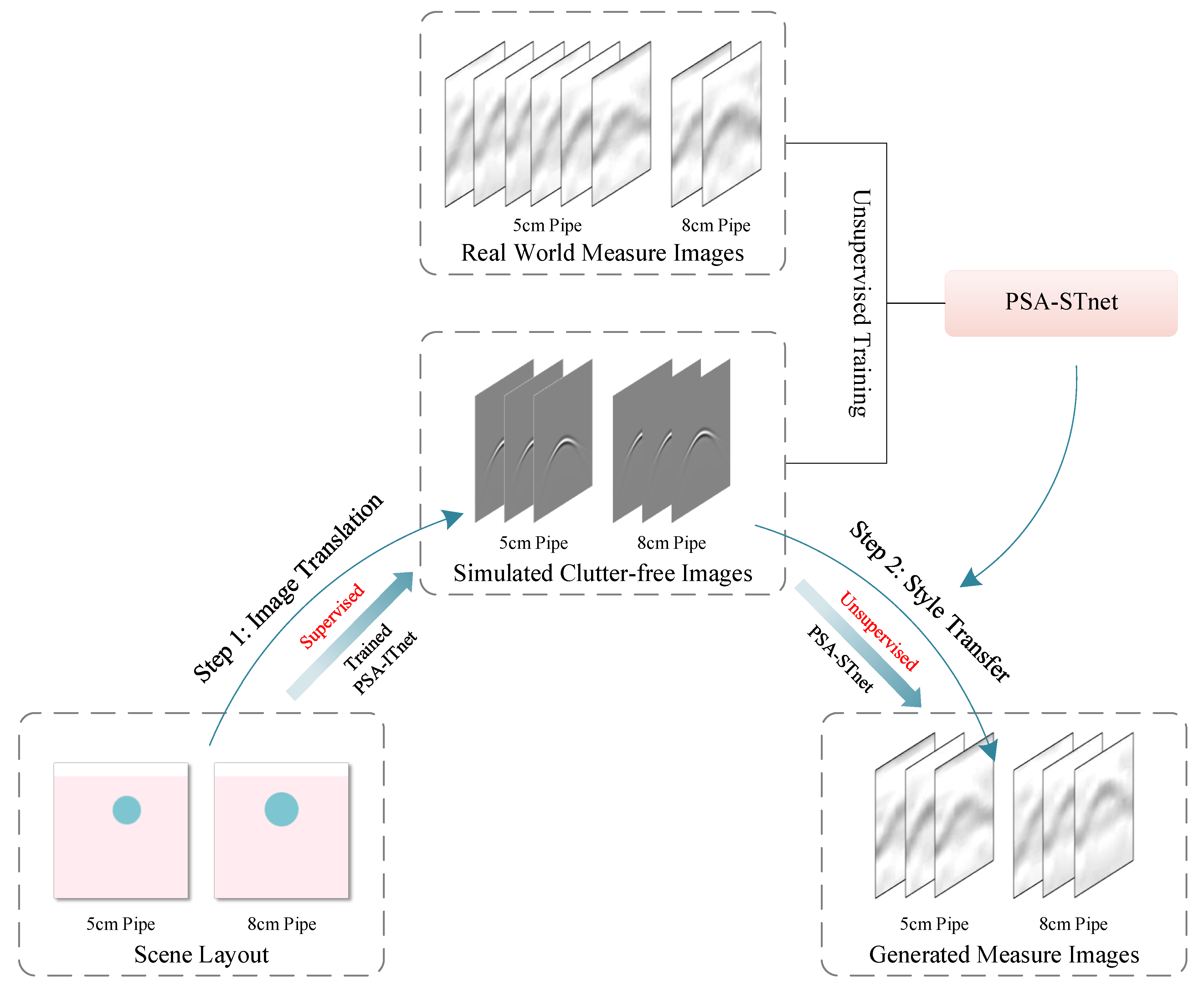
As shown in Figure 1, in Step 1, the task of image translation is carried out. Image translation refers to a technique where a model learns to convert one type of image (e.g., a schematic diagram) into another (e.g., a GPR simulation) while preserving key semantic information, enabling the transformation of abstract geometric descriptions into structured GPR responses. In Step 2, the task of unsupervised style transfer is performed. Style transfer focuses on adjusting the “style” of an image (such as clutter patterns or medium characteristics) to match a target domain (e.g., real-world GPR data) while retaining core content (e.g., target signatures), bridging the gap between ideal simulations and real-world GPR data. The strategy establishes a mapping relationship from a scene layout images to real-world GPR data. With only a few real-world GPR image samples as the target domain, it is possible to generate measured GPR data using the scene layout images. In this paper, the scene layout images in this figure are preset schematics of underground metal pipes and their surrounding media. The cross-sectional parameters (e.g., diameter, spatial location) of the metal pipes are hypothetically defined to simulate typical burial scenarios, providing controlled inputs for method validation.

2. Methods

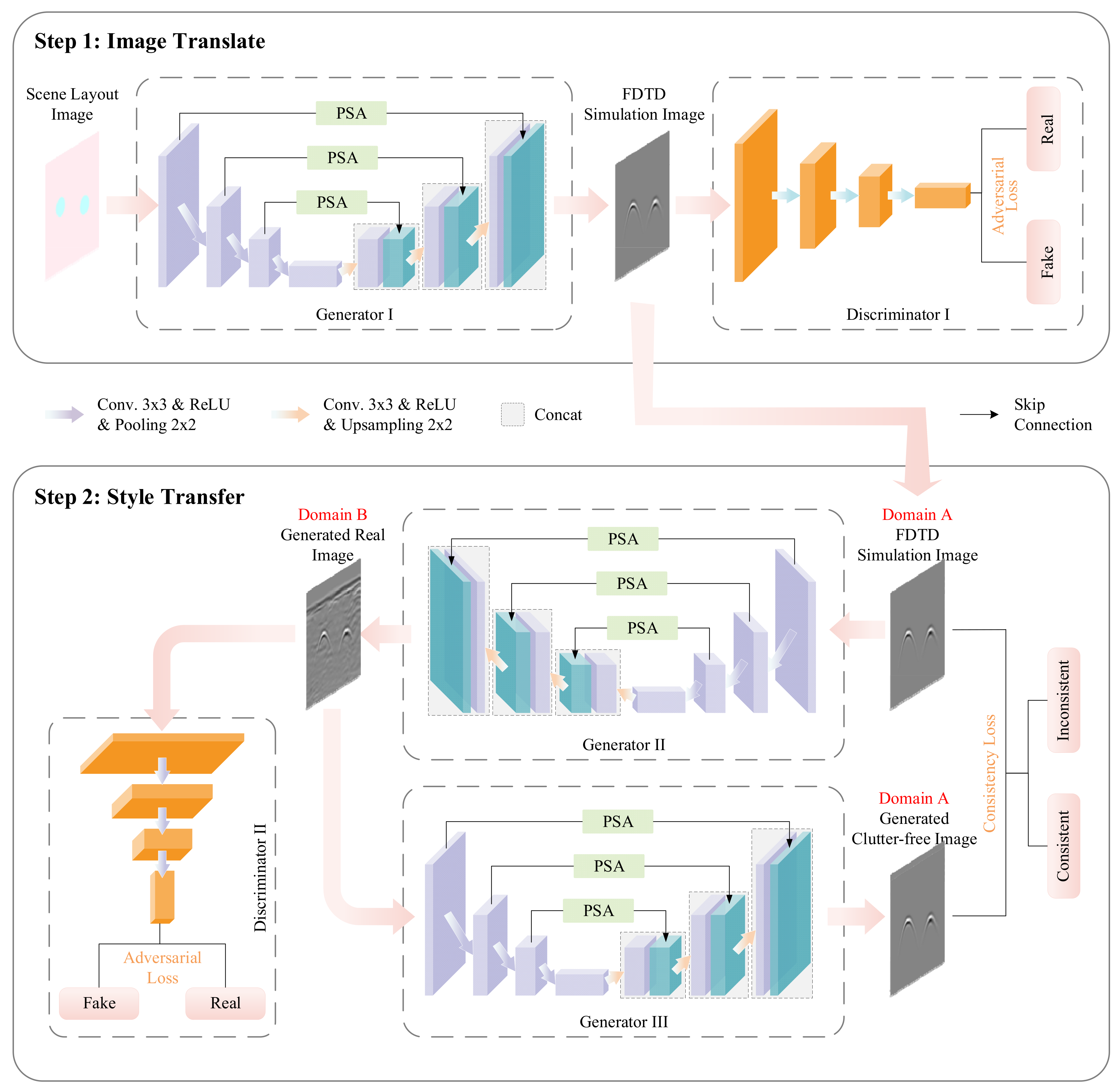
In the absence of real subsurface information, utilizing DL techniques to directly simulate GPR B-scan images from a scene layout of pipes is a complex challenge. To address this, the proposed strategy employs a two-step process that exclusively utilizes neural networks to achieve the simulation of GPR B-scan images from a scene layout of pipes. This method consists of two main components: firstly, performing an image translation task using PSA-ITnet to convert the scene layout diagrams into B-scan simulation images. Subsequently, it executes a style transfer task with PSA-STnet to transform the B-scan simulated images into generated measured images. The complete model structure is shown in Figure 2.

2.1. Step 1: Image Translation

The image translation task [27] is carried out by the PSA-ITnet proposed in this paper. Unet is the fundamental model for the proposed methods. Unet is a convolutional neural network (CNN) architecture specifically designed for image tasks. Originally proposed by O. Ronneberger [28] in 2015, Unet has gained significant popularity in various fields, including biomedical image processing, remote sensing, and GPR data analysis. Its architecture effectively captures both spatial and contextual information, making it particularly suitable for tasks where precise localization is essential.

2.1.1. PSA-ITnet Structure

The PSA-ITnet has two main components: a generator and a discriminator. The generator includes an encoder, a decoder, and the skip connections replaced by polarized self-attention (PSA). The discriminator consists of the encoder within the generator.
The encoder portion is composed of a series of convolutional layers followed by pooling layers, which progressively downsample the input image while extracting features. This process can be mathematically represented as (1) and (2).
X l = F a W l W l 1 + b l
F a ( x ) = max ( 0 , x )
where F a is the activation function, W l represents the convolutional kernels of the l -th layer, X l represents the feature map of the l -th layer, b l denotes the biases, and denotes the convolution operation.
The decoder part employs upsampling operations followed by convolutions to gradually restore the spatial dimensions of the feature maps as (3).
Y l = F a W l U p S a m p l i n g X l + b l
where U p S a m p l i n g refers to the upsampling operation and W l and b l are the weights and biases of the convolutional layers in the decoder.
Skip Connections (PSA): A distinctive feature of Unet is the inclusion of skip connections, which link the feature maps from the encoder to the corresponding layers in the decoder. These connections help retain spatial information that might be lost during downsampling, allowing the model to produce more accurate segmentations.

2.1.2. Polarized Self-Attention Mechanism

The generator’s learning process is essentially a weighted sum of features along two dimensions. Firstly, a weighted sum along the channel dimension is for estimating the output of different classes. Secondly, a weighted sum along the spatial dimension is for detecting pixels with the same semantics. To highlight these two characteristics of the PSA-ITnet, an attention mechanism is implanted in the skip connection in this paper. Suppose a self-attention module A ( · ) takes X as input and generates Z as output, where X R e C i n × H × W and Z R e C o u t × H × W . For a set of feature tensors extracted by a CNN, the full-tensor self-attention mechanism is dedicated to highlighting its element dimension features as (4).
Z = A X X
where ⊙ is a multiplication operator. X represents the feature map, A ( · ) represents the self-attention module, and Z represents the output result of the self-attention module. However, this kind of attention mechanism is extremely complex and susceptible to noise, making it difficult to learn directly.
To address these challenges, this paper draws on PSA [29] and performs polarization filtering in attention calculation. The self-attention module is analogized to the polarization filtering of an optical lens, aiming to highlight features in specific directions, which is similar to only allowing light in specific directions to pass through. But it may lead to a reduction in overall intensity and further enhancement is needed to achieve better results, which is similar to the process of polarization filtering and subsequent enhancement in photography. A self-attention module acts on the input tensor X to highlight or suppress features, much like an optical lens filtering light. In photography, there are always random rays in the transverse direction that can cause glare or reflection. Polarization filtering only permits light perpendicular to the transverse direction to pass through, which has the potential to increase the contrast of photos. Due to the loss of total intensity, the filtered light usually has a smaller dynamic range and thus requires additional enhancement, such as through high dynamic range enhancement.
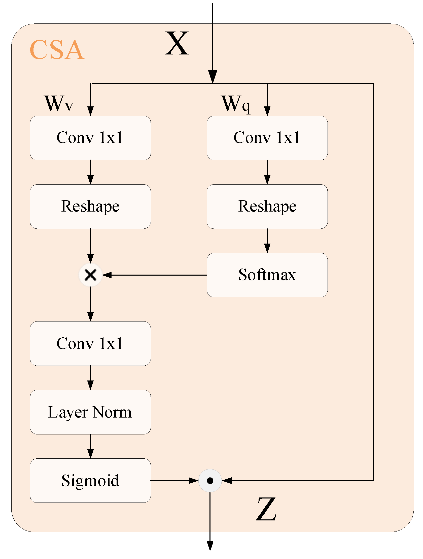
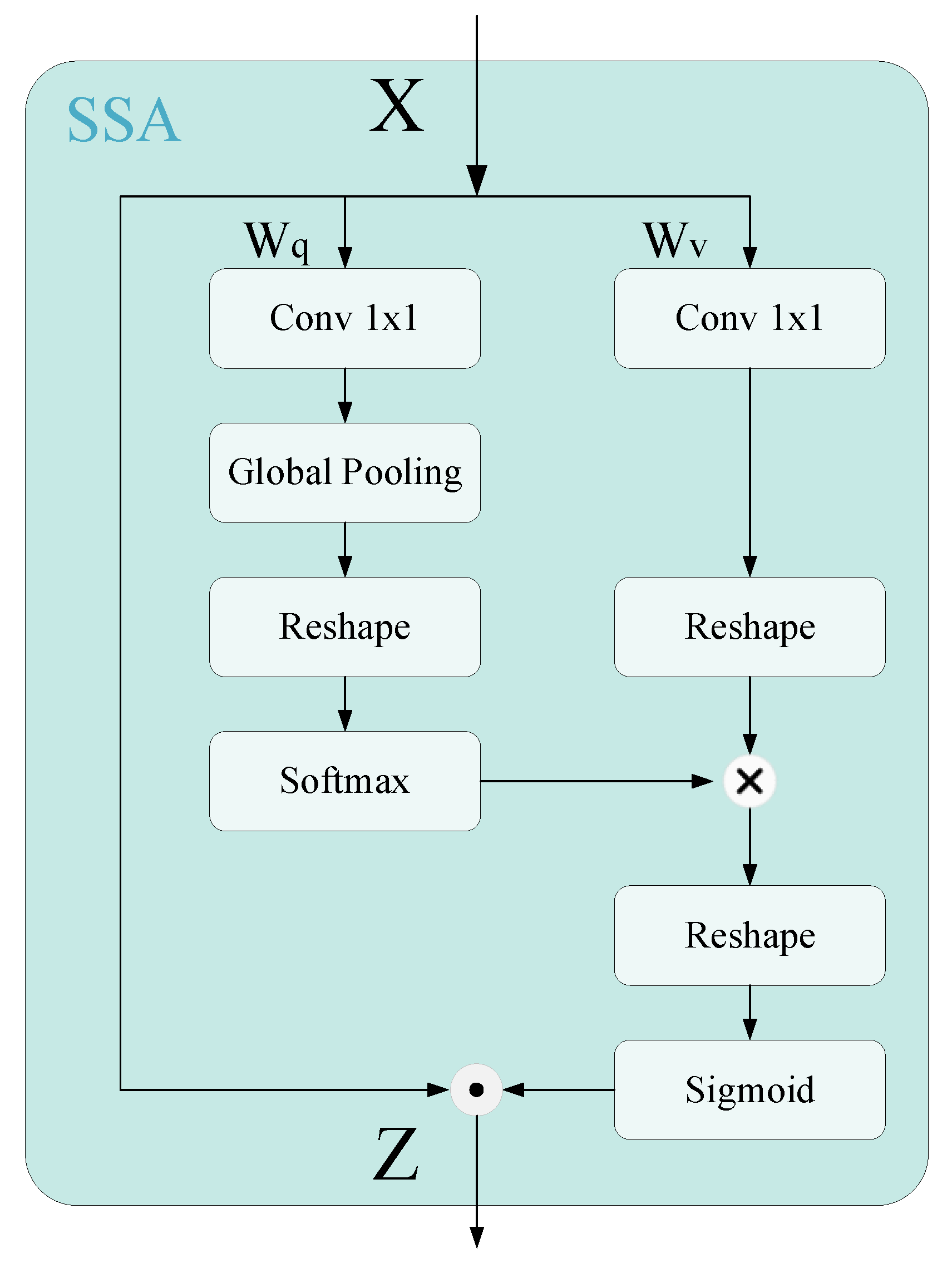
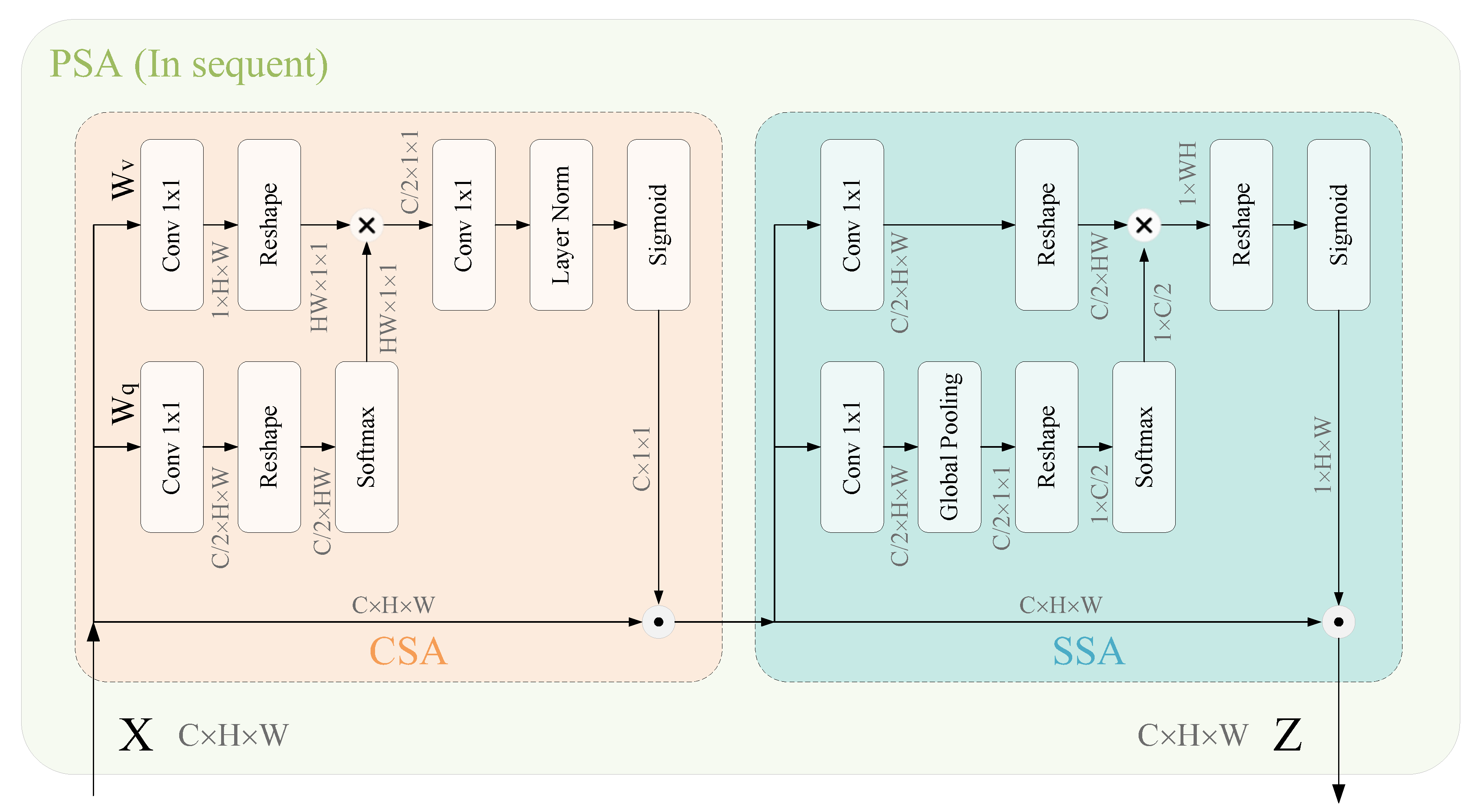
The self-attention module operates on the input tensor, similar to the polarization filtering of an optical lens, which can highlight or suppress features. However, this may lead to a reduction in the dynamic range of features. Therefore, a method similar to high dynamic range enhancement is needed to restore and enhance the details of features. Specifically, the PSA mechanism can be instantiated as two branches, channel self-attention (CSA) and spatial self-attention (SSA), corresponding to Figure 3 and Figure 4, respectively.
  • Channel self-attention branch
Figure 3. Illustration of Channel Self-Attention.
Remotesensing 17 03215 g003
The CSA flow chart is shown in Figure 3. Specifically, CSA is defined as A c h X R e C × 1 × 1 , which can be formulated as (5).
A c h X = F S G W z R 1 W v X × F S M R 2 W q X
where A c h · is channel self-attention mechanism. W v , W q , and W z are 1 × 1 convolutional layers, respectively. × is the matrix dot-product operation. R 1 and R 2 are two tensor reshaping operators. F S M · is the SoftMax operator, that is (6). And F S G · is the sigmoid operator, that is (7).
F S M X = j = 1 N p e x j m = 1 N p e x m x j
F S G X = 1 1 + e X
where x j and x m represent the j -th and m -th elements of the input vector X , respectively, and N p represents the dimension of the input vector. The internal channel number between W v , W q , and W z is C / 2 . The output of the CSA is (8).
Z c h = A c h X c h X R e C × H × W
where c h is the channel multiplication operator. Z c h represents the output processed by the channel self-attention mechanism.
  • Spatial self-attention branch
The SSA flow chart is shown in Figure 4. Specifically, SSA is defined as A s p X R e 1 × H × W , which can be expressed as (9).
Figure 4. Illustration of Spatial Self-Attention.
Remotesensing 17 03215 g004
A s p X = F S G R 3 F S M R 1 F G P W q X × R 2 W v X
where A s p · is spatial self-attention mechanism. For the input X , W q and W v are obtained through standard 1 × 1 convolution layers, respectively. R 3 is a tensor reshaping operator. F G P · is a global pooling operation on W q X , that is (10).
F G P X = 1 H × W i = 1 H j = 1 W X : ,   i ,   j
where H and W represent the height and width dimensions of the input, respectively. The values at all spatial positions of each channel are summed and averaged. R 1 , R 2 , and R 3 are three tensor reshaping operators. F S M · is the SoftMax function. × is the matrix dot product operation. Then, the output of the spatial-only branch is (11).
Z s p = A s p X s p X R e C × H × W
where s p is a spatial-wise multiplication operator. Z s p represents the output processed by the channel self-attention mechanism.
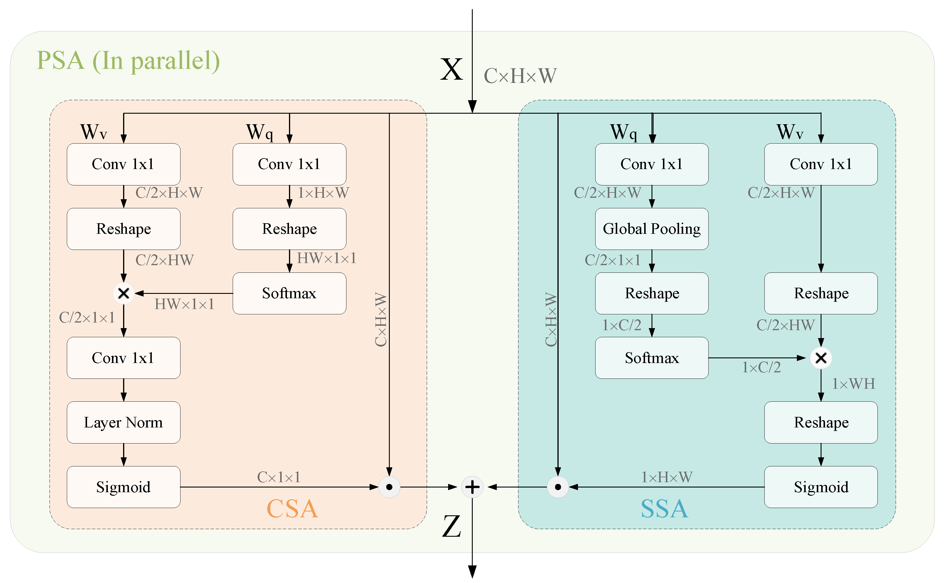
As shown in Figure 5, the outputs of the above two branches can be composed under the parallel layout as (12).
P S A p X = A c h X c h X + A s p X s p X
where P S A p · is polarized self-attention mechanism in parallel. In parallel, the output Z c h of the channel branch and the output Z s p of the spatial branch are combined through element-wise addition.
Or the outputs can be composed under the sequential layout as (13).
P S A s X = A s p A c h X c h X s p A c h X c h X
where P S A s · is polarized self-attention mechanism in sequence. As shown in Figure 6, in sequence, first, the output of the channel branch A c h X c h X is applied with the operation of the spatial branch A s p A c h X c h X . Then, it is combined with A c h X c h X through element-wise multiplication operation s p to obtain the final combined output   P S A s X under the sequential layout.

2.2. Step 2: Style Transfer

Due to the difficulty in knowing the distribution and properties of an underground heterogeneous medium, it is not feasible for FDTD to accurately model a heterogeneous medium and thus cannot simulate complex real-world scenarios. There exists a hard-to-bridge gap between simulation images and measured GPR images with a mess of clutter. To cross this gap, based on the principle of cycle consistency, this paper uses a style transfer model to convert simulation images into images with a similar distribution to real GPR images, thereby realizing a complete forward modeling process.
This paper proposes the PSA-STnet to execute the style transfer task [30]. The PSA-STnet is predicated on the principle of cycle consistency [31], which serves as a fundamental tenet for ensuring the model’s stability and efficacy. Cycle consistency, in essence, mandates that, when an input image undergoes a transformation from Domain A to Domain B and subsequently back to Domain A, the model should endeavor to maintain the highest possible degree of similarity to the original image. This similarity is quantitatively assessed by comparing the disparities between the original image and the image obtained after the round-trip transformation. The architecture of PSA-STnet, as depicted in Figure 2, is composed of two generators with isomorphic structures and a solitary discriminator. The generators are founded upon the PSA-ITnet architecture. The discriminator in style transfer also is constructed using the encoding part of the generator. During the training process, the model is steered by two types of losses: adversarial loss and consistency loss. Domain A is defined as the simulated clutter-free dataset, while Domain B is defined as the measured GPR dataset with a mess of clutter. The training process unfolds in the following manner: Generator II ( G I I ) takes the simulated clutter-free images from Domain A as input and aims to transmute them into raw measured GPR images with a mess of clutter in Domain B. The adversarial loss in the discriminator then assesses whether the converted images possess the characteristics of Domain B. Subsequently, the generated images are passed through Generator III ( G I I I ) to be converted back from Domain B to Domain A. Finally, the consistency loss determines whether the image obtained after this reverse transformation is congruent with the simulated clutter-free image. Through this iterative process, the model progressively learns to adaptively transform the simulated clutter-free images into the raw GPR data with mass, rife with clutter, thereby attaining the GPR data that conforms to the distribution and properties of the underground heterogeneous medium.
During the training process, the model is guided by two types of losses: adversarial loss and consistency loss:

2.2.1. Adversarial Loss

Adversarial loss is mainly used in generative adversarial networks (GANs). In a GAN [32], there are a generator and a discriminator. The generator aims to generate samples that are as realistic as possible to deceive the discriminator, while the discriminator aims to distinguish between real samples and those generated by the generator. For the discriminator, if the real data distribution is P d a t a x and the data distribution generated by the generator is P G x , then the goal of the discriminator D is to maximize the probability of correctly distinguishing real samples from generated samples, which can be expressed as (14).
V D , G = E x p d a t a x log D x + E z p z z log 1 D G z
where x is a sample from the real data distribution, z is noise input from a prior distribution, and G ( z ) is the sample generated by the generator according to noise z . For the generator, its goal is to minimize the adversarial loss so that the generated samples can deceive the discriminator, that is, making the discriminator think the generated samples are real.
The adversarial loss of the generator can be expressed as (15).
m i n   G m a x D V D , G = E x p d a t a x log D x + E z p z z [ l o g ( 1 D ( G ( z ) ) ) ]
Through continuous optimization of the adversarial loss, the generator and discriminator conduct adversarial training, gradually improving the quality of generated samples and the discriminative ability of the discriminator. Eventually, the generator can generate extremely realistic samples, making it difficult for the discriminator to distinguish between real samples and generated samples. However, in style transfer, the input to G I I I is not noise but the simulation clutter-free images from Domain A. The objective of G I I I is to generate images in Domain B that closely resemble the real images in Domain B in terms of features. The discriminator D aims to accurately distinguish between the real image b from Domain B and the generated images G I I I ( a ) from Domain A. The adversarial loss function is thus expressed as (16).
L G A N G I I I ,   D ,   a , b = E b p d a t a   b log D b                                                                                                         + E a p d a t a a log 1 D G I I I a

2.2.2. Consistency Loss

The consistency loss plays a pivotal role in ensuring the fidelity and stability of the image transformation process. While the adversarial loss in the model enables the generator ( G I I ) to learn the distribution characteristics of the target domain (Domain B), it does not inherently guarantee the preservation of the original image content during the transformation from the input image ( a ) in the source domain (Domain A) to the generated image G ( a ) . This is because the adversarial loss primarily focuses on matching the distribution of the generated images to that of the target domain, without imposing explicit constraints on maintaining the semantic and structural integrity of the individual images. The essence of the consistency loss lies in its ability to enforce a form of cyclic consistency within the model’s transformation process. Specifically, it ensures that when an image is transformed from Domain A to Domain B and then back to Domain A, the resulting image should be as similar as possible to the original input image. This similarity is quantified in terms of the L 1 norm distance between the original image and the reconstructed image after the round-trip transformation.
Mathematically, the consistency loss is defined as (17).
L c o n G I I , G I I I , a , b = E a p d a t a   a G I I I G I I a a 1
where G I I represents the generator that transforms images from Domain A to Domain B and G I I I is the generator responsible for the reverse transformation from Domain B back to Domain A. The expectation E is taken over the distribution of the input images a from the data p d a t a a . The L 1 norm · 1 is used to measure the difference between the original image a and the reconstructed image G I I I ( G I I ( a ) ) on a pixel-by-pixel basis. By minimizing this consistency loss, the model is encouraged to learn a transformation that not only maps the input images to the target domain distribution but also preserves the essential characteristics and content of the original images.
The incorporation of the consistency loss into the multi-loss function of style transfer is what enables the model to strike a delicate balance between learning the distribution characteristics (through the adversarial loss) and preserving the image content (through the consistency loss). The multi-loss function is expressed as (18).
L G I I , G I I I , a , b = L G A N G I I ,   D , a , b + λ L c o n s i s t e n c y G I I , G I I I , a , b                                                                 = E b p d a t a b log D b + E a p d a t a a l o g 1 D G I I a + λ E a p d a t a a G I I I G I I a a 1
where λ serves as a hyperparameter that controls the relative importance of the consistency loss compared to the adversarial loss. By adjusting the value of λ , the model can be fine-tuned to prioritize either distribution learning or content preservation, depending on the specific requirements of the application.
This multi-loss strategy significantly improves the overall performance and reliability of the process of generating expected images in style transfer. It enables the model to generate GPR images of real subsurface medium distributions and properties. These images are not only very similar to the characteristics of the target domain but also maintain the integrity and meaningful information of the original input images.

3. Simulation Experiments

Although the FDTD method cannot accurately model the heterogeneous medium in real-world scenarios (where medium properties are often unknown or unquantifiable), it conducts fine discretization on the differential form of Maxwell’s equations and exhibits ideal simulation performance under preset, precisely defined heterogeneous medium conditions (such as sand–clay mixed soil with known dielectric constants). This reliability has made it widely recognized in the academic community [33,34,35,36]. In the simulation experiment, this paper takes the FDTD simulation results under the preset randomly mixed clay and sand medium as the benchmark to evaluate the performance of the proposed method, aiming to verify that, compared with the FDTD method, the proposed method achieves higher time efficiency with a small loss of accuracy.

3.1. Dataset Preparation

In order to make the corresponding dataset structures meet the requirements of the proposed algorithm, this study constructs three sets of image data, as shown in Figure 7, namely scene layout images, simulation clutter-free images, and simulation images with a mess of clutter under soil medium conditions. Each of these three types of images encompasses 1000 sample images. Specifically, the scene layout and clutter-free images possess a one-to-one correspondence relationship and are utilized to execute the image translation task in Step 1. In contrast, the clutter-free images and images with clutter do not have a one-to-one correspondence relationship, employed to carry out the unsupervised style transfer task in Step 2.
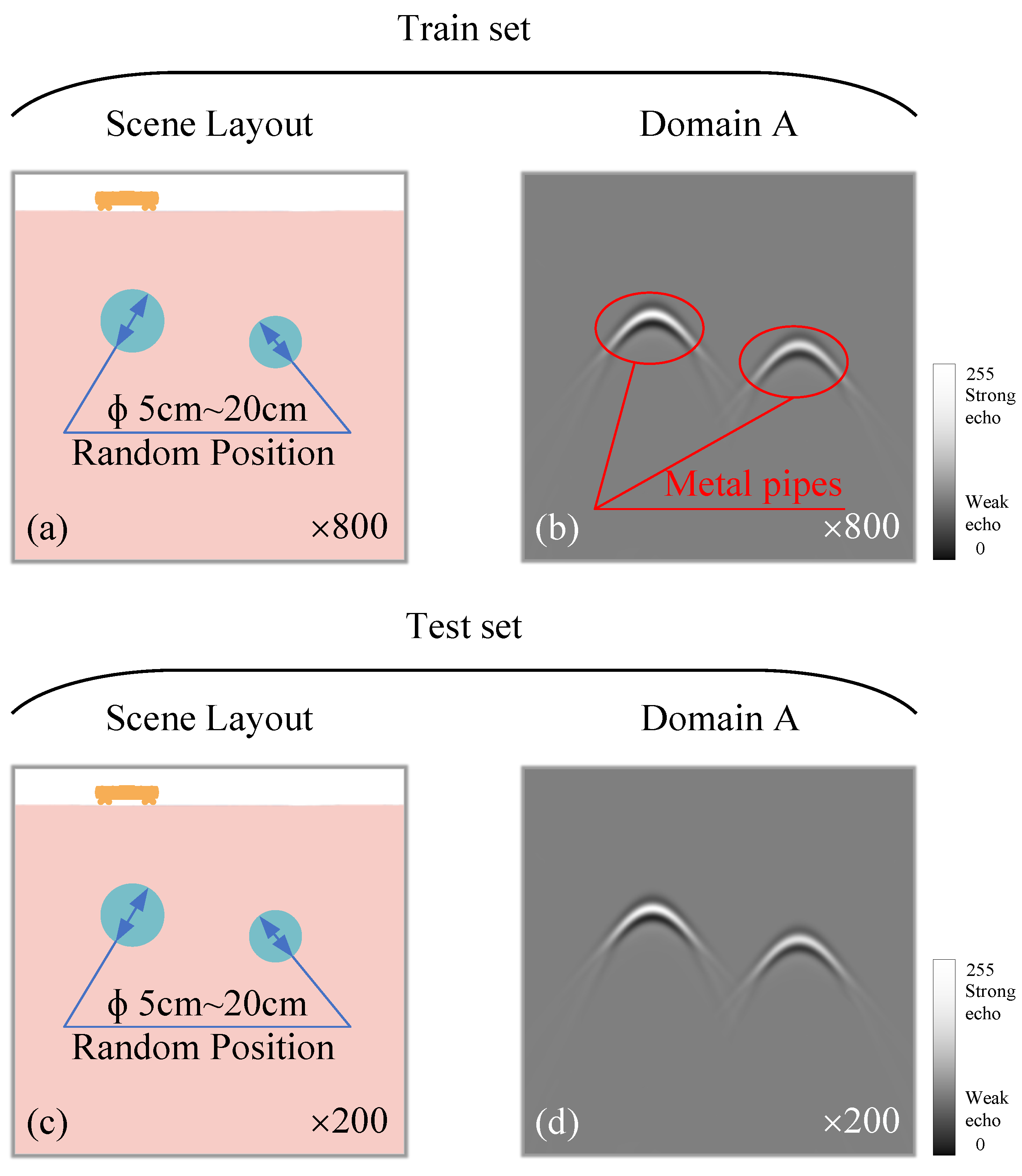
It is noteworthy that the majority of the sample images within these three types of images contain two metal pipe targets. However, in Domain B, the 400 images are designed to include only one metal pipe target, and these samples are considered as contaminated samples for the training phase. Their primary functions are to validate the training results of the network and to examine whether the proposed network undergoes overfitting after training. In the event of overfitting, the network might infer from the clutter-free images containing two metal pipe targets to the actually measured images with only one metal pipe target. The structure of the dataset for the image translation task is depicted in Figure 8. Specifically, 800 pairs of samples are employed for the training of PSA-ITnet in Step 1, while 200 pairs of samples are utilized for testing purposes. Figure 8a,c represents the simulation scenarios, and Figure 8b,d respectively correspond to the simulation images of Figure 8a,c.
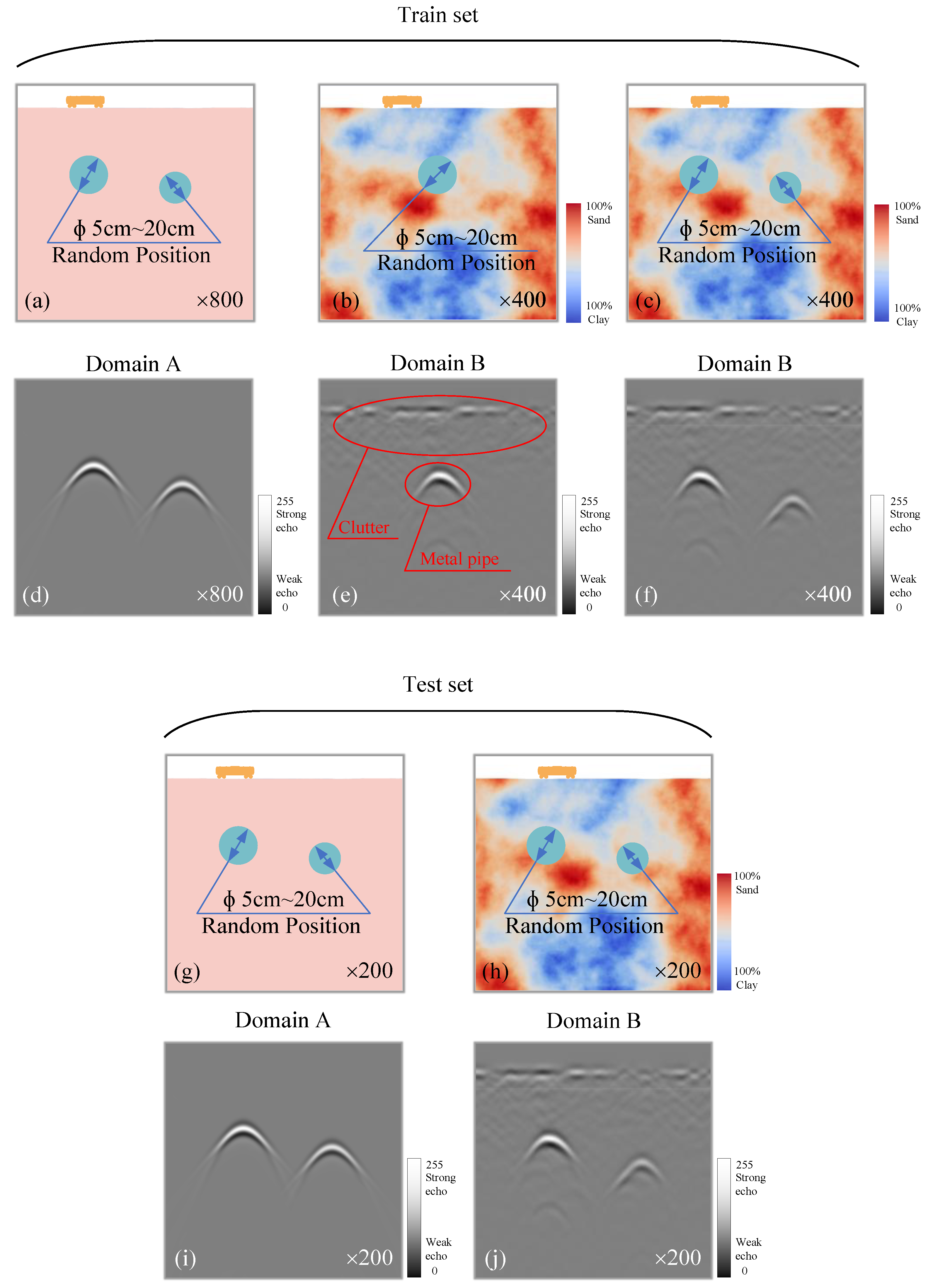
The structure of the dataset for the style transfer task is shown in Figure 9. Among them, 800 images from Domain A and 400 images each from Domain B containing either one or two metal pipe targets are used for the unsupervised style transfer task in Step 2. Additionally, 200 pairs of metal pipes with two targets are reserved for testing. It is worth noting that the 200 pairs of clutter-free images and images with clutter used for testing have a one-to-one correspondence relationship. In contrast to the unsupervised nature of the training set, the supervision information in the testing set is designed to evaluate the performance of the proposed method. As shown in Figure 9, Figure 9a–c,g,h represent the scene layout images, Figure 9a,g are the simulation clutter-free images under homogeneous medium conditions, Figure 9b,c,h are the simulation images with clutter under soil medium conditions. Figure 9d–f,i,j are the simulation results corresponding to Figure 9a–c,g and h, respectively. To avoid loss of generality, except for Figure 9e,f which correspond to the Domain B images containing one metal pipe, the rest all correspond to two metal pipes, with the diameters of these metal pipes randomly varying between 5 cm and 20 cm, and the position of the metal pipes follows a uniform random distribution within the simulation area. However, due to the focus of this research on the situation where the echoes from different targets in the same scene are relatively independent, which serves as a preliminary verification of our method, and considering that we have not yet extended it to the scenario where targets overlap with ground objects, we have imposed certain constraints on the metal pipes’ positioning. For the two metal pipes, the minimum horizontal spacing between them is set to 10 cm. This constraint is in line with the subsequently collected real-world GPR scenarios, which is beneficial for verifying the effectiveness of the proposed method. In particular, Figure 9b,c and h illustrate that the underground heterogeneous medium is soil randomly mixed with sand and clay. The size of the simulated dataset scene is 100 × 100 × 0.1 cm3. The geometric dimensions and electromagnetic parameters of each layer of medium and the metal pipe are detailed in Table 1. The discrete grid is d x = d y = d z = 0.1   c m . The simulation time for each scan is 10 ns. Additionally, to eliminate the influence of boundary reflections, the boundaries of the model are equipped with a perfect matching layer (PML) consisting of 50 grids.
The simulated GPR uses a Ricker wave with a central frequency of 1.5 GHz as the transmitting pulse. Both the transmitting and receiving antennas are positioned 5 cm above the subsurface medium. They move along one end of the scene from 5 cm to 95 cm with an increment of 0.5 cm. The input and output sizes of the model are both 256 × 256   p i x e l s , corresponding to an area of 90 × 90 × 0.1 cm3 (excluding the perfect matching layers at the scene boundaries).
Among them, the number of scene layout images and the simulation clutter-free images in Domain A are 1000, and there is a one-to-one correspondence between the two sets of images. Meanwhile, there are 500 simulation images of the heterogeneous medium with one metal pipe and 500 with two metal pipes in Domain B, respectively, and there is no one-to one correspondence with the simulation clutter-free images in Domain A.

3.2. Analysis of Image Translation Results

The property of longitudinal time delay in B-scan images is a crucial issue that needs to be addressed in image translation. The B-scan image is constructed through multiple measurements by the GPR at different positions. During the operation of GPR, the transmitting antenna emits high-frequency electromagnetic pulses into the ground, and these pulses propagate in the underground medium. When encountering interfaces between different mediums or target objects, part of the electromagnetic pulses is reflected. The receiving antenna receives these reflected wave signals, and each received signal is A-scan data.
When constructing the B-scan image, the GPR is moved along the detection path, and A-scan data are collected at multiple positions. The horizontal axis of the B-scan image usually represents the horizontal moving distance of the radar on the ground, that is, spatial position information. The vertical axis is composed of the time information in these A-scan data. Since the A-scan data at different positions are arranged on the vertical axis according to the time information of their reflected waves, and this time information is directly related to the depth of the target object, the vertical axis of the B-scan image actually reflects the target response time [37].
When electromagnetic waves propagate in underground media, since the dielectric constant of the underground medium is greater than that of air, the response time becomes longer when the relative position between the radar and the metal pipe remains unchanged [38]. In B-scan images, this is manifested as the top of the hyperbolic target being slightly lower than the top of the cross-section of the metal pipe in the scene layout.
In fact, it is quite difficult for a neural network to comprehend the time-delay characteristics of the ordinate in B-scan images. The neural network is more adept at translating objects in fixed spatial positions into other forms.
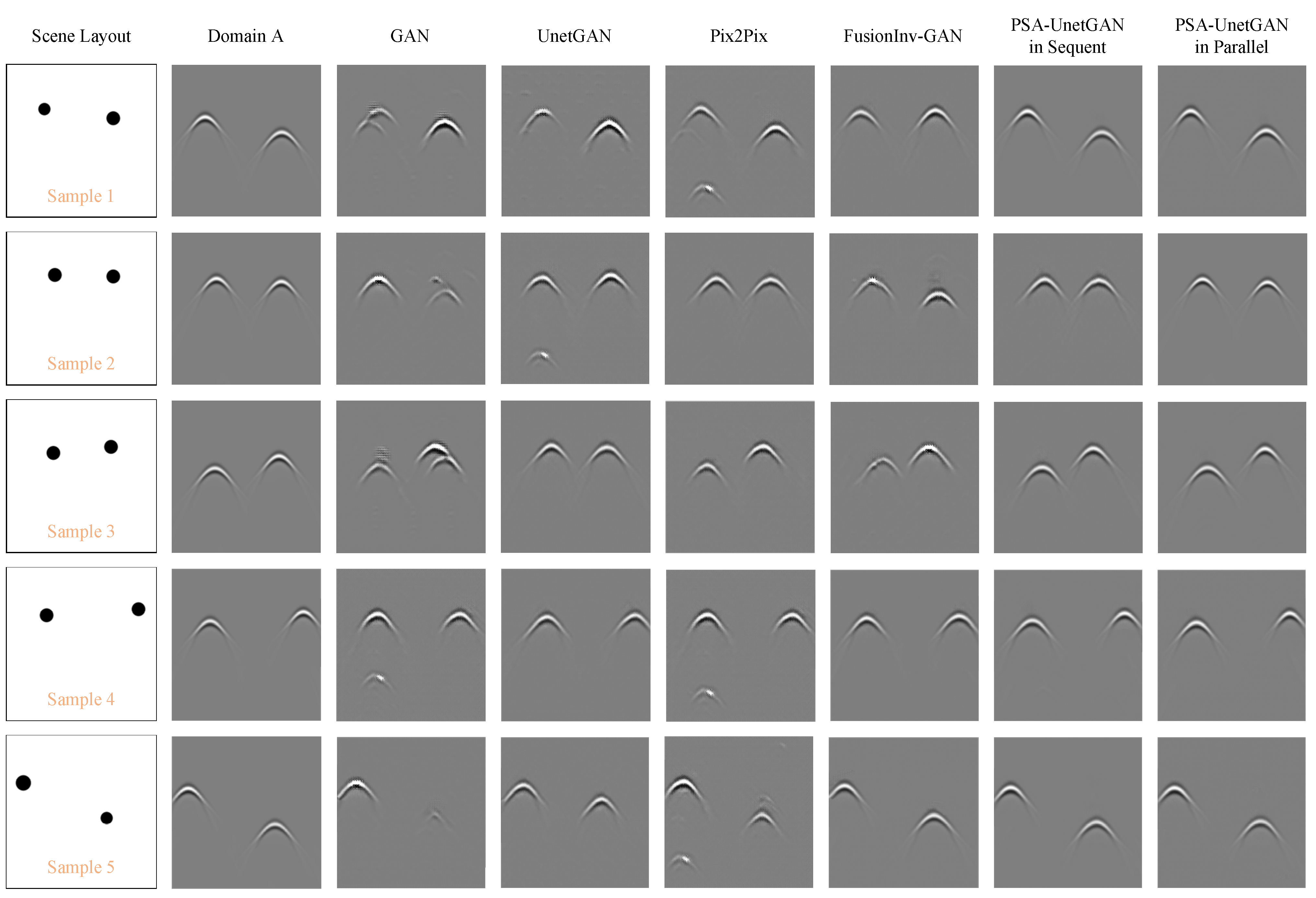
From Step 1 of the simulation experiment, five sample images of scene layouts, the corresponding simulation clutter-free images (Domain A), and the visualization experimental results of the six corresponding image translation methods are presented in Figure 10. In the images of Domain A, the two hyperbolas corresponding to the two metal pipes are slightly lower in spatial distribution than the two black circles representing the cross-sections of the metal pipes in the scene layout diagram, which is consistent with the aforementioned principle. Image translation usually conducts mapping relationships of pixel-level corresponding spatial positions and is more capable of generating a hyperbola at the location of the circles rather than at a slightly lower position. However, the physical meaning of the vertical direction in GPR B-scan images is time delay, which poses higher requirements for style transfer networks to understand deeper semantic meanings.
Among the results corresponding to the six image translation methods, the generated images of the GAN are unstable. This is because, during the image generation process of the GAN, there is uncertainty regarding the position of generating the hyperbola. From the perspective of image semantics, the GAN fails to understand whether the hyperbola should be located at the position of the black circle representing the cross-section of the metal pipes or at a slightly lower position. This hesitation reflects the GAN’s insufficient understanding of the semantic relationship between the scene layout and the target object in the image. For the metal pipe, the GAN is unable to stably generate the hyperbola structure either at the position of the black circle or at a lower position, indicating that the GAN lacks the ability to accurately map the structural features of the target object in the image. Relying solely on its existing generation mechanism, it cannot handle such complex semantic and spatial relationships.
UnetGAN, based on the Unet generator, performs better because the Unet structure endows it with certain advantages; although, like the traditional GAN, it fails to understand the complex physical property of the longitudinal time delay in the B-scan, it can generate a relatively complete hyperbola structure at the position of the black circle. This is due to the architectural characteristics of the Unet. Its encoder–decoder structure can better capture local and global information, enabling the model to generate, to a certain extent, a hyperbola structure related to the information of the cross-section of the metal pipe represented by the circle in the scene layout diagram, thereby performing better than the traditional GAN in image translation.
When translating circular cross-sections in scene layout into hyperbolas in Domain A, Pix2Pix demonstrates a superior ability to preserve the information of target hyperbolas, showcasing a more advanced understanding of the structural information of target hyperbolas compared to UnetGAN. However, it is regrettable that Pix2Pix is more prone to generating artifacts than UnetGAN.
Building on Pix2Pix, FusionInv-GAN not only preserves the information of target hyperbolas but also eliminates the influence of artifacts, demonstrating enhanced robustness in structural feature retention and artifact suppression. However, this improved model still exhibits insufficient understanding of the longitudinal time-delay characteristics inherent in GPR B-scan images. It lacks mechanisms like PSA to capture long-range dependencies in the vertical dimension, unable to interpret the vertical axis as time-delay information.
Furthermore, the PSA-ITnet can understand whether to generate the hyperbola at the position of the black circle or at a lower position. The core principle lies in polarizing the input features, analyzing them by dividing them into different channels or directions. During the image translation process, the PSA can effectively capture long-distance dependence relationships and complex semantic information, calculate the importance weights of the features at each position with respect to the features at other positions, and redistribute the feature representations according to these weights, enabling the model to focus on the key information parts in the input data. For the complex physical semantics of the longitudinal time delay in the B-scan image, the PSA helps the PSA-ITnet to better understand. It can associate the features corresponding to the time-delay information with other spatial features and integrate this physical semantics through the adjustment of the attention weights.
On the other hand, the PSA-ITnet in both sequent and parallel configurations have achieved similar visualization results, making it difficult to distinguish which one is superior. Therefore, this study utilized three full-reference evaluation metrics [39] to quantitatively assess the image translation methods: mean squared error (MSE), peak signal-to-noise ratio (PSNR), and structural similarity index (SSIM).
For an image of size M × N , with the original image I ( x , y ) and the translated image I ^ ( x , y ) , the MSE is calculated as (19).
M S E = 1 M × N x = 0 M 1 y = 0 N 1 I x , y I ^ x , y 2
A lower MSE indicates better pixel-wise accuracy. PSNR is given by (20).
P S N R = 10 l o g 10 M a x I 2 M S E
Higher PSNR values signify better image quality and signal fidelity. SSIM, which considers structural, luminance, and contrast similarities, has a form as (21).
S S I M x , y = 2 μ x μ y + C 1 2 σ x y + C 2 μ x 2 + μ y 2 + C 1 σ x 2 + σ y 2 + C 2
where μ x and μ y are the means, σ x and σ y are the standard deviations, σ x y is the covariance of the original and generated images in local regions, and C 1 , C 2 are constants to avoid division by zero. An SSIM value closer to 1 implies better visual similarity.
The quantitative evaluation results of image translation are presented in Table 2. The FDTD is used as a benchmark to evaluate the effectiveness of PSA-ITnet. For FDTD itself, MSE, PSNR, and SSIM are 0, +∞, and 1, respectively. The GAN exhibits the poorest performance in terms of the three metrics, namely MSE, PSNR, and SSIM. This is due to its insufficient understanding of the semantic relationships between the scene and the target objects during the image generation process, resulting in significant discrepancies between the generated images and the original images in terms of pixels, signals, and structures. The UnetGAN, which is based on the Unet architecture, outperforms the GAN in all three metrics. Its encoder, decoder, and skip connections enable it to better capture local and global information. However, it shows slight insufficiency in preserving hyperbolic target structures. Compared to Unet, Pix2Pix demonstrates superior capability in retaining hyperbolic target structures but tends to introduce artifact issues. FusionInv-GAN not only preserves hyperbolic target information but also avoids artifacts. However, it underperforms in handling complex physical semantics such as longitudinal time delays. The PSA-ITnet shows improvements in the three metrics compared to the FusionInv-GAN. Nevertheless, the series structure has limitations in information transmission. The MSE, PSNR, and SSIM of the PSA-ITnet (in parallel) reach 4.182, 41.917 dB, and 0.953, respectively. It demonstrates the best performance among all the methods. Its parallel structure can effectively avoid information bottlenecks, fully exploiting the advantages of the PSA. The generated clutter-free images are closest to the simulated clutter-free images in terms of pixel accuracy, signal fidelity, and structural similarity.

3.3. Analysis of Style Transfer Results

In contrast to the image translation task, the model is not required to understand the time-delay nature in the vertical direction of B-scan images. Instead, in the style transfer task, the requirement for the model is to generate measured images (Domain B) that conform to the characteristic distribution of a real-world underground heterogeneous medium without damaging the target information in simulated clutter-free images (Domain A).
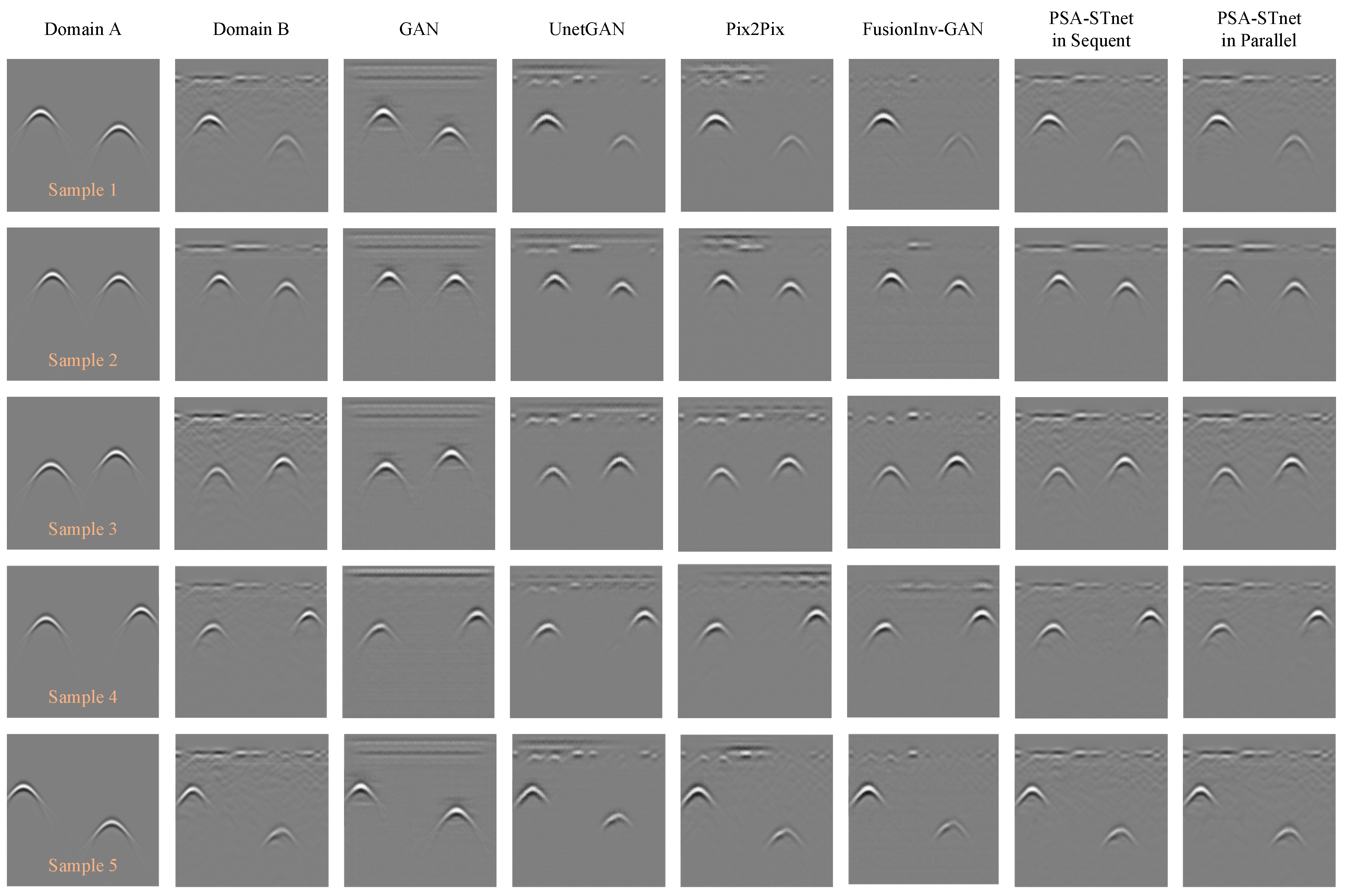
In the style transfer experiment, this study trains the GAN, the UnetGAN, the Pix2Pix, the FusionInv-GAN, and the PSA-STnet in sequence, as well as the PSA-STnet in parallel, to verify the advantages of the PSA-STnet. In the results section, five samples as shown in Figure 11 are presented.
The simulated clutter-free images (Domain A) of five samples in Figure 10 are presented again in Figure 11, and the subsequent column shows the simulated images with a mess of clutter (Domain B). The objective of the six methods is to accurately map the source Domain A to the target Domain B. As depicted in Figure 11, among the five samples, the GAN misidentifies the interference at the top of the B-scan image as a certain unexpected regular target. Moreover, in sample 1, the echo intensities of the two metal pipe targets are significantly different. However, the GAN is not sensitive to the hyperbolic echo intensity and exhibits an obvious blurring effect at the metal pipe locations. It neither stably preserves the source domain information nor effectively learns the target domain clutter distribution features, showing weak ability in both aspects. In contrast, the UnetGAN overcomes this drawback thanks to the decoder and encoder structures in the Unet generator. However, in the generator, skip connections transmit shallow-layer hyperbolic texture features directly to the decoder, lacking a mechanism to distinguish clutter from hyperbolic target features. Then it tends to preserve more information from the source domain rather than learning that from the target domain, leading to its failure in accurately generating the clutter at the top of B-scan images. Concurrently, it generates clutter as small metal pipe targets. In comparison, Pix2Pix slightly mitigates the generation of such undesired clutter at the top of B-scan images. However, it also tends to preserve more information from the source domain rather than learning that from the target domain. FusionInv-GAN, meanwhile, though it further enhances the tendency to learn the target domain heterogeneous medium clutter distribution and better preserves the source domain target hyperbolic structure, still falls short in misidentifying the clutter as small metal pipe targets due to insufficient ability to distinguish source domain target features from target domain clutter. More favorably, the PSA-STnet, whether in sequent or parallel arrangement, is capable of adaptively balancing the tendency to retain source domain information and learn target domain information, effectively avoiding the misidentification of interference as targets. Additionally, it has a keen perception ability regarding the differences in the echo intensities of metal pipe targets and is more accurate in handling the hyperbolic echo intensity.
Similar to the image translation task, the PSA-STnet in sequence and the PSA-STnet in parallel have rather close visualization results. In this paper, the MSE, PSNR, and SSIM metrics are employed to quantify their performance. As shown in Table 3, the FDTD is used as a benchmark to evaluate the effectiveness of the PSA-STnet. For FDTD itself, MSE, PSNR, and SSIM are 0, +∞, and 1, respectively. The results corresponding to both the PSA-STnet in sequence and in parallel are evidently superior to those of the GAN and UnetGAN. Among them, the PSA-STnet in parallel performs the best, with the MSE, PSNR, and SSIM reaching 4.806, 41.313 dB, and 0.987, respectively.
On the other hand, in Table 2 and Table 3, it is shown that the proposed two-step forward modeling strategy is capable of generating high-quality B-scan images from scene layout images, exhibiting a performance similar to that of the FDTD solver. However, as presented in Table 4, the FDTD method requires 292.58 s to produce a B-scan image of homogeneous medium (clutter-free) and 486.46 s for heterogeneous medium (a mess of clutter). In contrast, the proposed method only takes 0.06 s to generate a B-scan image of homogeneous medium and 0.225 s (the sum of the time cost by the image translation and style transfer models) for heterogeneous medium. The proposed two-step forward modeling strategy can generate a large number of high-quality measured GPR B-scan images with prior information in a short time, which offers more possibilities for DL tasks such as target recognition and target detection driven by a large amount of labeled data.
More crucially, the proposed method can generate GPR data of a real-world heterogeneous medium that cannot be accurately modeled by the FDTD solver, which will be verified in the real-world experiments in Section 4.

4. Real-World Experimental Verification

In real-world scenarios involving unknown dielectric constants or unquantifiable medium inhomogeneities, it is impossible to construct a precise medium model for FDTD; thus, FDTD cannot reliably simulate real-world heterogeneous medium scenes. This is primarily because FDTD relies on precise and explicit descriptions of the spatial distribution of medium parameters (e.g., dielectric constant, conductivity) within the computational domain, while real-world underground heterogeneous mediums exhibit highly random and spatially varying properties that are difficult to quantify accurately. Additionally, FDTD requires extremely fine grids to capture abrupt changes in medium properties for complex heterogeneous media, leading to prohibitively high time and computational costs. This study collected a small amount of real-world GPR data, aiming to prove that the proposed method is still capable of performing simulation work under the conditions of a real-world heterogeneous medium.

4.1. Data Preparation

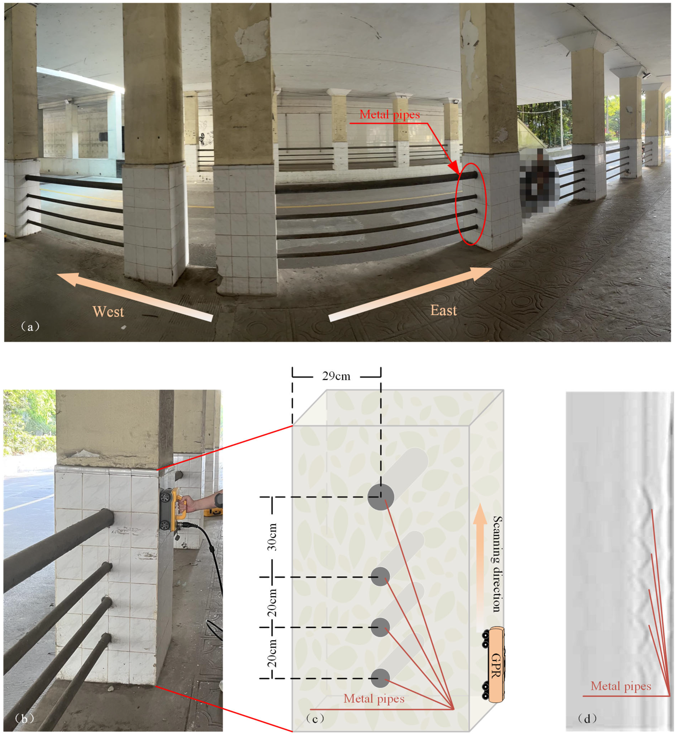
The experimental site selected for this research consists of several columnar supports beneath a bridge opening, as illustrated in Figure 12a. The cross-section of each support is square, and they are interconnected by four metal pipes structures, shown in Figure 12b. These four metal pipes are arranged in a column. Among them, the diameter of the uppermost metal pipe is 8 cm, while the diameters of the remaining three metal pipes are 5 cm each. The distance between this column of metal pipes and the left and right sides of the supports is 29 cm. The top metal tube and the second metal tube are spaced 30 cm apart, and the second, third, and fourth ones are arranged at equal intervals with a spacing of 20 cm, as depicted in Figure 12c. The main medium surrounding them is concrete.
During the data acquisition process, a GPR system with a working frequency of 1.5 GHz was employed to collect pulse signals. The pulse repetition frequency of this system was set to 128 Hz, and the detection depth could reach 3 to 50 cm. In the scanning results presented in Figure 12d, the B-scan image contains four complete hyperbolic targets of metal pipes. For better presentation and comparison, the visualization of this image and its corresponding results will be rotated 90° to the left subsequently.
In real-world experiment, the image translation task is consistent with the simulation experiment, while in the style transfer task, the target domain is replaced with real-world measured GPR B-scan images. For the forward modeling of the real-world experiment, only scene layout images and real-world measured GPR B-scan images need to be prepared. The forward process is shown in Figure 13. Taking Figure 12c as an example, a metal pipe scene layout diagram is drawn, and a simulated clutter-free image (Domain A) is obtained after passing through the trained PSA-ITnet. Then, Domain A is regarded as the source image domain, and the real-world measured GPR images (Domain B) are regarded as the target domain to train the style transfer network PSA-STnet. Finally, the GPR measured image that conforms to the real heterogeneous underground medium is generated under the unsupervised condition using the simulated clutter-free image. Regarding the details of the real-world dataset, there are two scene layout images, corresponding respectively to a single metal pipe with a diameter of 5 cm and 8 cm. After passing through the trained PSA-ITnet, two simulated clutter-free images are obtained. To avoid overfitting during the training of PSA-STnet, a random translation operation is performed on these two Domain A images, and finally 156 Domain A samples are obtained. In addition, a total of 28 real-world measured GPR B-scan images are obtained, from which 112 slices containing a single metal pipe are derived. Among these slices, 28 correspond to metal pipe samples with a diameter of 8 cm, and the remaining 84 are B-scan image slices of metal pipe samples with a diameter of 5 cm.

4.2. Experimental Verification

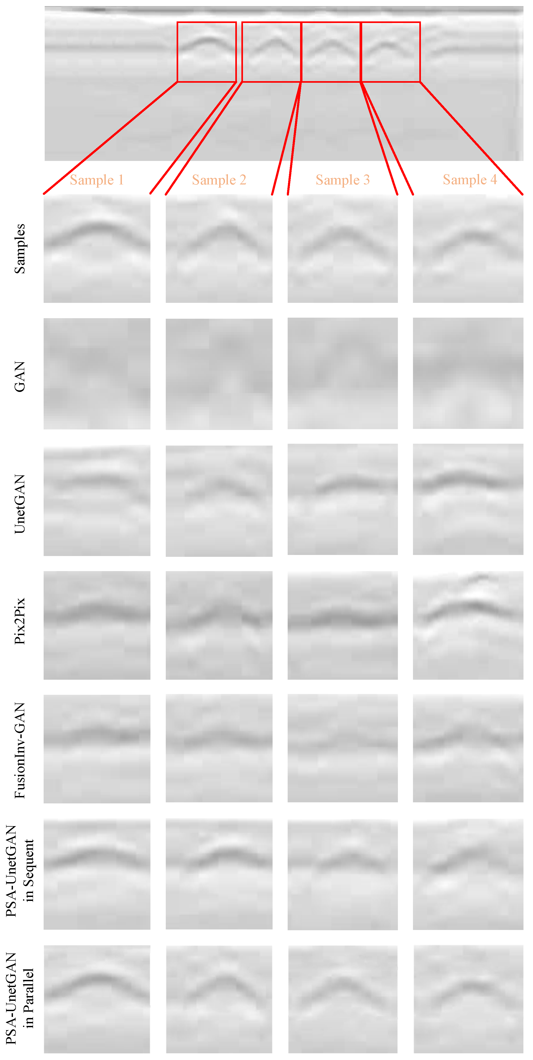
The purpose of the real-world experimental verification is to demonstrate that the proposed method can overcome the drawback of traditional numerical simulation methods, which are unable to accurately model a heterogeneous medium and thus cannot simulate complex real-world scenarios. In this paper, four metal pipe targets are selected as samples in Figure 12d to assess the effectiveness of the proposed method. Figure 14 presents the visualization results of the six methods. Among them, the GAN can hardly generate a clear target structure, let alone conform to the heterogeneous medium distribution of the target domain. The UnetGAN maps the simulated clutter-free image to the target domain, but to some extent, it impairs the information of the metal pipes. In sample 4, Pix2Pix demonstrates poor performance in generating clutter in the top of B-scan image. By contrast, FusionInv-GAN produces background clutter that aligns with the medium distribution characteristics, yet it exhibits insufficient robustness in generating hyperbolic structures. The implantation of PSA makes the PSA-STnet perform more satisfactorily compared to GAN, UnetGAN, and FusionInv-GAN. From the visualization results in Figure 14, both the sequential and parallel structures of PSA-STnet can effectively retain metal pipe targets and generate clutter backgrounds conforming to heterogeneous medium distribution, but the parallel structure shows a clear advantage in fitting real samples: its generated metal pipe hyperbolic structures are more consistent with the actual shape and edge sharpness of real targets, and the background clutter distribution is closer to the noise distribution of real GPR B-scan images, while the sequential structure’s hyperbolic edges of partial metal pipe targets are slightly blurred, making it less aligned with real scenarios.
Furthermore, this paper quantitatively assesses the effectiveness of the proposed method using MSE, PSNR, and SSIM. As shown in Table 5, the performance of the six methods in real-world experiments declines compared to simulation experiments, where the GAN shows the most severe performance degradation: its MSE reaches 389.296 (representing significant pixel-level distortion), PSNR is only 22.228 dB (indicating poor signal fidelity), and SSIM is 0.751 (reflecting obvious loss of target structural consistency). UnetGAN, while also experiencing performance decline, outperforms the GAN notably: its MSE is reduced to 127.609 (a 67.2% relative reduction compared to the GAN), PSNR is increased to 27.072 dB (4.844 dB higher than the GAN), and SSIM is improved to 0.904 (a 20.4% relative enhancement over the GAN). Among all methods, the PSA-STnet exhibits less performance degradation and stronger robustness, and a quantitative comparison between its sequential and parallel structures further confirms the latter’s superiority: in MSE, the parallel structure’s 33.089 is far lower than the sequential structure’s 62.890; in PSNR, the parallel structure achieves 32.934 dB, higher than the sequential structure’s 30.145 dB; in SSIM, the parallel structure’s 0.972 is higher than the sequential structure’s 0.923. This performance gap stems from their architectural differences: the parallel structure enables simultaneous interaction between CSA and SSA in the PSA module, allowing synchronous capture of channel-wise signal features and spatial-wise target/clutter distribution features without information loss during transmission; while the sequential structure processes channel and spatial attention in turn, which may lead to partial attenuation of key feature information during the sequential handover, thus reducing its alignment with real samples.

5. Conclusions

To overcome limitations of traditional numerical simulation methods in handling a complex heterogeneous medium and high time costs and meet demands of DL methods for prior information, this paper presents a two-step forward modeling strategy for GPR data based on image translation and style transfer. The PSA-ITnet model performs the image translation task, and the PSA-STnet model handles the style transfer task. In the image translation stage, the PSA-ITnet model shows good performance in understanding B-scan image longitudinal time delay characteristics. Compared to the GAN, UnetGAN, Pix2Pix, and FusionInv-GAN, it generates more accurate simulated clutter-free images. In the style transfer stage, the PSA-STnet model accurately converts simulated clutter-free images to ones conforming to heterogeneous medium distribution and characteristics, avoiding misidentifying interference as targets. Real-world experiments confirm the method’s practicability and advantages. In the complex bridge support structure scenario, the PSA-STnet precisely preserves metal pipe target information and generates GPR images matching real heterogeneous medium distribution well. The MSE, PSNR, and SSIM of PSA-STnet (in parallel) are 33.089, 32.934 dB, and 0.972, respectively, showing strong robustness compared to simulation experiments.
Regarding time cost, the FDTD method takes 292.58 s to generate a B-scan image in a homogeneous medium and 486.46 s in a heterogeneous medium, while the proposed method needs only 0.06 s for a homogeneous medium image and 0.225 s for a heterogeneous medium image (total of image translation and style transfer times).
In conclusion, compared with numerical simulation methods, under the preset heterogeneous medium conditions, the proposed two-step forward modeling strategy can achieve a hundred-fold improvement in time efficiency with a slight sacrifice in accuracy. Meanwhile, in real-world scenarios, it is still capable of rapidly generating a large number of high-quality GPR images with prior information, thus providing an efficient and reliable solution for GPR data simulation and analysis. Constrained by the scale of real-world data, the performance in real-world experiments is slightly lower than that in simulation experiments. In future research, more real-world samples could be incorporated to further enhance the accuracy. Additionally, the proposed method in this paper only conducts forward modeling for pipeline targets. Future work will further extend it to the forward modeling of non-pipeline target structures.

6. Limitations

This study did not explicitly integrate environmental factors (e.g., humidity, temperature) into either the model training process or the experimental configurations. These environmental variables exert a measurable influence on the dielectric constant of subsurface media: specifically, elevated humidity levels increase the dielectric constant of soil and concrete, which in turn induces shifts in the hyperbolic time delays observed in GPR B-scan images. Concurrently, temperature fluctuations may trigger physical changes in the subsurface medium, such as cracking or surface condensation. Collectively, these environmental-induced alterations disrupt the geometric-feature mapping that the proposed PSA-ITnet and PSA-STnet models are trained to learn.
Under dynamic real-world scenarios (e.g., during rainy seasons or periods of extreme temperatures), the absence of environmental factor consideration in the model and experimental design may lead to three critical issues: (1) misalignment of hyperbolic signatures in GPR data, which are essential for target detection; (2) inaccuracies in clutter simulation, thereby compromising the model’s ability to distinguish target signals from background noise; and (3) reduced preservation of target-related features. Ultimately, these issues undermine the framework’s robustness when deployed in unconstrained, real-world applications where environmental conditions are variable and uncontrollable.

Author Contributions

Formal analysis, Z.G., Z.H. and M.S.; methodology, Z.G. and Y.G.; validation, Z.G., Z.H. and M.S.; resources, Y.G., X.L., Z.G., M.S. and Z.H.; writing—original draft preparation, Z.G.; writing—review and editing, Z.G. and Y.G. All authors have read and agreed to the published version of the manuscript.

Funding

This work was supported by the National Key Research and Development Program of China under Grant 2021YFA0715400.

Data Availability Statement

The original contributions presented in this study are included in the article. Further inquiries can be directed to the corresponding author.

Conflicts of Interest

The authors declare no conflicts of interest.

References

  1. Yamaguchi, T.; Mizutani, T.; Meguro, K.; Hirano, T. Detecting Subsurface Voids from GPR Images by 3-D Convolutional Neural Network Using 2-D Finite Difference Time Domain Method. IEEE J. Sel. Top. Appl. Earth Observ. Remote Sens. 2022, 15, 3061–3073. [Google Scholar] [CrossRef]
  2. Lu, X.; Song, A.; Qian, R.; Liu, L. Anisotropic Reverse-Time Migration of Ground-Penetrating Radar Data Collected on the Sand Dunes in the Badain Jaran Desert. IEEE J. Sel. Top. Appl. Earth Observ. Remote Sens. 2018, 11, 647–654. [Google Scholar] [CrossRef]
  3. Ma, Y.; Lei, W.; Pang, Z.; Zheng, Z.; Tan, X. Rebar Clutter Suppression and Road Defects Localization in GPR B-Scan Images Based on SuppRebar-GAN and EC-Yolov7 Networks. IEEE Trans. Geosci. Remote Sens. 2024, 62, 1–14. [Google Scholar] [CrossRef]
  4. Kaur, P.; Dana, K.J.; Romero, F.A.; Gucunski, N. Automated GPR Rebar Analysis for Robotic Bridge Deck Evaluation. IEEE Trans. Cybern. 2016, 46, 2265–2276. [Google Scholar] [CrossRef]
  5. Liu, B.; Ren, Y.; Liu, H.; Xu, H.; Wang, Z.; Cohn, A.; Jiang, P. GPRInvNet: Deep Learning-Based Ground-Penetrating Radar Data Inversion for Tunnel Linings. IEEE Trans. Geosci. Remote Sens. 2021, 59, 8305–8325. [Google Scholar] [CrossRef]
  6. Porsani, J.; Navarro, A.; Rangel, R.; Neto, A.; Lima, L.; Stangari, M.; Souza, L.; Santos, V. GPR survey on underwater archaeological site: A case study at Jenipapo stilt village in the eastern Amazon region, Brazil. J. Archaeol. Sci. Rep. 2023, 51, 104114. [Google Scholar] [CrossRef]
  7. Liu, Y.; Shi, Z.; Wang, B.; Yu, T. GPR impedance inversion for imaging and characterization of buried archaeological remains: A case study at Mudu city cite in Suzhou, China. J. Appl. Geophys. 2018, 148, 226–233. [Google Scholar] [CrossRef]
  8. Lopera, O.; Slob, E.C.; Milisavljevic, N.; Lambot, S. Filtering Soil Surface and Antenna Effects From GPR Data to Enhance Landmine Detection. IEEE Trans. Geosci. Remote Sens. 2007, 45, 707–717. [Google Scholar] [CrossRef]
  9. Zhou, H.; Feng, X.; Dong, Z.; Liu, C.; Liang, W. Multiparameter Adaptive Target Classification Using Full-Polarimetric GPR: A Novel Approach to Landmine Detection. IEEE J. Sel. Top. Appl. Earth Observ. Remote Sens. 2022, 15, 2592–2606. [Google Scholar] [CrossRef]
  10. Benedetto, A.; Benedetto, F.; De Blasiis, M.R.; Giunta, G. Reliability of signal processing technique for pavement damages detection and classification using ground penetrating radar. IEEE Sens. J. 2005, 5, 471–480. [Google Scholar] [CrossRef]
  11. Zou, L.; Liu, H.; Alani, A.M.; Fang, G. Surface Permittivity Estimation of Southern Utopia Planitia by High-Frequency RoPeR in Tianwen-1 Mars Exploration. IEEE Trans. Geosci. Remote Sens. 2024, 62, 2002809. [Google Scholar] [CrossRef]
  12. Alsharahi, G.; Faize, A.; Louzazni, M.; Mostapha, A.M.M.; Bayjja, M.; Driouach, A. Detection of cavities and fragile areas by numerical methods and GPR application. J. Appl. Geophys. 2019, 164, 225–236. [Google Scholar] [CrossRef]
  13. Yee, K.S. Numerical solution of initial boundary value problems involving Maxwell’s equations in isotropic media. IEEE Trans. Antennas Propag. 1966, 14, 302–307. [Google Scholar]
  14. Di, Q.; Wang, M. Migration of ground-penetrating radar data with a finite-element method that considers attenuation and dispersion. Geophysics 2004, 69, 472–477. [Google Scholar] [CrossRef]
  15. Liu, H.; Dai, D.; Zou, L.; He, Q.; Meng, X.; Chen, J. Refined Modeling of Heterogeneous Medium for Ground-Penetrating Radar Simulation. Remote Sens. 2024, 16, 3010. [Google Scholar] [CrossRef]
  16. Liu, Q.; Fan, G. Simulations of GPR in dispersive media using a frequency-dependent PSTD algorithm. IEEE Trans. Geosci. Remote Sens. 1999, 37, 2317–2324. [Google Scholar]
  17. Zarei, S.; Oskooi, B.; Amini, N.; Dalkhani, A.R. 2D spectral element modeling of GPR wave propagation in inhomogeneous media. J. Appl. Geophys. 2016, 133, 92–97. [Google Scholar] [CrossRef]
  18. Ma, Y.; Song, X.; Li, Z.; Li, H.; Qu, Z. A Prior Knowledge-Guided Semi-Supervised Deep Learning Method for Improving Buried Pipe Detection on GPR Data. IEEE Trans. Geosci. Remote Sens. 2024, 62, 4508015. [Google Scholar] [CrossRef]
  19. Jin, A.; Chen, C.; Yang, B.; Zou, Q.; Wang, Z.; Yan, Z. GPR-Former: Detection and Parametric Reconstruction of Hyperbolas in GPR B-Scan Images with Transformers. IEEE Trans. Geosci. Remote Sens. 2024, 62, 4507113. [Google Scholar] [CrossRef]
  20. Kim, N.; Kim, S.; An, Y.-K.; Lee, J.-J. Triplanar Imaging of 3-D GPR Data for Deep-Learning-Based Underground Object Detection. IEEE J. Sel. Topics Appl. Earth Observ. Remote Sens. 2019, 12, 4446–4456. [Google Scholar] [CrossRef]
  21. Dai, Q.; Lee, Y.H.; Sun, H.-H.; Ow, G.; Yusof, M.L.M.; Yucel, A.C. DMRF-UNet: A Two-Stage Deep Learning Scheme for GPR Data Inversion Under Heterogeneous Soil Conditions. IEEE Trans. Antennas Propagat. 2022, 70, 6313–6328. [Google Scholar] [CrossRef]
  22. Wang, X.; Yuan, G.; Meng, X.; Liu, H. FusionInv-GAN: Advancing GPR Data Inversion With RTM-Guided Deep Learning Techniques. IEEE Trans. Geosci. Remote Sens. 2024, 62, 5930511. [Google Scholar] [CrossRef]
  23. Wu, Y.; Shen, F.; Zhang, M.; Miao, Y.; Wan, T.; Xu, D. A novel FDTD-based 3-D RTM imaging method for GPR working on dispersive medium. IEEE Trans. Geosci. Remote Sens. 2022, 60, 1002813. [Google Scholar] [CrossRef]
  24. Ni, Z.-K.; Shi, C.; Pan, J.; Zheng, Z.; Ye, S.; Fang, G. Declutter-GAN: GPR B-Scan Data Clutter Removal Using Conditional Generative Adversarial Nets. IEEE Geosci. Remote Sens. Lett. 2022, 19, 4023105. [Google Scholar] [CrossRef]
  25. Kayacan, Y.E.; Erer, I. A Vision-Transformer-Based Approach to Clutter Removal in GPR: DC-ViT. IEEE Geosci. Remote Sens. Lett. 2024, 21, 3505105. [Google Scholar] [CrossRef]
  26. Liu, Z.; Lin, Y.; Cao, Y.; Hu, H.; Wei, Y.; Zhang, Z.; Lin, S.; Guo, B. Swin transformer: Hierarchical vision transformer using shifted windows. In Proceedings of the 2021 IEEE/CVF International Conference on Computer Vision (ICCV), Montreal, BC, Canada, 10–17 October 2021; pp. 10012–10022. [Google Scholar]
  27. Wang, C.J.; Rost, N.S.; Golland, P. Spatial-Intensity Transforms for Medical Image-to-Image Translation. IEEE Trans. Med. Image 2023, 42, 3362–3373. [Google Scholar] [CrossRef]
  28. Ronneberger, O.; Fischer, P.; Brox, T. U-Net: Convolutional networks for biomedical image segmentation. In Proceedings of the 18th International Conference on Medical Image Computing and Computer-Assisted Intervention, Munich, Germany, 5–9 October 2015; pp. 234–241. [Google Scholar]
  29. Liu, H.; Liu, F.; Fan, X.; Huang, D. Polarized self-attention: Towards high-quality pixel-wise mapping. Neurocomputing 2022, 506, 158–167. [Google Scholar] [CrossRef]
  30. Zhang, Y.; Zhang, Y.; Cai, W. A Unified Framework for Generalizable Style Transfer: Style and Content Separation. IEEE Trans. Image Process. 2020, 29, 4085–4098. [Google Scholar] [CrossRef]
  31. Zhu, J.; Park, T.; Isola, P.; Efros, A.A. Unpaired image-to-image translation using cycle-consistent adversarial networks. In Proceedings of the 2017 IEEE International Conference on Computer Vision (ICCV), Venice, Italy, 22–29 October 2017; pp. 2242–2251. [Google Scholar]
  32. Behera, A.P.; Prakash, S.; Khanna, S.; Nigam, S.; Verma, S. CNN-Based Metrics for Performance Evaluation of Generative Adversarial Networks. IEEE Trans. Artif. Intell. 2024, 5, 5040–5049. [Google Scholar] [CrossRef]
  33. Yang, B.; Rappaport, C. Response of realistic soil for GPR applications with 2-D FDTD. IEEE Trans. Geosci. Remote Sens. 2001, 39, 1198–1205. [Google Scholar] [CrossRef]
  34. Wei, X.-K.; Zhang, X.; Diamanti, N.; Shao, W.; Sarris, C.D. Subgridded FDTD Modeling of Ground Penetrating Radar Scenarios Beyond the Courant Stability Limit. IEEE Trans. Geosci. Remote Sens. 2017, 55, 7189–7198. [Google Scholar] [CrossRef]
  35. Takekura, S.; Miyamoto, H.; Kobayashi, M. Detecting Lunar Subsurface Water Ice Using FMCW Ground Penetrating Radar: Numerical Analysis with Realistic Permittivity Variations. Remote Sens. 2025, 17, 1050. [Google Scholar] [CrossRef]
  36. Mao, L.; Wang, X.; Chi, Y.; Pang, S.; Wang, X.; Huang, Q. A Three-Dimensional FDTD(2,4) Subgridding Algorithm for the Airborne Ground-Penetrating Radar Detection of Landslide Models. Remote Sens. 2025, 17, 1107. [Google Scholar] [CrossRef]
  37. Cheng, Q.; Cui, F.; Dong, G.; Wang, R.; Li, S. A Method of Reconstructing Ground Penetrating Radar Bscan for Advanced Detection Based on High-Order Synchrosqueezing Transform. IEEE Trans. Geosci. Remote Sens. 2024, 62, 5910313. [Google Scholar] [CrossRef]
  38. McDonald, T.; Plattner, A.; Warren, C.; Robinson, M.; Tian, G. 3-D Visualization of New Hybrid-Rotational Ground-Penetrating Radar for Subsurface Inspection of Transport Infrastructure. IEEE Trans. Geosci. Remote Sens. 2025, 63, 5101613. [Google Scholar] [CrossRef]
  39. Zhang, Z.; Sun, W.; Min, X.; Wang, T.; Lu, W.; Zhai, G. A Full-Reference Quality Assessment Metric for Fine-Grained Compressed Images. In Proceedings of the 2021 International Conference on Visual Communications and Image Processing (VCIP), Munich, Germany, 5–8 December 2021; pp. 1–4. [Google Scholar]
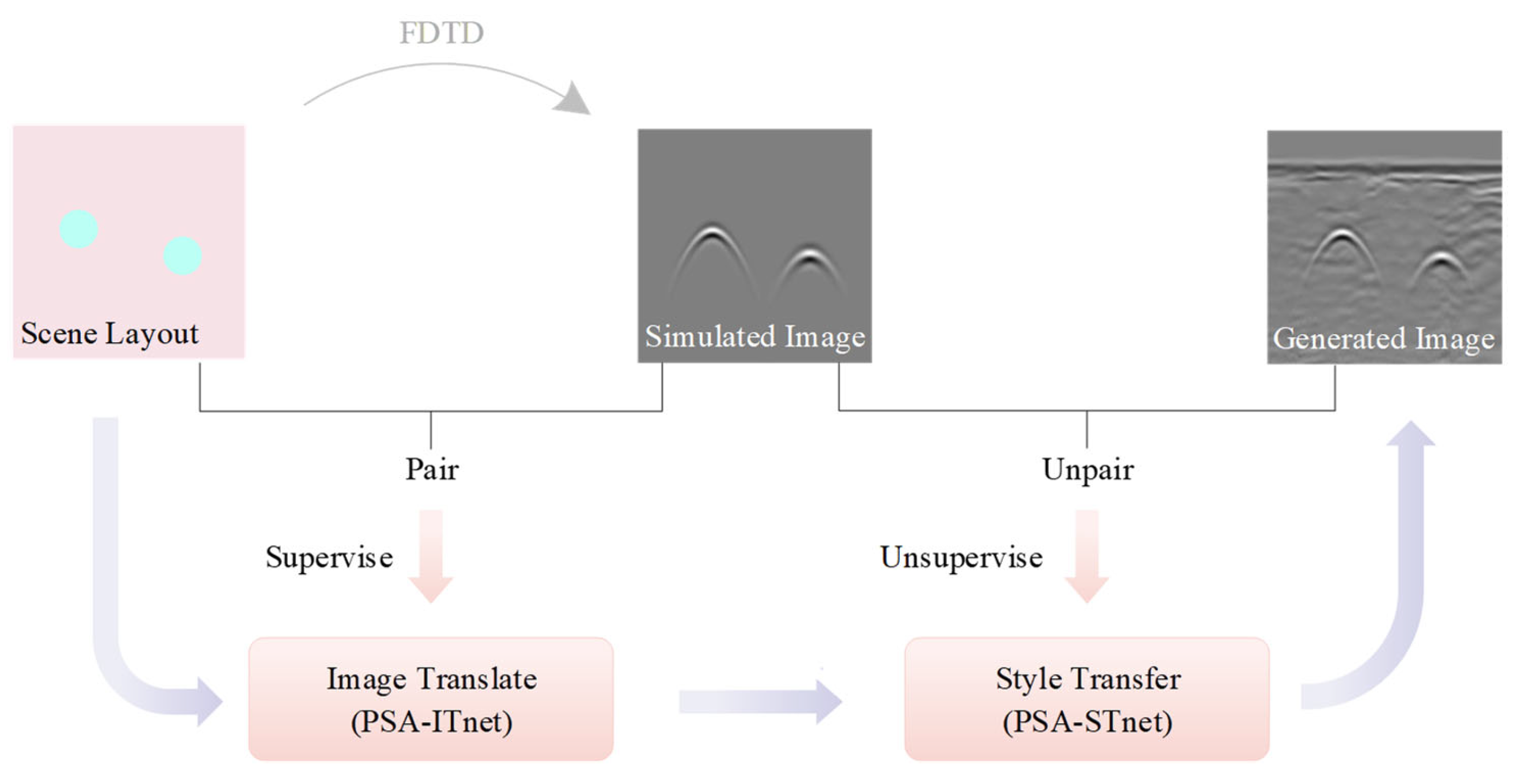
Figure 1. Flow chart of the Two-Step forward modeling strategy.
Remotesensing 17 03215 g001
Figure 2. Network structure of two-step forward modeling. In Step 1: Image Translation, the structure of PSA-ITnet is illustrated; In Step 2: Style Transfer, the structure of PSA-STnet is illustrated.
Remotesensing 17 03215 g002
Figure 5. Illustration of PSA in parallel.
Remotesensing 17 03215 g005
Figure 6. Illustration of PSA in sequence.
Remotesensing 17 03215 g006
Figure 7. Design of Simulation Experiment Dataset. From left to right, the samples are the scene layout images, simulation clutter-free images (Domain A), simulation clutter images with two metal pipes (Domain B), and simulation clutter images with one metal pipe (Domain B), respectively.
Remotesensing 17 03215 g007
Figure 8. Schematic diagram of samples and quantities required for training PSA-ITnet in simulation experiment. (a) Simulation scenarios for train set. (b) Simulation scenarios for test set. (b) and (d) are simulated image corresponds to (a) and (c), respectively.
Remotesensing 17 03215 g008
Figure 9. Schematic diagram of samples and quantities required for training PSA-STnet in simulation experiment. (ac) are simulation scenarios for train set. (a) is scene layout in homogeneous medium, while (b,c) are in heterogeneous medium. (df) are simulated image corresponds to (a), (b) and (c), respectively. (g,h) are simulation scenarios for test set. (g) is scene layout in homogeneous medium, while (h) is in heterogeneous medium. (i,j) are simulated image corresponds to (g) and (h), respectively.
Remotesensing 17 03215 g009
Figure 10. Visualization results of six image translations.
Remotesensing 17 03215 g010
Figure 11. Visualization results of six style transfer methods in simulation experiment.
Remotesensing 17 03215 g011
Figure 12. Real-world GPR dataset project. (a) Scenario picture. (b,c) are the actual data collection picture and the schematic diagram of data collection, respectively. (d) is the collected real-world GPR B-Scan image.
Remotesensing 17 03215 g012
Figure 13. Schematic diagram of samples and quantities required for forward modeling in real-world experiment.
Remotesensing 17 03215 g013
Figure 14. Visualization results of six style transfer methods in real-world experiment.
Remotesensing 17 03215 g014
Table 1. Metal Pipes and dielectric layer material information.
MaterialsSize (cm)Dielectric Constant
Air51
Underground medium959
Metal pipes ϕ 5~20
Table 2. Quantitative evaluation results of image translation task in simulation experiments.
FDTDGANUnetGANPix2PixFusionInv-GANPSA-ITnet
in Sequent
PSA-ITnet
in Parallel
MSE095.23218.73627.84014.1814.3524.182
PSNR (dB)+∞28.34335.40433.68436.61441.74441.917
SSIM10.8640.9150.9040.9230.9500.953
Table 3. Quantitative evaluation results of style transfer tasks in simulation experiments.
FDTDGANUnetGANPix2PixFusionInv-GANPSA-STnet
in Sequence
PSA-STnet
in Parallel
MSE0228.57835.15333.43910.9105.1524.806
PSNR (dB)+∞24.54032.67132.87237.75341.01141.313
SSIM10.7620.8540.8610.9070.9790.987
Table 4. Comparison of timeliness between two forward modeling methods.
MethodsTime Cost of a B-Scan Image (s)
FDTDHomogeneous medium292.580
Heterogeneous medium486.460
Proposed methodPSA-ITnet0.060
PSA-STnet0.165
Table 5. Quantitative evaluation results of style transfer tasks in real-world experiments.
GANUnetGANPix2PixFusionInv-GANPSA-STnet
in Sequence
PSA-STnet
in Parallel
MSE389.296127.609135.284144.48762.89033.089
PSNR (dB)22.22827.07226.81826.53330.14532.934
SSIM0.7510.9040.8580.8460.9230.972
Disclaimer/Publisher’s Note: The statements, opinions and data contained in all publications are solely those of the individual author(s) and contributor(s) and not of MDPI and/or the editor(s). MDPI and/or the editor(s) disclaim responsibility for any injury to people or property resulting from any ideas, methods, instructions or products referred to in the content.