Target Detection in Sea Clutter Background via Deep Multi-Domain Feature Fusion

Highlights

What are the main findings?

• Effectively integrating sea clutter radar echo features in the time, frequency, fractal, and polarization domains demonstrates that multi-feature fusion can enhance the separability of sea clutter and target samples, which helps overcome the limitations of single-feature domain detection methods in different scenarios.
• Applying deep learning networks to sea surface low-altitude small target detection and designing effective false alarm control methods tailored to specific application scenarios.

What is the implication of the main finding?

• This method provides a reliable approach for detecting sea surface targets in complex scenarios.
• This method offers an effective framework and ideas for the application of deep learning in sea surface remote sensing and intelligent detection.

Abstract

The complex and dynamic nature of the marine environment poses significant challenges for sea surface target detection. Traditional methods relying on single-domain features suffer from performance degradation under varying conditions. To address this limitation, a multi-domain polarization-aware feature fusion network capable of controlling the false alarm rate (MP-FFN) for robust sea surface target detection is proposed in this paper. The proposed method first extracts discriminative radar echo features from time, frequency, fractal, and polarization domains. Subsequently, autoencoder-based intra-domain network is employed to reduce feature dimensionality while minimizing information loss. These compressed features are then fused through a multi-layer perceptron (MLP)-based inter-domain network, enabling comprehensive cross-domain correlation learning. Moreover, a controllable false alarm rate is achieved through a customized loss function. Extensive experiments on the IPIX radar dataset demonstrate that the proposed method outperforms traditional feature-based detection methods, exhibiting superior robustness and detection accuracy in diverse marine environments.

1. Introduction

Maritime target detection, a crucial subfield of radar applications, possesses significant research value for both military and civilian domains. As radar resolution increases, traditional detection methods often prove inadequate for modern systems. Within complex ocean clutter environments, radar performance in detecting small maritime targets is degraded by clutter, particularly the sea spike phenomenon, which frequently causes false alarms. Furthermore, complex, nonlinear sea surface variations, influenced by environmental factors such as meteorological and geographical conditions, undermine traditional detection techniques reliant on target energy accumulation [1,2]. Consequently, developing novel target detection algorithms to overcome these challenges is imperative.

Recently, a variety of methods have been proposed to address the challenge of small target detection, especially in the context of sea clutter. Existing methods can be categorized into two main types: model-driven and feature-driven target detection methods [1]. The model-driven approach assumes that sea clutter follows a specific statistical distribution, transforming target detection into a binary hypothesis test through hypothesis testing. These methods possess significant engineering application value. However, with advancements in high-resolution radar, the non-Gaussian, nonlinear, and non-stationary properties of sea clutter render the detection model indescribable using concrete mathematical formulas, thus posing a significant challenge in modeling [2,3].

Feature-driven detection methods offer new insights [4,5,6]. In [7], the autoregressive (AR) spectrum domain is utilized, leveraging its multifractal correlation properties and refined fractal characteristics for detection. However, fractal-based detectors typically require several seconds to achieve satisfactory performance, which limits their real-time applicability. In [8], a tri-feature-based detector was introduced, initiating a new framework for multidimensional feature detection. Nevertheless, this method focuses solely on the time-domain characteristics of sea clutter, resulting in constrained detection performance. In [9], the connected density of graph (CDG) approach is developed based on amplitude spectrum series, integrating geometric correlation and spectral characteristics to enhance detection. Disperse relative entropy (DRE), proposed in [10] after a two-stage clutter suppression process, not only delivers competitive performance but also reduces computational complexity. Although the method based on time–frequency domain characteristics fulfills the requirements of practical radar systems for rapid detection and simplicity, it is significantly influenced by sea conditions. Therefore, different feature domains have their respective applications. When the detection scenario changes, feature detection based on a single domain often exhibits certain limitations, resulting in a decline in detection performance. The varying manifestations of sea clutter across multiple domains facilitate more effective detection of sea surface targets in diverse scenarios.

In feature-driven methods, multi-feature fusion detection has emerged as the mainstream approach for sea surface target detection [11,12,13,14]. Feature fusion can reduce redundancy among features while ensuring that the classifier obtains sufficient relevant target information. Generally, feature fusion methods fall into two primary categories. The first is constraint-based fusion, which often involves concatenating features followed by dimensionality reduction methods such as Principal Component Analysis (PCA) [15,16]. However, PCA is mainly effective for normally distributed data, limiting its broader applicability. Alternatively, multi-kernel learning has been introduced to make better use of diverse feature sets, often yielding improved classifier performance compared to single-kernel Support Vector Machines (SVM) [17,18]. Ref. [17] proposed an SVM-based approach, but it is restricted by a minimum achievable false alarm rate of 0.01, which does not fully meet practical requirements. In [18], a method combining k-means clustering and OCSVM was used, but its false alarm control is dependent on the value of k, thus lacking flexibility. The second type of feature fusion method utilizes neural networks, such as autoencoder (AE) and end-to-end networks (CNNs and Transformers) [19,20,21]. AE is primarily utilized for dimensionality reduction and feature fusion, encompassing both encoding and decoding networks. The stacked autoencoder (SAE), consisting of multiple acoustic emission layers, exhibits greater representational power compared to single-layer AE, thus frequently employed in fusion tasks [19]. Ref. [20] introduces a CNN-based approach to integrate features from multiple domains of sea echoes, enhancing detection performance in intricate scenarios; however, this method has limited false alarm control capabilities. Ref. [21] presents a Transformer-based target detection technique suitable for sea surface target detection, yet it also falls short in achieving controllable false alarms.

This paper presents a multi-domain polarization-aware feature fusion network (MP-FFN) designed to process fully polarized features extracted from sea surface radar echoes. An intra-domain network fuses features within the same domain to reduce redundancy, while an inter-domain network performs secondary fusion on features from different domains to enhance feature space robustness by leveraging cross-domain complementarity. Joint optimization of intra-class and inter-class loss functions enables controllable false alarm rates. By integrating diverse, informative features from fully polarized radar echoes, the approach enhances feature space separability. Validation using real-world data confirms the method’s effectiveness in improving sea target detection under complex conditions.

The main contributions of this work are:

• The characteristics of sea clutter vary significantly under different detection scenarios, and detection methods based on single-domain sea clutter features have considerable limitations. This paper fuses sea surface echo features from four domains to somewhat overcome the issues caused by changes in detection scenarios.
• Unlike traditional approaches that depend on single-polarization data and are sensitive to polarization differences, this work utilizes fully polarized data. By analyzing echo characteristics from multiple feature domains, it captures more complete radar information, which can lead to more robust detection performance.
• An intelligent method for weak target detection amid sea clutter is presented. It employs intra-domain networks to reduce feature redundancy and inter-domain networks to effectively integrate diverse domain features. Controllable false alarm rates are achieved by optimizing loss functions. Validation on the IPIX radar dataset confirms the algorithm’s effectiveness and superiority over compared methods.

Here,

Table 1. List of notations in the MP-FFN method.

$m$: Polarization mode, $m\in \left\{hh,vv,hv,vh\right\}$. $i$: The serial number of the sample to be tested. $x(i)$: The $i$-th radar echo sample. $p(i)$: Probability of $x(i)$. $q$: Non-extensive parameter. $F_{type}$: Calculation of extracted features, $type\in \left\{PRAA,PRVE,PDPH,POTE,PE,SSC\right\}$. $J$: Loss function. $D$: Distance between samples. $\alpha$: The weight of the reconstruction loss in the intra-domain network. $\beta$: The weight of the proportional loss in the intra-domain network. $c$: The serial number of sample categories. $r$: The serial number of neurons. $k$: The serial number of hidden-layer features. $n_c$: The number of samples labeled as $c$. $h_k^c$: The hidden layer feature labeled as k at the c-th position. $\delta$: The empirical parameter of activation function. $g(\cdot )$: Activation function of the Leaky ReLU. $g_{softmax}(x_i^c)$: The probability of the i-th sample being classified as belonging to class c. $N_{total}$: The total number of samples in the test set. $T$: Detection threshold. $\kappa$: Index value corresponding to the detection threshold under a given false alarm rate. $W$: The penalty term for all parameters in the network. $Z_s$: The separability measurement function.

lists all notations in our MP-FFN model to help readers understand the dimensions of matrices and definitions of notations clearly.

The remainder of this manuscript is organized as follows: Section 2 reviews fundamental concepts of target detection in sea clutter. Section 3 presents the proposed multi-domain feature fusion network. Section 4 provides experimental results of proposed methods. Section 5 discusses the comparison between the proposed method and existing methods, as well as the convergence of the algorithm. Finally, Section 6 concludes the paper.

2. Review of Target Detection in Sea Clutter Background

Binary hypothesis testing provides a foundational model for target detection within sea clutter environments, particularly for active radar systems. This framework establishes two competing hypotheses: the null hypothesis (H₀) and the alternative hypothesis (H₁). The null hypothesis (H₀) assumes the observation cell contains only sea clutter, exhibiting statistical characteristics consistent with known clutter-only reference cells. Conversely, the alternative hypothesis (H₁) posits that the cell contains a target signal superimposed on the clutter. The resulting binary hypothesis test is formulated as follows:

$$\begin{gathered} \left\{\begin{array}{l}{H}_0:x_m(i)=c_m(i)\\ H_1:x_m(i)=c_m(i)+s_m(i)\end{array}\right. \\ \mathrm{s}.\mathrm{t}.i=1,2,\cdots ,L;m\in \{\mathrm{HH},\mathrm{HV},\mathrm{VV},\mathrm{VH}\}; \end{gathered}$$

(1)

where $x_m(i)$, $s_m(i)$, and $c_m(i)$ represent the received vector of the m-th polarization channel, the potential target echo, and the sea clutter vector within the detection cells, respectively. L is the length of radar echo data. It is important to note that the clutter vectors in the detection cells and reference cells are assumed to share the same statistical properties [22].

3. Multi-Domain Feature Fusion Network

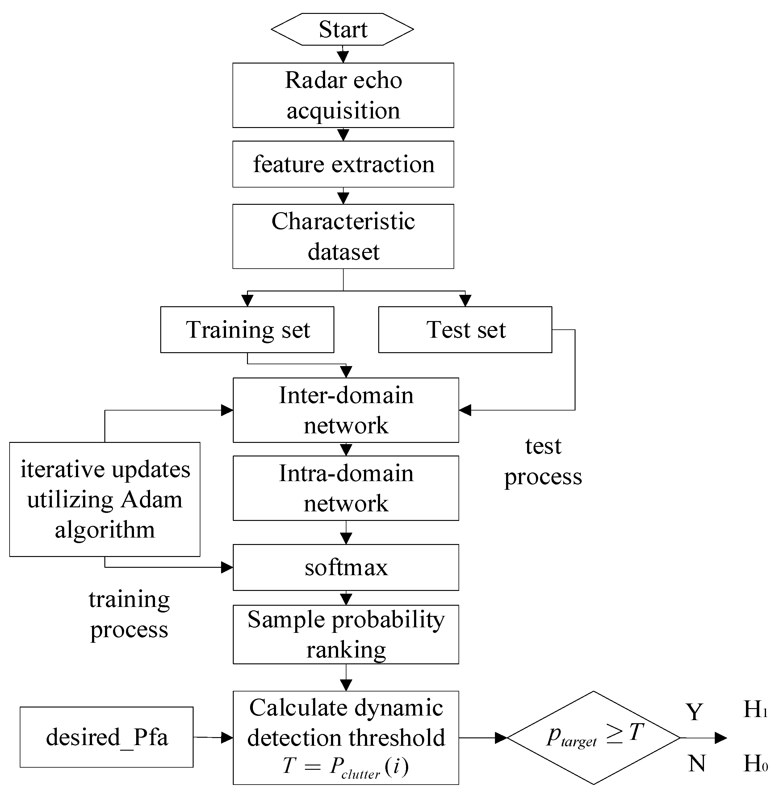
The multi-domain feature fusion network proposed in this paper consists of four parts: the feature extraction part, the intra-domain network, the inter-domain network, and the false alarm control part. Initially, six fully polarized features of the radar echo unit are extracted from the perspectives of the time, frequency, fractal, and polarization domains. Subsequently, feature fusion is carried out through a hierarchical fusion network, encompassing both intra-domain and inter-domain networks. Specifically, the intra-domain network employs an AE structure to eliminate feature redundancy within each domain while preserving key information of the features. The inter-domain network enhances the robustness of classification by fusing the intrinsic relationships between different feature domains. By optimizing the loss functions within and between classes, false alarms can be stably maintained at 0.001. The specific process is shown in Figure 1.

3.1. Multi-Domain Feature Extraction

This study extracts features from fully polarized channels across multiple domains as input variables: Full-Polarization Relative Average Amplitude (PRAA) from the time domain [4]; Full-Polarization Doppler Spectrum Vector Entropy (PRVE) and Full-Polarization Relative Doppler Peak Height (PDPH) from the Doppler domain [15]; Full-Polarization Tails Entropy (POTE) [16] from the fractal domain; and Polarization Entropy (PE) [17], along with Spherical Scattering Component (SSC) [16], from the polarization domain. To leverage information across all polarization channels, the first four features (PRAA, PRVE, PDPH, and POTE) are computed by averaging their respective values obtained from each of the four channels. PE and SSC inherently utilize polarimetric information.

(1) In the time domain, sea clutter amplitude fluctuates significantly due to wave motion, whereas target echo amplitudes are typically larger. RAA is defined as the ratio of the average amplitude of the test unit to the average amplitude of the reference unit, expressed as follows:

$$F_{RAA}\left(x_d;x_e\right)={\displaystyle \frac{\left|x_d\left(i\right)\right|}{\frac{1}{L}{\displaystyle \sum _{e=1}^L\left(\left|x_e\left(i\right)\right|\right)}}}$$

(2)

where $x_d$ and $x_e$ representing the echoes of the test unit and the reference unit with a length of L respectively. PRAA is the average RAA value of the four polarization channels HH, VV, HV, and VH. Consequently, the PRAA for target cells is generally higher than for clutter cells.

(2) In the frequency domain, within the Doppler domain, PRVE quantifies spectral characteristics related to randomness or concentration. Targets, possessing relatively stationary scattering components, tend to produce more concentrated Doppler spectra compared to the broader spectra resulting from the chaotic motion and roughness of pure clutter. This leads to higher PRVE values for target-containing units than for pure clutter units. Similarly, PDPH, reflecting Doppler kurtosis or spectral peakedness, is also higher for the more concentrated target spectrum compared to the broader clutter spectrum.

The vector entropy (VE) of the normalized Doppler spectrum is defined as follows:

$$F_{VE}(x)=-{\displaystyle \sum _{f_d}\widehat{X}(f_d})\lg \widehat{X}(f_d)$$

(3)

where $\widehat{X}(f_d)$ is the Doppler Amplitude Spectrum. The PRVE is defined as follows:

$$F_{RVE}\left(x_d;x_e\right)={\displaystyle \frac{F_{VE}\left(x_d\right)}{\frac{1}{L}{\displaystyle \sum _{e=1}^L{F}_{VE}\left(x_e\right)}}}$$

(4)

In the Doppler spectrum of the signal, the presence of target information causes more energy to be concentrated at the target’s Doppler frequency. The target cell has a sharper Doppler spectrum, and PDPH can characterize this feature, which is defined as follows:

$$F_{PDPH}={\displaystyle \frac{\max X(f_d)}{1/\#\Delta {\displaystyle \sum _{f_d\in f_{d\max }}X\left(f_d\right)}}}$$

(5)

where f_{d max} is the frequency corresponding to the peak value in the Doppler spectrum; Δ is a reference Doppler frequency interval defined as [−δ₁, −δ₂]∪[δ₂, δ₁], and #Δ represents the number of elements belonging to the set Δ. For the IPIX dataset, the parameter values of δ₁ and δ₂ are 50 Hz and 5 Hz, respectively.

(3) In the fractal domain, targets represent artificial structures lacking the inherent fractal characteristics often associated with natural sea clutter. Tsallis Entropy (TE) with the non-extensive parameter $q$, the generalization of SE, can partly reflect the nonlinear dynamic characteristics of the system [10]. The TE, $S_q$, can be defined as follows:

$$F_{POTE}={\displaystyle \sum _{i=1}^{L}p(i){\ln }_q\frac{1}{p(i)}}$$

(6)

POTE is the average TE value of the four polarization channels HH, VV, HV, and VH. This difference in structural complexity, captured by the POTE, results in higher POTE values for target cells compared to clutter cells.

(4) In the polarization domain, the PE measures the degree of randomness in the scattering mechanism. Sea clutter, particularly at very low grazing angles (reflection angles > 85°), can exhibit highly random scattering [23]. Artificial targets introduce more deterministic scattering components, thereby reducing the overall randomness. Consequently, PE values are typically higher for pure sea clutter than for cells containing targets. Conversely, the SSC quantifies the contribution of spherical scattering. While the dominant scattering mechanism in sea clutter varies with sea state, artificial targets often maintain a more pronounced and consistent spherical scattering signature. As a result, targets generally exhibit higher SSC values than sea clutter.

The non-coherent decomposition method based on polarization covariance matrix can well describe the random scattering characteristics of targets and sea clutter [24]. Based on the Pauli base matrix, the coherence matrix $M_p$ can be obtained as follows:

$$M_p={\displaystyle \sum _{d=1}^3{\lambda }_d{u}_d{u_d}^H}$$

(7)

where the terms ${\lambda }_1>{\lambda }_2>{\lambda }_3$ represent the eigenvalues of $M_p$, and $u_d$ is the eigenvector associated with the $d$-th eigenvalue.

The polarization scattering entropy (PE) is defined as follows:

$$F_{PE}=-{\displaystyle \sum _{d=1}^3{v}_d{\log }_3{v}_d}$$

(8)

where $v_d={\lambda }_d/({\lambda }_1+{\lambda }_2+{\lambda }_3)$.

The coherent decomposition method based on polarization scattering matrix can well describe the scattering structure of target and sea clutter [25]. The conversion relationship of the elements in the polarization scattering matrix under two polarization bases is given in Equation (9):

$$\left\{\begin{array}{l}{x}_{rr}=j{x}_{hv}+{\displaystyle \frac{1}{2}}(x_{hh}-x_{vv})\\ x_{ll}=j{x}_{hv}-{\displaystyle \frac{1}{2}}(x_{hh}-x_{vv})\\ x_{rl}={\displaystyle \frac{j}{2}}(x_{hh}+x_{vv})\end{array}\right.$$

(9)

Therefore, the real coefficient of SSC can be represented as follows:

$$F_{SSC}=\left|x_{rl}\right|$$

(10)

3.2. Intra-Domain Network

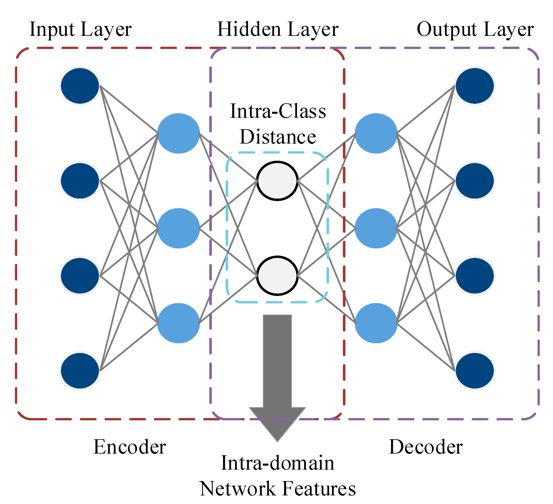
This article employs SAE as the intra-domain network, with the number of SAE layers in each feature domain determined by the quantity of features. Specifically, a greater number of features within a feature domain corresponds to a higher number of layers. Figure 2 illustrates the structure of a three-layer intra-domain network.

The loss function of this intra-domain network primarily comprises two components: the reconstruction loss $J_{reconstruction}^{domain}$, which consists of SAE reconstruction terms, and the proportional loss $J_{ratio}^{domain}$, which is formulated based on the ratio constraints between within-class and between-class variations.

$$J_{intra}^{domain}=\alpha J_{reconstruction}^{domain}+\beta J_{ratio}^{domain}$$

(11)

In this context, $\alpha ,\beta$ serves as a hyperparameter, regulating the weights assigned to the reconstruction loss and the proportional loss. The reconstruction loss within the intra-domain network solely focuses on the reconstruction of a single-feature domain:

$$J_{reconstruction}^{domain}={‖x^{domain}-{\widehat{x}}^{domain}‖}_2^2$$

(12)

where $x^{domain}$ is the input feature of domain, ${\widehat{x}}^{domain}$ is the reconstruction item corresponding to $x^{domain}$.

Proportional loss consists of intra-class distance $D_{within}^{domain}$ and inter-class distance $D_{between}^{domain}$. The calculation of $D_{within}^{domain}$ is as follows:

$$D_{within}^{domain}={\displaystyle \sum _{c=0}^{C-1}1/n_c{\displaystyle \sum _k^{n_c}{\left(h_k^c-{\overline{h}}^c\right)}^T\left(h_k^c-{\overline{h}}^c\right)}}$$

(13)

where $n_c$ denotes the number of samples labeled as $c(c=0,\dots ,C-1)$, c represents the total number of categories, $h_k^c$ signifies the hidden layer feature labeled as k at the c-th position, and ${\overline{h}}^c$ stands for the mean of the hidden layer vector features labeled as c.

The calculation of inter-class distance is as follows:

$$D_{between}^{domain}={\displaystyle \sum _{c=0}^{C-1}{\left({\overline{h}}^c-\overline{h}\right)}^T\left({\overline{h}}^c-\overline{h}\right)}$$

(14)

where $\overline{h}$ is the mean of the hidden feature vectors of all samples.

By considering both intra-class and inter-class distances, the proportional loss can be obtained as $J_{ratio}^{domain}$:

$$J_{ratio}^{domain}={\displaystyle \frac{D_{within}^{domain}}{D_{between}^{domain}}}$$

(15)

3.3. Inter-Domain Network

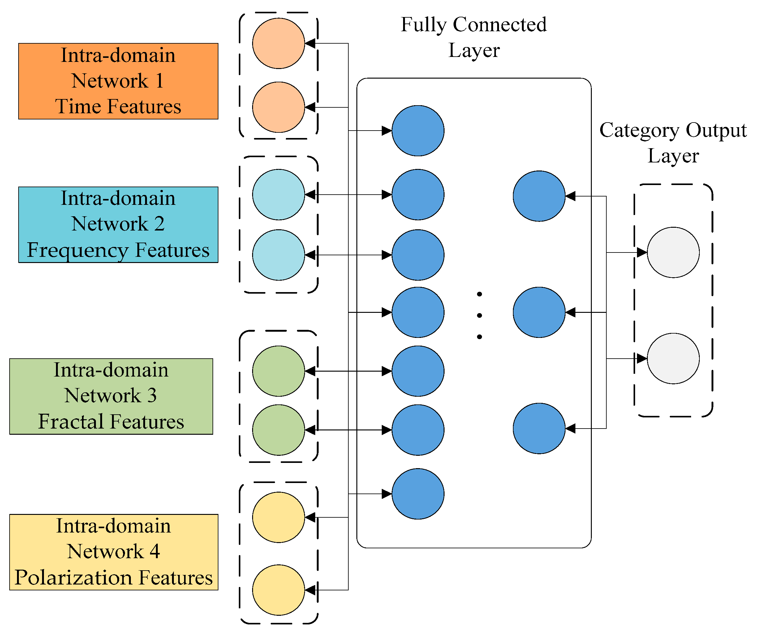
An inter-domain network is a multi-layer network designed to integrate the hidden-layer output features from multiple distinct intra-domain networks. In contrast to traditional fusion approaches, hierarchical feature fusion networks jointly optimize feature fusion and target classification. Fusion, driven by classification, can steer the fusion process toward enhanced feature separability, which in turn facilitates improved target classification with well-separated features. Consequently, inter-domain networks not only integrate diverse feature domains but also categorize targets.

Primarily, inter-domain networks consist of multi-layer perceptrons (MLPs), comprising multiple fully connected layers. Since intra-domain networks have already largely eliminated redundant information within the same feature domain, the marginal benefit of further redundancy reduction using intra-domain networks is minimal. Therefore, inter-domain networks primarily leverage the multi-layer nonlinear mappings of MLPs to progressively fuse hidden features across multiple feature domains.

Figure 3 illustrates the architecture of an inter-domain network, where the input comprises the hidden features of various feature domains after processing through their respective intra-domain networks. In the absence of prior information regarding the importance ranking of feature domains, it is advisable for the hidden-feature dimensions of all feature domains to be uniform, ensuring that the network treats all feature domains impartially. These hidden-layer nodes from all feature domains are concatenated to form a new fusion layer, as depicted in Figure 3.

The spliced fusion layer is then subjected to multiple layers of nonlinear mapping, which uses the activation function of Leaky ReLU:

$$g(x)=\left\{\begin{array}{c}x,x\ge 0\\ {\displaystyle \frac{x}{\delta }},x<0\end{array}\right.$$

(16)

where $\delta$ is the empirical parameter.

The number of neurons in the category output layer is equal to the number of categories, and the neurons in this layer are mapped using Softmax function as follows:

$$g_{softmax}(x_c)={\displaystyle \frac{\exp \left(x_c\right)}{{\displaystyle \sum _c\exp \left(x_c\right)}}}$$

(17)

where $x_c$ represents the c-th neuron in this layer, which is also bound to the c-th category. The category determined by the inter-domain network can be expressed as follows:

$$p_c=\underset{c}{\arg \max }{\displaystyle \frac{\exp \left(x_c\right)}{{\displaystyle \sum _c\exp \left(x_c\right)}}}$$

(18)

The loss function of the inter-domain network is given by the following equation:

$$J_{inter}=-{\displaystyle \frac{1}{N_{total}}}{\displaystyle \sum _{r=0}^{N_{total}-1}{\displaystyle \sum _{c=0}^{C-1}{y}_r^c\log \left(g_{softmax}(x_r^c)\right)}}$$

(19)

where $N_{total}$ represents all samples; $y_r^c$ is binary, when the label of r-th samples is c, $y_r^c=1$ in other cases $y_r^c=0$; $x_r^c$ represents the output of the r-th neuron in the network for c samples, and $g_{softmax}(x_r^c)$ represents the probability of the r-th sample being classified as class c.

3.4. Control of False Alarms

The control of false alarms in this method is achieved by adjusting the loss function. The proposed MP-FFN is an integrated network consisting of two parts: an intra-domain network and an inter-domain network. Consequently, the overall loss function comprises two components: the loss function for the intra-domain network $J_{intra}$ and the loss function for the inter-domain network $J_{inter}$. The intra-domain network is made up of four sections: the network resulting from the fusion of time-domain features via SAE, the network from the fusion of frequency-domain features via SAE, the network after the fusion of fractal-domain features via SAE, and the network following the fusion of polarization-domain features via SAE. Therefore, the total loss function for the intra-domain network can be expressed as follows:

$$J_{intra}={\displaystyle \sum _{domain}{J}_{intra}^{domain}}$$

(20)

where $domain\in \left\{time,frequency,fratal,polarization\right\}$.

The calculation for the total loss function of MP-FFN can be expressed as follows:

$$J=J_{inter}+{\displaystyle \sum _{domain}{J}_{intra}^{domain}}+{‖W‖}_2^2$$

(21)

where $W$ is the penalty term for all parameters in the network, which is the regularization constraint for the network parameters.

False alarm control is implemented by computing the Softmax function value within the loss function of the inter-domain network. Initially, the paper sorts the clutter samples output by the inter-domain network. Subsequently, it derives an adaptive decision threshold based on a preset false alarm rate. Lastly, the output values of the inter-domain network are updated according to the current parameters, optimizing the proposed network. Consequently, while adhering to the specified false alarm rate, the target detection performance is enhanced. The relevant theoretical analysis and algorithmic process are as follows:

(1)

Softmax output and sample probability representation

Assuming the output layer of the neural network employs the Softmax activation function, the output produced for any given input sample $x$ is a two-dimensional vector:

$$p(x)=[p_{clutter},p_{target}]$$

(22)

where $p_{clutter}$ represents the prediction probability of the sample being clutter, $p_{target}$ represents the predicted probability of the sample being the target, and $p_{clutter}+p_{target}=1$.

(2)

Output sample probability ranking

Sort the $p_{target}$ values of all clutter samples. Assuming the number of clutter samples is $N_{\mathrm{clutter}}$, the corresponding target probability outputs are sorted in descending order to form the following set:

$$p_{target}^{clutter}=\left\{p_{target}^{(1)},p_{target}^{(2)},p_{target}^{(3)},\dots ,p_{target}^{(N_{clutter})}\right\}$$

(23)

where $p_{target}^{(1)}\ge p_{target}^{(2)}\ge p_{target}^{(3)}\ge \dots \ge p_{target}^{(N_{clutter})}$, $p_{target}^{clutter}$ is the set of target category probability values corresponding to the clutter samples in the Softmax output.

(3)

Detection threshold setting

Assuming the desired false alarm probability is $p_{fa}^{desired}$, the decision threshold $T$ can be determined using the following formula:

$$T=P_{clutter}(\kappa )$$

(24)

$$\kappa =\max (1,[p_{fa}^{desired}·N_{clutter}])$$

(25)

The max() function ensures that the index $\kappa$ is at least 1, even at extremely low expected false alarm rates, to obtain a valid threshold. Ultimately, the $p_{target}$ values of all test samples are compared to the threshold T. If $p_{target}\ge T$, it is classified as the target; otherwise, it is classified as clutter.

(4)

Algorithm update and false alarm control process

The detection process employed in this paper consists of two parts: training and testing, encompassing the following six steps:

Step 1:

Obtain radar echo data and perform feature extraction to generate a feature dataset.

Step 2:

Divide the feature dataset into a training set and a testing set.

Step 3:

Input the features from the training set into both intra-domain and inter-domain networks and iteratively update the networks using the Adam algorithm.

Step 4:

Obtain the output sample probability based on the Softmax function of the inter-domain network and rank the sample probabilities.

Step 5:

Calculate the detection threshold based on the expected false alarm rate and sample probability value.

Step 6:

Input the test set samples into the trained intra-domain network and inter-domain network, and complete the detection based on the obtained detection threshold.

In addition, the gradient update method used in this article is Adam [26]. The Adam algorithm is a mainstream gradient update method in recent years, which adaptively adjusts the learning rate of parameters during the gradient update process, greatly improving the convergence speed of the network. The Adam algorithm requires the calculation of first-order and second-order moment estimates of gradients throughout the entire process to adjust the learning rate in real time. The specific flowchart is shown in Figure 4.

4. Results

4.1. Description of the Measured Data

This paper uses the public data from the IPIX database website of McMaster University in Canada. The IPIX radar operates at a frequency of 9.39 GHz and a pulse repetition frequency of 1 kHz. Each group of data includes synchronously collected data under four polarization modes: HH, VV, HV, and VH [11,12,13]. The 1993 experiment utilized the IPIX radar, installed on a 30 m cliff near Dartmouth on Canada’s east coast. The radar operated at a low grazing angle, illuminating the Atlantic Ocean surface. The target consisted of a 1 m diameter spherical lifebuoy, wrapped in aluminum foil to enhance its radar return. This target floated on the sea surface, moving vertically with the waves. This study employs ten data files from this experiment, each containing echo signals from 14 distinct range cells. These cells include one primary target cell (TC), two to three adjacent cells designated as protection cells (PCs) representing extended target influence, and the remaining pure clutter cells (CCs). Each range cell comprises 131,072 sampling points. The selected datasets represent various environmental conditions, characterized by parameters including wind speed (WS, km/h) and significant wave height (SWH, m), as shown in

Table 2. Description of experimental IPIX datasets.

No	Dataset	TC	PC	WS (km/h)	SWH (m)	ASCR (dB)
1	1993_17	9	8:11	9	2.2	11.95
2	1993_26	7	6:8	9	1.1	6.43
3	1993_30	7	6:8	19	0.9	2.96
4	1993_31	7	6:9	19	0.9	8.03
5	1993_40	7	5:8	9	1.0	11.39
6	1993_54	8	7:10	20	0.7	13.88
7	1993_280	8	7:10	10	1.6	6.20
8	1993_310	7	6:9	33	0.9	2.52
9	1993_311	7	6:9	33	0.9	11.38
10	1993_320	7	6:9	28	0.9	10.64

.

In the IPIX radar dataset, with the exception of datasets 1993_26 and 1993_30, which contain 11 clutter units, most datasets have 10 pure sea clutter units and one sea clutter unit containing a target. The number of samples varies depending on the observation time. For instance, when the observation time is set to 128 ms, a single dataset comprises 1024 samples. We select the initial 60% of the samples as the training set, while the remaining samples constitute the testing set. The specific number of samples chosen is outlined in

Table 3. The description of experimental sample number.

Observation Time	Pure Clutter Sample	Target Sample	Training Sample	Test Sample
128 ms	10,240	1024	67,584	45,056
256 ms	5120	512	33,792	22,528
512 ms	2560	256	16,896	11,264
1024 ms	1280	128	8448	5632

.

4.2. Separability Analysis of Features

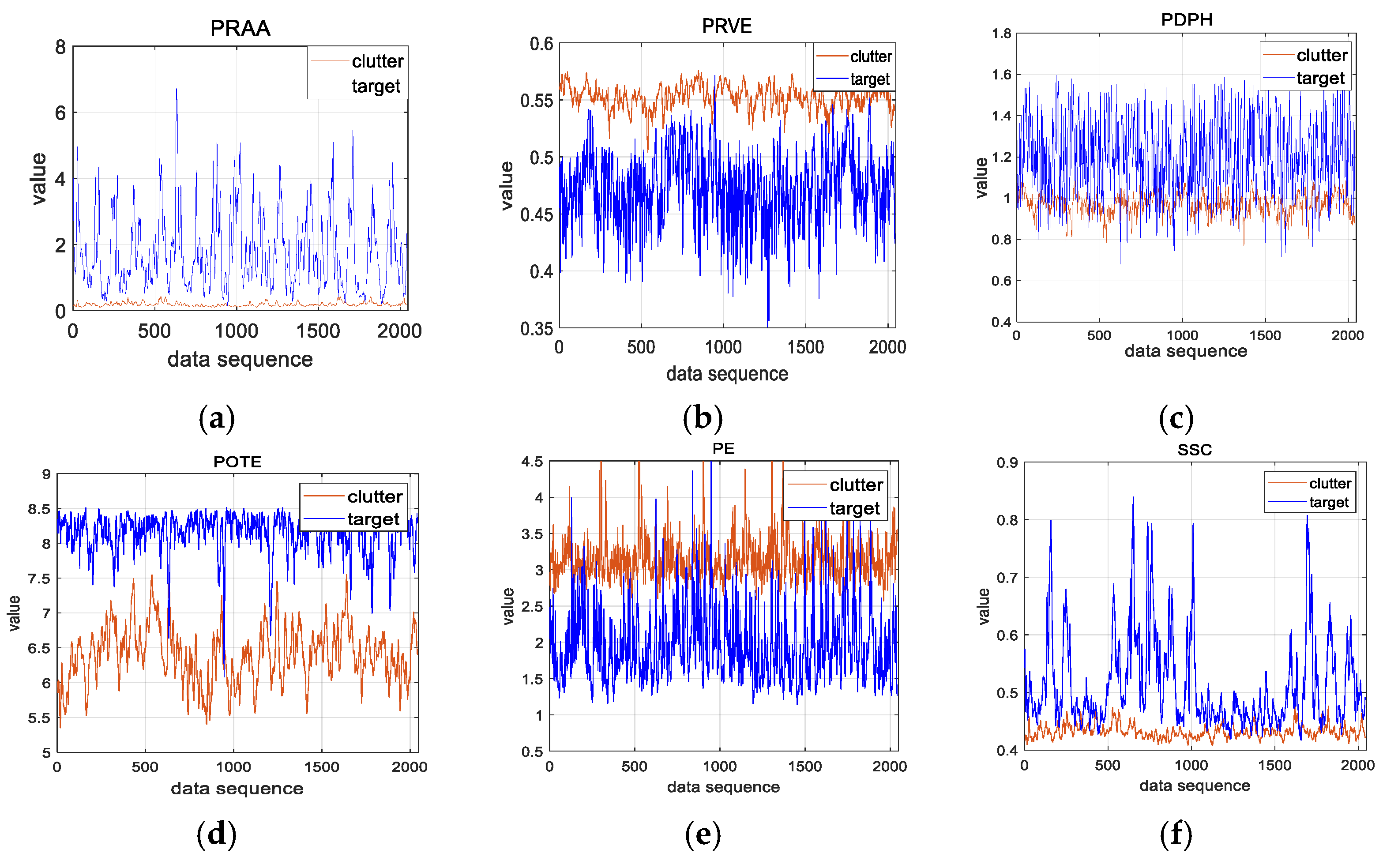
Firstly, we analyze the separability of the proposed features. Taking the dataset 54 as an example, with a sample size of 2000 and 512 sampling points per sample, we extracted the feature values of the target unit (distance unit 9) and the pure sea clutter unit (distance unit 1), respectively. The results are shown in Figure 5. From Figure 5, it can be seen that the PRAA, PDPH, POTE, and SSC values of the target are all higher than those of sea clutter. Among them, POTE has the best separability, followed by PRAA and SSC, and finally PDPH. The PRVE and PE values of pure sea clutter are higher than those of the target unit, consistent with their physical significance.

Secondly, to quantitatively assess the separability of features before and after fusion, a separability measurement function is defined to evaluate the features pre- and post-fusion. The definition of the separability measurement function is as follows [27]:

$$Z_S=trace\left({\displaystyle \frac{S_b}{S_w}}\right)$$

(26)

where trace represents trace operation, $S_b$ represents the inter-class scatter matrix of the sample, $S_w$ represents the intra-class scatter matrix, and the larger the value of $Z_S$, the better the separability of the sample.

Four IPIX datasets from 1993 were selected to validate the intra-domain network fusion effect employed in MP-FFN. The ASCR for dataset 54 was 11.95 dB, while for dataset 17, it was 13.88 dB. Additionally, the ASCR for dataset 280 was 6.20 dB, and for dataset 310, it was 2.62 dB. The results are presented in

Table 4. Separability measurement values before and after feature fusion at 128 ms.

Feature	17	54	280	310
PRAA	0.1446	0.8015	0.2717	0.1737
PRVE	0.2711	1.7218	0.3128	0.2208
PDPH	0.6513	1.8952	0.3975	0.6177
POTE	0.5815	4.5309	0.5457	0.1891
Direct splicing	1.3085	6.5120	0.9781	0.8557

for an observation time of 128 ms.

From Table 4, it is evident that for the same dataset and observation time, the separability metrics of PRAA and PRVE are relatively low, whereas the separability metrics of PDPH and POTE are relatively high. After direct concatenation, the analyzability metrics of the features were significantly improved. However, in the proposed method, the separability metrics of the fused features using SAE increase even more, approaching nearly twice the highest single-feature metric before concatenation. From this, it can be concluded that using SAE for feature fusion in the proposed MP-FFN domain network can effectively improve the separability of clutter and target samples.

Finally, the fusion of multiple-domain features ensures complementarity in feature detection across various scenarios, taking into account the impact of different feature domains on detection performance. The description of detection scenes is presented in

Table 5. Feature selection settings of six Detection scenes.

Settings	Number	Feature Selection	Feature Domain
Scene (1)	1	PRAA	Time
Scene (2)	1	PRVE	Frequency
Scene (3)	2	PRVE, PDPH	Frequency
Scene (4)	3	PRAA, PRVE, PDPH	Time and frequency
Scene (5)	4	PRAA, PRVE, PDPH, POTE	Time, frequency, and fractal
Scene (6)	6	PRAA, PRVE, PDPH, POTE, PE, SSC	Time, frequency, fractal, and polarization

.

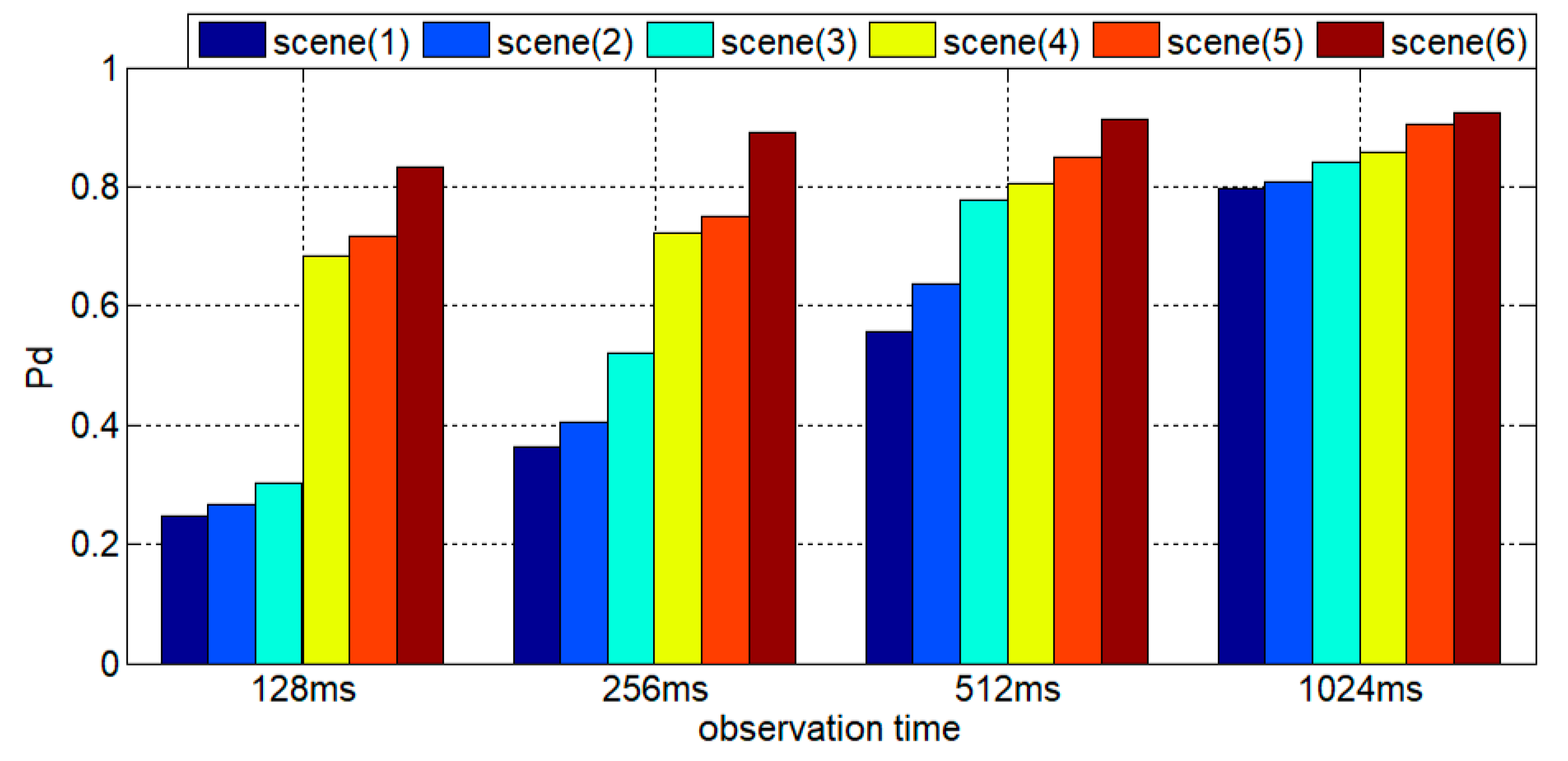
The performance of the proposed MP-FFN was validated by calculating the detection rate to evaluate the experimental results. Dataset 54 was selected, with observation times set to 128 ms, 256 ms, 512 ms, and 1024 ms, respectively, and a false alarm rate of 0.001 was maintained. The results are presented in

Table 6. Detection rate utilizing different features.

Observation Time	128 ms	256 ms	512 ms	1024 ms
Scene (1)	0.2466	0.3631	0.5557	0.7983
Scene (2)	0.2662	0.4059	0.6365	0.8081
Scene (3)	0.3028	0.5215	0.7772	0.8401
Scene (4)	0.6838	0.7237	0.8066	0.8573
Scene (5)	0.7155	0.7506	0.8494	0.9041
Scene (6)	0.8339	0.8900	0.9130	0.9250

.

To facilitate a better comparison of the experimental results, the detection rates are represented in the form of a histogram in Figure 6.

From Table 6, it is evident that employing a single time-domain feature (scene (1)) or frequency-domain feature (scene (2)) for detection purposes results in a lower detection rate due to the inherent limitations of these features. Specifically, at 128 ms and 256 ms, the detection rate drops below 50%. By fusing two frequency-domain features (scene (3)), a marginal improvement in detection rate is achieved, yet the detection rate remains low even at 128 ms. However, when the time-domain and frequency-domain feature domains are fused (scene (4)), a significant boost in detection rate is observed. By integrating the time domain, frequency domain, and fractal domain (scene (5)), the detection rate is further elevated. The proposed algorithm integrates four feature domains: time domain, frequency domain, fractal domain, and polarization domain (scene (6)), achieving the highest detection rate. Referring to Figure 6, it becomes apparent that within the same scene, the detection rate increases as observation time prolongs. Additionally, at a constant observation time, an increase in feature domains leads to a higher detection rate. From this, it can be inferred that expanding the feature domains can enhance detection performance.

4.3. Performance of the Proposed Method

The proposed method incorporates constraint-based optimization within the intra-domain network architecture to minimize feature redundancy. The selection of parameters also significantly impacts the fused network. We will elaborate on this issue from the following two aspects:

(1)

Impact of network constraints on algorithm performance

The MP-FFN proposed in this paper integrates features via an intra-domain network, which employs SAE for fusion. The objective is to minimize redundant information among features within the same domain while preserving as much separable information as possible. It reduces the feature dimensionality through an AE network, while simultaneously limiting information loss. Additionally, other constraints are employed to enhance the separability of the reduced-dimension features. The number of SAE layers in each feature domain is determined by the number of features; the more features there are in the domain, the more layers are used. The loss function utilized by the intra-domain network primarily consists of two components: the reconstruction loss $J_{reconstruction}^{domain}$, which is composed of the reconstruction term of SAE, and the proportional loss $J_{ratio}^{domain}$, which arises from the class-to-class and within-class ratio constraint. We analyze the following four situations:

Situation (1): MP-FFN without reconstruction loss $J_{reconstruction}^{domain}$. Compared to the baseline network method, an intra-class and inter-class ratio constraint was added. This situation served as a comparative experiment to validate the effectiveness of the intra-class and inter-class ratio.

Situation (2): MP-FFN without proportional loss $J_{ratio}^{domain}$. Compared to the baseline network method, an AE constraint was added. This situation was used as a comparative experiment to verify the effectiveness of AE.

Situation (3): MP-FFN without both $J_{reconstruction}^{domain}$ and $J_{ratio}^{domain}$. This situation employs MP-FFN after removing the AE constraint and the intra-class to inter-class ratio constraint. At this point, the network’s loss function solely comprises the cross-entropy and regularization term constraints from the inter-domain network.

Situation (4): MP-FFN, including AE constraint, intra-class and inter-class ratio constraint, cross-entropy, and regularization term constraint.

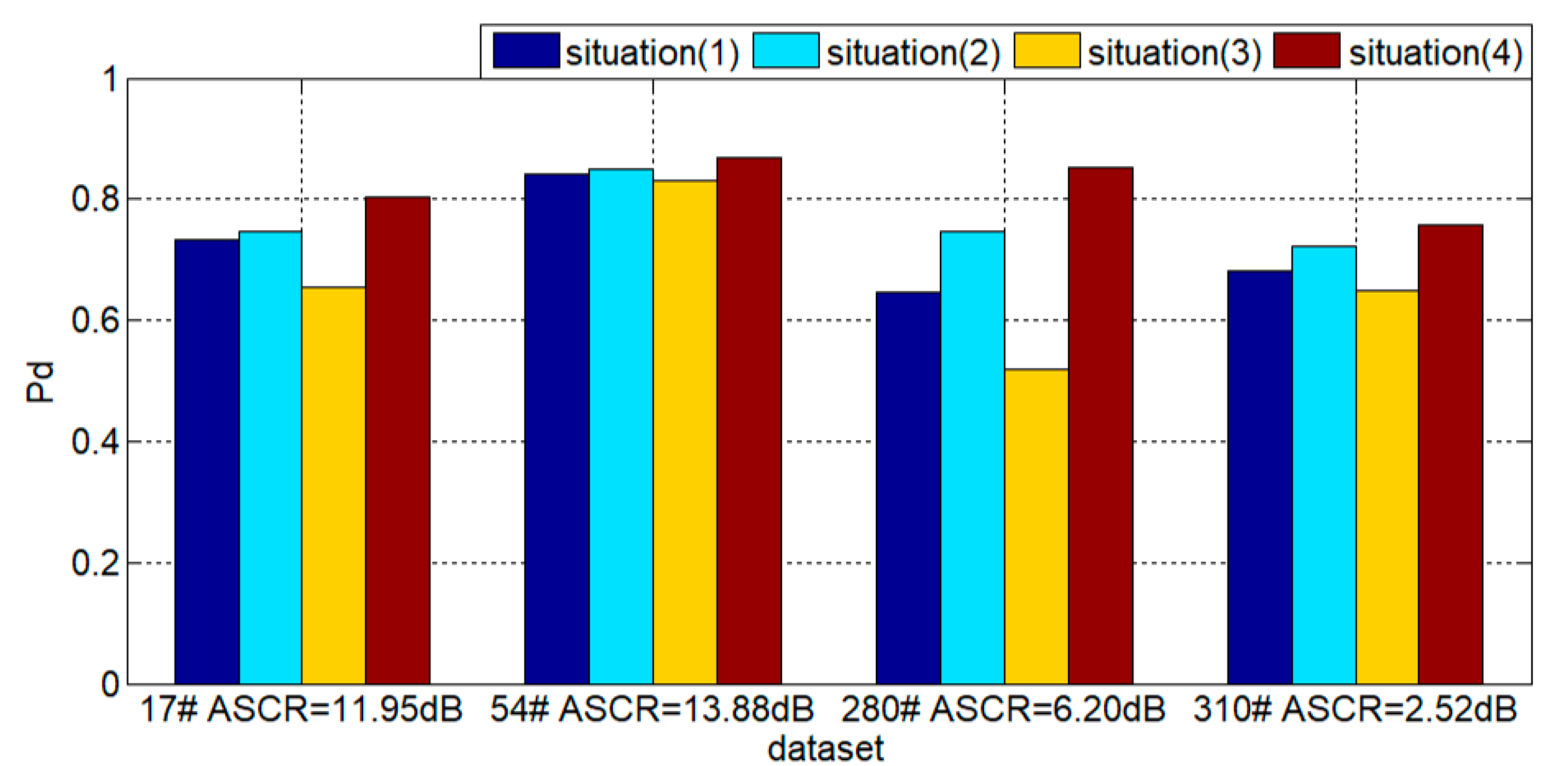
The datasets 17, 54, 280, and 310 were used to verify the above situations. The observation time was selected as 512 ms, and the results are shown in

Table 7. Detection rate in different constraint situations.

Settings	17	54	280	310
Situation (1)	0.7332	0.8421	0.6450	0.6818
Situation (2)	0.7479	0.8507	0.7479	0.7222
Situation (3)	0.6536	0.8311	0.5177	0.6499
Situation (4)	0.8042	0.8690	0.8519	0.7576

.

To quantitatively demonstrate the performance improvement achieved through constraint implementation, Figure 7 presents a comparative histogram analysis of the detection results documented in Table 7.

As evident from Table 7, when only the inter-domain network is employed to constrain the algorithm (situation (3)), the detection rate is the lowest across all four datasets; adding only the proportional loss (situation (1)) improves the detection rate to some extent; adding only the reconstruction loss (situation (2)) significantly boosts the detection rate; employing the complete MP-FFN (situation (4)) results in the greatest increase in detection rate. For dataset 54 with a higher ASCR, the algorithm with the complete network performs 3.79% better than without intra-domain network constraints. For dataset 280 with a lower ASCR, the algorithm with the complete network outperforms the network without intra-domain network constraints by 34.02%.

As shown in Figure 7, across the four datasets, the completed MP-FFN exhibits the highest detection rate, followed by the network with AE constraints added through reconstruction loss, and then the network with intra-class and inter-class constraints added through proportional loss. The detection rate is lowest when there are no intra-domain network constraints. This leads to the conclusion that MP-FFN, by adding AE constraints and intra-class and inter-class constraints through the intra-domain network, reduces redundancy between fused features while retaining their effective information, thereby enhancing detection performance.

(2)

The impact of network parameters on algorithm performance

We investigate the impact of four parameters on algorithm performance: the number of layers in the intra-domain network, the number of layers in the inter-domain network, as well as parameters $\alpha$ and $\beta$.

(1)

Discussion on the number of network layers

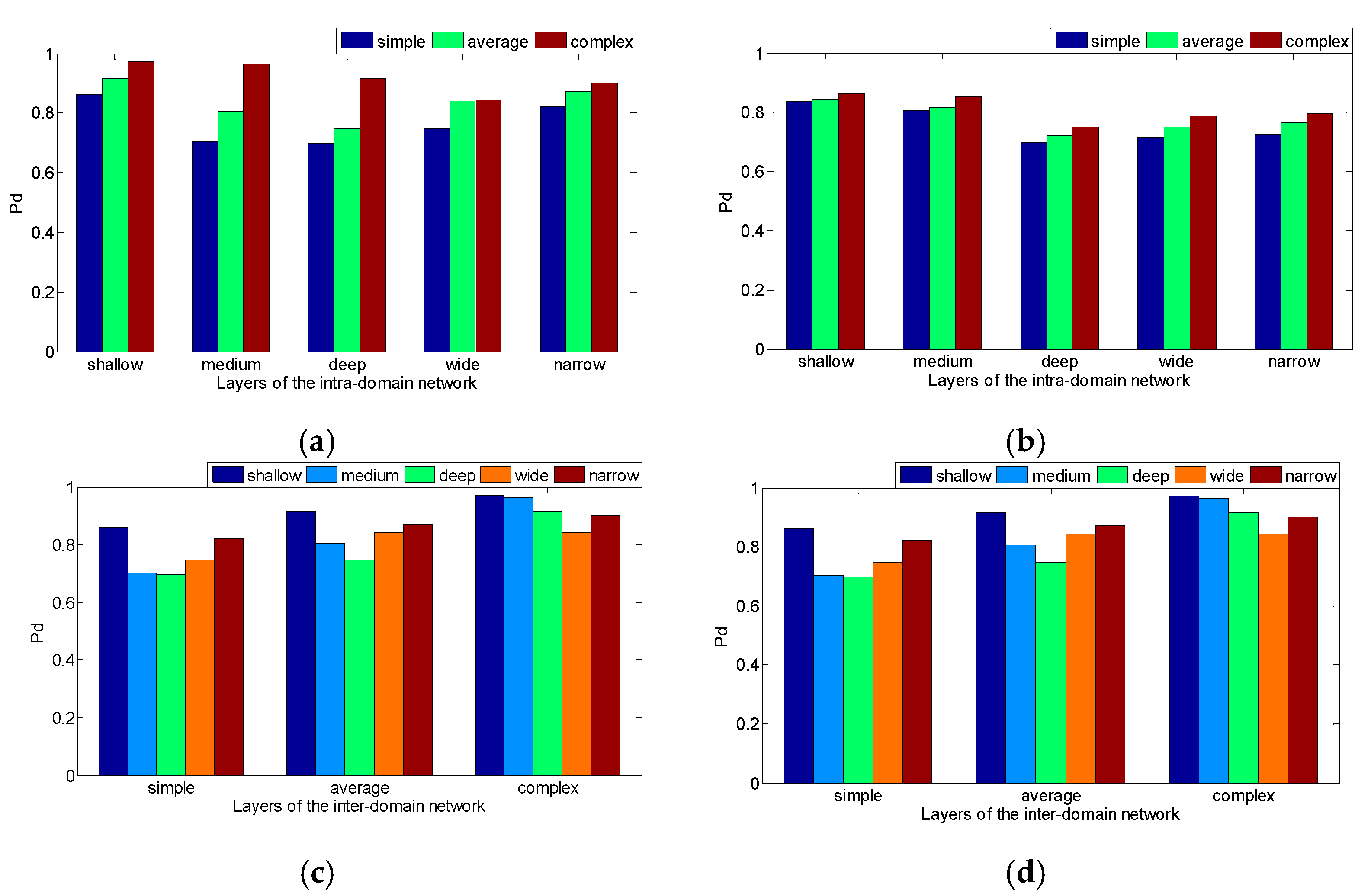
Experiments were conducted using dataset 54, with an observation time of 512 ms and a false alarm rate limited to 0.001. The parameter settings for the intra-domain network are outlined in

Table 8. SAE hidden layer settings.

Type	Number of Layers	Number of Neurons per Layer
Shallow	1	4
Medium	2	8, 4
Deep	3	16, 8, 4
Wide	1	16
Narrow	1	8

, while those for the inter-domain network are detailed in

Table 9. Inter-domain network layer settings.

Type	Number of Layers	Number of Neurons per Layer
Simple	1	8
Average	2	16,8
Complex	3	32,16,8

. Detection rates were calculated for various parameter configurations.

Take $\alpha =0.01$, $\beta =0.01$ and $\alpha =0.01$, $\beta =0.001$, respectively, and set different network layers. To more intuitively compare the results, we plotted the detection rates in the form of histograms, as illustrated in Figure 8. Specifically, the abscissa in Figure 8a,b represents the type of intra-domain network, while the abscissa in Figure 8c,d represents the type of inter-domain network. Figure 8a,c correspond to $\alpha =0.01$, $\beta =0.01$, whereas Figure 8b,d correspond to $\alpha =0.01$, $\beta =0.001$.

For intra-domain networks, Figure 8a,b demonstrate that the detection rate decreases as the number of layers increases. Regarding the number of neurons in a single layer, as the SAE type varies among “shallow”, “narrow”, and “wide”, the number of neurons in a single layer gradually increases, with average detection rates of 0.8828, 0.8136, and 0.7810, respectively, indicating a gradual decrease in detection performance. Based on these findings, it can be concluded that the shallow, low-dimensional SAE type is more effective.

For inter-domain networks, Figure 8c,d reveal that the detection rate shows an increasing trend as the number of layers increases. Therefore, it can be inferred that complex inter-domain networks contribute to enhancing detection performance.

(2)

Discussion on α and β

In MP-FFN, $\alpha$ and $\beta$ are utilized to adjust the weights of reconstruction loss and proportional loss within the intra-domain network loss function. The reconstruction loss facilitates the encoder in learning superior feature representations, thereby preventing the network from skewing toward incorrect classification tasks during training. Both intra-category and inter-category losses enhance category discrimination, allowing samples from the same category to be more concentrated, while samples from different categories become more dispersed. However, if $\alpha$ and $\beta$ are set to inappropriate values, it can easily lead to a mismatch in quantity sets during the learning process of the intra-domain network. Selecting an appropriate $\alpha$ is crucial for ensuring the stability of feature extraction and preventing model drift. Meanwhile, $\beta$ plays a role in guiding the model to learn more distinct feature representations while preserving the overall feature structure. By choosing suitable values for both $\alpha$ and $\beta$, we can jointly optimize the feature space, ultimately enhancing detection performance.

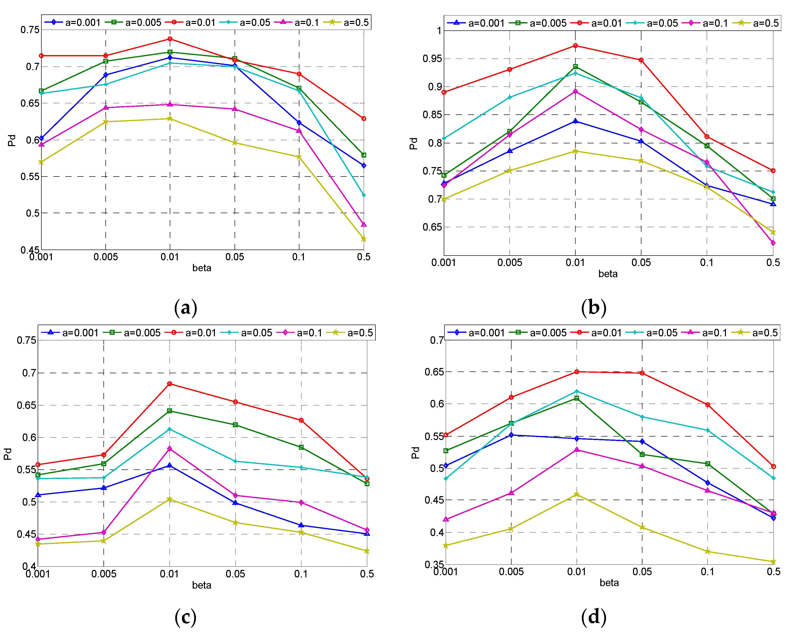
To quantify the influence of regularization parameters $\alpha$ and $\beta$, we performed comprehensive experiments on datasets 17, 54, 280, and 310 with varying parameter combinations. The observation time was set to 512 ms, the intra-domain network had one layer with four neurons, the inter-domain network was configured with three layers, and the false alarm rate was maintained at 0.001. The hyperparameters $\alpha$ and $\beta$ were systematically evaluated across a logarithmically scaled range: 0.001, 0.005, 0.01, 0.05, 0.1, and 0.5. The quantitative relationship between parameter variations $\left(\alpha ,\beta \right)$ and detection performance is shown in Figure 9.

The results presented in Figure 9 demonstrate that as $\alpha$ and $\beta$ increase, the detection rate first rises and then falls, peaking at 0.01. Notably, $\alpha$ and $\beta$ maintain a high detection rate when valued in the 10⁻² range. As $\alpha$ and $\beta$ decrease, detection performance declines. When these values are very small, the decline in detection performance becomes less pronounced. Conversely, as $\alpha$ and $\beta$ increase, detection performance also deteriorates, with a rapid decline in detection rate when values exceed 0.1. In summary, the hyperparameters $\alpha$ and $\beta$ should ideally be set in the 10⁻² range, avoiding excessively large values.

5. Discussion

5.1. Comparison of Different Detection Methods

We compare the proposed MP-FFN with both the classical sea surface target detection method and the feature detection methods based on multi-domain feature fusion proposed in recent years. The former calculates the detection rate of the method under a given false alarm rate, whereas the latter is a classification method with limited false alarm control capability.

(1)

Comparison with classical methods for sea surface target detection

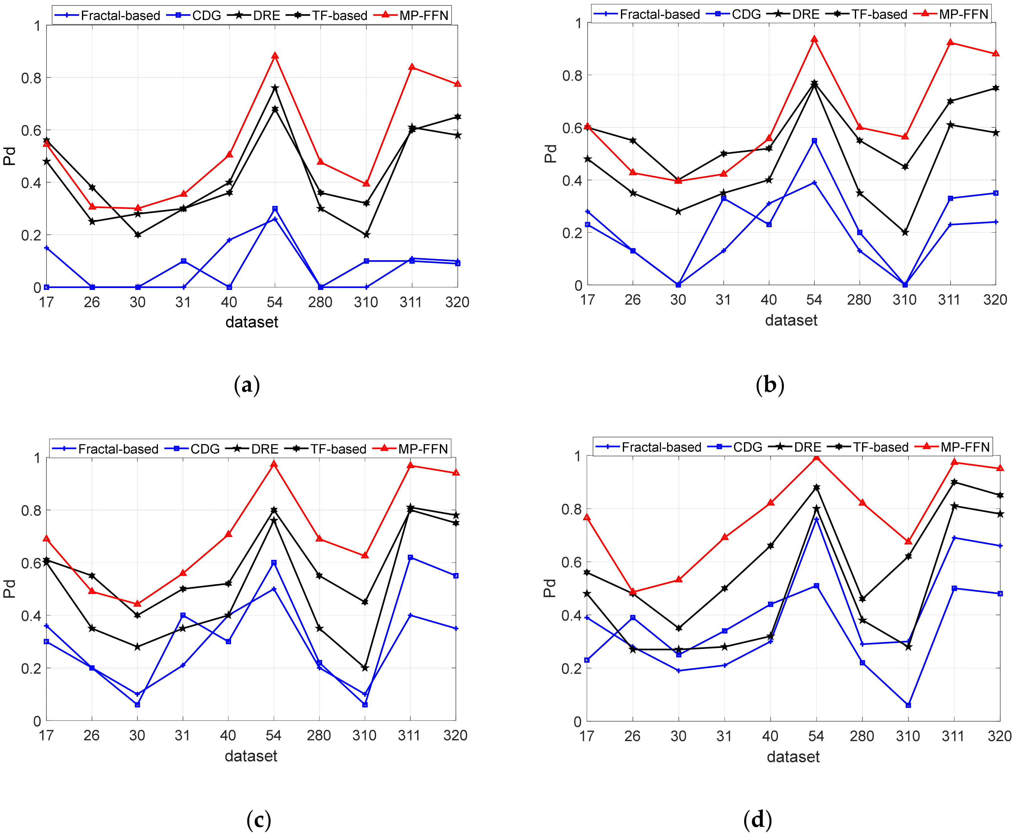
The proposed method, abbreviated as MP-FFN, was compared with existing fractal-based method [7], TF-based method [8], CDG method [9], and DRE method [10]. The results are shown in Figure 10, which shows the average detection rates of all methods on the ten datasets of IPIX with observation times of 128 ms, 256 ms, 512 ms, and 1024 ms, respectively, with false alarms controlled at 0.001.

From Figure 10, it can be seen that when the observation time is 128 ms, although the fractal-based method and CDG method are relatively simple, their detection performance is poor. The DRE method and three-feature method show certain detection effects compared to the proposed method, and the proposed method is slightly better than the other two methods with respect to the vast majority of datasets. From Figure 10b,c, it can be observed that as the observation time increases, the detection performance of all methods improves, with the proposed method and DRE method achieving the best detection performance. From Figure 10d, it can be seen that the proposed method has the best detection performance at 1024 ms.

5.2. Comparison of Different Detection Methods Based on Feature Fusion

To validate the effectiveness of the proposed MP-FFN in enhancing detection performance, we conducted experiments using En-OCSVM [18], CNN [20], Transformer [21], the MP-FFN without false alarm control and the complete MP-FFN on the six features presented in our method. Since En-OCSVM, CNN, and Transformer lack the ability to control false alarms, we employ the following approach to calculate the detection rate, false alarm rate, and accuracy rate:

$$P_d={\displaystyle \frac{N_{target}}{N_{total}}}$$

(27)

$$P_{fa}={\displaystyle \frac{N_{Fa}}{N_{Clutter}}}$$

(28)

$$C_R={\displaystyle \frac{N_{Correct}}{N_{total}}}$$

(29)

where $N_{Correct}$ represents the number of correctly classified samples in the test set, $N_{total}$ represents the total number of samples in the test set, $N_{Fa}$ represents the number of samples judged as targets for clutter, $N_{Clutter}$ represents the total number of test samples for clutter, and $N_{target}$ represents the total number of test samples for targets. The average results of 10 IPIX datasets, with observation times selected as 128 ms, 256 ms, 512 ms, and 1024 ms, respectively, are presented in

Table 10. Detection performance of different methods with an observation time of 128 ms.

Methods	Pd	Pfa	Cr
En-OCSVM [18]	0.4493	0.0544	0.8231
CNN [20]	0.4376	0.0053	0.9439
Transformer [21]	0.3576	0.0063	0.9372
MP-FFN without Pfa	0.5388	0.0026	0.9621
MP-FFN	0.5375	0.0010	0.9060

,

Table 11. Detection performance of different methods with an observation time of 256 ms.

Methods	Pd	Pfa	Cr
En-OCSVM [18]	0.5352	0.0567	0.8433
CNN [20]	0.5710	0.0062	0.9536
Transformer [21]	0.3850	0.0043	0.9416
MP-FFN without Pfa	0.6076	0.0025	0.9671
MP-FFN	0.6317	0.0010	0.9289

,

Table 12. Detection performance of different methods with an observation time of 512 ms.

Methods	Pd	Pfa	Cr
En-OCSVM [18]	0.6125	0.0537	0.8651
CNN [20]	0.6029	0.0041	0.9606
Transformer [21]	0.4323	0.0100	0.9412
MP-FFN without Pfa	0.6880	0.0037	0.9684
MP-FFN	0.7202	0.0010	0.9359

and

Table 13. Detection performance of different methods with an observation time of 1024 ms.

Methods	Pd	Pfa	Cr
En-OCSVM [18]	0.6664	0.0528	0.8788
CNN [20]	0.6409	0.0090	0.9617
Transformer [21]	0.3473	0.0078	0.9355
MP-FFN without Pfa	0.7755	0.0030	0.9746
MP-FFN	0.7807	0.0010	0.9541

.

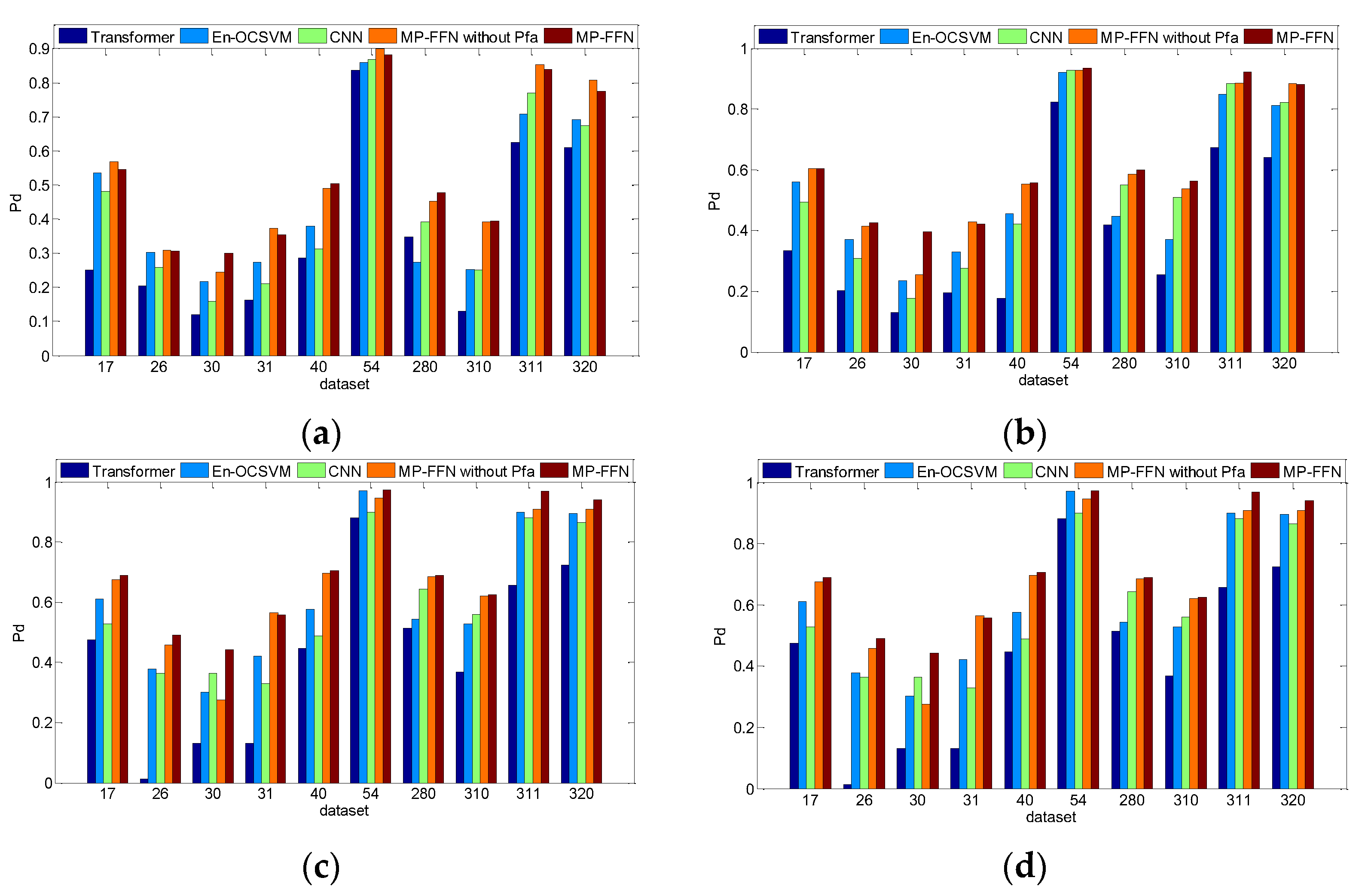
To better illustrate the detection effectiveness, we have displayed the results of each set of data in the form of a histogram, as illustrated in Figure 11.

From Table 10, Table 11, Table 12 and Table 13, it is evident that under the same observation time and when using the same features for detection, MP-FFN exhibits the highest detection rate and accuracy while stably maintaining a false alarm rate of 0.001. The detection rate using CNN is slightly higher than that using En-OCSVM, except at 256 ms, where the detection rate using En-OCSVM is slightly higher than that using CNN; however, CNN has a lower false alarm rate. Lastly, the Transformer method, despite having a false alarm rate below 0.01, has a detection rate at least 8% lower than the other three methods. As Figure 11 shows, with increasing observation time, the detection rate of most methods increases. However, the Transformer method shows less improvement or even a decrease, while the proposed MP-FFN maintains the highest detection rate across all observation times.

It is worth noting that removing false alarm control may slightly improve the detection rate and accuracy in MP-FFN, but it is accompanied by an increase in the false alarm rate. In sea surface target detection, the detection rate must be based on the assumption that the false alarm rate is determined and remains unchanged. The complete MP-FFN can stably control the false alarm rate at 0.001, thus offering greater application value.

5.3. Stability of the Proposed Method

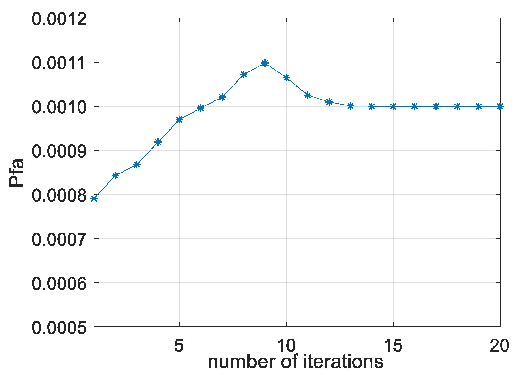
Finally, we analyze the stability of the proposed method using dataset 54 as an example. We utilize the first half of the data for training and the second half for testing. Setting the iteration count to 20, we record the variations in false alarm rate, detection rate, and accuracy rate, as illustrated in Figure 12. As evident from Figure 12, as the iteration count increases, the false alarm rate initially rises and then gradually declines, stabilizing after nine iterations.

6. Conclusions

This paper proposes a maritime target detection method using a hierarchical fusion network designed for weak signals and controllable false alarm rates. The approach begins by extracting six distinct features from radar echoes, leveraging full polarimetric information across time, frequency, fractal, and polarization domains. Features originating from the same domain are initially fused by an intra-domain network designed to minimize redundancy. Subsequently, an inter-domain network integrates the outputs from the different intra-domain networks. This hierarchical architecture leverages the complementary nature of multi-domain features to enhance separability, while optimized loss functions facilitate precise false alarm control. Verification on the IPIX dataset demonstrates that this method exhibits superior detection performance compared to traditional feature fusion techniques, primarily manifested in the following three aspects:

• The MP-FFN extracts six features from four distinct feature domains, adopting a full polarization perspective. Given the significant variations of different features and feature domains across various datasets, the detection effectiveness of the proposed method can be enhanced by at least 10% under different SCRs when compared to existing three-feature methods, methods based on time–frequency-domain features, and methods based on polarization-domain features;
• In MP-FFN, the intra-domain network minimizes feature redundancy and bolsters feature separability by computing intra-class and inter-class distances. Experimental results indicate a notable enhancement in feature separability after SAE fusion;
• The inter-domain network in the proposed method incorporates a dynamic threshold adjustment mechanism based on output probability ranking. By sorting the output results of the inter-domain network and setting an adaptive decision threshold, the detection performance can be improved by 10% compared to existing fusion algorithms, while satisfying the specified false alarm rate.

In conclusion, the proposed method exhibits excellent detection performance in scenarios involving weak target detection at sea. Since this method is based on feature-driven anomaly detection, encompassing feature extraction and classification between targets and clutter, the introduced MP-FFN is also suitable for applications such as target recognition and SAR image detection. However, a primary challenge of this method lies in the numerous hyperparameters of MP-FFN. The parameter tuning process consumes considerable time during the network model design and subsequent experimental stages. Integrating MP-FFN with an automatic tuning process to minimize human intervention and enhance model automation is the next step. Addressing this issue will facilitate the practical application of our method under various sea conditions. Additionally, given the complexity and variability of sea surface detection scenarios, selecting physically descriptive and refined features, as well as utilizing more extensive measured datasets for validation, are key focuses of our future research. This will pave the way for detecting smaller targets and maneuvering targets on the sea surface.

References

1. He, Y.; Huang, Y.; Guan, J.; Liu, N. Research progress in radar maritime target detection technology. J. Signal Process. 2025, 41, 969–992. [Google Scholar]
2. Guan, J. Summary of marine radar target characteristics. J. Radars 2020, 9, 674–683. [Google Scholar] [CrossRef]
3. Xu, S.; Bai, X.; Guo, Z.; Shui, P. Status and prospects of feature-based detection methods for floating targets on the sea surface. J. Radars 2020, 9, 684–714. [Google Scholar] [CrossRef]
4. Shi, Y.; Xie, X.; Li, D. Range distributed floating target detection in sea clutter via feature-based detector. IEEE Geosci. Remote Sens. Lett. 2016, 13, 1847–1850. [Google Scholar] [CrossRef]
5. Wang, Z.; Xin, Z.; Liao, G.; Huang, P.; Xuan, J.; Sun, Y.; Tai, Y. Land-sea target detection and recognition in SAR image based on non-local channel attention network. IEEE Trans. Geosci. Remote Sensing 2022, 60, 1–16. [Google Scholar] [CrossRef]
6. Fan, Y.; Wang, X.; Chen, S.; Guo, Z.; Su, J.; Tao, M.; Wang, L. Sea Surface Weak Target Detection Based on Weighted Difference Visibility Graph. IEEE Geosci. Remote Sens. Lett. 2025, 22, 3503605. [Google Scholar] [CrossRef]
7. Fan, Y.; Luo, F.; Li, M.; Hu, C.; Chen, S. Fractal properties of autoregressive spectrum and its application on weak target detection. IET Radar Sonar Navig. 2015, 9, 1070–1077. [Google Scholar] [CrossRef]
8. Shui, P.; Li, D.; Xu, S. Tri-Feature-Based Detection of Floating Small Targets in Sea Clutter. IEEE Trans. Aerosp. Electron. Syst. 2014, 50, 1416–1430. [Google Scholar] [CrossRef]
9. Yan, K.; Wu, H.; Xiao, H.; Zhang, X. Novel robust band-limited signal detection approach using graphs. IEEE Commun. Lett. 2017, 21, 20–23. [Google Scholar] [CrossRef]
10. Shi, S.; Jiang, L.; Cao, D.; Zhang, Y. Sea-surface small target detection using entropy features with dual-domain clutter suppression. Remote Sens. Lett. 2022, 13, 1142–1152. [Google Scholar] [CrossRef]
11. Shi, S.; Zhang, R.; Wang, J.; Li, T. Dual-Channel Detection of Sea-Surface Small Targets in Recurrence Plot. IEEE Geosci. Remote Sens. Lett. 2025, 22, 3503005. [Google Scholar] [CrossRef]
12. Gu, T. Detection of Small Floating Targets on the Sea Surface Based on Multi-Features and Principal Component Analysis. IEEE Geosci. Remote Sens. Lett. 2020, 17, 809–813. [Google Scholar] [CrossRef]
13. Ruff, L.; Vandermeulen, R.; Goernitz, N.; Deecke, L.; Siddiqui, S.A.; Binder, A.; Müller, E.; Kloft, M. Deep One-Class Classification. In Proceedings of the International Conference on Machine Learning, Stockholm, Sweden, 10–15 July 2018. [Google Scholar]
14. Zhang, X.; Li, P.; Cai, C. Regional Urban Extent Extraction Using Multi-Sensor Data and One-Class Classification. Remote Sens. 2015, 7, 7671–7694. [Google Scholar] [CrossRef]
15. Maaten, L.; Hinton, G. Visualizing Data Using T-SNE. J. Mach. Learn. Res. 2008, 9, 2579–2605. [Google Scholar]
16. Villeval, S.; Bilik, I.; Gürbuz, S.Z. Application of a 24 GHz FMCW Automotive Radar for Urban Target Classification. In Proceedings of the 2014 IEEE Radar Conference, Cincinnati, OH, USA, 19–23 May 2014. [Google Scholar]
17. Chen, S.; Luo, F.; Luo, X. Multi-view Feature-based Sea Surface Small Target Detection in Short Observation Time. IEEE Geosci. Remote Sens. Lett. 2021, 18, 1189–1193. [Google Scholar] [CrossRef]
18. Chen, S.; Ouyang, X.; Luo, F. Ensemble One-class Support Vector Machine for Sea Surface Target Detection Based on K-means Clustering. Remote Sens. 2024, 16, 2401. [Google Scholar] [CrossRef]
19. Wang, Z.; Hou, G.; Xin, Z.; Liao, G.; Huang, P.; Tai, Y. Detection of SAR image multiscale ship targets in complex inshore scenes based on improved YOLOv5. IEEE J. Sel. Top. Appl. Earth Obs. Remote Sens. 2024, 17, 5804–5823. [Google Scholar] [CrossRef]
20. Shi, Y.; Tao, P.; Xu, S. Small float target detection in sea clutter based on WGAN-GP-CNN. Signal Process. 2024, 40, 1082–1097. [Google Scholar]
21. Chen, K.; Liu, X.; Shen, C. Transformer-based Radar/Lidar/Camera Fusion Solution for 3D Object Detection. Flight Control Detect. 2025, 8, 82–92. [Google Scholar]
22. Shi, S.; Shui, P. Sea-surface Floating small target detection by one-class classifier in time-frequency feature space. IEEE Trans. Geosci. Remote Sens. 2018, 56, 6395–6411. [Google Scholar] [CrossRef]
23. Anderson, S.J.; Morris, J.T. Aspect Dependence of the Polarimetric Characteristics of Sea Clutter: II. Variation with Azimuth Angle. In Proceedings of the 2008 International Conference on Radar, Adelaide, SA, Australia, 2–5 September 2008. [Google Scholar]
24. An, W.; Cui, Y.; Zhang, W.; Yang, J. Data Compression for Multilook Polarimetric SAR Data. IEEE Geosci. Remote Sens. Lett. 2009, 6, 476–480. [Google Scholar] [CrossRef]
25. An, W.; Cui, Y.; Yang, J. Three-Component Model-Based Decomposition for Polarimetric SAR Data. IEEE Trans. Geosci. Remote Sens. 2010, 48, 2732–2739. [Google Scholar] [CrossRef]
26. Gao, Y.; Zhou, Y.; Wang, Y.; Zhuo, Z. Narrowband Radar Automatic Target Recognition Based on a Hierarchical Fusing Network with Multidomain Features. IEEE Geosci. Remote Sens. Lett. 2021, 18, 1039–1043. [Google Scholar] [CrossRef]
27. Zhang, W.; Du, L.; Li, L.; Zhang, X.; Liu, H. Infinite Bayesian One-Class Support Vector Machine Based on Dirichlet Process Mixture Clustering. Pattern Recognit. 2018, 78, 56–78. [Google Scholar] [CrossRef]
Figure 1. The specific process of the proposed detector.
Remotesensing 17 03213 g001
Figure 2. Intra-domain network based on SAE. The hidden layer features of the intra-domain network are used as input to the inter-domain networks.
Remotesensing 17 03213 g002
Figure 3. Inter-domain network based on MLPs.
Remotesensing 17 03213 g003
Figure 4. Flowchart for controlling the false alarm rate of the detection network.
Remotesensing 17 03213 g004
Figure 5. Feature extraction from four different domains of target and clutter in the IPIX dataset. (a) PRAA; (b) PRVE; (c) PDPH; (d) POTE; (e) PE; and (f) SSC.
Remotesensing 17 03213 g005
Figure 6. Detection rates of MP-FFN under six different scenarios.
Remotesensing 17 03213 g006
Figure 7. Detection performance among different datasets.
Remotesensing 17 03213 g007
Figure 8. Impact of network type on detection performance. (a) Detection rate for changes in inter-domain network types when α = 0.01 , β = 0.01 ; (b) Detection rate for changes in inter-domain network types when α = 0.01 , β = 0.001 ; (c) Detection rate for changes in intra-domain network types when α = 0.01 , β = 0.01 ; (d) Detection rate for changes in intra-domain network types when α = 0.01 , β = 0.001 .
Remotesensing 17 03213 g008
Figure 9. Detection rates of MP-FFN when different parameters are selected: (a) dataset 17; (b) dataset 54; (c) dataset 280; and (d) dataset 310.
Remotesensing 17 03213 g009
Figure 10. Feature extraction from four different domains of target and clutter in the IPIX dataset: (a) 128 ms; (b) 256 ms; (c) 512 ms; and (d) 1024 ms.
Remotesensing 17 03213 g010
Figure 11. Detection rates of different methods on 10 datasets at different observation times: (a) 128 ms; (b) 256 ms; (c) 512 ms; and (d) 1024 ms.
Remotesensing 17 03213 g011
Figure 12. False alarm rate of the hierarchical fusion network at 20 iterations.
Remotesensing 17 03213 g012