Article

Dynamic Landslide Susceptibility Assessment in the Yalong River Alpine Gorge Region Integrating InSAR-Derived Deformation Velocity

1
The College of Earth and Planet Science, Chengdu University of Technology, Chengdu 610059, China
2
The State Key Laboratory of Geohazard Prevention and Geoenvironment Protection, Chengdu University of Technology, Chengdu 610059, China
*
Author to whom correspondence should be addressed.
Remote Sens. 2025, 17(18), 3210; https://doi.org/10.3390/rs17183210
Submission received: 4 August 2025 / Revised: 1 September 2025 / Accepted: 12 September 2025 / Published: 17 September 2025
(This article belongs to the Special Issue Role of SAR/InSAR Techniques in Investigating Ground Deformation)

Abstract

Highlights

What are the main findings?
  • Quantifies deformation velocity as the second critical susceptibility factor (q = 0.21), enhancing spatial risk clustering characterization.
  • Achieves significant predictive gains (AUC = 0.9798, Kappa = 0.8870, 87.01% high-risk capture rate).
What is the implication of the main findings?
  • Provides a real-time early warning tool for landslides in high-risk terrains.
  • Validates deformation velocity as a measurable indicator for prioritizing geotechnical interventions.

Abstract

Dynamic susceptibility assessment is essential for mitigating evolving landslide risks in alpine gorge regions. To address the static limitations and unit mismatch issues in conventional landslide susceptibility assessments in alpine gorge regions, this study proposes a dynamic framework integrating time-series InSAR-derived deformation. Applied to the Xinlong–Kangding section of the Yalong River, annual surface deformation velocities were retrieved using SBAS-InSAR with Sentinel-1 data, identifying 24 active landslide zones (>25 mm/a). The Geodetector model quantified the spatial influence of 18 conditioning factors, highlighting deformation velocity as the second most significant (q = 0.21), following soil type. Incorporating historical landslide data and InSAR deformation zones, slope unit delineation was optimized to construct a refined sample dataset. A Random Forest model was then used to assess the contribution of deformation factors. Results show that integrating InSAR data substantially improved model performance: “Very High” risk landslides increased from 67.21% to 87.01%, the AUC score improved from 0.9530 to 0.9798, and the Kappa coefficient increased from 0.7316 to 0.8870. These results demonstrate the value of InSAR-based dynamic monitoring in enhancing landslide susceptibility mapping, particularly for spatial clustering, classification precision, and model robustness. This approach offers a more efficient dynamic evaluation pathway for dynamic assessment and early warning of landslide hazards in mountainous regions.

1. Introduction

Landslides represent one of the most widespread and destructive geological hazards globally [1,2], with amplified risks in alpine gorge regions. A representative region along the eastern Tibetan Plateau margin [3] demonstrates such vulnerability, where continuous uplift since the Late Cenozoic has formed gorges with relief >1000 m [4]. Compounding factors, including intense precipitation events [5,6,7], seismic activity, and anthropogenic engineering disturbances [8], further exacerbate slope instability. Consequently, landslides in these environments typically exhibit high suddenness (with average sliding velocities ranging from 10 to 30 m/s) [9], large scale (individual events exceeding tens of millions of cubic meters) [10], and pronounced cascading effects [11]. For instance, within the Yalong River Basin, the 2018 Baige landslide (~30 million m3) dammed the Jinsha River, necessitating the emergency evacuation of over 100,000 downstream residents [12]. Similarly, the 2020 Zhonghai Village landslide caused direct economic losses exceeding 200 million CNY [13], underscoring the severe threat these disasters pose to lifeline infrastructure and human settlements in this high-risk region.
Conventional landslide susceptibility assessment models primarily focus on static predisposing factors such as topography, geological structure, hydrological conditions, anthropogenic activities, and environmental variables [14,15,16,17,18,19,20,21,22,23,24,25,26]. Although essential, these static indicators are inherently unable to capture the dynamic processes driving landslide evolution [27]. This limitation becomes particularly critical in alpine gorge regions like the Yalong River Basin, where frequent rainfall events and seismic disturbances frequently induce significant surface deformation and deep-seated slope landslides [28,29]. Consequently, reliance solely on conventional static factors risks underestimating active landslide processes and fundamentally compromises the characterization of dynamic deformation responses to rainfall, seismic activity, and other external triggers [30,31,32,33,34].
To overcome the limitations of traditional landslide susceptibility assessment (LSA) methods, recent studies have introduced dynamic approaches that incorporate temporal variations in causal factors, rolling model updates, and multi-source data fusion. Among these, meteorologically driven models are the most common, using rainfall indicators within sliding time windows alongside terrain data for real-time shallow landslide prediction [35]. Typical dynamic variables include rainfall [36], seismic activity, vegetation disturbance [37], and freeze–thaw frequency [38], often integrated through temporal databases, time windows, and weighting schemes to enhance model adaptability [39]. However, these methods primarily rely on indirect environmental signals and lack direct observation of surface deformation processes.
In this context, Interferometric Synthetic Aperture Radar (InSAR) has emerged as a key tool for dynamic LSA, offering millimeter-level deformation accuracy and multi-temporal coverage [40,41,42]. With technological advances, InSAR has evolved from a post-event validation tool to a core component of susceptibility modeling, enabling the shift from static mapping to dynamic simulation [43,44]. Recent studies have explored its integration into LSA frameworks [45,46,47]. For instance, Chen et al. (2023) [48] and Zhu et al. (2025) [49] enhanced deformation datasets and applied dynamic weighting; Dai et al. (2023) [50,51] and Zhou et al. (2025) [52] combined InSAR with slope units to construct deformation–hazard matrices; Li et al. (2024) [53] and Wang et al. (2024) [54] achieved higher accuracy in cold regions by integrating multi-track deformation with machine learning models.
However, most existing studies still regard InSAR data primarily as an auxiliary or validation tool, which can only assess the partial accuracy of static susceptibility models. Few have systematically integrated InSAR-derived deformation metrics as independent predictive features within machine learning frameworks. More critically, the quantitative contribution of InSAR-based factors to model performance improvement remains largely unexplored, and the mechanisms by which their spatiotemporal heterogeneity influences the spatial variability of landslide susceptibility have not been adequately investigated. This research gap significantly limits the application potential of deformation-derived indicators in dynamic hazard susceptibility assessment.
In response to the above limitations, this study proposes a dynamic landslide susceptibility framework that integrates SBAS-InSAR-derived deformation velocity, geographical detector-based interaction analysis, and optimized slope unit partitioning. Focusing on a typical landslide-prone area in the middle and lower reaches of the Yalong River, annual deformation velocity fields (2020–2023) were extracted from ascending Sentinel-1 imagery. These were incorporated into a multi-source model alongside conventional static predictors. A Random Forest model was then applied to quantify the predictive value of deformation features, supported by SHAP (SHapley Additive exPlanations) interpretation and geographical interaction analysis, providing insights into the compound triggering mechanisms of landslides in complex alpine environments.

2. Study Area and Datasets

2.1. Study Area

The Yalong River (97°30′E–102°00′E, 28°00′N–33°30′N) traverses the eastern margin of the Tibetan Plateau, delineating a major north–south drainage system within the Hengduan Mountains. Its hydrological regime is governed by pronounced seasonal variability, primarily driven by the Indian Summer Monsoon and high-altitude glacial/snowmelt contributions. Prolonged tectonic uplift since the Late Cenozoic, driven by the continued convergence of the Indian and Eurasian plates, has shaped a deeply incised alpine gorge landscape dominated by steep “V”-shaped valleys. Tectonic uplift and fluvial incision rates in the central Himalayan gorges are generally estimated to range from 2 to 12 mm/a, with locally higher values up to 10 mm/a in active zones [55]. These intrinsic crustal dynamics, compounded by intensive dam and reservoir engineering, render the region particularly susceptible to geological hazards such as landslides and debris flows.
This study focuses on the Xinlong–Kangding reach in the upper gorge section of the Yalong River, as Figure 1, a 170 km segment within a 5660 km2 drainage area in southwestern Sichuan Province. Located in the transitional zone between the Songpan–Ganzi Fold Belt and the Xianshuihe Fault Zone, this area lies along the eastern front of the Tibetan Plateau. Characterized by high geological hazard exposure, densely populated valleys along transportation corridors, and intensive infrastructure development, the region calls for an urgent landslide susceptibility assessment to support evidence-based disaster risk reduction.

2.2. InSAR Data Sources

This study employed a series of Sentinel-1 C-band SAR Single Look Complex (SLC) data, which were freely obtained from the Alaska Satellite Facility (ASF) Vertex platform https://search.asf.alaska.edu (accessed on 8 February 2025). The LOS displacement time series across the study area were subsequently generated using Interferometric SAR (InSAR) techniques. All key sensor parameters are detailed in Table 1.
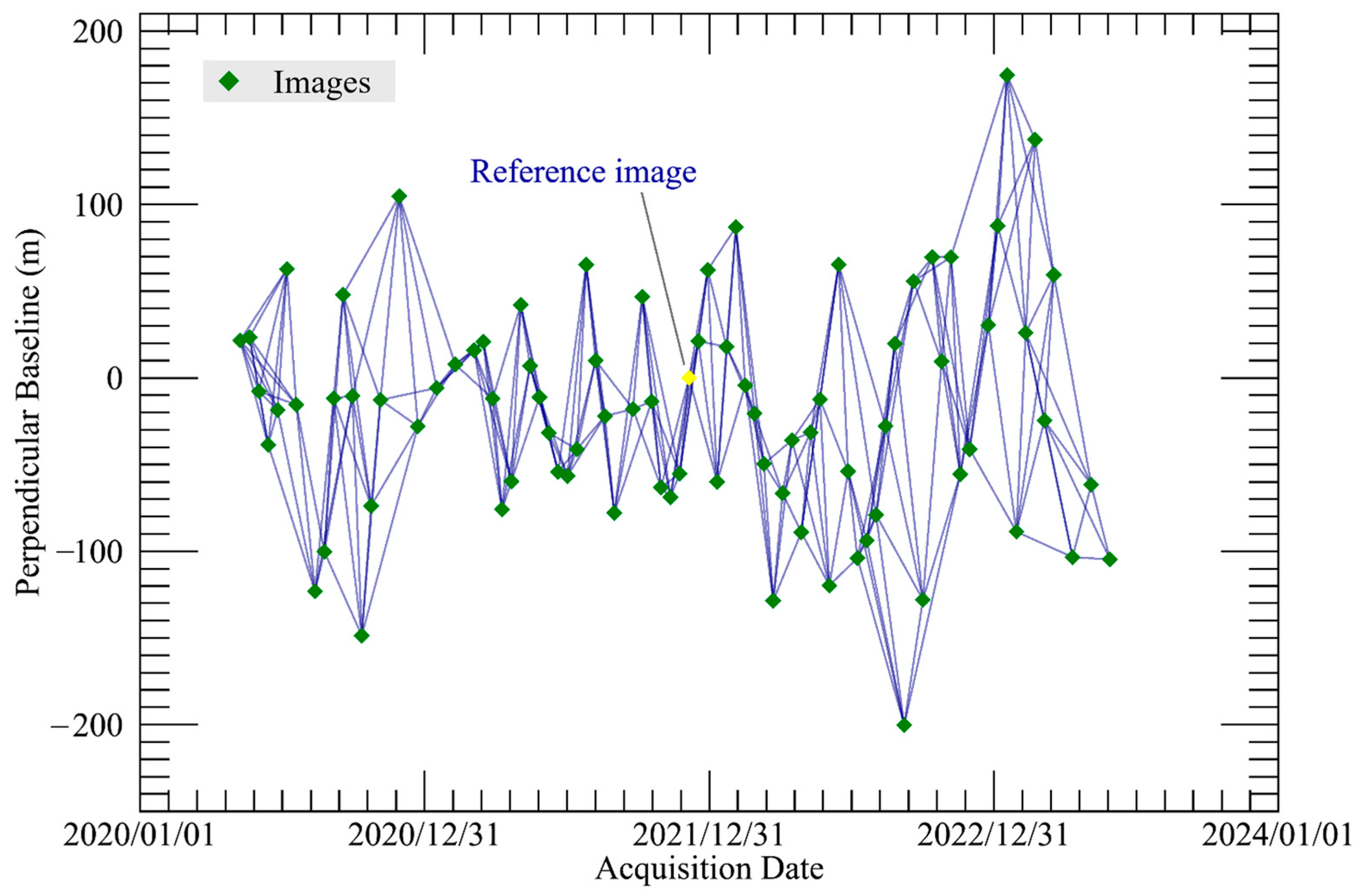
During interferometric processing, temporal and spatial baselines were constrained to ≤90 days and 160 m, respectively. Figure 2 illustrates the spatial–temporal baseline distribution of the interferometric pairs.

2.3. Landslide Conditioning Factors

Landslides result from the coupling of natural processes and anthropogenic activities, with occurrence mechanisms constrained by topography, hydrometeorological conditions, geological structures, land cover, and human disturbances. Establishing a multi-source indicator framework capturing both landslide preconditioning and triggering mechanisms is therefore essential for reliable susceptibility assessment.
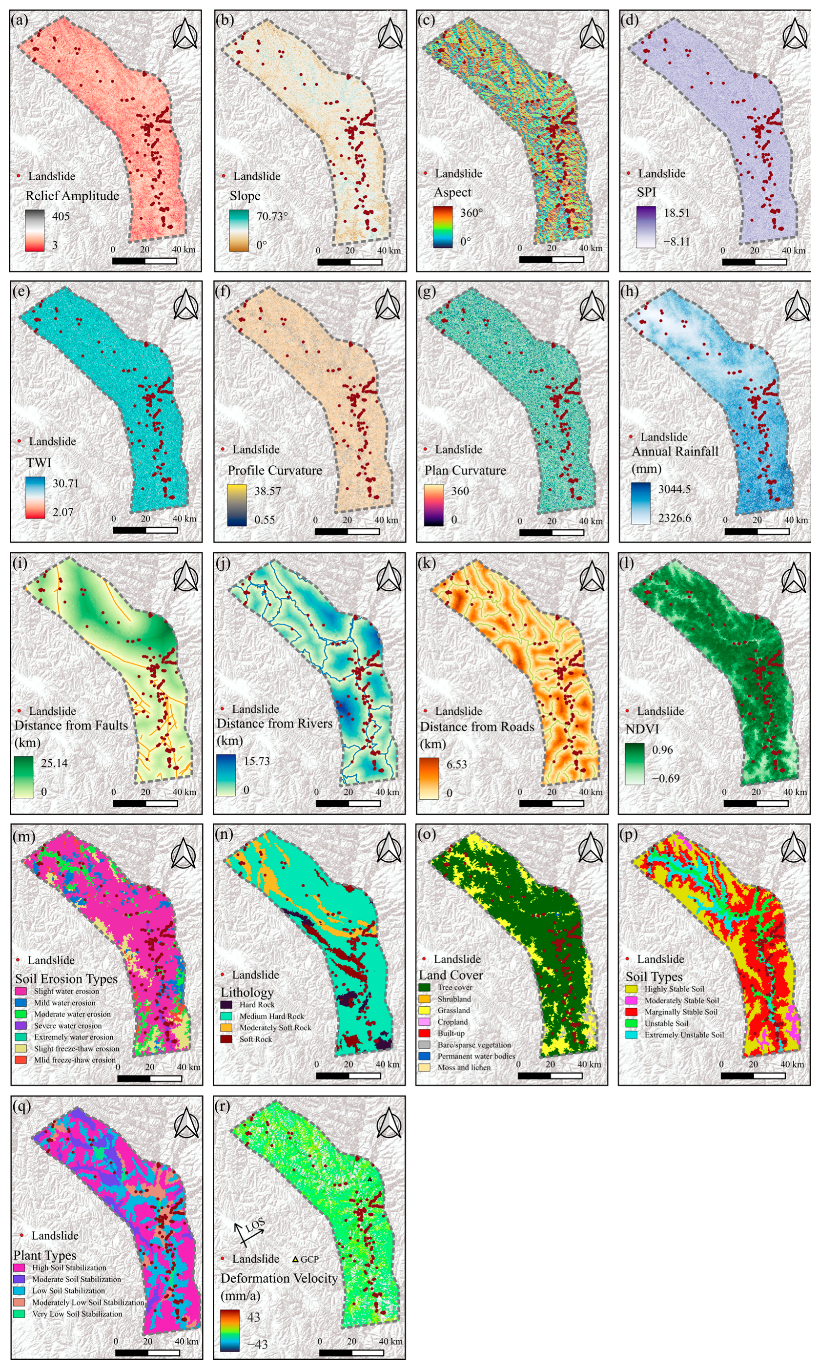
Building on prior research and regional landslide characteristics, this study selected 18 evaluation factors (Table 2, Figure 3) categorized into five groups:
  • Topographic Factors: Slope, Aspect, Relief Amplitude, Plan Curvature, and Profile Curvature. These factors govern overland flow convergence, mass wasting potential, and gravitational stress accumulation, exerting direct control over the spatial distribution of landslides.
  • Hydrometeorological Factors: Annual Precipitation, Stream Power Index (SPI), Topographic Wetness Index (TWI), and Distance from Rivers. These capture hydrodynamic processes and represent primary external triggers, particularly for rainfall-induced failures.
  • Plant and Soil Factors: Normalized Difference Vegetation Index (NDVI), Plant Types, Soil Types, and Soil Erosion Types. These modulate surface stability through runoff/erosion control and critically influence shallow landslide potential.
  • Geological Factors: Lithology and Distance from Faults. These determine rock/soil strength characteristics and structural fragmentation, constituting intrinsic controls on material stability.
  • Engineering Disturbance and Surface Deformation: Land Cover, Distance from Roads, and SBAS-InSAR-derived Deformation Velocity. Anthropogenic slope modifications such as road construction and excavation can induce mechanical instability, while surface deformation monitoring facilitates early identification of active or incipient slope failures.

3. Methodology

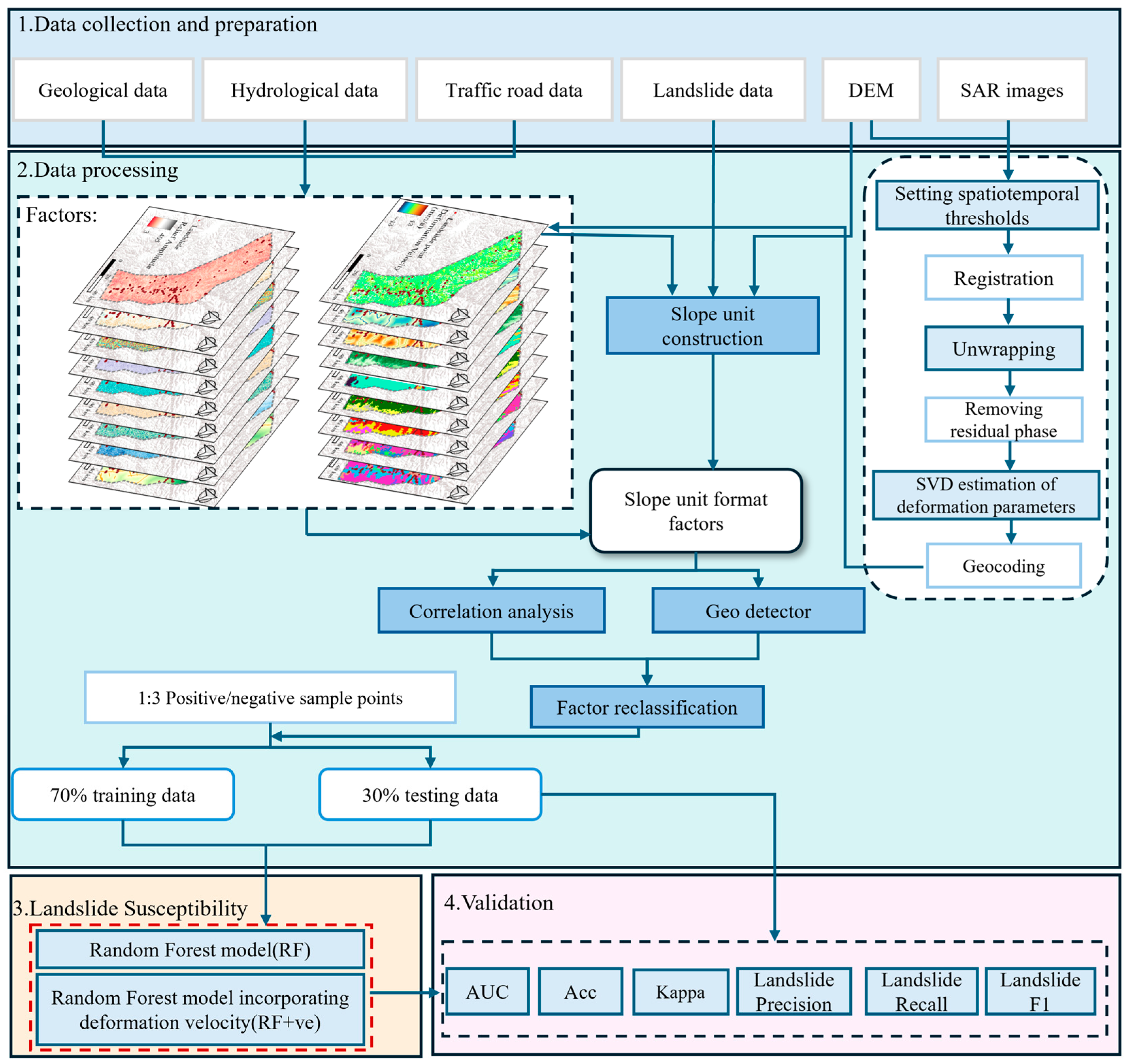
Figure 4 illustrates the methodological workflow of landslide susceptibility assessment, including data acquisition, factor preprocessing, slope unit partitioning, model construction, and accuracy validation.

3.1. Time-Series InSAR Surface Deformation Monitoring Method

The Small Baseline Subset Interferometric Synthetic Aperture Radar (SBAS-InSAR) technique enables high-resolution surface deformation monitoring through optimized interferometric pair selection. This approach significantly improves deformation retrieval accuracy while mitigating decorrelation effects and digital elevation model (DEM)-related phase errors—particularly valuable in steep, densely vegetated mountainous terrain.
The SBAS-InSAR processing was conducted using the SBAS module in SARscape software (v5.7.0, integrated within ENVI 5.6). The key steps and parameters are outlined as follows:
  • Spatiotemporal Baseline Thresholding: Define temporal and perpendicular baseline thresholds to select interferometric pairs with high coherence.
  • Image Co-Registration: Achieve pixel-level alignment for all selected pairs to ensure phase accuracy.
  • Phase Unwrapping: Retrieve absolute phase values from wrapped interferograms by resolving the 2π ambiguity. A coherence threshold of 0.1 was applied to select reliable pixels for unwrapping and subsequent time-series analysis.
  • Residual Phase Removal: Non-deformation components—including orbital errors, atmospheric delays, and DEM residuals—were mitigated. Precise Orbit Ephemerides from the European Space Agency (ESA) were incorporated to enhance orbital accuracy. For atmospheric correction, the method proposed by [57] was employed due to its efficacy in topographically complex regions, outperforming generic models in reducing topography-correlated atmospheric delays.
  • Reference Frame: The reference point was automatically established by the software based on the average elevation of the input SRTM 1-arc-second DEM across the entire scene, ensuring a stable and unbiased reference.
  • Deformation Time-Series Inversion: Establish linear equations across interferometric pairs and apply Singular Value Decomposition (SVD) to stably invert displacement values at each epoch.
  • Geocoding: The final deformation results in radar coordinates were transformed into geographic coordinates with a spatial resolution of approximately 15 m, ready for GIS integration.
A standard sign convention for line-of-sight (LOS) deformation was adopted: movement toward the satellite is considered positive (indicating uplift), and movement away from the satellite is negative (indicating subsidence).

3.2. Slope Unit Delineation

Slope units were delineated using the r.slopeunits module in GRASS GIS [58]. This algorithm utilizes digital elevation model (DEM) data and applies morphometric watershed segmentation combined with slope aspect homogeneity constraints to partition geomorphologically coherent natural slope boundaries. Compared to conventional raster-based units, this method reduces intra-unit terrain variance, enhances sensitivity to key landslide-controlling factors, and improves both the spatial reliability and interpretability of susceptibility mapping results.

3.3. Factor Selection

Candidate conditioning factors in landslide susceptibility modeling often exhibit information redundancy and multicollinearity, which can negatively affect model performance and interpretability. To mitigate these issues, this study conducted linear correlation analysis, multicollinearity diagnostics, and Geodetector to identify minimally correlated and representative input factors.

3.3.1. Pearson Linear Correlation Analysis

Principle: Pearson linear correlation analysis quantifies the strength and direction of the linear relationship between two variables:
r x y = i = 1 n x i x y i y i = 1 n x i x 2 i = 1 n y i y 2
r x y 1,1 ; the larger the absolute value, the stronger the correlation.
It is widely used in remote sensing and geomorphological studies to identify significant correlations between environmental variables and landslide occurrence. In general, an absolute correlation coefficient (|r|) below 0.5 is considered to indicate a weak relationship, and such variables are typically regarded as low collinearity.
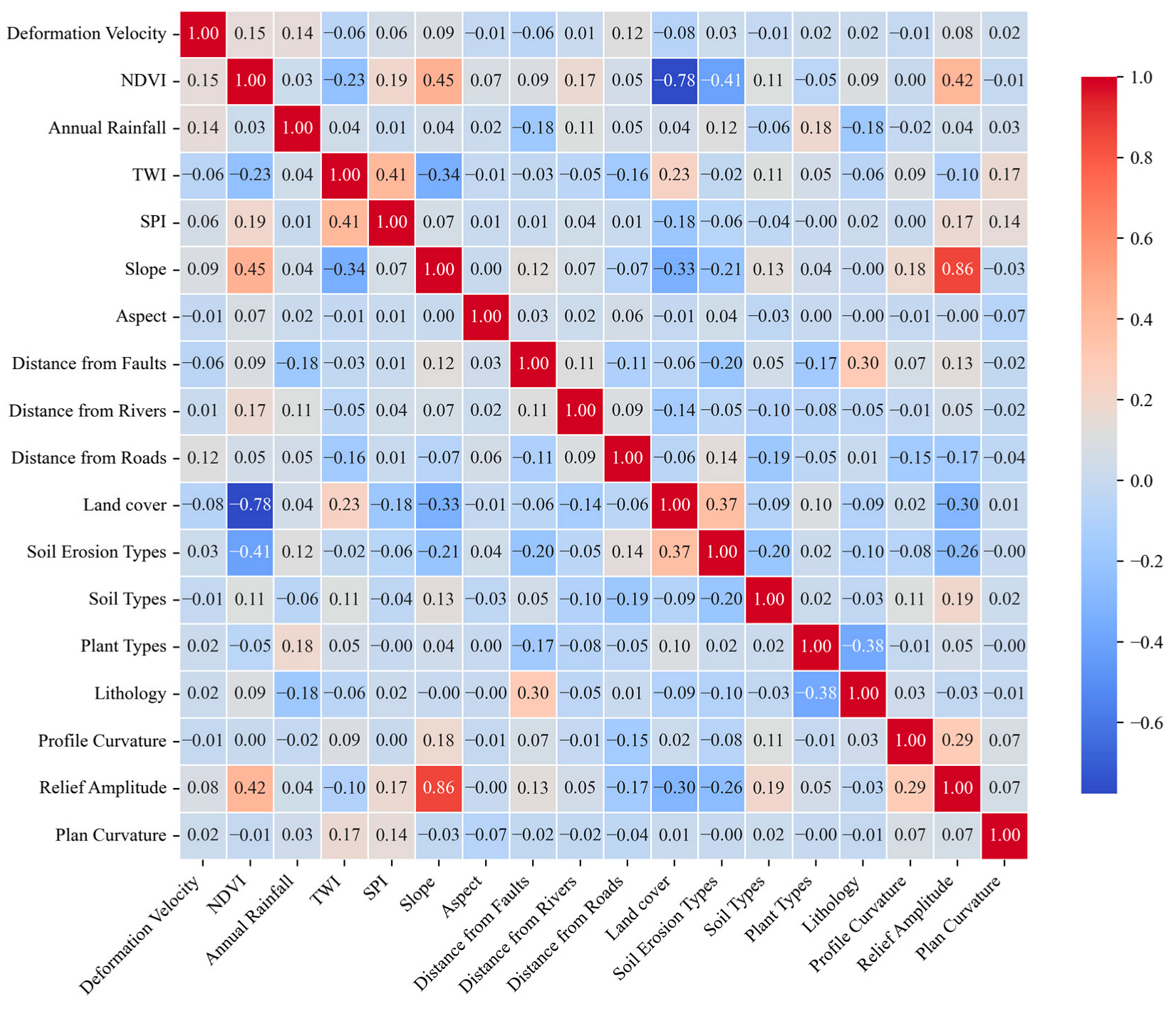
In this study, the Pearson correlation coefficients for the 18 conditioning factors (as described in Section 2.3) are summarized in Figure 5. The analysis revealed that land use and NDVI exhibited a strong negative correlation (r = −0.78), while topographic relief and slope showed a high positive correlation (r = 0.86). These two pairs indicate significant redundancy and may warrant the exclusion of one variable from each pair in subsequent modeling. All other factor pairs exhibited correlation coefficients with absolute values below 0.5.

3.3.2. Multicollinearity Testing-VIF/TOL

To further eliminate multicollinearity among the conditioning factors, this study employed the Variance Inflation Factor (VIF) and Tolerance (TOL) metrics to assess the severity of linear dependence among the selected factors.
The Variance Inflation Factor (VIF) quantifies how much the variance of a regression coefficient is inflated due to collinearity with other factors. It is calculated as
V I F j = 1 1 R j 2
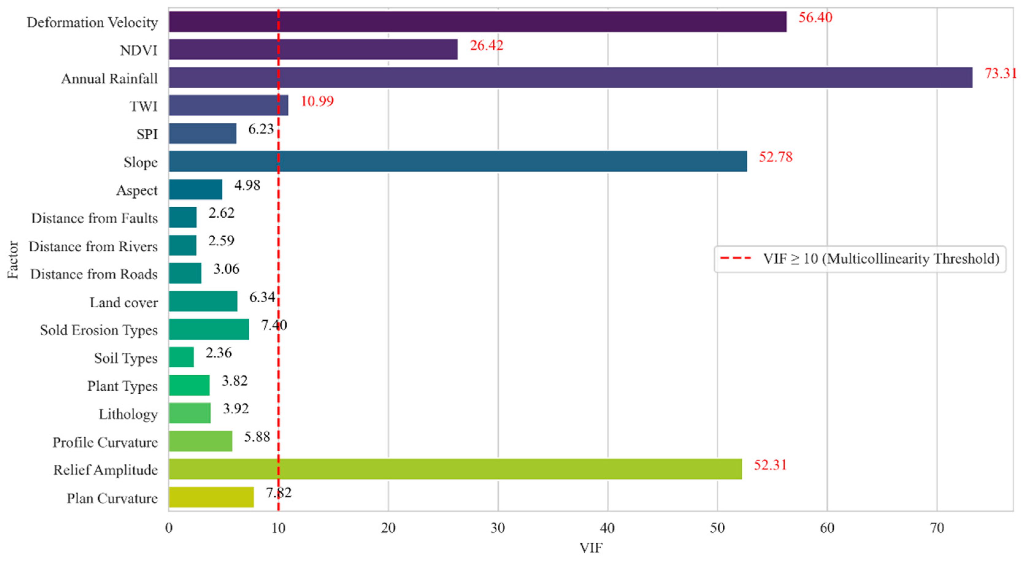
where R j 2 is the coefficient of determination when the j-th conditioning factor is regressed on all other factors. A VIF value greater than 10 is commonly considered indicative of serious multicollinearity.
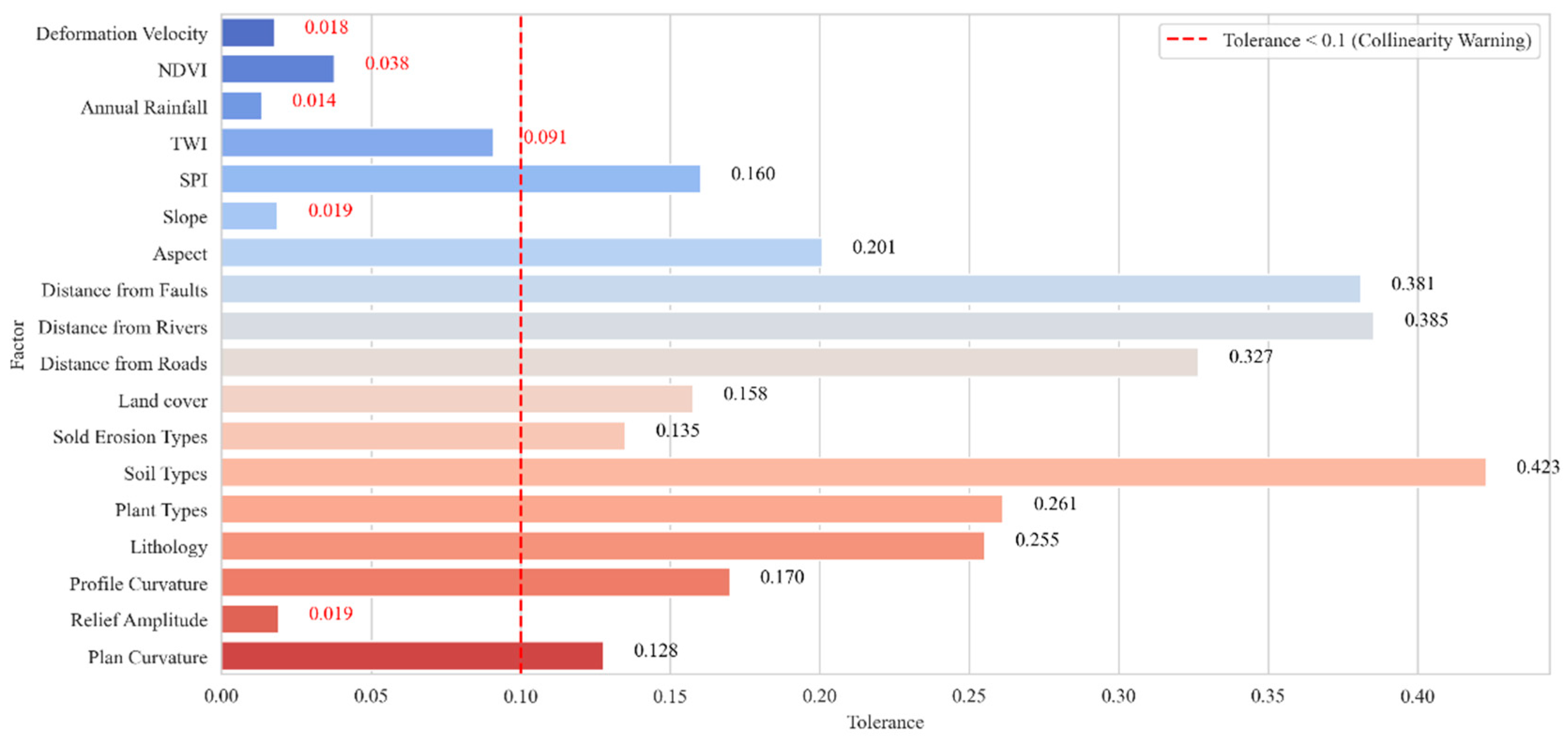
Correspondingly, the Tolerance (TOL), defined as
T O L j = 1 V I F j
Provides an inverse measure of collinearity, with TOL values below 0.1 generally indicating problematic collinearity. This step ensures that the final set of variables used in the susceptibility modeling process exhibits acceptably low linear dependence, thereby enhancing the robustness and interpretability of the model outputs. Six factors, including Annual Rainfall, Deformation Velocity, Slope, Relief Amplitude, NDVI, and TWI, did not meet the multicollinearity criteria based on VIF and TOL analyses (Figure 6 and Figure 7), and were subsequently subjected to further evaluation using the Geodetector-based factor detection method.

3.3.3. Dominant Factor Identification Via Factor Detector

To quantitatively assess the explanatory power of each factor on landslide susceptibility, this study employs the Factor Detector and Interaction Detector modules from the GeoDetector toolset [59]. The Factor Detector computes the explanatory power (q-value) of an independent variable X on a dependent variable Y, reflecting the extent to which the spatial variance in Y can be attributed to X. The formula is expressed as
q = 1 h = 1 L N h σ h 2 N σ 2
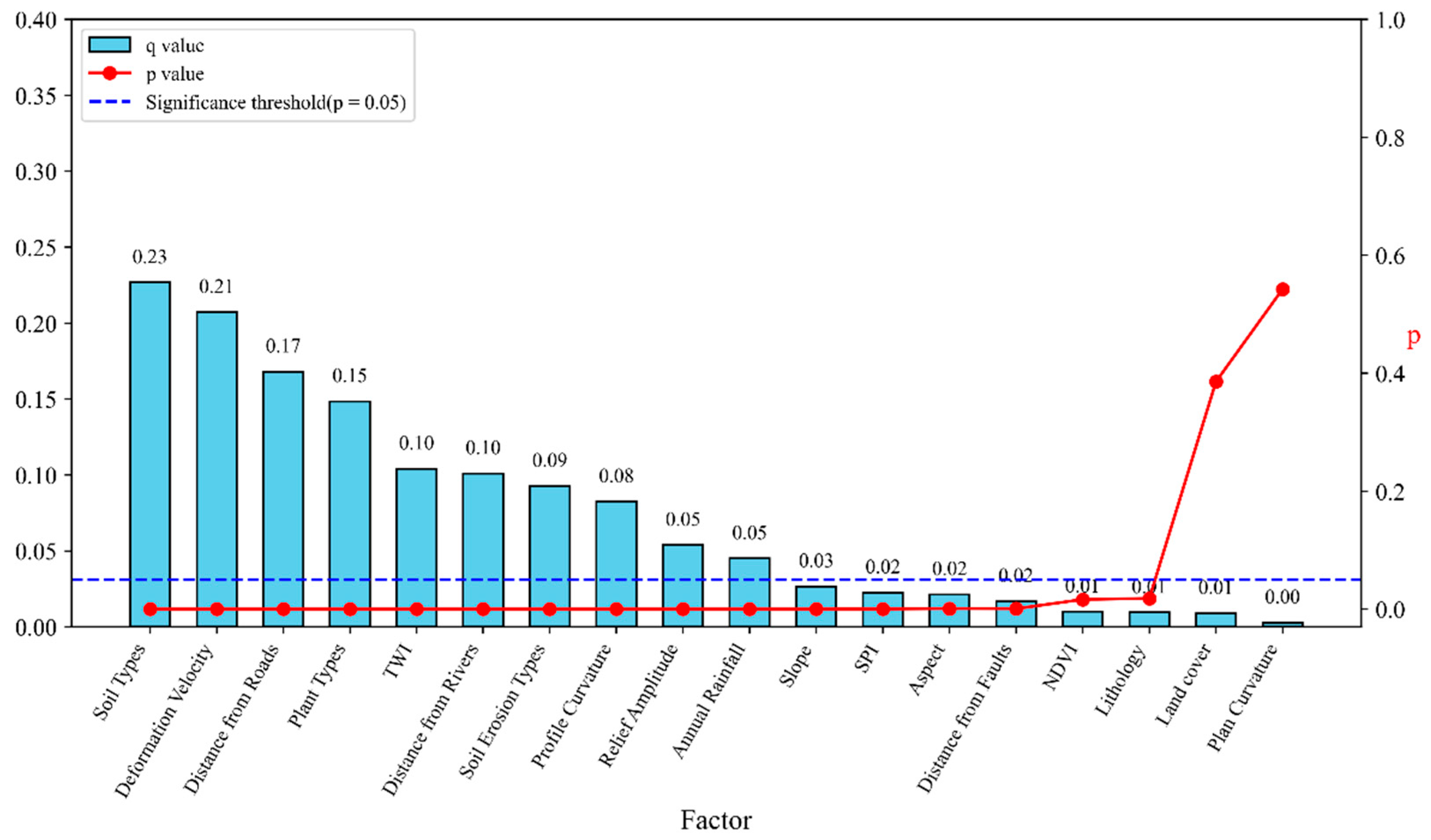
where L is the number of strata (or classes) of factor X, Nh is the number of samples in stratum h, σ_h2 is the within-stratum variance, N is the total number of samples, and σ2 is the overall variance of Y. The q-value ranges from 0 to 1, with higher values indicating greater explanatory power of the factor. Statistical significance was evaluated using the conventional p < 0.05 threshold, following standard statistical practice and established conventions in GeoDetector applications. A result with p < 0.05 is generally considered statistically reliable, indicating that the observed effect is unlikely to be due to random chance alone [60].
As shown in Figure 8, the top three factors with the highest q-values in this study are Soil Types, Deformation Velocity, and Distance from Roads, all of which also exhibit statistically significant p-values (p < 0.05). This suggests that these factors not only exhibit the strongest statistical association with landslide susceptibility but that these associations are highly unlikely to be due to chance. In contrast, the three lowest-ranking factors (Lithology, Land Cover, and Plan Curvature) demonstrate limited individual explanatory power; notably, Land cover and Plan Curvature also show non-significant p-values, further confirming their marginal role in the model.

3.4. Susceptibility Model Construction

To achieve accurate identification and refined classification of landslide susceptibility zones, this study employs the Random Forest (RF) model as the core probabilistic predictor. As an ensemble learning method, RF exhibits strong nonlinear modeling capability and robust resistance to overfitting, effectively handling high-dimensional geospatial covariates while demonstrating resilience to outliers and missing values. These advantages have led to the widespread application of RF in recent geological hazard susceptibility studies [61,62,63,64].
This study establishes two model configurations for comparative analysis: (A) the baseline RF model and (B) the optimized RF+ve model incorporating InSAR-derived deformation factors, aimed at systematically evaluating the enhancement in predictive performance attributable to deformation information. Building on prior findings that Bayesian optimization algorithms offer stable and efficient hyperparameter tuning for machine learning models [65,66], we introduce this approach to automatically adjust key RF hyperparameters, including the number of trees, maximum depth, and node splitting criteria. The optimization target is the mean AUC under 10-fold cross-validation, with iterative search yielding the optimal parameter set to construct a superior classification model.
Furthermore, the training sample set maintains a landslide-to-non-landslide label ratio of 1:3, reflecting both previous analyses of class imbalance in landslide inventories [67,68,69] and the uneven spatial distribution of landslides within the study area. Specifically, the dataset comprising 308 mapped landslides was randomly divided using a stratified sampling strategy: 70% of the samples (216 landslides and the corresponding non-landslide samples) were used to train the random forest model, while the remaining 30% (92 landslides and their corresponding non-landslide samples) were reserved as an independent testing set. The model training was performed solely on the training subset, and all accuracy metrics were evaluated exclusively on this independent testing dataset to avoid overfitting and ensure unbiased performance assessment. This sampling strategy mitigates model-improving performance in imbalanced classification scenarios.

3.5. Accuracy Assessment

To comprehensively evaluate the predictive performance of susceptibility probability models, multiple performance metrics were employed, including the Area Under the Receiver Operating Characteristic Curve (AUC), Kappa coefficient, Accuracy, Landslide Precision, Landslide Recall, and Landslide F1-score. These metrics collectively assess overall prediction accuracy, agreement between predicted and observed spatial patterns, model discriminative ability, and landslide detection effectiveness. The definitions of each metric are as follows:
(1) Area Under the ROC Curve (AUC)
The AUC reflects the model’s ability to rank landslide-prone and non-landslide areas. A higher AUC indicates better ranking capability. The ROC curve plots the true positive rate (TPR) against the false positive rate (FPR) and is defined as
T P R = T P T P + F N
F P R = F P F P + T N
(2) Kappa Coefficient
The Kappa coefficient quantifies the agreement between model predictions and actual classifications beyond random chance, and is calculated as
κ = P o P e 1 P e
where
P o = T P + T N N : Observed agreement (i.e., Accuracy)
P e = T P + F P T P + F N + F N + T N F P + T N N 2 : Expected agreement by chance
N: Total number of samples
Kappa value approaching 1 indicates high model reliability.
(3) Overall Accuracy (Accuracy)
Accuracy represents the proportion of correctly predicted samples among the total number of samples and is defined as
A c c u r a c y = T P + T N T P + T N + F P + F N
where
TP (True Positive): Landslide slope units correctly classified as landslide
TN (True Negative): Non-landslide pixels correctly classified as non-landslide
FP (False Positive): Non-landslide pixels incorrectly classified as landslide
FN (False Negative): Landslide pixels incorrectly classified as non-landslide
(4) Landslide Precision
Landslide precision measures the proportion of predicted landslide samples that are actually landslides:
P r e c i s i o n = T P T P + F P
(5) Landslide Recall
Landslide recall indicates the proportion of actual landslides that were correctly identified by the model:
R e c a l l = T P T P + F N
(6) Landslide F1
The F1-score is the harmonic mean of precision and recall, offering a balanced evaluation of both correctness and completeness in landslide classification:
F 1 = 2 × P r e c i s i o n × R e c a l l P r e c i s i o n + R e c a l l

4. Results

4.1. Surface Deformation Results from SBAS-InSAR

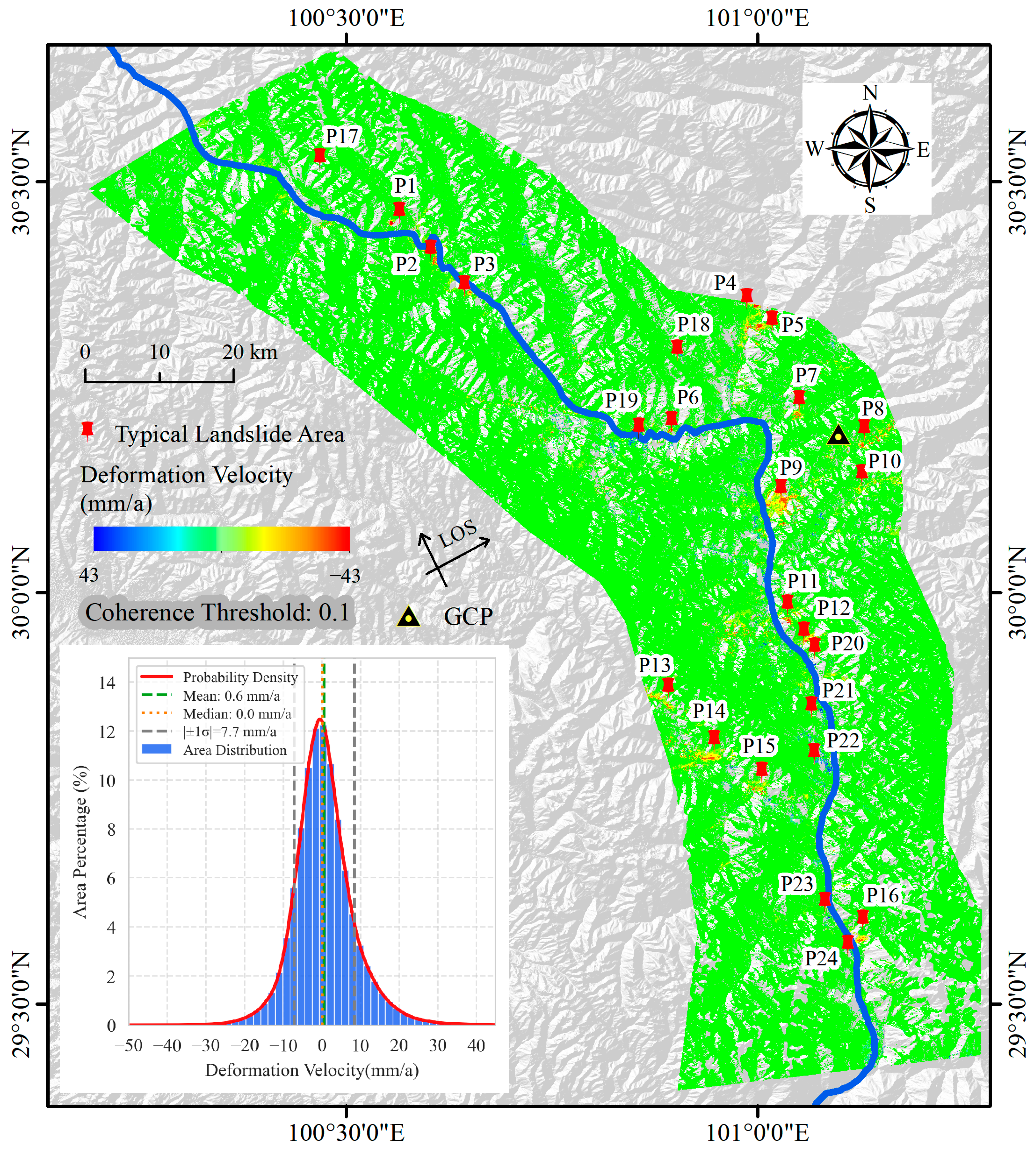
Figure 9 presents the spatial distribution map and histogram of Line-of-Sight (LOS) deformation velocity derived from May 2020 to May 2023. The deformation velocity follows an approximately normal distribution, centered at 0.6 mm/a with a standard deviation of 7.7 mm/a. The probability density function (red curve) and the mean ±1σ interval (−7.1 to +8.3 mm/a, shown as gray dashed lines) encompass approximately 68% of all pixels, further confirming that the majority of the region exhibits negligible deformation. More than 80% of the pixel values fall within the range of −10 to +10 mm/a (approximately ±1.3σ), indicating overall regional stability.
Building on previous studies [70], areas with velocity magnitudes exceeding 25 mm/a—defined as values beyond three standard deviations (3σ) from the mean—were identified as potential landslide zones. A total of 24 active deformation zones were delineated based on this threshold. Among these, 16 zones (P1–P16) exhibited positive LOS displacement, while 8 zones (P17–P24) showed negative LOS displacement.
Although these high-deformation areas account for less than 2% of the total study area, they represent concentrated geohazard zones and should be prioritized for further monitoring and risk mitigation.
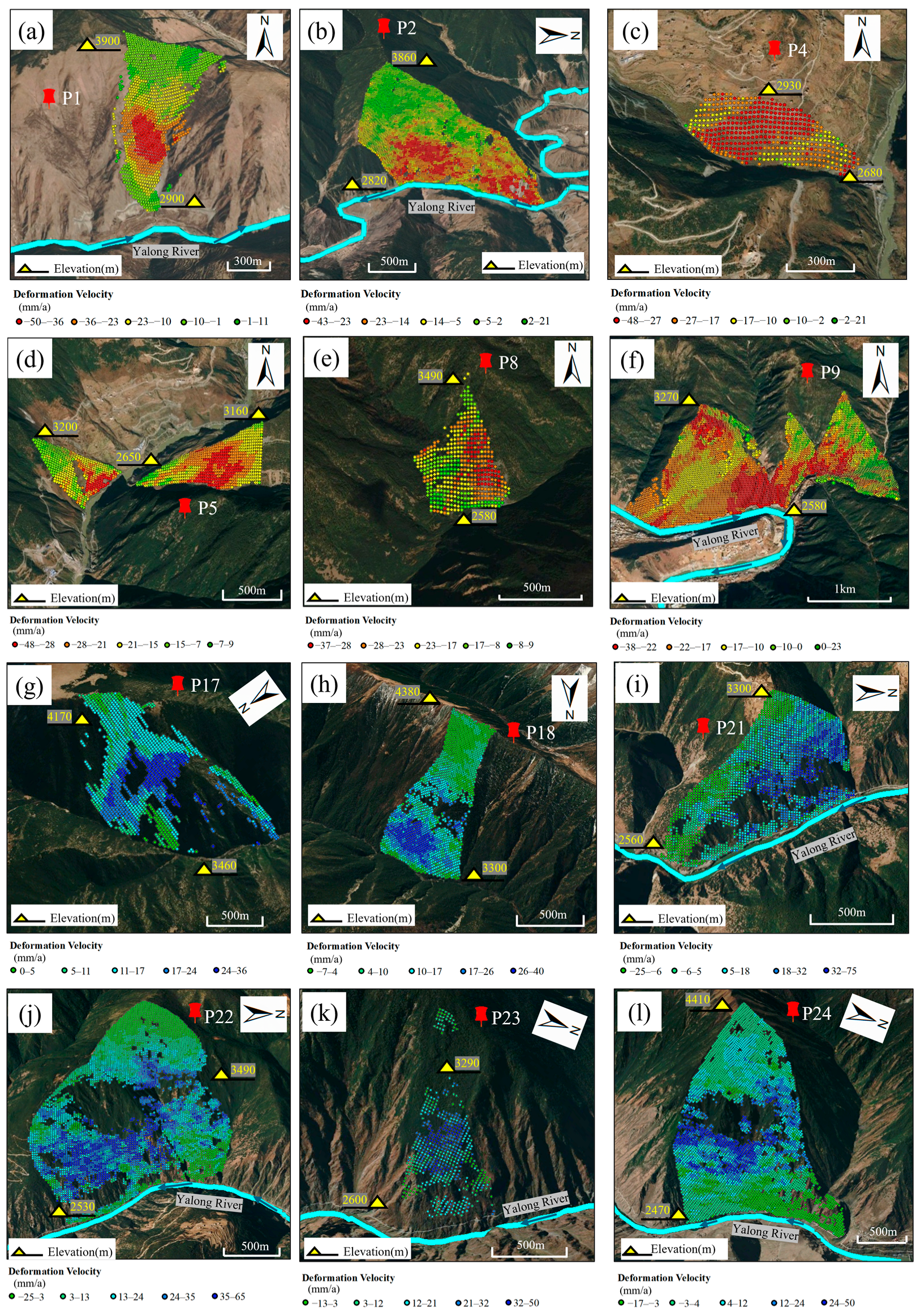
Figure 10 displays SBAS-InSAR-derived annual deformation velocity fields across representative landslide-prone areas. Figure 10a–f show deformation away from the satellite’s line-of-sight (LOS), while Figure 10g–l depict movement toward the LOS. Landslide activity clusters along the Yalong River mainstream, concentrating on steep valley slopes (>30°) with >500 m relief. These zones are governed by compound dynamics—fluvial incision, gravitational stress, and groundwater seepage—resulting in frequent deep-seated, slope-parallel sliding with deformation velocity exceeding 25 mm/a.
Actively deforming landslide zones are predominantly located in bare or sparsely vegetated areas, where high radar coherence allows for dense measurement points and reliable deformation signal retrieval. This enables accurate delineation of landslide boundaries and facilitates slope movement pattern analysis. Although dense vegetation may locally reduce coherence, the spatial distribution of unstable slopes remains clearly identifiable across the imagery, ensuring robust detection capability.
In summary, SBAS-InSAR enables high-resolution, large-scale deformation monitoring in landslide-prone terrains. The resulting deformation fields capture key geomorphic controls and spatial patterns of slope instability, and serve as critical inputs for slope unit delineation and data-driven susceptibility modeling.

4.2. Slope Unit Delineation Results

To ensure spatial compatibility between the evaluation units and actual landslide distributions, a minimum slope unit area threshold of 0.2 km2 (200,000 m2) was set using the GRASS GIS module r.slopeunits. This configuration helps resolve scale mismatches between unit boundaries and landslide boundary protrusions that may result from oversegmentation. Although the module itself does not incorporate deformation parameters, a circular variance threshold of 0.5 was applied—guided by SBAS-InSAR-identified geomorphic features such as main scarps and lateral boundaries—to improve alignment with observed landslide patterns. This approach maintains the structural characteristics of potential deformation zones while ensuring internal topographic homogeneity within slope units.
Iterative parameters included a reduction factor of 6, which controls the degree of slope unit subdivision in each iteration and reduces over-fragmentation in steep and heterogeneous terrains, and a maximum iteration limit of 2, which restricts the number of subdivision cycles to prevent excessive computational complexity and overly fragmented slope units. These settings were chosen to balance the preservation of terrain complexity with the scale of deformation features in the study area. The resulting slope units achieve compatibility with InSAR-derived deformation resolution while preserving intra-landslide heterogeneity.
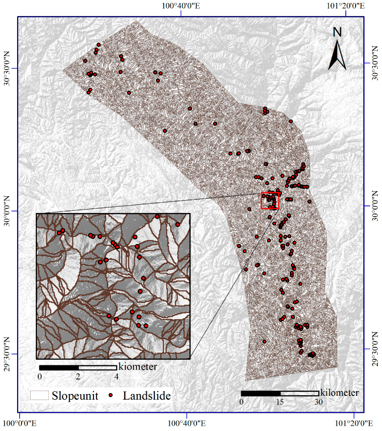
The delineation process generated 32,628 slope units. Each unit incorporates up to three historical landslide inventories, establishing a robust spatial foundation for susceptibility modeling. Figure 11 displays the spatial distribution of slope units across the study area.
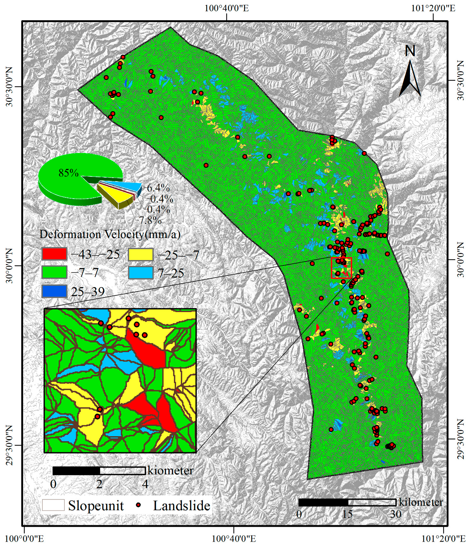
Figure 12 presents the spatial distribution of annual average surface deformation velocity across slope units. To mitigate atmospheric phase delays—prevalent in alpine canyons—and enhance modeling data reliability, the mean deformation velocity for each slope unit was extracted. Based on the natural breaks method and considering regional geomorphological characteristics, the deformation velocity was further categorized into five distinct classes:
  • −43 to −25 mm/a
  • −25 to −7 mm/a
  • −7 to 7 mm/a
  • 7 to 25 mm/a
  • 25 to 39 mm/a
Approximately 85% of slope units exhibit deformation velocity within ±7 mm/a, indicating regional surface stability. The second most prevalent category (−25 to −7 mm/a—7.8%, 7–25 mm/a—6.4%) concentrates in fragmented, steep terrain. High-magnitude deformation units are far less frequent (−43 to −25 mm/a—0.4%, 25–39 mm/a—0.4%).

4.3. Model Comparison Results

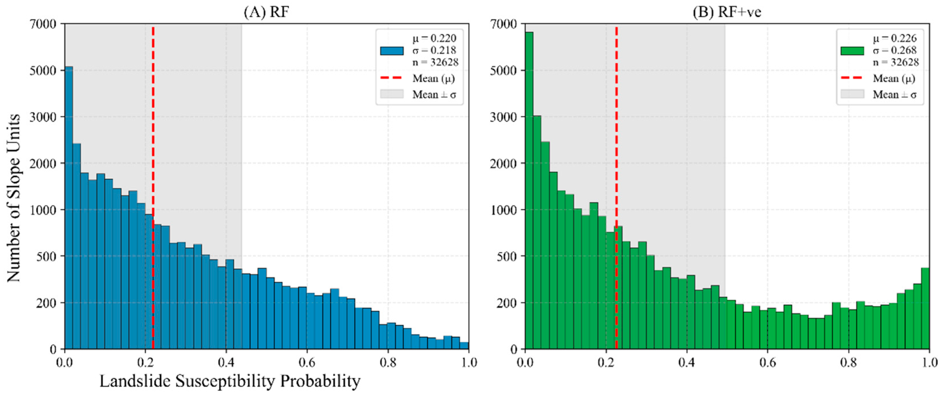
To investigate the role of deformation velocity in landslide susceptibility assessment, this study designed a comparative experiment based on the Random Forest (RF) model. Two model configurations were constructed: Model A (RF), serving as the baseline without incorporating deformation factors, and Model B (RF+ve), an enhanced version integrating deformation velocity. Figure 13 illustrates the probability distribution of landslide susceptibility predicted by both models across slope units, with annotations for the mean (μ), standard deviation (σ), and sample size (n). The red dashed line represents the mean prediction, while the gray shaded area denotes the interval of one standard deviation above and below the mean.
Overall, both models exhibit a pronounced right-skewed distribution, with the majority of slope units falling within the low-probability range (<0.4), and relatively fewer units predicted with high susceptibility (>0.6), reflecting the models’ strong effective risk stratification. In comparison, although both models yield similarly low mean values (0.220 for RF and 0.226 for RF+ve) and comparable standard deviations, indicating robust classification performance, the inclusion of surface deformation leads to a notable increase in the number of slope units assigned high susceptibility probabilities (>0.6). This results in a heavier distribution tail, suggesting that the incorporation of deformation information enhances the model’s sensitivity to areas characterized by strong surface activity and elevated landslide potential. Consequently, such integration aids in identifying critical high-risk zones that might otherwise be underestimated in baseline assessments.
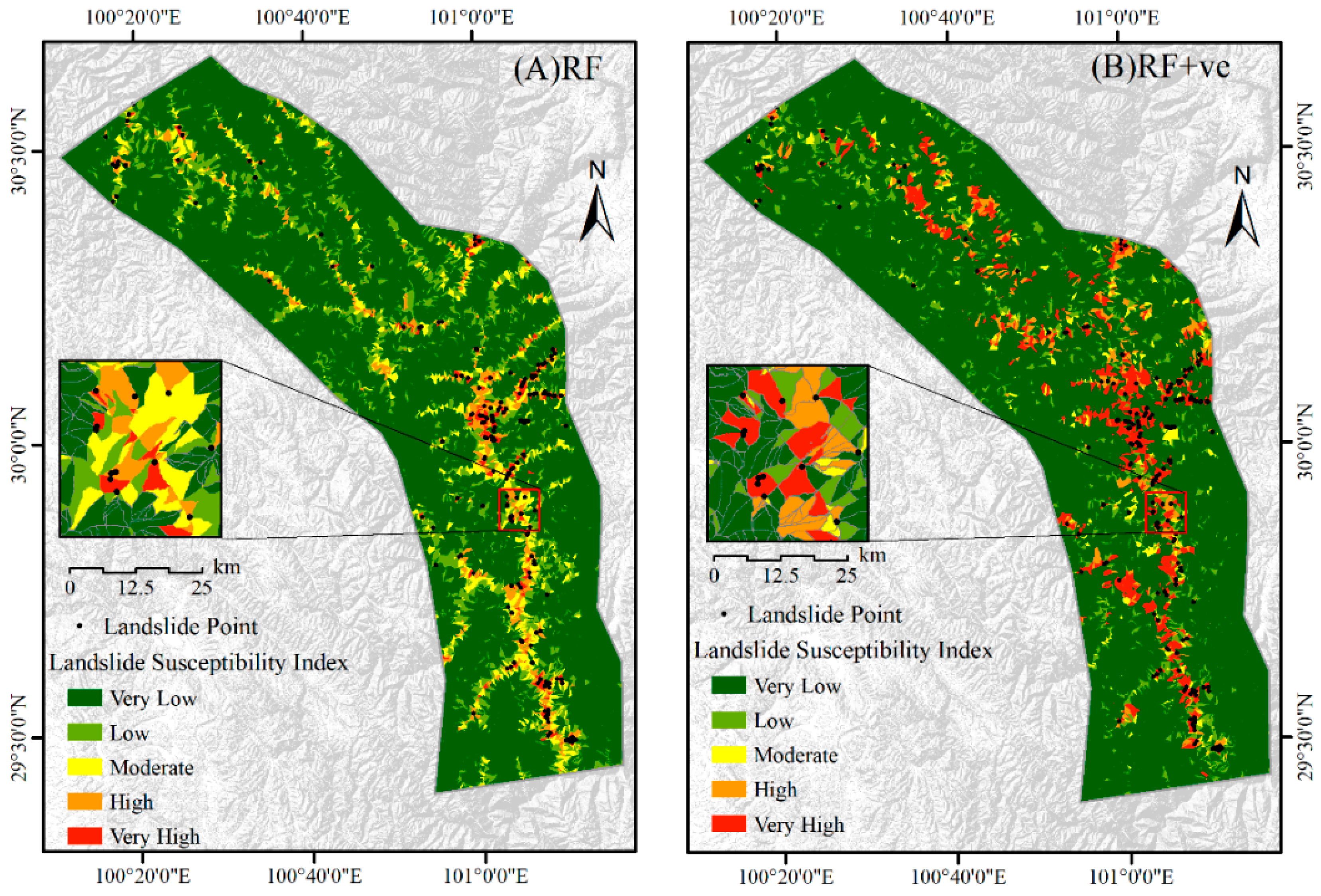
To visually characterize the spatial distribution patterns of model predictions, the landslide susceptibility probabilities were classified into five categories using an equal-interval method: Very Low (0–0.2), Low (0.2–0.4), Moderate (0.4–0.6), High (0.6–0.8), and Very High (0.8–1.0). Figure 14 presents the spatial prediction maps generated by the baseline RF model (A) and the enhanced RF+ve model (B), respectively. To assess the predictive validity of each model, historical landslide occurrences were overlaid on the susceptibility maps.
From a spatial perspective, the incorporation of surface deformation significantly enhances the model’s ability to delineate high-susceptibility zones with greater continuity and concentration, particularly in areas with dense landslide occurrences. In the eastern slope regions, areas classified as “Very High” susceptibility by the RF+ve model exhibit a high degree of spatial agreement with known landslide locations, demonstrating improved localization and boundary definition of high-risk zones. Notably, the RF+ve model also identifies a “Very High” susceptibility zone in the northwestern sector (30°30′N, 100°40′E), where no historical landslides have been recorded so far, suggesting potential for early-stage surface deformation monitoring and proactive landslide risk management in this area. In contrast, the baseline RF model, which lacks deformation input, tends to underestimate susceptibility in certain regions—misclassifying some confirmed landslide points into moderate or low susceptibility classes. This discrepancy reveals the baseline model’s limited capacity to capture spatial heterogeneity in landslide-prone terrains.
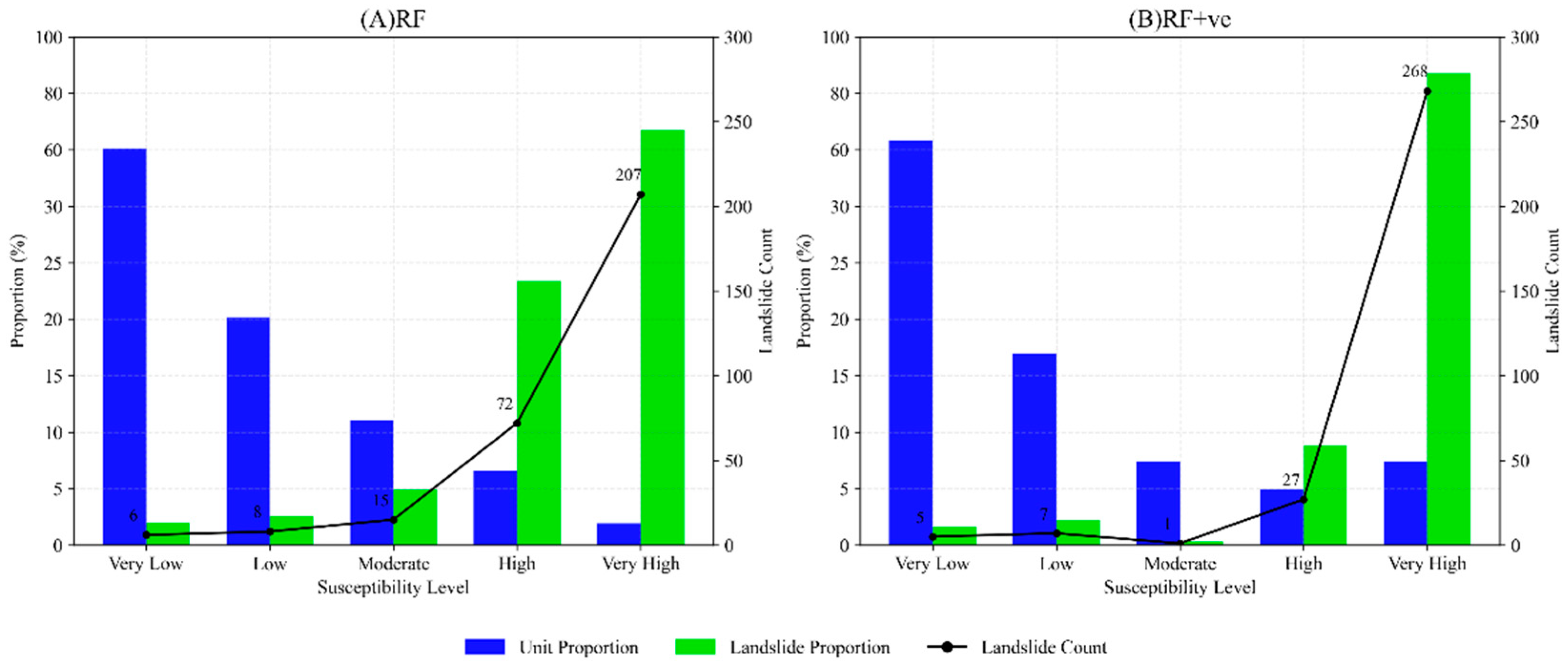
To further evaluate the performance of susceptibility classification, Figure 15 summarizes the proportion of slope units, the proportion of historical landslide occurrences, and the absolute number of landslide points across different susceptibility levels.
The results indicate that, within the “Very High” susceptibility class, the number of landslide occurrences identified by the RF+ve model increased from 207 to 268, with the capture rate increasing from 67.21% to 87.01%. Simultaneously, the proportion of slope units in this class rose from 2% to 7%, and the percentage of landslide points increased from 67% to 87%, highlighting a substantial enhancement in the model’s capability to identify high-risk areas. In addition, the number of landslide points within the Moderate and High classes decreased significantly—from 15 to 1 and from 72 to 27, respectively—indicating a marked shift toward the highest susceptibility class. This pattern suggests that the optimized model effectively reclassifies previously misclassified high-risk clusters, thereby improving the clarity and concentration of landslide hazard expression in the upper categories. In contrast, for the lower susceptibility levels (Very Low and Low), both models yield similar proportions of slope units (approximately 60% and 20%, respectively), and the number of associated landslide points remains in the single digits. This consistency demonstrates that model optimization does not compromise the reliable identification of low-risk areas, nor does it lead to an increase in false positives.
In summary, the integration of surface deformation factors enhances the model’s spatial heterogeneity characterization and susceptibility stratification capability. This improvement enables the model to more effectively concentrate on potential high-risk areas, thereby increasing the overall accuracy and practical applicability of the landslide risk assessment.
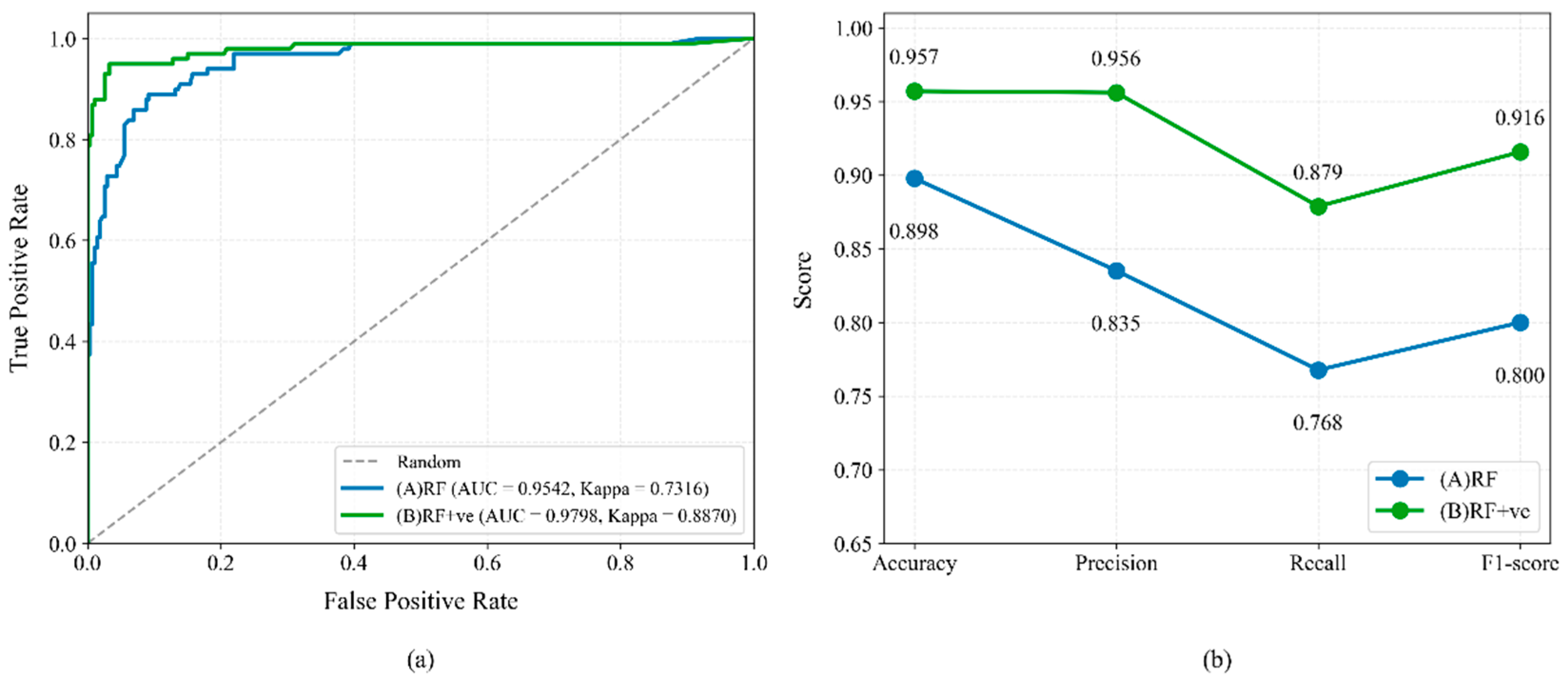
To quantitatively evaluate the overall classification performance of the models, Figure 16a presents a comparison of the Receiver Operating Characteristic (ROC) curves for the RF and RF+ve models. The results indicate that the ROC curve of the RF+ve model is closer to the top-left corner, with the Area Under the Curve (AUC) improving from 0.9542 to 0.9798. Additionally, the Kappa coefficient rose markedly from 0.7316 to 0.8870. Both models significantly outperform the random guess baseline, confirming their reliable discriminative capabilities. However, the RF+ve model demonstrates superior overall performance in terms of both classification ability and accuracy.
Figure 16b further quantifies model performance across four commonly used evaluation metrics: Accuracy, Precision, Recall, and F1-score. Compared with the baseline RF model, the RF+ve model achieves consistent improvements across all metrics, including a 6.6% increase in Accuracy, 14.5% in Precision, 24.2% in Recall, and 19.1% in F1-score. These results suggest that the enhanced model not only maintains high predictive accuracy but also achieves a better balance between the identification of positive and negative samples. The overall improvement underscores the effectiveness of incorporating surface deformation factors in systematically enhancing model performance.
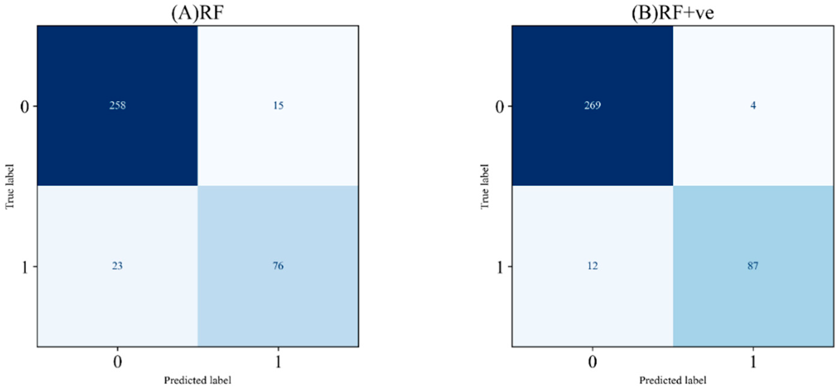
Figure 17 presents the confusion matrices of the two models, providing an intuitive comparison of their classification performance based on the independent testing dataset (92 landslide samples), and further validating the robustness and reliability of the RF+ve model in practical applications. In terms of error control, the number of false positives decreased substantially from 15 to 4 (a 73.3% reduction), while false negatives declined from 23 to 12 (a 47.8% reduction), indicating a significant reduction in both false alarms and missed detections of landslide events. Regarding the identification of positive and negative cases, the RF+ve model achieved an increase in true positives from 76 to 87 (a 14.5% improvement), while the number of true negatives remained at a high level (269), outperforming the RF model’s 258. These findings demonstrate that the RF+ve model not only improves overall classification accuracy but also enhances its ability to effectively focus on actual landslide-prone areas, thereby contributing to more reliable hazard identification in complex terrain settings.
In summary, the incorporation of InSAR-derived surface deformation velocity significantly enhances the overall performance and practical value of landslide susceptibility assessment models. Across multiple dimensions—including probability distribution characteristics, spatial clustering patterns, susceptibility classification, and classification accuracy metrics—the RF+ve model consistently outperforms the baseline RF model. Notably, in terms of high-risk area identification, the RF+ve model demonstrates a stronger capacity to concentrate landslide occurrences within the highest susceptibility classes while effectively reducing misclassifications and risk misclassification in intermediate classes in the intermediate categories. This reflects an improved ability to distinguish between varying levels of landslide risk and adapt to complex spatial heterogeneity.
Moreover, quantitative evaluation results—such as the ROC curves, classification metrics, and confusion matrices—further validate the systematic improvement brought by the deformation factor in terms of model stability, robustness, and discriminative power. These findings clearly demonstrate that integrating InSAR-based deformation information effectively addresses the limitations of conventional models in dynamic landslide detection and provides a feasible and methodologically robust framework for refined landslide risk assessment in mountainous canyon regions.

5. Discussion

5.1. Analysis of Factor Contributions

The spatiotemporal pattern of landslide susceptibility is fundamentally driven by the synergistic interaction of multiple factors. To systematically elucidate the individual contributions of each factor to model predictions as well as their interactive effects, this study integrates SHAP (Shapley Additive exPlanations) [71] and Geodetector techniques to conduct an in-depth analysis from both individual influence and interaction enhancement perspectives.
Regarding the SHAP analysis, positive SHAP values indicate that the presence or magnitude of a given factor increases the predicted probability of a landslide, thereby exerting a landslide-promoting effect. Conversely, negative SHAP values suggest that the factor reduces landslide probability, implying a protective or inhibiting effect.
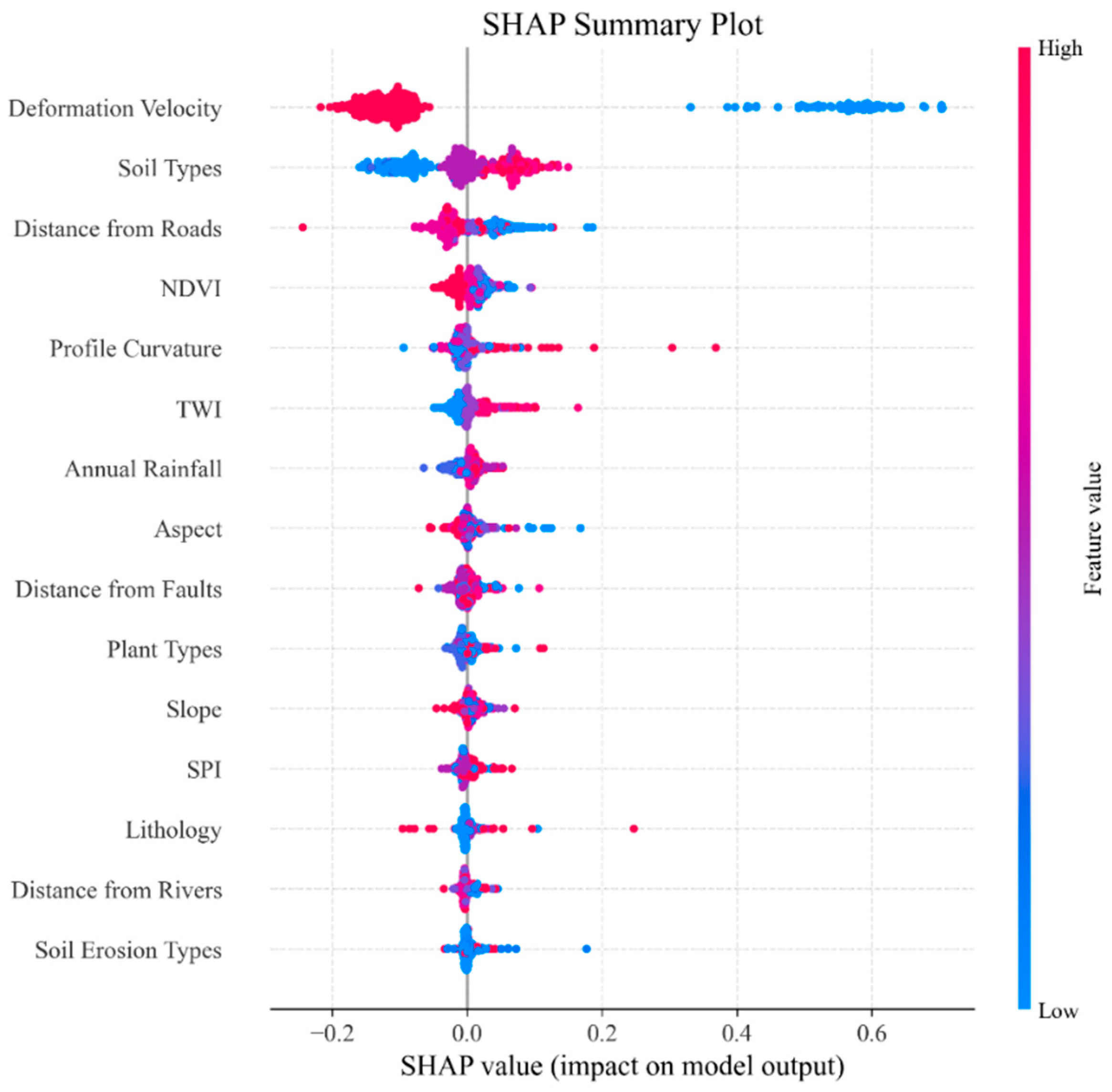
The global feature importance quantified by SHAP values (Figure 18) reveals the relative contributions and directional effects of the factors. The results indicate that the InSAR-derived annual deformation velocity exhibits the strongest predictive influence, characterized by the widest range of SHAP values predominantly reflecting the landslide-promoting effect. This finding directly confirms that surface deformation is a critical indicator of landslide initiation and activity, exerting a decisive impact on the model’s predictive outcomes. Other influential factors with notable effects on model outputs include soil types, distance from roads, profile curvature, and the topographic wetness index (TWI).
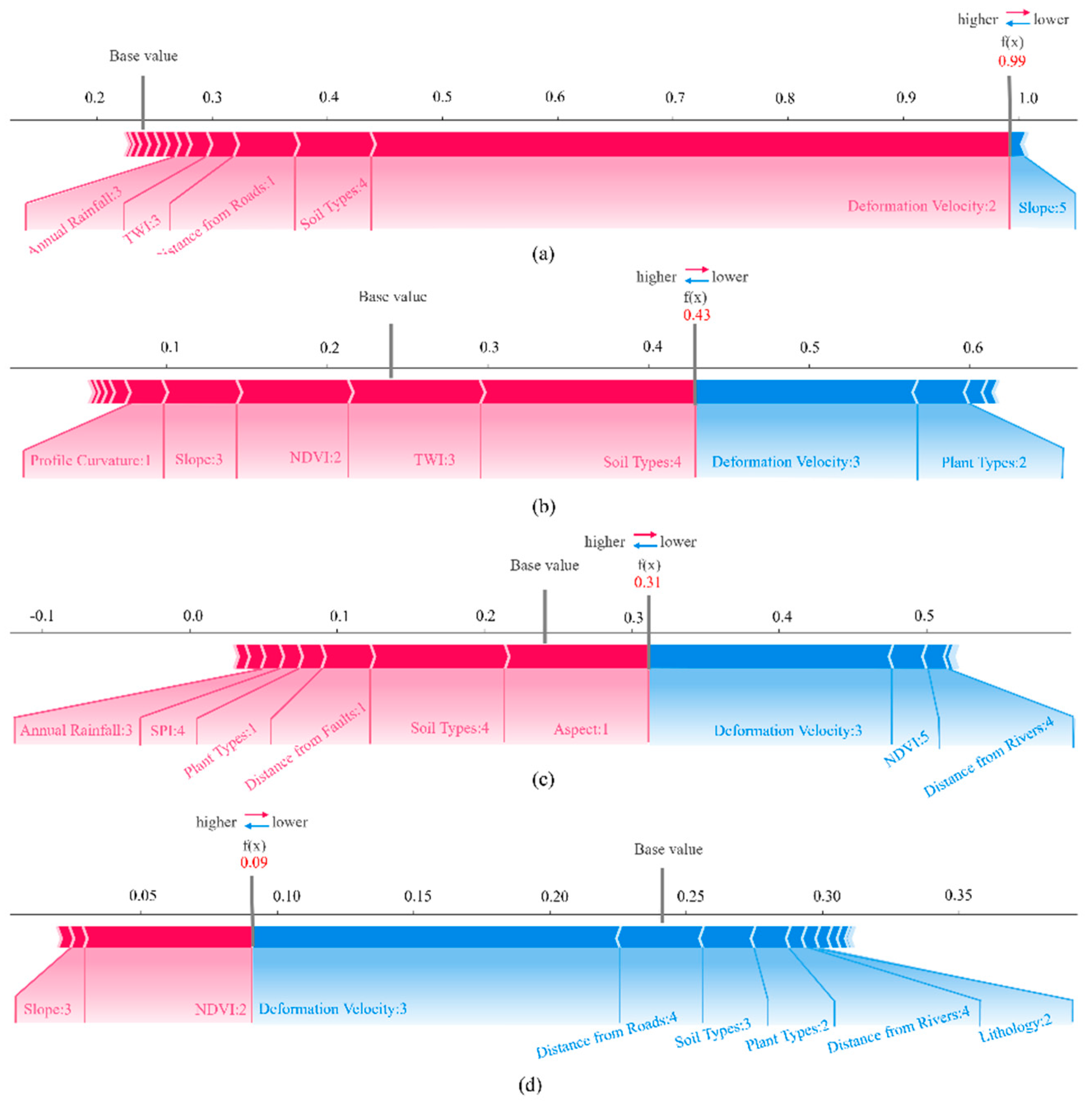
Figure 19 presents the SHAP force plot for an individual sample, which deconstructs the model’s prediction into the contributions of each feature. The plot shows how the progressive accumulation of multiple factors drives the landslide risk level for this specific case. The plot interprets the model’s output by comparing it to a base value—the average model prediction over the training dataset. The high-risk sample (a) exhibits several positively contributing risk features: an annual average LOS deformation velocity of 7–25 mm/a, indicating that the slope is undergoing intense and sustained deformation, which serves as a direct precursor to landslide occurrence; soil characterized as loose, unstable with low shear strength, making it highly susceptible to failure under saturated or disturbed conditions; proximity to roads within 1 km, suggesting significant influence from anthropogenic engineering activities such as cut slopes and embankments; and an annual rainfall ranging between 2600 and 2700 mm combined with a Topographic Wetness Index (TWI) of 6–8, highlighting strong regional moisture accumulation that can increase pore water pressure and further undermine slope stability. These factors collectively exert substantial positive SHAP values, driving the model output probability to 0.99, thus representing a typical synergistic failure mechanism pattern associated with high landslide risk.
In contrast, the low-to moderate-risk samples (e.g., (b) and (c)) generally exhibit stronger stability characteristics. Sample (b) (with a predicted probability of 0.43) shows an annual deformation rate below 7 mm/a and is characterized by vegetation types that contribute to soil reinforcement, reflected by mildly negative SHAP values indicating overall controlled risk. Sample (c) (probability 0.31) features minimal deformation, relatively high NDVI, and considerable distance from rivers. Although lithology and soil factors have limited influence, the combined effects of favorable ecological and hydrological conditions act to suppress landslide risk, maintaining it at a low level. The very low-risk sample (d) (probability 0.09) displays multiple stable factors acting synergistically: negligible deformation, remote location from roads and water bodies, moderately firm soil, and stable vegetation and lithology types.
Collectively, these analyses demonstrate that high-risk samples are driven by the synergistic amplification of multiple positively contributing conditioning factors, resulting in strong and concentrated hazard pressures. Conversely, low- to moderate-risk samples benefit from the combined effect of multiple negatively contributing factors, forming a dispersed yet resilient protective system. This contrast exemplifies a pattern of concentrated multi-hazard synergy versus distributed defense factors, highlighting the fundamental difference between zones dominated by compounding risk drivers and those characterized by systemic resistance to slope failure.
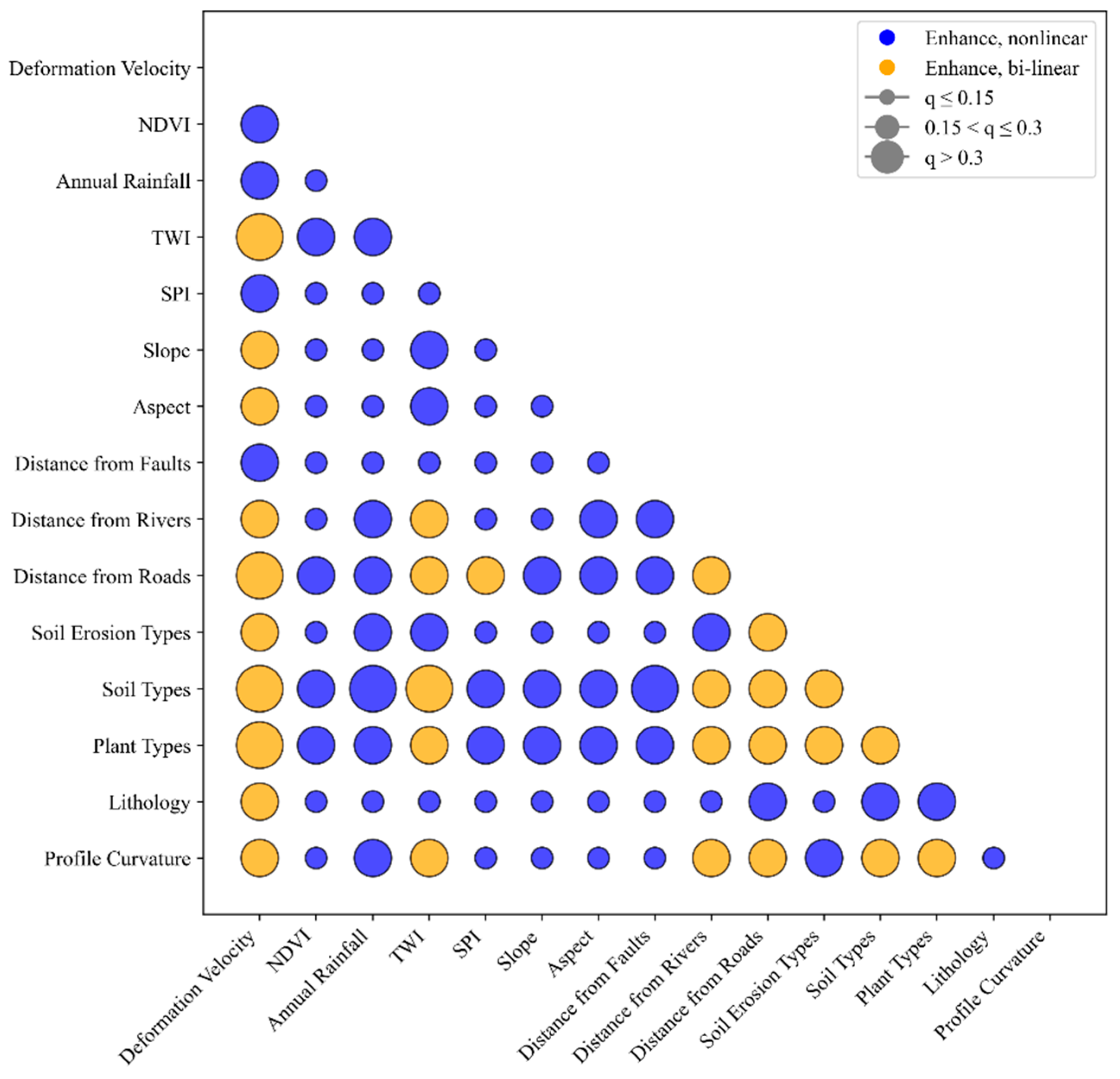
The interaction bubble plot of geodetector results shown in Figure 20 quantitatively reveals the coupling strength (q-values) among landslide-triggering factors, building upon the nonlinear synergistic interaction mechanism illustrated in Figure 19 and further elucidating the intrinsic logic of compound triggering processes. The results demonstrate that nonlinear synergistic enhancement effects are widespread across the study area, with the interaction between soil type and mean annual rainfall being the most prominent (q = 0.38), representing a primary controlling factor pair for landslide initiation. This mechanism explains the failure pathway of the high-risk sample (Figure 19a): loose soils rapidly saturate and lose strength under intense rainfall, ultimately triggering shallow landslides, which corresponds closely to the critical “soil–rainfall” coupling effect and aligns with the sample’s characteristic features of “intense deformation + high rainfall + loose soil.”
Distinct mechanistic differentiation is observed across risk levels: high-risk samples are predominantly governed by nonlinear coupling between soil and rainfall (q > 0.3), often compounded by engineering disturbances that form a anthropogenically triggered hydro-mechanical degradation cascade. In contrast, low- to moderate-risk samples are mainly influenced by linear enhancement between vegetation and topographic factors, where ecological slope stabilization and hydrological regulation mechanisms effectively mitigate risk. Overall, the significant variation in interaction strengths (q-values ranging from 0.15 to 0.38) indicates that static single-factor models are inadequate for accurately identifying compound triggering risks. Therefore, constructing dynamic coupled models that emphasize abrupt transitions within critical interaction chains such as “soil–rainfall” and “vegetation–topography” is essential to improving the accuracy and adaptability of landslide susceptibility assessments.

5.2. Applicability Analysis

The proposed landslide dynamic susceptibility assessment framework, which integrates time-series InSAR deformation monitoring with multi-factor interaction analysis, demonstrates significant scientific value and engineering applicability in the Yalong River basin case study.
Firstly, addressing the strong landslide activity and the time-varying trigger dynamics characteristic of canyon regions, the SBAS-InSAR technique provides annual deformation velocity fields that effectively capture the spatiotemporal heterogeneity of surface deformation. By jointly modeling this dynamic deformation information with static geological and environmental conditioning factors, the framework overcomes limitations of conventional static susceptibility assessments, which often fail to characterize the temporal complexity and initiation mechanisms of landslides. This approach is particularly suitable for areas subject to tectonic activity, seasonal precipitation variations, and anthropogenic slope modifications, such as road construction, excavation, or slope loading.
Secondly, by incorporating historical landslide data and InSAR-derived deformation zones, the slope unit delineation method was optimized to construct a more refined sample dataset. This approach significantly improves the internal homogeneity and boundary accuracy of geomorphic units, effectively mitigating the mismatch between spatial partitioning units and landslide formation mechanisms in complex terrain. The study provides a scalable and transferable technical framework for landslide susceptibility zoning in mountainous regions, including fold-thrust belts and incised alpine gorge landscapes.
Furthermore, the Geodetector-based quantification of interaction effects between factors such as “annual rainfall–soil type” reveals the coupled hydrogeological mechanisms governing landslide development in high mountain canyon areas, offering an effective tool for regional multi-layered disaster triggering mechanism studies.
Empirical results indicate that the AUC of the Random Forest model increased to 0.9798 after incorporating InSAR-derived deformation factors, demonstrating the effectiveness of integrating multi-source dynamic data with machine learning in improving landslide susceptibility discrimination capability. This framework provides strong practical value for landslide risk management in hydropower-concentrated areas of the eastern Tibetan Plateau and offers scientific support for major engineering site selection, disaster chain risk early warning, and territorial spatial planning.
It should be noted that the approach may be affected by reduced InSAR coherence in densely vegetated areas, requiring complementary optical remote sensing or multi-temporal interferometric optimization. The slope unit delineation algorithm’s parameter adaptation in extremely complex terrain requires further refinement to examine whether steep elevation gradients could cause over-segmentation or boundary misalignment of slope units. Additionally, the temporal response mechanisms of short-term disturbance factors such as extreme rainfall events relative to InSAR deformation data warrant deeper investigation. Overall, the proposed dynamic landslide susceptibility evaluation framework demonstrates strong potential for broader application, especially for risk management and mitigation in tectonically active and highly variable terrain regions.

6. Conclusions

(1)
A geodetector–random forest evaluation framework integrated with time-series InSAR monitoring was developed and applied to the Xinlong–Kangding section of the Yalong River Basin. Based on Sentinel-1 imagery acquired from 2020 to 2023, surface deformation velocities were derived using the SBAS-InSAR technique. The results identified 24 highly active landslide areas exhibiting annual average deformation velocity exceeding 25 mm/a.
(2)
By integrating InSAR-derived deformation data with historical landslide distributions, the delineation of slope units was optimized to construct a high-quality sample set for comparative experiments. The results demonstrate that the inclusion of deformation factors significantly enhances the model’s discriminative performance, with the AUC value increasing to 0.9798 and the Kappa coefficient rising to 0.8870. Additionally, the landslide containment rate in the Very High susceptibility class improved from 67.21% to 87.01%, a gain which we attribute to the way deformation velocity identifies and differentiates slopes exhibiting recent movement activity from those that are stable (particularly among areas with similar geological-geomorphological characteristics) and synergizes with static factors to better characterize spatial clustering patterns, particularly in response to recent triggering events. These findings confirm the efficacy of multi-source data integration in improving landslide susceptibility assessments in alpine canyon environments, and underscore its advantage in capturing spatially clustered landslide hazards.
(3)
Geodetector-based interaction analysis reveals that the nonlinear coupling between annual precipitation and soil type (q = 0.38) predominantly controls shallow landslide initiation, exhibiting a 15% improvement in explanatory power compared to individual factors. In contrast, terrain-related variables such as the Topographic Wetness Index (TWI) and distance to roads influence slope stability Via coupled effects from anthropogenic slope modifications and hydrological concentration, exhibiting a quasi-linear enhancement effect (q = 0.21). These spatial interaction patterns are corroborated by SHAP analysis, which highlights a distinctive contrast between spatially clustered hazards and distributed stabilizing factors, providing robust quantitative evidence for the compound, multi-source nature of landslide susceptibility differentiation.

Author Contributions

All the authors participated in editing and reviewing the manuscript. Writing—original draft, Z.L., conceptualization, J.X. and G.Z.; methodology, H.Z.; software, Z.L.; formal analysis, K.D. and X.S. All authors have read and agreed to the published version of the manuscript.

Funding

This work was supported in part by the National Natural Science Foundation of China under Grant 42371462, in part by Sichuan Province Science Fund for Distinguished Young Scholars under Grant 2023NSFSC1909, in part by the National Key Research and Development Program of China under Grant 2021YFB3901403, in part by Natural Science Foundation of Sichuan under Grant 22NSFSC0104, in part by Sichuan Society of Surveying Mapping and Geoinformation under Grant CCX202403.

Conflicts of Interest

The authors declare no conflicts of interest.

References

  1. Kirschbaum, D.B.; Adler, R.; Hong, Y.; Hill, S.; Lerner-Lam, A. A Global Landslide Catalog for Hazard Applications: Method, Results, and Limitations. Nat. Hazards 2010, 52, 561–575. [Google Scholar] [CrossRef]
  2. Petley, D. Global Patterns of Loss of Life from Landslides. Geology 2012, 40, 927–930. [Google Scholar] [CrossRef]
  3. Li, Y.; Chen, J.; Zhou, F.; Song, S.; Zhang, Y.; Gu, F.; Cao, C. Identification of Ancient River-Blocking Events and Analysis of the Mechanisms for the Formation of Landslide Dams in the Suwalong Section of the Upper Jinsha River, SE Tibetan Plateau. Geomorphology 2020, 368, 107351. [Google Scholar] [CrossRef]
  4. Pan, G.; Wang, L.; Li, R.; Yuan, S.; Ji, W.; Yin, F.; Zhang, W.; Wang, B. Tectonic Evolution of the Qinghai-Tibet Plateau. J. Asian Earth Sci. 2012, 53, 3–14. [Google Scholar] [CrossRef]
  5. Zhang, J.; Yang, R.; Qi, Y.; Zhang, H.; Zhang, J.; Guo, Q.; Ma, C.; Wang, H. A Study on the Monitoring of Landslide Deformation Disasters in Wenxian County, Longnan City Based on Different Time-Series InSAR Techniques. Nat. Hazard. 2024, 120, 11851–11875. [Google Scholar] [CrossRef]
  6. Guzzetti, F.; Peruccacci, S.; Rossi, M.; Stark, C.P. The Rainfall Intensity–Duration Control of Shallow Landslides and Debris Flows: An Update. Landslides 2008, 5, 3–17. [Google Scholar] [CrossRef]
  7. Kirschbaum, D.; Kapnick, S.B.; Stanley, T.; Pascale, S. Changes in Extreme Precipitation and Landslides Over High Mountain Asia. Geophys. Res. Lett. 2020, 47, e2019GL085347. [Google Scholar] [CrossRef]
  8. Dai, X.; Zhu, Y.; Sun, K.; Zou, Q.; Zhao, S.; Li, W.; Hu, L.; Wang, S. Examining the Spatially Varying Relationships between Landslide Susceptibility and Conditioning Factors Using a Geographical Random Forest Approach: A Case Study in Liangshan, China. Remote Sens. 2023, 15, 1513. [Google Scholar] [CrossRef]
  9. Li, J.; Cao, Z.; Cui, Y.; Fan, X.; Yang, W.; Huang, W.; Borthwick, A. Hydro-Sediment-Morphodynamic Processes of the Baige Landslide-Induced Barrier Lake, Jinsha River, China. J. Hydrol. 2021, 596, 126134. [Google Scholar] [CrossRef]
  10. Chen, G.; Zhao, X.; Zhou, Y.; Guo, S.; Xu, C.-Y.; Chang, F.-J. Emergency Disposal Solution for Control of a Giant Landslide and Dammed Lake in Yangtze River, China. Water 2019, 11, 1939. [Google Scholar] [CrossRef]
  11. Yang, W.; Fang, J.; Liu-Zeng, J. Landslide-Lake Outburst Floods Accelerate Downstream Hillslope Slippage. Earth Surf. Dynam. 2021, 9, 1251–1262. [Google Scholar] [CrossRef]
  12. Gao, F.; Gao, X.; Yang, C.; Li, J. Research on the Evolution Network Model of the Landslide Disaster Chain: A Case Study of the Baige Landslide. Appl. Sci. 2024, 14, 499. [Google Scholar] [CrossRef]
  13. He, K.; Liu, B.; Hu, X. Preliminary Reports of a Catastrophic Landslide Occurred on August 21, 2020, in Hanyuan County, Sichuan Province, China. Landslides 2021, 18, 503–507. [Google Scholar] [CrossRef]
  14. Ayalew, L.; Yamagishi, H. The Application of GIS-Based Logistic Regression for Landslide Susceptibility Mapping in the Kakuda-Yahiko Mountains, Central Japan. Geomorphology 2005, 65, 15–31. [Google Scholar] [CrossRef]
  15. Liu, B.; Xu, J.; Xi, J.; Zhao, C.; Feng, X.; Ren, C.; Shang, H. A Hybrid VMD-BO-GRU Method for Landslide Displacement Prediction in the High-Mountain Canyon Area of China. Remote Sens. 2025, 17, 1953. [Google Scholar] [CrossRef]
  16. Vega, J.; Sepúlveda-Murillo, F.H.; Parra, M. Landslide Modeling in a Tropical Mountain Basin Using Machine Learning Algorithms and Shapley Additive Explanations. Air Soil. Water Res. 2023, 16, 11786221231195824. [Google Scholar] [CrossRef]
  17. El-Fengour, M.; El Motaki, H.; El Bouzidi, A. Landslides Susceptibility Modelling Using Multivariate Logistic Regression Model in the Sahla Watershed in Northern Morocco. Soc. Nat. 2021, 33, e59124. [Google Scholar] [CrossRef]
  18. Liu, Y.; Zhang, W.; Zhang, Z.; Xu, Q.; Li, W. Risk Factor Detection and Landslide Susceptibility Mapping Using Geo-Detector and Random Forest Models: The 2018 Hokkaido Eastern Iburi Earthquake. Remote Sens. 2021, 13, 1157. [Google Scholar] [CrossRef]
  19. Manopkawee, P.; Mankhemthong, N. Landslide Susceptibility Assessment Using the Frequency Ratio Model in the Mae Chan River Watershed, Northern Thailand. Quat. Sci. Adv. 2025, 17, 100263. [Google Scholar] [CrossRef]
  20. van Westen, C.J.; Castellanos, E.; Kuriakose, S.L. Spatial Data for Landslide Susceptibility, Hazard, and Vulnerability Assessment: An Overview. Eng. Geol. 2008, 102, 112–131. [Google Scholar] [CrossRef]
  21. Lima, P.; Steger, S.; Glade, T.; Murillo-García, F.G. Literature Review and Bibliometric Analysis on Data-Driven Assessment of Landslide Susceptibility. J. Mt. Sci. 2022, 19, 1670–1698. [Google Scholar] [CrossRef]
  22. Sharma, A.; Prakash, C. Impact Assessment of Road Construction on Landslide Susceptibility in Mountainous Region Using GIS-Based Statistical Modelling. J. Geol. Soc. India 2023, 99, 1131–1140. [Google Scholar] [CrossRef]
  23. Sun, H.; Li, W.; Scaioni, M.; Fu, J.; Guo, X.; Gao, J. Influence of Spatial Heterogeneity on Landslide Susceptibility in the Transboundary Area of the Himalayas. Geomorphology 2023, 433, 108723. [Google Scholar] [CrossRef]
  24. Batar, A.K.; Watanabe, T. Landslide Susceptibility Mapping and Assessment Using Geospatial Platforms and Weights of Evidence (WoE) Method in the Indian Himalayan Region: Recent Developments, Gaps, and Future Directions. ISPRS Int. J. Geo-Inf. 2021, 10, 114. [Google Scholar] [CrossRef]
  25. Dou, H.; Huang, S.; Jian, W.; Wang, H. Landslide Susceptibility Mapping of Mountain Roads Based on Machine Learning Combined Model. J. Mt. Sci. 2023, 20, 1232–1248. [Google Scholar] [CrossRef]
  26. Pham, B.T.; Prakash, I.; Bui, D.T. Spatial Prediction of Landslides Using a Hybrid Machine Learning Approach Based on Random Subspace and Classification and Regression Trees. Geomorphology 2018, 303, 256–270. [Google Scholar] [CrossRef]
  27. Gariano, S.L.; Guzzetti, F. Landslides in a Changing Climate. Earth Sci. Rev. 2016, 162, 227–252. [Google Scholar] [CrossRef]
  28. Jin, G.; Wang, Y.; Wu, W.; Guo, T.; Xu, J. Distribution Features of Landslides in the Yalong River Basin, Southwest China. Environ. Earth Sci. 2021, 80, 285. [Google Scholar] [CrossRef]
  29. Li, C.; Wang, Y.; Yuan, R. Distribution Features and Formation Mechanism of Landslides along the Middle Segment of the Yalong River, China. Bull. Eng. Geol. Environ. 2024, 83, 436. [Google Scholar] [CrossRef]
  30. Chen, W.; Chai, H.; Zhao, Z.; Wang, Q.; Hong, H. Landslide Susceptibility Mapping Based on GIS and Support Vector Machine Models for the Qianyang County, China. Environ. Earth Sci. 2016, 75, 474. [Google Scholar] [CrossRef]
  31. Zhao, P.; Wang, Y.; Xie, Y.; Uddin, M.G.; Xu, Z.; Chang, X.; Zhang, Y. Landslide Susceptibility Assessment Using Information Quantity and Machine Learning Integrated Models: A Case Study of Sichuan Province, Southwestern China. Earth Sci. Inf. 2025, 18, 190. [Google Scholar] [CrossRef]
  32. Liao, L.; Zhu, Y.; Zhao, Y.; Wen, H.; Yang, Y.; Chen, L.; Ma, S.; Xu, Y. Landslide Integrated Characteristics and Susceptibility Assessment in Rongxian County of Guangxi, China. J. Mt. Sci. 2019, 16, 657–676. [Google Scholar] [CrossRef]
  33. Wei, M.; Fujun, N.; Satoshi, A.; Dewu, J. Slope Instability Phenomena in Permafrost Regions of Qinghai-Tibet Plateau, China. Landslides 2006, 3, 260–264. [Google Scholar] [CrossRef]
  34. Pradhan, S.; Toll, D.G.; Rosser, N.J.; Brain, M.J. An Investigation of the Combined Effect of Rainfall and Road Cut on Landsliding. Eng. Geol. 2022, 307, 106787. [Google Scholar] [CrossRef]
  35. Yang, K.; Niu, R.; Song, Y.; Dong, J.; Zhang, H.; Chen, J. Dynamic Hazard Assessment of Rainfall-Induced Landslides Using Gradient Boosting Decision Tree with Google Earth Engine in Three Gorges Reservoir Area, China. Water 2024, 16, 1638. [Google Scholar] [CrossRef]
  36. Frigerio Porta, G.; Bebbington, M.; Xiao, X.; Jones, G. A Statistical Model for Earthquake and/or Rainfall Triggered Landslides. Front. Earth Sci. 2021, 8, 605003. [Google Scholar] [CrossRef]
  37. Wen, T.-H.; Teo, T.-A. Landslide Inventory Mapping from Landsat-8 Ndvi Time Series Using Adaptive Landslide Interval Detection. ISPRS Ann. Photogramm. Remote Sens. Spat. Inf. Sci. 2022, 3, 557–562. [Google Scholar] [CrossRef]
  38. Zhang, X.; Zhang, H.; Wang, C.; Tang, Y.; Zhang, B.; Wu, F.; Wang, J.; Zhang, Z. Time-Series InSAR Monitoring of Permafrost Freeze-Thaw Seasonal Displacement over Qinghai–Tibetan Plateau Using Sentinel-1 Data. Remote Sens. 2019, 11, 1000. [Google Scholar] [CrossRef]
  39. Wang, X.; Nie, W.; Xie, W.; Zhang, Y. Incremental Learning-Random Forest Model-Based Landslide Susceptibility Analysis: A Case of Ganzhou City, China. Earth Sci. Inf. 2024, 17, 1645–1661. [Google Scholar] [CrossRef]
  40. Torres, R.; Snoeij, P.; Geudtner, D.; Bibby, D.; Davidson, M.; Attema, E.; Potin, P.; Rommen, B.; Floury, N.; Brown, M.; et al. GMES Sentinel-1 Mission. Remote Sens. Environ. 2012, 120, 9–24. [Google Scholar] [CrossRef]
  41. Li, Y.; Feng, X.; Li, Y.; Jiang, W.; Yu, W. Detection and Analysis of Potential Landslides Based on SBAS-InSAR Technology in Alpine Canyon Region. Environ. Sci. Pollut. Res. 2024, 31, 6492–6510. [Google Scholar] [CrossRef] [PubMed]
  42. Bi, L.; Sun, C.; Wu, X.; Qiao, S.; Li, Z.; Li, H. Settlement Monitoring and Prediction Using Network Model and Time-Series InSAR in Large-Scale Land Creation Areas: A Case Study of Yan’an New Area, China. Adv. Space Res. 2025, 75, 7150–7167. [Google Scholar] [CrossRef]
  43. Singh, L.P.; van Westen, C.J.; Champati Ray, P.K.; Pasquali, P. Accuracy Assessment of InSAR Derived Input Maps for Landslide Susceptibility Analysis: A Case Study from the Swiss Alps. Landslides 2005, 2, 221–228. [Google Scholar] [CrossRef]
  44. Carlà, T.; Raspini, F.; Intrieri, E.; Casagli, N. A Simple Method to Help Determine Landslide Susceptibility from Spaceborne InSAR Data: The Montescaglioso Case Study. Environ. Earth Sci. 2016, 75, 1492. [Google Scholar] [CrossRef]
  45. Solari, L.; Raspini, F.; Del Soldato, M.; Bianchini, S.; Ciampalini, A.; Ferrigno, F.; Tucci, S.; Casagli, N. Satellite Radar Data for Back-Analyzing a Landslide Event: The Ponzano (Central Italy) Case Study. Landslides 2018, 15, 773–782. [Google Scholar] [CrossRef]
  46. Zhang, C.; Li, Z.; Yu, C.; Chen, B.; Ding, M.; Zhu, W.; Yang, J.; Liu, Z.; Peng, J. An Integrated Framework for Wide-Area Active Landslide Detection with InSAR Observations and SAR Pixel Offsets. Landslides 2022, 19, 2905–2923. [Google Scholar] [CrossRef]
  47. Jin, J.; Chen, G.; Meng, X.; Zhang, Y.; Shi, W.; Li, Y.; Yang, Y.; Jiang, W. Prediction of River Damming Susceptibility by Landslides Based on a Logistic Regression Model and InSAR Techniques: A Case Study of the Bailong River Basin, China. Eng. Geol. 2022, 299, 106562. [Google Scholar] [CrossRef]
  48. Chen, L.; Ma, P.; Yu, C.; Zheng, Y.; Zhu, Q.; Ding, Y. Landslide Susceptibility Assessment in Multiple Urban Slope Settings with a Landslide Inventory Augmented by InSAR Techniques. Eng. Geol. 2023, 327, 107342. [Google Scholar] [CrossRef]
  49. Zhu, Y.; Chen, H.; Sun, D.; Zhu, X.; Ji, Q.; Wen, H.; Zhang, Q.; Wu, R. A Heterogeneous Ensemble Landslide Susceptibility Assessment Method Based on InSAR and Geographic Similarity Extended Landslide Inventory. Gondwana Res. 2025, 144, 181–196. [Google Scholar] [CrossRef]
  50. Dai, C.; Li, W.; Lu, H.; Zhang, S. Landslide Hazard Assessment Method Considering the Deformation Factor: A Case Study of Zhouqu, Gansu Province, Northwest China. Remote Sens. 2023, 15, 596. [Google Scholar] [CrossRef]
  51. Dai, K.; Chen, C.; Shi, X.; Wu, M.; Feng, W.; Xu, Q.; Liang, R.; Zhuo, G.; Li, Z. Dynamic Landslides Susceptibility Evaluation in Baihetan Dam Area during Extensive Impoundment by Integrating Geological Model and InSAR Observations. Int. J. Appl. Earth Obs. Geoinf. 2023, 116, 103157. [Google Scholar] [CrossRef]
  52. Zhou, C.; Gan, L.; Cao, Y.; Wang, Y.; Segoni, S.; Shi, X.; Motagh, M.; Singh, R.P. Landslide Susceptibility Assessment of the Wanzhou District: Merging Landslide Susceptibility Modelling (LSM) with InSAR-Derived Ground Deformation Map. Int. J. Appl. Earth Obs. Geoinf. 2025, 136, 104365. [Google Scholar] [CrossRef]
  53. Shan, Y.; Xu, Z.; Zhou, S.; Lu, H.; Yu, W.; Li, Z.; Cao, X.; Li, P.; Li, W. Landslide Hazard Assessment Combined with InSAR Deformation: A Case Study in the Zagunao River Basin, Sichuan Province, Southwestern China. Remote Sens. 2023, 16, 99. [Google Scholar] [CrossRef]
  54. Wang, F.; Wen, Z.; Gao, Q.; Yu, Q.; Li, D.; Chen, L. Thermokarst Landslides Susceptibility Evaluation across the Permafrost Region of the Central Qinghai-Tibet Plateau: Integrating a Machine Learning Model with InSAR Technology. J. Hydrol. 2024, 642, 131800. [Google Scholar] [CrossRef]
  55. Lavé, J.; Avouac, J.P. Fluvial Incision and Tectonic Uplift across the Himalayas of Central Nepal. J. Geophys. Res. Solid. Earth 2001, 106, 26561–26591. [Google Scholar] [CrossRef]
  56. Peng, S.; Ding, Y.; Liu, W.; Li, Z. 1 km Monthly Temperature and Precipitation Dataset for China from 1901 to 2017. Earth Syst. Sci. Data 2019, 11, 1931–1946. [Google Scholar] [CrossRef]
  57. Zhou, H.; Dai, K.; Tang, X.; Xiang, J.; Li, R.; Wu, M.; Peng, Y.; Li, Z. Time-Series InSAR with Deep-Learning-Based Topography-Dependent Atmospheric Delay Correction for Potential Landslide Detection. Remote Sens. 2023, 15, 5287. [Google Scholar] [CrossRef]
  58. Alvioli, M.; Marchesini, I.; Reichenbach, P.; Rossi, M.; Ardizzone, F.; Fiorucci, F.; Guzzetti, F. Automatic Delineation of Geomorphological Slope Units with r.Slopeunits v1.0 and Their Optimization for Landslide Susceptibility Modeling. Geosci. Model. Dev. 2016, 9, 3975–3991. [Google Scholar] [CrossRef]
  59. Jinfeng, W.; Chengdong, X. Geodetector: Principle and Prospective. Acta Geogr. Sin. 2017, 72, 116–134. [Google Scholar]
  60. Zhang, S.; Zhou, Y.; Yu, Y.; Li, F.; Zhang, R.; Li, W. Using the Geodetector Method to Characterize the Spatiotemporal Dynamics of Vegetation and Its Interaction with Environmental Factors in the Qinba Mountains, China. Remote Sens. 2022, 14, 5794. [Google Scholar] [CrossRef]
  61. Ageenko, A.; Hansen, L.C.; Lyng, K.L.; Bodum, L.; Arsanjani, J.J. Landslide Susceptibility Mapping Using Machine Learning: A Danish Case Study. ISPRS Int. J. Geo-Inf. 2022, 11, 324. [Google Scholar] [CrossRef]
  62. Akinci, H.; Kilicoglu, C.; Dogan, S. Random Forest-Based Landslide Susceptibility Mapping in Coastal Regions of Artvin, Turkey. ISPRS Int. J. Geo-Inf. 2020, 9, 553. [Google Scholar] [CrossRef]
  63. Lu, F.; Zhang, G.; Wang, T.; Ye, Y.; Zhao, Q. Geographically Weighted Random Forest Based on Spatial Factor Optimization for the Assessment of Landslide Susceptibility. Remote Sens. 2025, 17, 1608. [Google Scholar] [CrossRef]
  64. Zhuo, L.; Huang, Y.; Zheng, J.; Cao, J.; Guo, D. Landslide Susceptibility Mapping in Guangdong Province, China, Using Random Forest Model and Considering Sample Type and Balance. Sustainability 2023, 15, 9024. [Google Scholar] [CrossRef]
  65. Wang, S.; Zhuang, J.; Zheng, J.; Fan, H.; Kong, J.; Zhan, J. Application of Bayesian Hyperparameter Optimized Random Forest and XGBoost Model for Landslide Susceptibility Mapping. Front. Earth Sci. 2021, 9, 712240. [Google Scholar] [CrossRef]
  66. Yang, C.; Wang, Y.; Zhang, A.; Fan, H.; Guo, L. A Random Forest Algorithm Combined with Bayesian Optimization for Atmospheric Duct Estimation. Remote Sens. 2023, 15, 4296. [Google Scholar] [CrossRef]
  67. Gu, T.; Duan, P.; Wang, M.; Li, J.; Zhang, Y. Effects of Non-Landslide Sampling Strategies on Machine Learning Models in Landslide Susceptibility Mapping. Sci. Rep. 2024, 14, 7201. [Google Scholar] [CrossRef]
  68. Mwakapesa, D.S.; Lan, X.; Mao, Y. Landslide Susceptibility Assessment Using Deep Learning Considering Unbalanced Samples Distribution. Heliyon 2024, 10, e30107. [Google Scholar] [CrossRef]
  69. Tang, L.; Yu, X.; Jiang, W.; Zhou, J. Comparative Study on Landslide Susceptibility Mapping Based on Unbalanced Sample Ratio. Sci. Rep. 2023, 13, 5823. [Google Scholar] [CrossRef]
  70. Wang, W.; Motagh, M.; Xia, Z.; Plank, S.; Li, Z.; Orynbaikyzy, A.; Zhou, C.; Roessner, S. A Framework for Automated Landslide Dating Utilizing SAR-Derived Parameters Time-Series, an Enhanced Transformer Model, and Dynamic Thresholding. Int. J. Appl. Earth Obs. Geoinf. 2024, 129, 103795. [Google Scholar] [CrossRef]
  71. Lundberg, S.M.; Erion, G.; Chen, H.; DeGrave, A.; Prutkin, J.M.; Nair, B.; Katz, R.; Himmelfarb, J.; Bansal, N.; Lee, S.-I. From Local Explanations to Global Understanding with Explainable AI for Trees. Nat. Mach. Intell. 2020, 2, 56–67. [Google Scholar] [CrossRef] [PubMed]
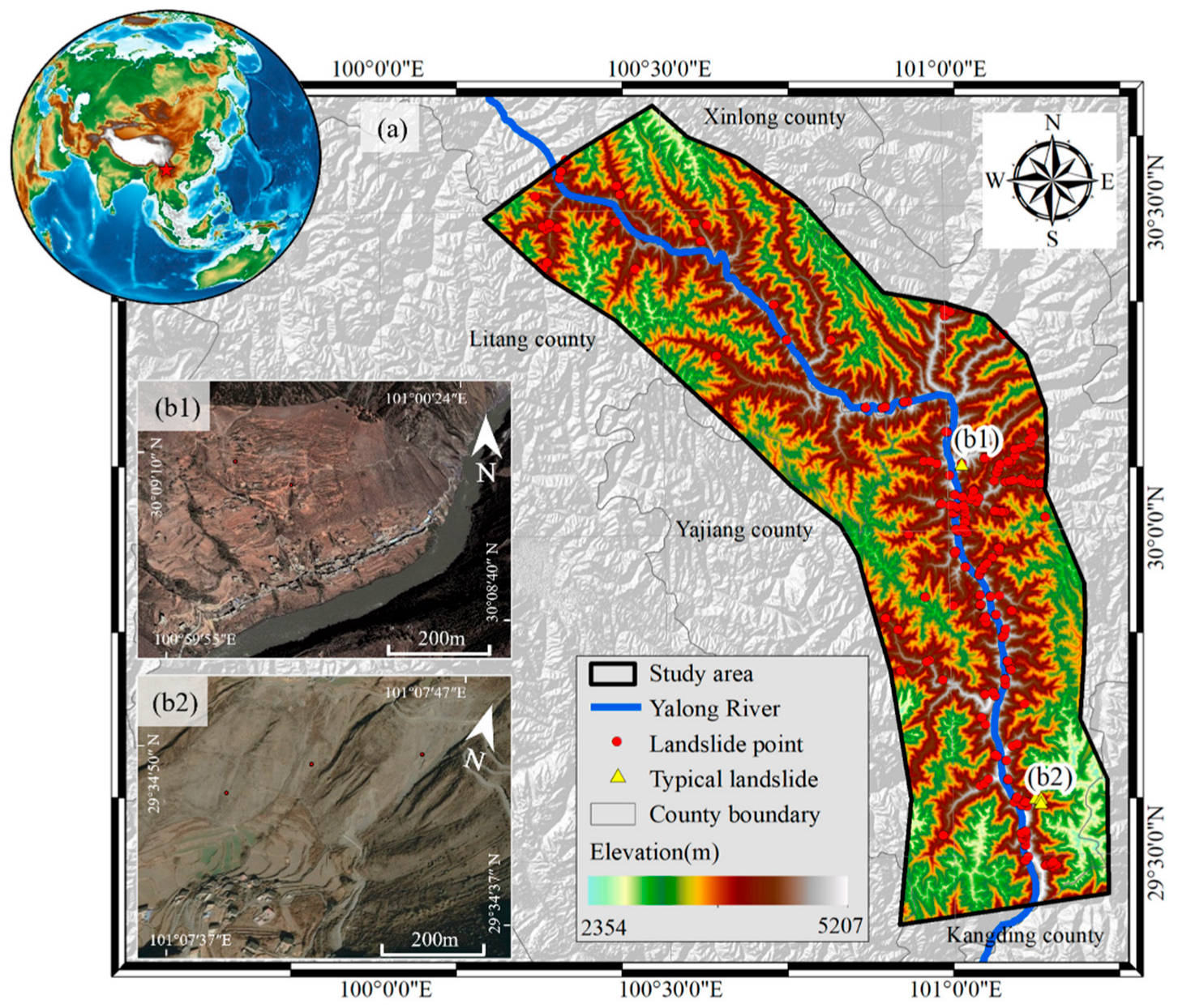
Figure 1. (a) Study area location. (b1,b2) Typical landslide area imagery (Source: Google Earth).
Remotesensing 17 03210 g001
Figure 2. Spatio-temporal baseline plot.
Remotesensing 17 03210 g002
Figure 3. Illustrative maps of the landslide susceptibility factors location of the study. (a) Relief Amplitude. (b) Slope. (c) Aspect. (d) SPI. (e) TWI. (f) Profile Curvature. (g) Plan Curvature. (h) Annual Rainfall. (i) Distance from Faults. (j) Distance from Rivers. (k) Distance from Roads. (l) NDVI. (m) Soil Erosion Types. (n) Lithology. (o) Land Cover. (p) Soil Types. (q) Plant Types. (r) Deformation Velocity.
Remotesensing 17 03210 g003
Figure 4. Technical workflow chart.
Remotesensing 17 03210 g004
Figure 5. Heatmap of Pearson correlation coefficients among evaluation factors.
Remotesensing 17 03210 g005
Figure 6. Multicollinearity analysis of factors (VIF).
Remotesensing 17 03210 g006
Figure 7. Multicollinearity analysis of factors (TOL).
Remotesensing 17 03210 g007
Figure 8. Ranking of landslide susceptibility factors based on factor detector (q-values).
Remotesensing 17 03210 g008
Figure 9. Spatial distribution of SBAS-InSAR-derived surface deformation velocity from May 2020 to May 2023 and associated statistical histogram.
Remotesensing 17 03210 g009
Figure 10. Typical landslide areas derived from SBAS-InSAR analysis. (a) Typical landslide P1. (b) Typical landslide P2. (c) Typical landslide P4. (d) Typical landslide P5. (e) Typical landslide P8. (f) Typical landslide P9. (g) Typical landslide P17. (h) Typical landslide P18. (i) Typical landslide P21. (j) Typical landslide P22. (k) Typical landslide P23. (l) Typical landslide P24.
Remotesensing 17 03210 g010
Figure 11. Hierarchical slope unit partitioning for regional-scale landslide analysis.
Remotesensing 17 03210 g011
Figure 12. Surface deformation velocity within slope units.
Remotesensing 17 03210 g012
Figure 13. Probability distribution in landslide susceptibility prediction: RF vs. RF+ve.
Remotesensing 17 03210 g013
Figure 14. Comparative landslide susceptibility mapping: RF vs. RF+ve.
Remotesensing 17 03210 g014
Figure 15. Stratified distribution of susceptibility units and landslide incidence: RF vs. RF+ve.
Remotesensing 17 03210 g015
Figure 16. (a) ROC curves of two models. (b) Model evaluation metrics comparison.
Remotesensing 17 03210 g016
Figure 17. Comparative Confusion Matrices: RF vs. RF+ve.
Remotesensing 17 03210 g017
Figure 18. SHAP value distribution of the random forest model.
Remotesensing 17 03210 g018
Figure 19. SHAP force plot of representative samples. (a) High-risk sample. (b) Moderate-risk sample. (c) Low-risk sample. (d) Very low-risk sample.
Remotesensing 17 03210 g019
Figure 20. Interaction effects of landslide influencing factors based on geodetector.
Remotesensing 17 03210 g020
Table 1. Main parameters of Sentinel-1 SAR image data.
ParameterSentinel-1 SAR Data
Orbit direction-Track NumberAscending-26
Radar bandC
Radar wavelength (cm)5.6
Spatial resolution (m)20
Incidence angle (°)34.35
Revisit period (days)12
Imaging modeIW
Polarization modeVV
Looks (Range: Azimuth)8:2
Time spanMay 2020–May 2023 (83 Images)
Table 2. Data sources and descriptions.
Data NameResolution/ScaleSource/Data Platform
SRTM DEM30 mNASA Earth data Search
China 1 km Monthly Precipitation Dataset (1901–2023)1 km[56]
National river and road vector data1:250,000National Geographic Information Catalog Service System (Ministry of Water Resources)
1:200,000 Regional Geological Survey Map1:200,000China Geological Survey
ESA World Cover Land Use Dataset10 mESA World Cover Viewer
1:1,000,000 Vegetation Atlas of China1:1,000,000National Glacier and Permafrost Desert Science Data Center
1:1,000,000 Soil Map of the People’s Republic of China1:1,000,000Resources and Environmental Sciences Data Center
Landsat 8 Surface Reflectance Imagery30 mUSGS Earth Explorer
Disclaimer/Publisher’s Note: The statements, opinions and data contained in all publications are solely those of the individual author(s) and contributor(s) and not of MDPI and/or the editor(s). MDPI and/or the editor(s) disclaim responsibility for any injury to people or property resulting from any ideas, methods, instructions or products referred to in the content.