Article

Deep Learning Retrieval and Prediction of Summer Average Near-Surface Air Temperature in China with Vegetation Regionalization

1
College of Natural Resources and Environment, South China Agricultural University, Guangzhou 510642, China
2
Guangdong Academy of Social Sciences, Guangzhou 510635, China
3
Information Centre of Ministry of Natural Resources, Beijing 100812, China
*
Author to whom correspondence should be addressed.
Remote Sens. 2025, 17(18), 3209; https://doi.org/10.3390/rs17183209
Submission received: 25 July 2025 / Revised: 13 September 2025 / Accepted: 15 September 2025 / Published: 17 September 2025

Abstract

Retrieving and predicting summer average near-surface air temperature (SANSAT) across China remain challenging due to the country’s complex topography and heterogeneous vegetation cover. This study proposes an innovative deep learning framework that incorporates vegetation regionalization to achieve high-precision spatiotemporal temperature retrieval and prediction. Using MODIS land surface temperature, vegetation indices, weather station data (2000–2019) and other relevant datasets, we first apply GeoDetector to identify key influencing factors (e.g., nighttime surface temperature, elevation, vegetation index, and population density) within each vegetation region. Based on these findings, we develop a deep neural network (DNN) model, which achieves high accuracy in SANSAT retrieval (with validation R2 ranging from 0.90 to 0.97 and RMSE from 0.46 to 0.64 °C). Results indicate that temperature variations in the eastern monsoon region are primarily influenced by human activity and topography, whereas natural factors dominate in the western regions. Subsequently, using a Long Short-Term Memory (LSTM) network with an optimal seven-year time step, we predict SANSAT for 2020–2023, achieving R2 values of 0.71 in training and 0.69 in testing, which confirms the model’s high reliability in SANSAT prediction. The core innovation of this work lies in its vegetation-regionalized deep learning approach, which explicitly addresses landscape heterogeneity by customizing models to specific eco-climatic zones, thereby quantifying human-nature interactions more effectively than traditional, spatially uniform methods. This framework enhances the understanding of summer temperature dynamics and provides valuable spatial data to support applications in agricultural disaster prevention, ecological conservation, and carbon neutrality. Future research will incorporate multi-seasonal data and enhance the spatiotemporal resolution to further improve NSAT modeling.

1. Introduction

Near-surface air temperature (NSAT) is a critical component of the climate system, directly affecting agricultural productivity, ecosystem stability, urban heat island intensity, and the frequency of extreme weather events [1,2,3,4]. Although monthly mean NSAT predictions provide finer temporal resolution, seasonal averages remain indispensable for both scientific research and practical applications. Seasonal scales can effectively smooth short-term fluctuations, thereby providing more stable indicators of long-term climatic variability. Moreover, many agricultural and ecological processes, such as crop growth cycles, heating and cooling demand, and ecosystem responses, are strongly linked to seasonal rather than monthly thermal conditions. Thus, predicting seasonal mean NSAT offers a robust and policy-relevant perspective for agricultural disaster prevention, ecological conservation, and regional climate adaptation planning. In recent years, the effects of global warming have become increasingly pronounced, with frequent extreme summer weather events in China exerting significant impacts on agriculture and the environment [5,6,7]. High-precision NSAT prediction and spatiotemporal analysis are essential for agricultural disaster mitigation, ecological conservation, and sustainable urban development, and have attracted growing scholarly attention [8,9].
At the regional scale, conventional NSAT retrieval methods typically rely on spatial interpolation of meteorological station observations [10,11,12,13]. However, these methods often fall short in accurately capturing localized NSAT variability in complex geographic environments due to limitations in parameterization schemes and computational capacity [14,15]. Moreover, the wide range of factors influencing NSAT variations—including topography, surface characteristics, vegetation cover type, and human activity intensity—presents substantial challenges for spatial representation. These limitations are particularly pronounced in areas with rugged terrain and sparse station distribution, where traditional station-based interpolation methods exhibit poor spatial representativeness [16,17]. As a result, the ability to effectively analyze spatiotemporal temperature dynamics across heterogeneous regions is severely constrained, posing significant challenges to the accurate estimation of temperature at fine spatial and temporal scales [18,19]. Remote sensing offers key advantages in overcoming these challenges by providing large-scale, high spatial and temporal resolution information, such as land surface temperature (LST) and vegetation indices, which are critical for climate monitoring and environmental assessments [20,21,22]. Currently, MODIS (Moderate Resolution Imaging Spectroradiometer) and similar sensors are widely used for surface temperature monitoring. Their daily coverage has substantially enhanced climate monitoring capacity, making them particularly valuable for large-scale NSAT prediction [21,22,23,24]. Nevertheless, the physical linkage between LST and NSAT is modulated by a variety of factors, such as vegetation canopy structure and atmospheric boundary layer conditions, which complicate efforts to develop generalized conversion models [25,26]. In recent years, machine learning and deep learning approaches have shown substantial promise in improving NSAT retrieval accuracy. Studies have demonstrated that data-driven models—such as multiple linear regression, random forests (RF), and support vector machines (SVM)—can effectively capture the complex relationships among NSAT and its driving factors [27,28]. For high-resolution NSAT predictions, deep learning models, including convolutional neural networks (CNN) and long short-term memory (LSTM) networks, have demonstrated superior performance in extracting spatiotemporal features [29]. However, due to China’s vast geographic extent and climatic heterogeneity, NSAT dynamics exhibit strong regional variation [30,31]. This necessitates the development of region-specific prediction models tailored to different ecological zones and vegetation types in order to enhance model applicability and forecasting accuracy. In particular, traditional spatial interpolation methods (e.g., spline, kriging) often show limited accuracy across different regions of China: in western mountainous areas, sparse station distribution and complex topography reduce their effectiveness, whereas in the rapidly urbanizing eastern plains, they may fail to capture the impacts of land use change and human activities on temperature patterns. These regional deficiencies further highlight the necessity of developing a nationwide, regionally adaptive modeling framework.
Thus, a vegetation-type-based regional framework was adopted to explore the spatiotemporal dynamics of summer average near-surface air temperature (SANSAT) across China in this study. By integrating multi-source remote sensing and geographic data, we employed the Geographical Detector model to identify optimal temperature-related indicators within different vegetation regions. Deep learning models were subsequently introduced to retrieve SANSAT distributions for the period 2000–2019. Furthermore, an LSTM-based forecasting model was developed to predict SANSAT from 2020 to 2023.

2. Materials and Methods

2.1. Study Area

China is located in the eastern part of Asia (73°33′E to 135°05′E and 3°51′N to 53°33′N) and covers approximately 9.6 million km2. Its vast territory, complex terrain, and diverse climate contribute to the formation of distinct vegetation distribution patterns (Figure 1). Based on vegetation types, China can be divided into several ecological regions, ranging from evergreen broad-leaved forests along the southeastern coast to desert vegetation in the arid northwest. The temperature variations in each region are not only regulated by regional climate but also influenced by underlying surface characteristics. Different vegetation types play a key role in the NSAT feedback mechanisms [32,33].
China’s summer climate is primarily influenced by the East Asian monsoon system. Water vapor transported by the monsoon decreases from the southeastern coast to the northwestern interior, creating a significant gradient in NSAT distribution across regions [34,35]. Additionally, the Tibetan Plateau, with an average elevation exceeding 4000 m, plays a crucial role in modulating atmospheric circulation, further shaping the NSAT distribution across the country [36,37]. Given the critical role of NSAT in agriculture and ecosystems, investigating its spatiotemporal characteristics and the regulatory effects of vegetation can improve our understanding of climate change impacts and provide scientific support for agricultural planning and environmental management.

2.2. Data

2.2.1. Satellite Data

Satellite remote sensing provides a valuable source of information for SANSAT retrieval and prediction by utilizing multiple spectral bands to monitor changes in climate-related indicators, thereby indirectly capturing the dynamics of NSAT [38,39,40]. The remote sensing datasets used in this study primarily include MODIS products, digital elevation models (DEMs), and soil moisture data. As detailed in Table 1, the surface temperature (MOD11A1), vegetation index (MOD13A2), and surface albedo (MCD43A3) from June to August during 2000–2019, and elevation imagery were collected from Google Earth Engine (GEE, https://earthengine.google.com (accessed on 1 July 2024)).

2.2.2. Meteorological Data

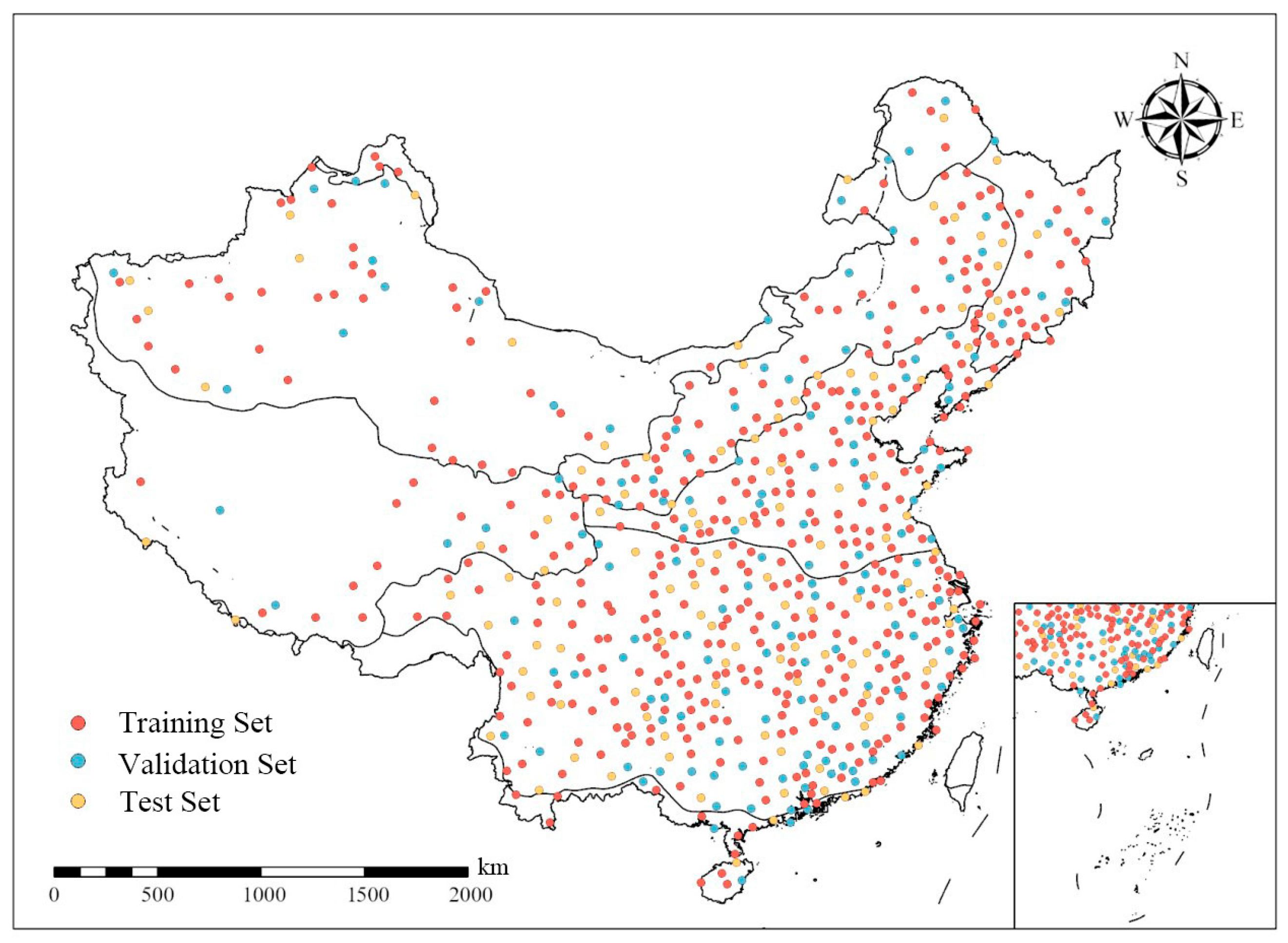
The sample data of this study were mainly obtained from the daily ground climate dataset provided by the National Meteorological Science Data Center of China (http://data.cma.cn/ (accessed on 10 July 2024)). Based on meteorological observations—including summer average air temperature, sunshine duration, relative humidity, wind speed, barometric pressure, and other parameters—collected from 709 national meteorological stations between 2000 and 2019, the sample points were divided into three groups using stratified sampling across eight vegetation regions (Figure 2). The samples followed an approximate 3:1:1 ratio, maximizing training data while preserving independent subsets for model tuning and unbiased evaluation. Red samples were used to train the SANSAT retrieval and prediction model, blue samples were used for model validation, and yellow samples were used to verify the mapping accuracy. The detailed distribution of sample points is presented in Table 2. The data represent summer averages from June to August during the period 2000–2019, with 20 samples collected for each sample point. The cold-temperate coniferous forest region had the fewest training samples, with only four sample points and 80 training records. Although a sample size above 50 meets the minimum requirements for statistical modeling, cross-validation was employed in this region due to the limited number of validation samples.

2.2.3. Geographic Data

The geographic datasets used in this study primarily include population density and vegetation zoning data for China. Population density data were obtained from the WorldPop dataset (https://www.worldpop.org/ (accessed on 10 July 2024)), which provides gridded population data for China at the kilometer scale. This dataset integrates multiple sources—including land use and nighttime light intensity—to estimate population distribution at a spatial resolution of 100 m, offering a quantitative representation of population spatial patterns and human activity intensity.
Vegetation region data were obtained from the 1:1,000,000 Vegetation Atlas of China, compiled by the Institute of Botany, Chinese Academy of Sciences, and edited by Ke-Lin Hu. The dataset was published in 2001 and is available through the Resource and Environment Science Data Center (https://www.resdc.cn/ (accessed on 10 June 2024)). The regional classification is based on eco-climatic factors (e.g., mean temperature of the warmest and coldest months, precipitation, aridity index) and geomorphological units (e.g., mountain systems, plateau boundaries), dividing the country into eight vegetation regions (I–VIII). The boundaries of these regions closely align with climatic zones and vegetation distribution patterns, providing a standardized environmental framework that effectively supports the analysis of temperature variations across different vegetation–climate regions.

2.3. Data Processing

In this study, MODIS products (e.g., MOD11A1, MOD13A2, MCD43A3) acquired from the Google Earth Engine (GEE) platform had already been preprocessed by NASA, including atmospheric correction, radiometric correction, and orthorectification. Subsequent processing involved cloud removal using the C Function of Mask (CFMASK) algorithm, combined with QA bands to enhance cloud detection accuracy [41,42,43]. The preprocessed products were then converted to appropriate units, clipped to the study area, and aggregated into seasonal mean values (June–August) for each year from 2000 to 2019, ensuring that all datasets consistently represent summer averages. Subsequently, remote sensing indices were calculated. Using bilinear interpolation, the remote sensing and population density datasets were resampled to a spatial resolution of 1000 m and projected to the WGS 84 geographic coordinate system.
In addition, to ensure the integrity of meteorological data and the reliability of the analysis, stations with missing data for three years or more were excluded based on predefined rejection criteria. As a result, 709 meteorological stations were retained, providing key climate variables such as temperature, sunshine duration, relative humidity, wind speed, and air pressure. Average values of each variable from June to August were calculated, and their spatial distributions were generated via interpolation using ANUSPLIN (version 4.4, Canberra, Australia) software.

2.4. Methods

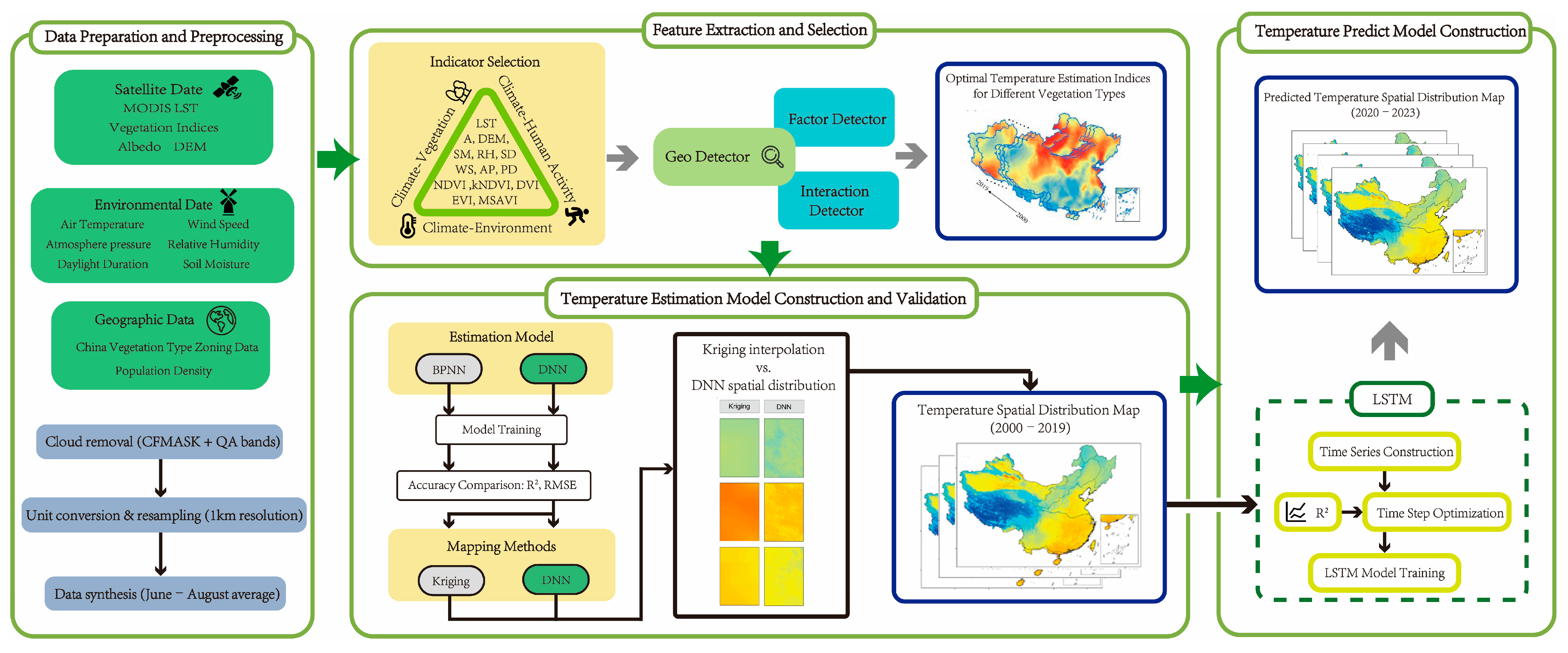
The overall workflow of this study is presented in Figure 3. The first step involved acquiring the required datasets and performing band calculations on the selected remote sensing products. Next, the Geodetector method was applied to select the best SANSAT retrieval indicators for different vegetation regions, and deep neural networks (DNN) and backpropagation neural networks (BPNN) models were developed to construct the SANSAT retrieval model. Finally, the Long Short-Term Memory (LSTM) algorithm was employed to predict SANSAT based on time-series data.

2.4.1. Extraction of SANSAT Retrieval Indicators

In this study, we explored the relationship between climate and temperature from three perspectives: climate–environment, climate–human activity, and climate–vegetation. Relevant indicators were selected accordingly based on these dimensions [44,45]. Specifically, surface temperature (LST_Day, LST_Night), surface albedo (SA), elevation (DEM), atmospheric relative humidity (RH), sunshine duration (SH), wind speed (WS), barometric pressure (PRS), and soil moisture (SM) were chosen to represent the climate–environment dimension. Population density (PD) was selected for the climate–human activity dimension. Vegetation indices, including NDVI, KNDVI, DVI, EVI, and MSAVI, were employed to characterize the climate–vegetation relationship [46,47]. Among these, variables such as surface temperature, elevation, population density, and soil moisture were directly obtained from preprocessed products. The remaining indicators were calculated using standard formulas, as detailed below:
(1)
Surface Albedo (SA)
Surface albedo is defined as the ratio of solar radiation reflected from the Earth’s surface to incident solar radiation [48,49], and is widely used in studies of the land surface energy balance, weather forecasting, and climate change [50]. The MODIS surface albedo product MAD43A3 provides two types of albedo estimates: Black-Sky Albedo (BSA), representing albedo under purely direct solar illumination, and White-Sky Albedo (WSA), representing albedo under entirely diffuse conditions. The real surface albedo is typically computed as a weighted linear combination of BSA and WSA based on the prevailing diffuse light fraction in the atmosphere [51,52], as shown in Equation (1).
α = α W S A × r + α B S A × 1 r
where α is the real surface albedo; α WSA is the white sky albedo; α BSA is the black sky albedo; and r is the proportion of the actual sky diffuse light, which can be obtained from the empirical statistical relationship [48] for the clear-sky conditions (Equation (2)).
r =   0.122 + 0.85 × e x p 0.48 c o s θ
where θ is the zenith angle of the sun at noon; cos θ is the cosine of the zenith angle of the sun at noon.
(2)
Normalized Difference Vegetation Index (NDVI)
NDVI is a standardized index, which is widely used to detect vegetation growth and vegetation coverage, and can better reflect the special spectral characteristics of vegetation [53,54,55], and can be used to monitor vegetation growth, s. Introducing the NDVI, Equation (3) can be written as:
N D V I =   N I R R / N I R + R
where NIR is the near-infrared band and R is the infrared band. The range of NDVI is [−1, 1].
(3)
Kernel Normalized Difference Vegetation Index (KNDVI)
Compared with NDVI, KNDVI can better deal with noise, complex climatic and background effects (e.g., bare soil, water, snow, etc.). Under various environmental conditions, such as grassland, farmland, mixed forest, and arid areas, this index can make maximum use of spectral information, showing better stability and robustness than the traditional index [56,57,58]. It can be calculated as follows:
K N D V I =   t a n h   N I R R 2 σ 2
where NIR denotes the near-infrared band, R represents the infrared band, and σ signifies a scale parameter indicating the sensitivity of the index to sparsely/intensely vegetated areas. It is customary to average σ as σ = 0.5 × NIR R .
(4)
Difference Vegetation Index (DVI)
DVI is capable of detecting vegetation growth status, vegetation cover, and eliminating some of the radiometric errors, etc. It is sensitive to changes in the soil background and can better recognize vegetation and water bodies [59,60] and can be expressed as follows:
D V I =   N I R R
where NIR is the near-infrared band, R is the infrared band, and DVI falls within the range of [−1, 1].
(5)
Enhanced vegetation index (EVI)
EVI is an optimized vegetation index [61,62]. It has been shown to significantly improve vegetation monitoring by adding blue band B2 to enhance the vegetation signal, thereby reducing the effects of soil background and aerosol scattering on the vegetation index and improving the biomass regional sensitivity (Equation (6)).
E V I =   2.5 × N I R R N I R + 6 R 7.5 B + 1
where NIR is the near-infrared band, R is the infrared band, B is the blue band. EVI is in the range [−1, 1].
(6)
Modified Soil Adjusted Vegetation Index (MSAVI)
MSAVI was developed to reduce the influence of soil background in vegetation monitoring and is particularly effective in areas with high bare soil exposure, sparse vegetation cover, or low chlorophyll content [63,64]. It serves as a refinement to the NDVI, which may fail to produce reliable estimates under such conditions. The calculation is as follows:
M S A V I =   1 2 2 N I R + 1 2 N I R + 1 2 8 N I R R
where NIR is the near-infrared band, R is the infrared band.

2.4.2. Selection of Optimal Indicators for SANSAT Retrieval

Geographical detectors (Geodectors) are a set of statistical methods to detect spatial heterogeneity and reveal the driving forces behind it, which mainly include factor detectors, interactive detectors, risk detectors, and ecological detectors. As a spatial statistical technique operating within an analysis of variance (ANOVA) framework, GeoDetector excels at identifying key drivers influencing the spatial heterogeneity of dependent variables. A significant advantage is its non-parametric nature; it does not require prior assumptions of linear relationships between variables. This feature allows it to effectively avoid issues of multicollinearity among explanatory variables and overcome the limitations traditional methods face when analyzing categorical variables, as it imposes minimal model assumptions [65,66]. Given its strengths, this study mainly uses a factor detector and an interactive detector to determine the retrieval indicators of SANSAT.
The factor detector is utilized to assess the explanatory power of individual factors on the spatial distribution of SANSAT. This is quantified using the q-statistic, which measures the proportion of the total variance of a dependent variable that can be explained by a given factor. The q-value is derived from Equation (8):
q =   1 i = 1 L N i × σ i 2 N × σ 2 = 1 S S W S S T
where L represents the stratification of variables or influencing factors, which refers to the classification or partitioning of spatial units; N i and N are the number of units in the i-th stratum and the whole region, respectively; σ i 2 and σ 2 indicate the variance of the dependent variable within the i-th stratum and across the whole region; SST is the sum of intra-layer variance; SST is the range of total variance. q in the whole region [0, 1]. In this study, the larger the q value, the greater the influence of the factor on the SANSAT.
The interaction detector is applied to assess the combined influence of two factors X 1 and X 2 , on near-surface air temperature, and to determine whether their joint effect strengthens or weakens spatial heterogeneity compared to their individual contributions [67,68]. The main results of this study include nonlinear attenuation, one-factor nonlinear attenuation, two-factor enhancement, independent and nonlinear enhancement, as shown in Table 3.

2.4.3. Model Construction for SANSAT Retrieval

To obtain the optimal retrieval model for near-surface air temperature, we employed DNN and BPNN models based on the optimal temperature retrieval indicators identified in Section 3.2. These models were used to characterize the relationships between the selected response indicators and near-surface air temperature. By comparing the performance of both models, the most accurate and suitable SANSAT retrieval model was determined, thereby enhancing the reliability and applicability of remote-sensing-based temperature monitoring.
(1)
DNN model
The Deep Neural Network (DNN) is a classical deep learning model known for its superior performance in handling large and complex datasets. Compared with shallow neural networks, DNNs exhibit stronger nonlinear fitting capabilities and are adept at capturing hidden relationships among environmental variables [69]. In this study, a Deep Neural Network (DNN) model was introduced to construct the mapping relationship between remote sensing and geographical factors and SANAST. The model consists of an input layer, multiple hidden layers, and an output layer, all fully connected, as illustrated in Figure 4. Specifically, the network topology is defined as x–128–128–128–128–1, where x represents the number of optimal explanatory variables selected for each vegetation region. Each of the four hidden layers contains 128 neurons, and the output layer has a single node corresponding to the retrieved SANAST value.
To prevent overfitting, the model incorporates dropout regularization, with a dropout rate of 0.1, meaning that each neuron has a 10% probability of being randomly deactivated during training. Each hidden layer uses the ReLU (Rectified Linear Unit) activation function to capture nonlinear relationships, while the output layer uses a linear activation function, which is suitable for continuous regression output. This configuration improves the model’s robustness and generalization capability.
(2)
BPNN model
BPNN is a widely adopted artificial neural network architecture, particularly effective for tasks such as classification and regression [70]. As a supervised learning approach, BPNN iteratively minimizes prediction errors by adjusting the network’s weights through error backpropagation [71,72]. Structurally, BPNN follows a feedforward framework composed of an input layer, one or more hidden layers, and an output layer. Its fundamental principle is to minimize overall model error by continuously updating the connection weights. This is achieved by propagating the output error backward through the network and adjusting the weights of hidden neurons to better approximate the target output [73]. The typical architecture of a BPNN used in this study is illustrated in Figure 5. It serves to capture the complex nonlinear relationships between input indicators and near-surface air temperature, thereby enhancing the robustness and accuracy of remote sensing-based temperature retrieval.

2.4.4. Model Construction for SANAST Prediction

LSTM is a specially designed recurrent neural network (RNN) architecture that dynamically regulates the information flow by introducing gating mechanisms (input gate, forgetting gate, and output gate), effectively solves the long-term dependence problem of traditional RNN due to gradient vanishing/exploding, and shows excellent temporal correlation modeling ability in the field of time series forecasting [74,75]. Therefore, the LSTM model is employed in this study to predict the SANAST based on the retrieval data of SANAST from 2000 to 2019, as shown in Equation (9):
h t =   ο t × t a n h C t
where ht is the predicted SANAST value of time t, t is every year from 2000 to 2019, Ct is the SANAST information of time t, ο t is the output gate of time t, and t a n h is the output function. The calculation of ο t and ο t is as follows:
ο t =   S i g m o d W ο x t + W ο h t 1 + W ο C t 1 + b ο
C t = f t × C t 1 + i t × t a n h W C x t + W C h t 1 + b C
where x t represents the input variable at time t ; W and b denote the weights and biases, respectively; and Sigmod is the activation function; The input gate i t and forget gate f t are computed as i t =   Sigmod W i x t + W i h t 1 + W i C t 1 + b i and f t =   Sigmod   W f x t + W f h t 1 + W f C t 1 + b f . Figure 6 illustrates the architecture of the LSTM model.

2.4.5. Model Accuracy Verification

To evaluate model performance, this study employed three widely used statistical metrics: the coefficient of determination (R2), bias, and root mean square error (RMSE) [76,77]. The R2 value represents the proportion of variance in the observed SANAST data explained by the model, providing a measure of its explanatory power and overall stability (Equation (12)). Bias is defined as the arithmetic mean of the prediction errors, indicating the model’s systematic deviation from the observations (Equation (13)). While it offers an overall indication of model bias, its main limitation is the potential offset between positive and negative errors, which may underestimate the true magnitude of prediction errors. In contrast, RMSE measures the average magnitude of prediction errors in absolute terms by taking the square root of the mean squared differences between predicted and observed values, thereby serving as a robust indicator of model accuracy (Equation (14)).
R 2 = i = 1 n y ^ i y ¯ 2 / i = 1 n y i y ¯ 2
b i a s =   i = 1 n y ^ i y i / n
R M S E =   i = 1 n y i y ^ i 2 / n
where y i is the measured SANAST of the i-th sample, y ^ i is the predicted SANAST value of the i-th sample, y ¯ is the mean of the measured values, and n is the number of samples. The smaller the Bias and RMSE values, the closer the R2 value is to 1, which means that the model has higher accuracy; conversely, the larger the Bias and RMSE values, the smaller the R2 value, indicating the lower the accuracy of the model.

3. Results

3.1. Selection of the Optimal Indicators for SANAST Retrieval

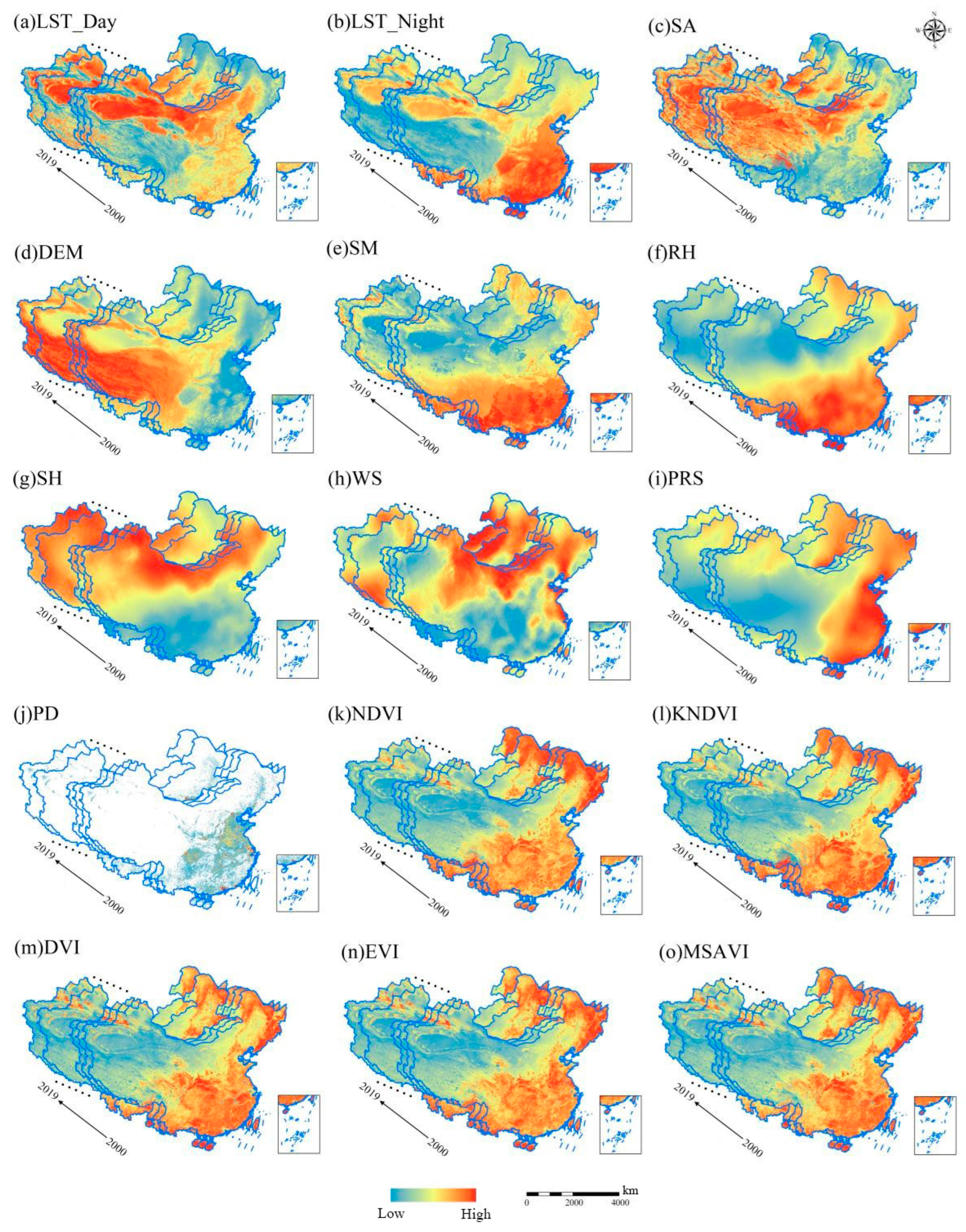
In this study, the spatial distributions of 15 SANAST retrieval indicators, including NDVI and KNDVI, were derived for the period 2000–2019 following the methodology described above (Figure 7).
As shown in Figure 7, the LST is higher in the northwestern and eastern regions; however, in the temperate desert region—particularly the Taklimakan Desert—it is markedly higher than in other areas, with a pronounced diurnal temperature range primarily attributable to the synergistic influence of the low heat capacity of surface materials and the prevailing arid climatic conditions. SA exhibits marked spatial heterogeneity, with higher values concentrated in the alpine vegetation region (often snow-covered), temperate grasslands, and desert regions characterized by sparse vegetation. In contrast, localized low SA values are observed in the semi-arid transitional zones, likely due to variations in soil roughness and moisture content.
The DEM exhibits a west-high-east-low pattern, accompanied by substantial spatial coupling with the SM and RH. The high-value zones of the SM and RH are predominantly located in the precipitation-rich southern monsoon region, with secondary concentrations extending into the frigid coniferous forest belt. WS forms a dual-core distribution in the northwest inland and coastal areas, which is driven by westerly jet intensity and land–sea thermal gradient, respectively. High PRS values are concentrated in the densely populated eastern coastal region, suggesting that urbanization may modulate local pressure fields through the urban heat island effect. Vegetation indices (NDVI, KNDVI, DVI, EVI, and MSAVI) exhibit a pronounced latitudinal zonality. High vegetation index values extend from tropical monsoon rainforests to cold-temperate coniferous forests, whereas low values are concentrated in temperate desert and alpine vegetation regions, where water and thermal resources are limited. Overall, the spatial distribution patterns of all environmental parameters are consistent with the general law of land surface environmental differentiation across China.
Subsequently, the factor detector and interaction detector within the Geographical Detector framework were applied to quantify the influence of various environmental indicators on regional air temperature. In this analysis, SANAST values for each vegetation region served as the dependent variable (Y), while the 15 aforementioned indicators were used as independent variables (X). This approach facilitated the identification of key drivers for SANAST retrieval across different vegetation regions.
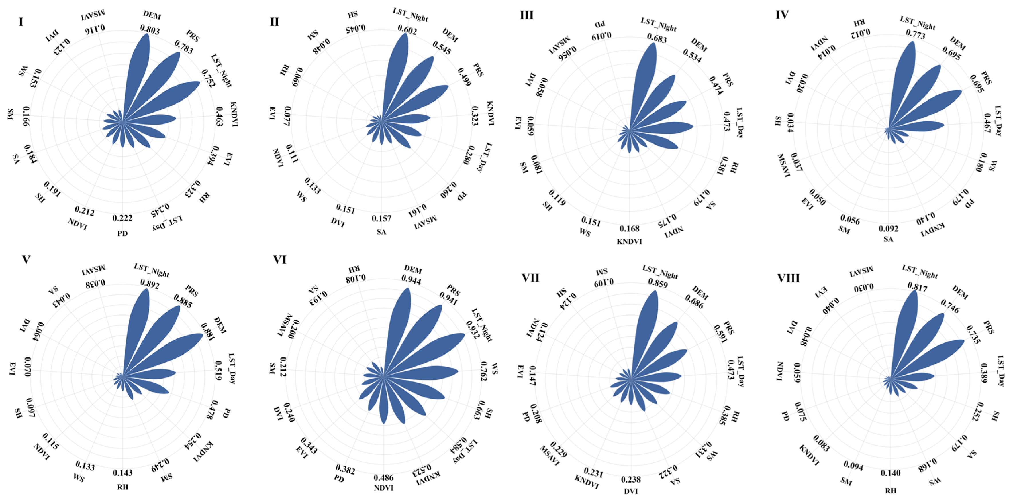
Results from the factor detector analysis (Figure 8) indicate that LST_Night, DEM, and PRS are the dominant factors influencing temperature variation across vegetation regions. When these core variables interact with other indicators, they exhibit a synergistic enhancement effect that further amplifies their influence on regional SANAST dynamics. Notably, the influence of human activity intensity on SANAST change varies significantly across regions. Human activities and associated land use changes directly affect energy conversion in densely populated areas, resulting in different drivers of SANAST change across regions. The eastern regions (I, II, IV, V, and VI) feature flat topography, a favorable climate, much higher population density than that in the western regions, and have formed stable urban clusters. In these regions, the combined influence of human activity intensity and topographic factors has a particularly significant effect on SANAST. Conversely, in the western regions (III, VII, and VIII), which primarily include the Tibetan Plateau and the non-monsoon zones, temperature variation is predominantly governed by natural factors. These areas are marked by sparse vegetation, low population density, and minimal anthropogenic disturbance.
Furthermore, in regions with dense vegetation cover (e.g., I, II, V, VI, and VII), vegetation indices contribute over 20% to temperature variability. In contrast, in the temperate desert region (VIII), the contribution rate is less than 10%, indicating a greater influence of other environmental indicators. Through their complex and spatially variable interactions, these dominant driving factors collectively shape distinct patterns of spatiotemporal differentiation in regional SANAST dynamics across diverse vegetation types.
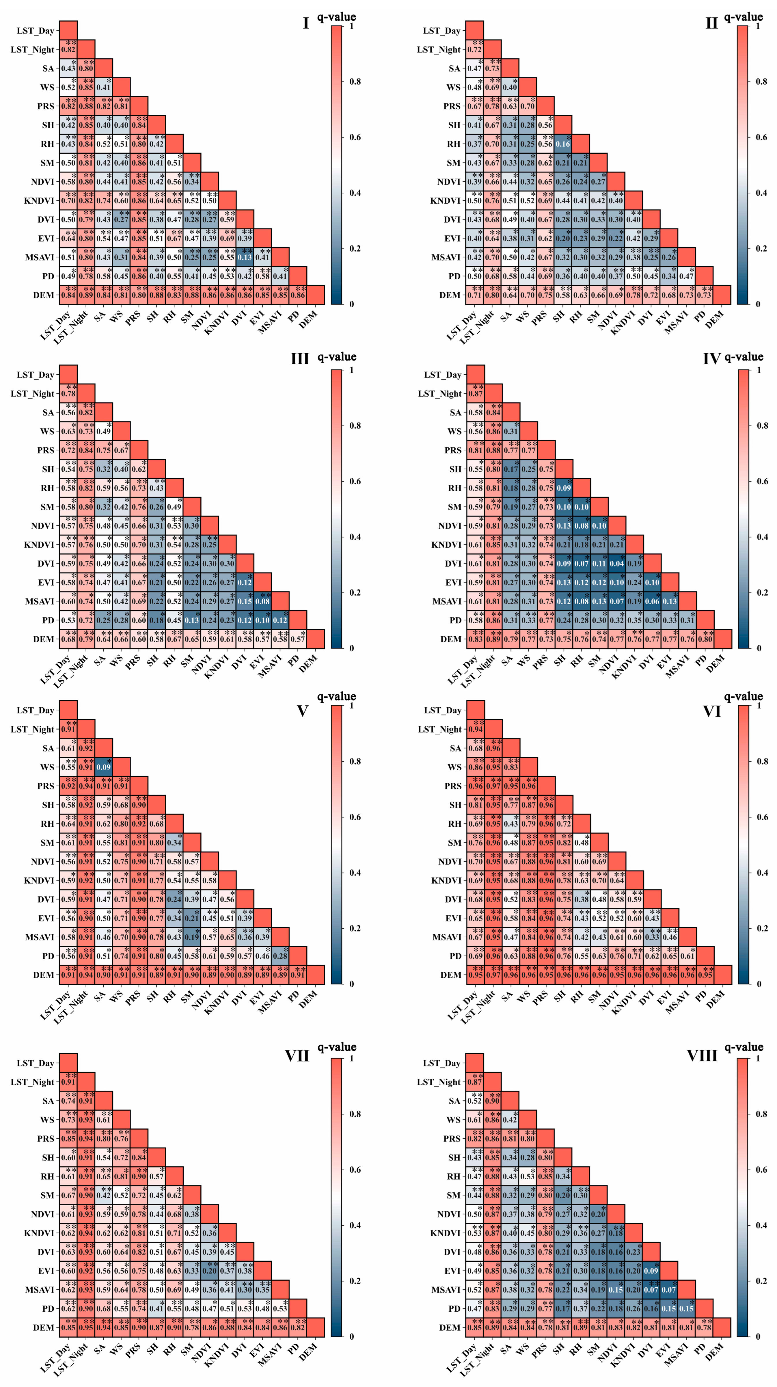
The interaction detector measures the difference between the q-values of individual factors and those of factor pairs, thereby elucidating both the nature and magnitude of interactions among influencing factors across different vegetation and climate regions. It also examines the regional variability of SANAST changes driven by the combined effects of multiple factors. To capture these spatial variations, the indicator values were evaluated separately for each vegetation region (Figure 9).
As shown in Figure 9, most variables within each vegetation region exhibit strong two-factor and nonlinear enhancement effects. For instance, in the cold temperate coniferous forest region (I), LST_Day exhibits a two-factor enhancement pattern when interacting with natural variables such as DEM, EVI, KNDVI, RH, SH, PRS, and LST_Night, and shows nonlinear enhancement when combined with anthropogenic indicators such as PD, MSAVI, DVI, NDVI, SM, WS, and SA. Although the individual contributions of DVI and MSAVI are low, their synergistic interaction substantially enhances their overall influence. The superposition of anthropogenic factors also greatly enhances the effects of other factors on SANAST alone, so population density can be used as an auxiliary indicator for the study of anthropogenic impacts. In summary, at the current stage, temperature variations across different vegetation regions in China exhibit significant spatial heterogeneity, driven by the combined influence of multiple factors. Among these, topographic factors—such as elevation lapse rates and slope orientation—serve as relatively stable drivers that directly affect air temperature, while the continuous presence of mountain ranges further increases the complexity of regional climate patterns.
In addition, key natural factors, including sunshine duration and vegetation cover, primarily regulate near-surface air temperature by modulating solar radiation input. These factors have broad spatial influence, persistent effects, and relative stability; despite interannual fluctuations, their energy gains and losses tend to offset each other over time. Furthermore, in the eastern regions, human activities radiate outward from urban centers, exerting a measurable yet spatially limited impact. Overall, temperature changes across China’s diverse regions are shaped by the intertwined effects of natural and anthropogenic factors, resulting in complex and uncertain spatiotemporal patterns. To optimize the input variables for SANAST retrieval in each vegetation region, this study selected variables with a single-factor contribution exceeding 15% and the highest q-value in interaction tests. These selected variables were incorporated into the SANAST retrieval model after multiple rounds of validation, and the final results are presented in Table 4.

3.2. Optimized SANAST Retrieval Model

To develop the most effective SANAST retrieval model, this study used a dataset comprising 435 training samples. The selected SANAST retrieval indicators for each vegetation region (Table 4) were treated as independent variables, while corresponding SANAST observations served as dependent variables. Relationship models between the indicators of various vegetation types and SANAST were constructed using both BPNN and DNN models, with algorithm parameters optimized based on experimental data. Finally, the retrieval accuracy of the two models was compared.
As shown in Figure 10, the BPNN model achieved R2 values exceeding 0.80 across all vegetation regions, with RMSE values ranging from 0.71 °C to 1.46 °C. In contrast, the DNN model demonstrated superior performance, achieving R2 values exceeding 0.9 and RMSE values below 0.5 °C for all vegetation regions. These results indicate that the DNN model offers more accurate and stable retrieval of SANAST.
To further validate model robustness, performance was assessed on an independent test dataset, and the results are illustrated in Figure 11. The DNN model continued to outperform the BPNN model in both R2 and RMSE metrics, mirroring the training set performance. This consistency suggests that the DNN model is not affected by overfitting and possesses strong generalizability in air temperature retrieval tasks.
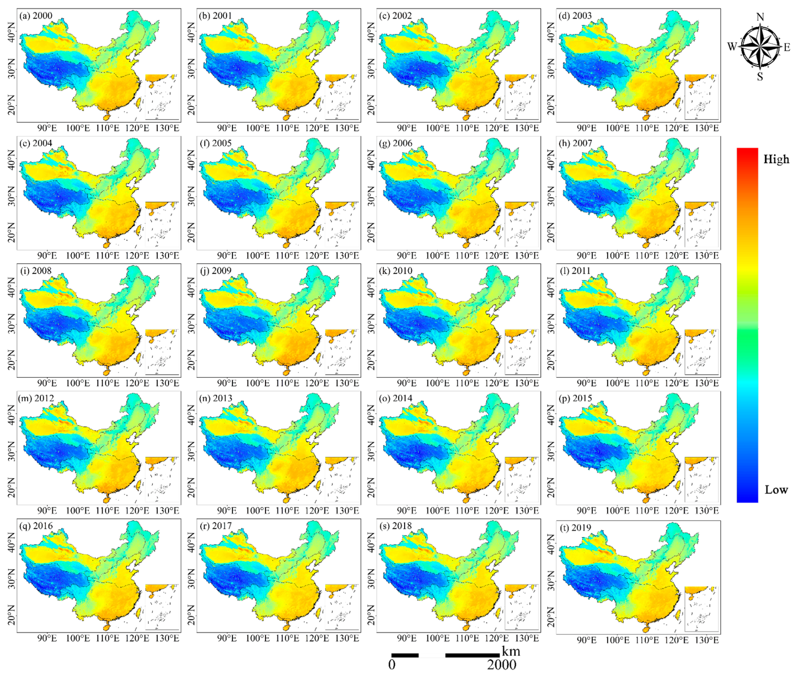
Therefore, the DNN model was identified as the best SANAST retrieval model in this study. To further verify the reliability of the model, the spatial distribution of summer mean SANAST in China from 2000 to 2019 was obtained by using the DNN model with the SANAST retrieval indicators of each vegetation type area. As shown in Figure 12, the SANAST distribution of China generally presents a pattern of ‘high in the southeast coastal areas and northwest arid areas, low in the northeast and Qinghai–Tibet Plateau’ and decreases with the increase in latitude, which is mainly controlled by solar radiation. Southeast urban agglomerations (Yangtze River Delta, Beijing–Tianjin–Hebei, and Pearl River Delta) are high SANAST centers, which may be affected by urbanization and greenhouse gas emissions. The high SANAST in the Taklimakan Desert reflects the unique climate characteristics of the region. The low SANAST centers are mainly distributed in the alpine vegetation region of the plateau (VII). The SANAST in the Qinghai–Tibet Plateau is significantly lower than that in the eastern part of the same latitude, which is significantly affected by altitude. Overall, solar radiation determines the macro pattern, and altitude and underlying surface characteristics shape regional SANAST heterogeneity.
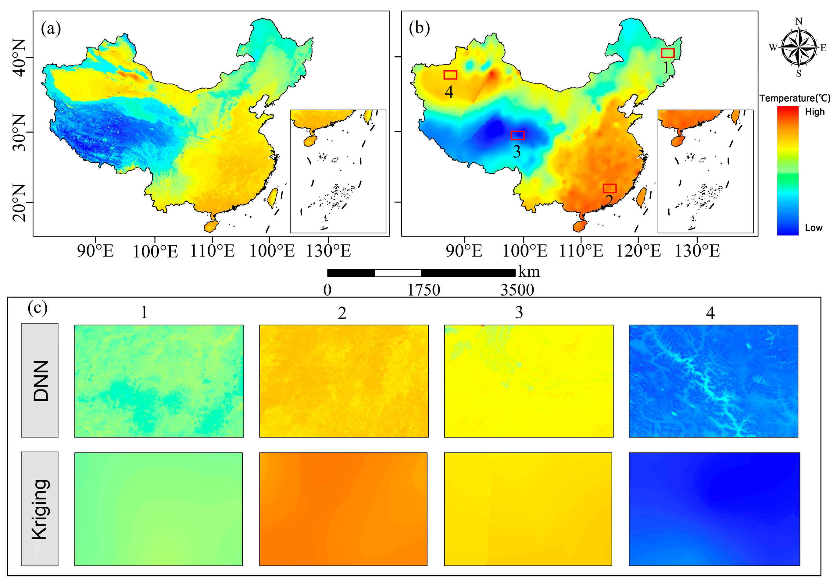
Moreover, this study validated the mapping accuracy of the SANAST spatial distribution from 2000 to 2019 using 130 independent validation samples (Figure 13). The results showed that the DNN model achieved an R2 of 0.95, a bias of 0.16 °C, and an RMSE of 1.20 °C, indicating its strong capability to accurately estimate the national SANAST and its good generalizability. As illustrated in Figure 14, taking the SANAST in 2018 as an example, the DNN-derived spatial distribution map provides more detailed regional-scale features compared with the kriging interpolation method, thereby better capturing the spatial heterogeneity and improving the representation accuracy of SANAST data.

3.3. Optimized SANAST Prediction Model

Based on the SANAST retrieval data obtained in the previous section, this study further constructs a deep learning model to enhance the SANAST prediction capability. Initially, a spatially uniform sampling approach using the fishing net method was adopted, and outliers with large errors were removed, resulting in a total of 25,000 valid sample points. For these sample points, SANAST estimates from 2000 to 2019 were extracted, and the dataset was partitioned into training and testing subsets in a 7:3 ratio. Subsequently, the LSTM algorithm was employed to construct the SANAST prediction model.
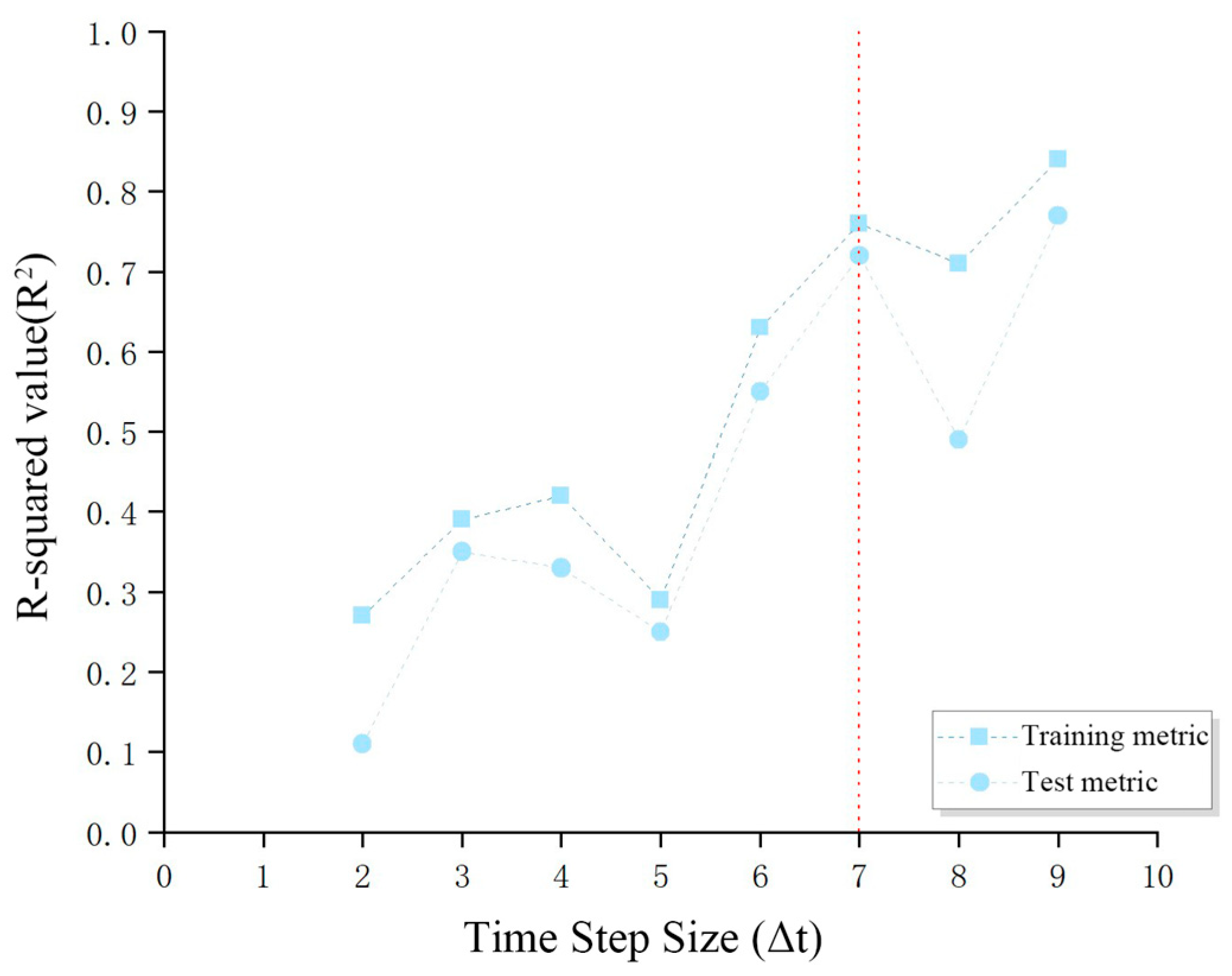
To identify the optimal temporal step length for the LSTM model, nine schemes with varying step lengths were designed and systematically evaluated. As shown in Figure 15, when the step length was less than 7 years, the model exhibited reduced prediction stability and lower accuracy. In contrast, step lengths greater than 7 years tended to cause overfitting and impair generalization capability. Considering both accuracy and stability, a step length of 7 years was identified as optimal, as it minimized errors in both the training and testing sets.
After determining the optimal time step, the model parameters were further fine-tuned through a series of experimental trials. Specifically, the LSTM model was trained using SANAST time-series data from 2000 to 2019 as input, employing a rolling window of 7 years (i.e., the previous seven consecutive years of SANSAT) to predict the temperature of the subsequent summer. For example, data from 2000 to 2006 were used to predict 2007, data from 2001 to 2007 to predict 2008, and so forth, ensuring that each training sample incorporated sufficient historical context.
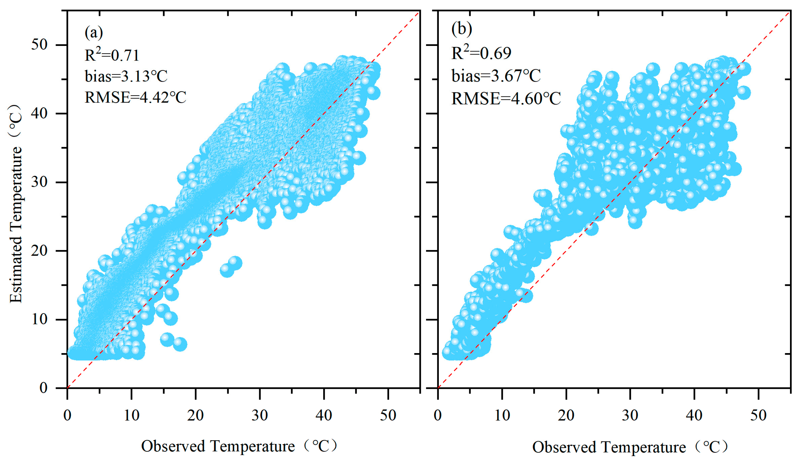
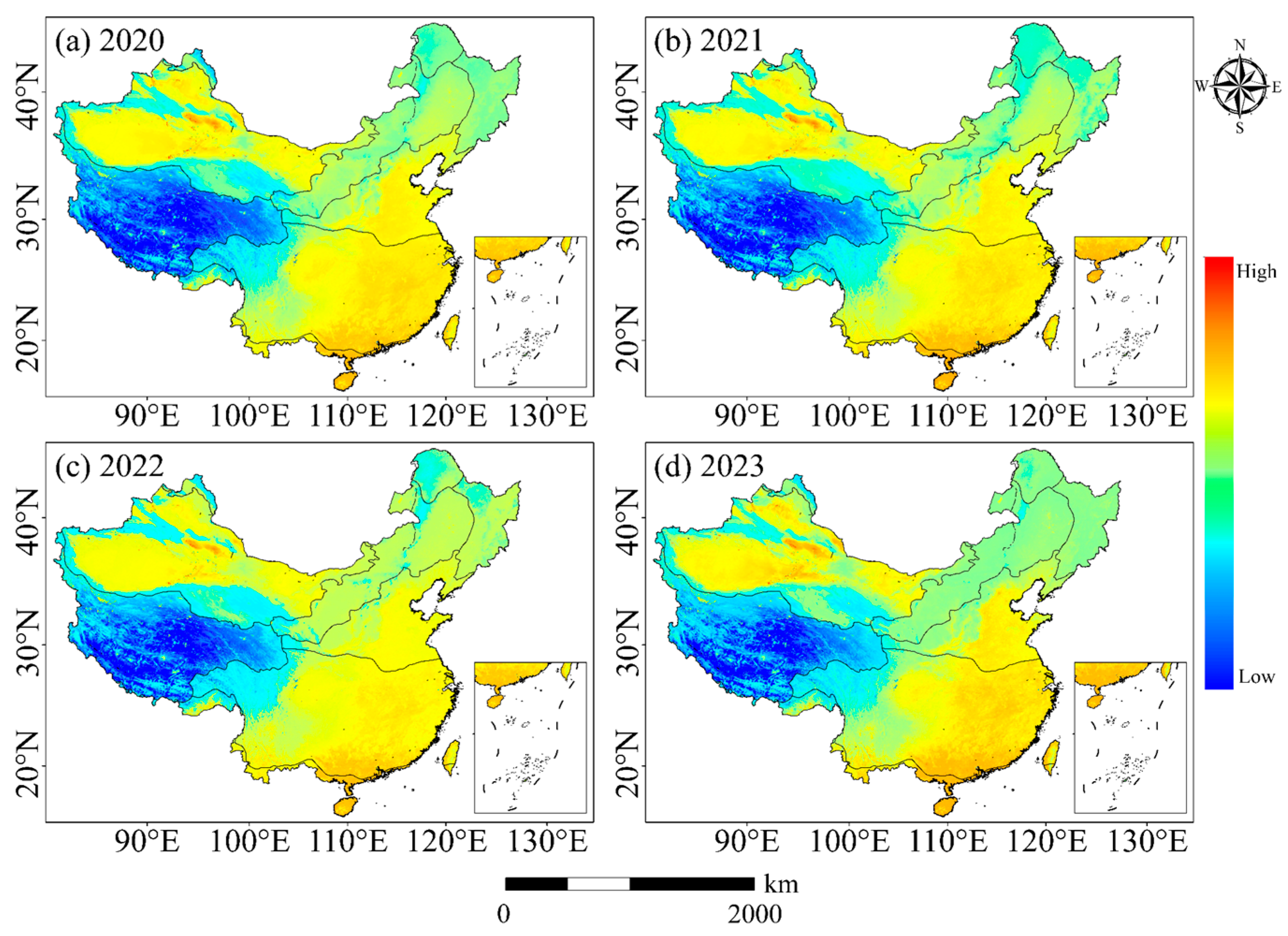
The final LSTM model configuration consisted of 50 hidden units and 200 training iterations, ensuring robustness and generalizability for complex time-series data. As shown in Figure 16, the optimized model achieved R2 values of 0.71 (training) and 0.69 (testing), with RMSE values of 4.42 °C and 4.60 °C, respectively. Both datasets exhibited positive biases of 3.13 °C and 3.67 °C, indicating a consistent tendency toward overprediction. This overprediction is likely attributable to three factors: (1) the limited representation of recent temperature anomalies within the 2000–2019 training period, (2) the LSTM model’s reduced sensitivity to abrupt, short-term fluctuations, and (3) the propagation of input uncertainty from the DNN-derived SANAST retrieval. These issues will be addressed in future work through expanding the training dataset, enhancing feature selection, and implementing temporal recalibration. Based on the optimal prediction model, the spatial distribution of SANAST from 2020 to 2023 was subsequently mapped (Figure 17).
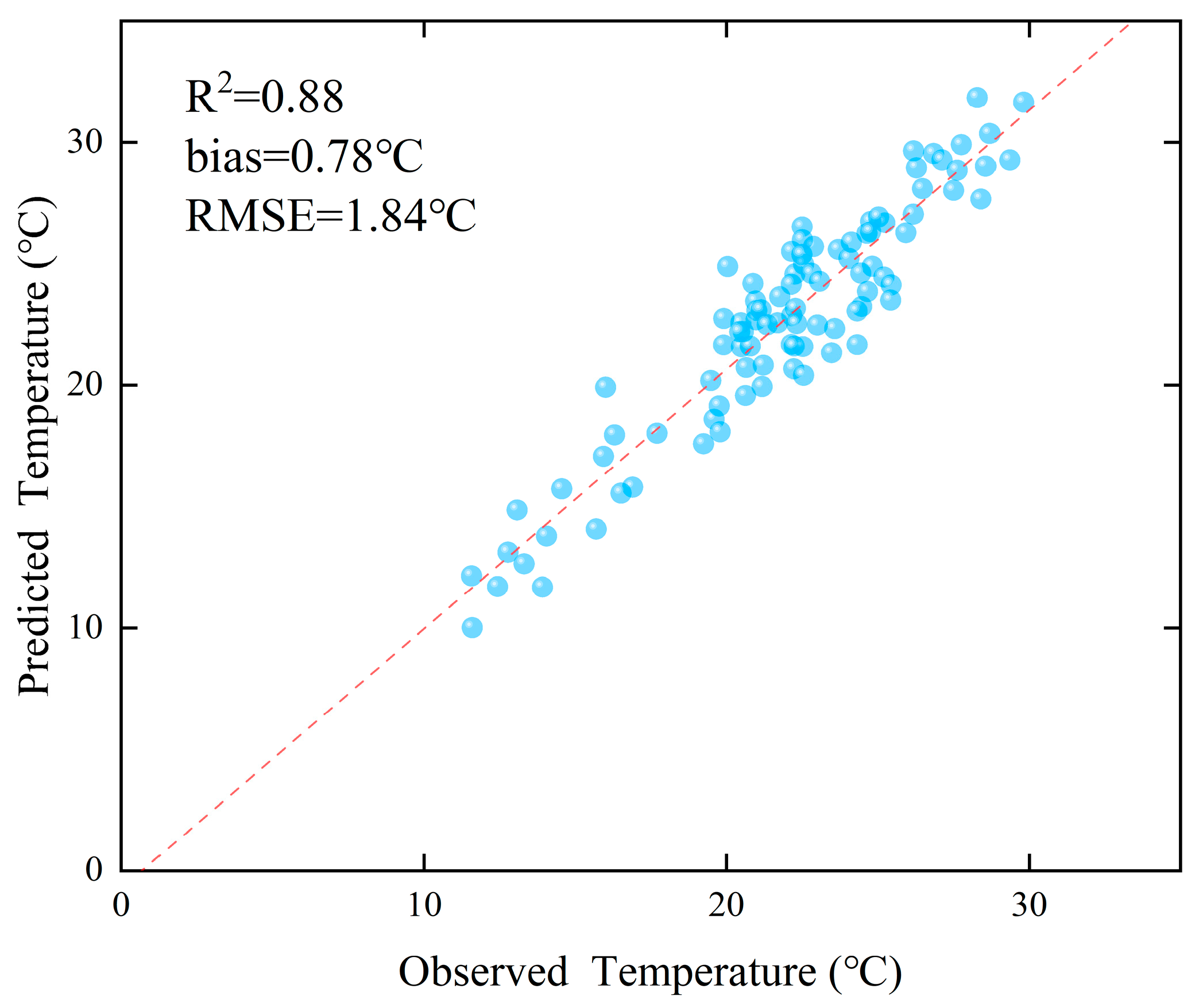
To assess the stability of the temperature prediction model, measured data from 35 meteorological stations were collected for the period June–August, 2020–2023. These observations were used to evaluate the mapping accuracy of the summer temperature spatial distribution during the same period. As shown in Figure 18, the predicted values closely match the observed temperatures (R2 = 0.88, bias = 0.78 °C, RMSE = 1.84 °C), indicating that the LSTM model can reliably predict national-scale summer temperature patterns with high accuracy.

4. Discussion

4.1. Comparison with Existing Research

Recent advances in NSAT retrieval and prediction using multi-source remote sensing data have achieved substantial progress. However, most existing technical frameworks still rely on single-region models, which are generally effective only at limited spatial scales [78]. Given China’s vast territorial extent, complex topography, and heterogeneous vegetation cover, conventional single-model approaches are inadequate for national-scale NSAT retrieval. For example, previous nationwide studies without spatial partitioning—such as Wang [79]—achieved overall accuracies with R2 values of approximately 0.84 (RMSE = 1.02 °C) and 0.87, respectively. Although Wang’s Bayesian Maximum Entropy model improved interpolation accuracy by integrating MODIS data with meteorological station observations, its performance declined in topographically complex or data-sparse areas.
In light of the pronounced heterogeneity of China’s topography–vegetation complex, this study proposes an innovative paradigm for NSAT retrieval that couples deep learning with vegetation-type partitioning. First, the dominant influencing factors in each vegetation region were identified using geographic detectors. Then, a dual-model comparison framework—comprising backpropagation neural network (BPNN) and deep neural network (DNN) models—was implemented for each region. This regionalized modeling strategy enables localized optimization, achieving R2 values of 0.94 (RMSE = 0.56 °C) in Region I and 0.96 (RMSE = 0.55 °C) in Region VII, even in areas with limited training samples. Compared with previous studies on regional-scale temperature retrieval (R2 = 0.90–0.98, RMSE = 0.87–1.46 °C), the R2 values achieved here are comparable, whereas the RMSE values show a notable improvement—by up to approximately 0.6 °C [80,81,82]. Finally, an LSTM model was integrated to perform spatial and temporal predictions of national summer temperatures on an annual basis. The results show that the LSTM model achieved R2 values in the range of 0.69–0.71, significantly outperforming previous small-area NSAT prediction studies (R2 = 0.45–0.52) [83], with improved reliability. Moreover, the combined DNN–LSTM framework demonstrated strong transferability across regions: models trained in one vegetation zone maintained high accuracy when applied to ecologically similar but spatially distinct zones, indicating their potential applicability to other large, topographically diverse countries. These findings confirm that incorporating vegetation-based partitioning is not only methodologically innovative but also essential for robust large-scale NSAT retrieval and prediction in heterogeneous environments.

4.2. Prospects for Future Research

Although this study refines the understanding of vegetation cover’s influence on SANAST by delineating distinct vegetation regions and enhancing the relevance of regional-scale analysis, certain limitations remain in its predictive capability. First, the remote sensing data used in this study have relatively low temporal resolution, limiting their ability to accurately capture short-term SANAST dynamics—particularly during extreme weather events—thereby reducing model responsiveness. In addition, this study focuses primarily on summer temperatures in China. In winter, model performance may be less stable due to the predominance of herbaceous vegetation and deciduous forests in most regions—except for subtropical evergreen broadleaf and tropical rainforest zones—where vegetation exerts a weaker regulatory influence on SANAST. Future research could enhance predictive performance by incorporating longer meteorological time series and integrating multi-source remote sensing datasets.
Furthermore, both the training and validation of seasonal predictions relied on meteorological station observations. While station data offer reliable ground-truth information, their limited number and uneven spatial distribution—especially in mountainous and sparsely populated regions—may constrain model performance by reducing accuracy and representativeness at the national scale. Future work should integrate reanalysis datasets or satellite-derived gridded products to provide more spatially continuous reference data, thereby improving model calibration, prediction accuracy, and validation robustness.

5. Conclusions

Based on China’s vegetation type zoning, this study employed a data-driven framework integrating DNN for retrieving SANAST with an LSTM model for SANAST prediction. This integrated approach enabled a comprehensive analysis of the spatiotemporal evolution of summer temperatures across China’s diverse vegetation regions.
(1)
Nighttime land surface temperature (LST_Night), elevation (DEM), and air pressure (PRS) emerged as the primary drivers of temperature variation across vegetation regions, with their influence further amplified when combined with other environmental variables. The eastern regions are influenced by both anthropogenic activities and topographic factors, whereas the western regions—particularly the Qinghai–Tibet Plateau and non-monsoon zones—are predominantly shaped by natural factors. Furthermore, in regions with substantial vegetation cover, vegetation-related factors generally contribute more than 20% to temperature variation, whereas in temperate desert areas their contribution is below 10%, indicating that vegetation plays a major role in SANAST changes in most regions.
(2)
By integrating multi-source remote sensing, geographic, and meteorological datasets, and employing region-specific modeling tailored to vegetation types, the DNN models achieved high fitting accuracy (R2 = 0.90–0.97) and low RMSE values (0.46–0.64 °C) across vegetation regions. Compared with BPNN models, the DNN approach demonstrated superior accuracy and stability, markedly improving the spatial adaptability and reliability of SANSAT retrieval at the national scale.
(3)
Building on these results, an LSTM network was applied to predict SANAST for 2020–2023. The model achieved R2 values of 0.71 and 0.69 for the training and testing sets, respectively, with corresponding RMSE values of 4.42 °C and 4.60 °C. The predicted spatial patterns were consistent with observed summer climate distributions across China, confirming the model’s feasibility and stability for time-series forecasting.
In conclusion, this study advances SANAST retrieval and prediction by overcoming the spatial constraints inherent in conventional modeling approaches. By integrating geographic detectors for environmental factor screening with multi-source remote sensing and deep learning algorithms, it develops a high-precision, scalable framework for SANAST retrieval and forecasting. This approach not only provides a novel methodological basis for exploring long-term spatiotemporal SANAST patterns under climate change but also supports regional adaptation planning. Nevertheless, the current focus on SANAST and the limited responsiveness to short-term extreme events underscore the need for future research to enhance temporal coverage and generalizability.

Author Contributions

Conceptualization, methodology, resources, W.L.; writing—original draft preparation, data curation, Z.L. (Zhefan Li); project administration, Y.W.; validation, S.X. and J.O.; supervision, J.W.; methodology, formal analysis, writing—review and editing, Z.L. (Zhenhua Liu); investigation, J.S. and M.J.; visualization, Y.L. and Z.G.; software, Z.J. and Q.F. All authors have read and agreed to the published version of the manuscript.

Funding

This research was funded by the Guangdong province science and technology plan project grant number No. 2021B1212050026.

Data Availability Statement

The data that support the findings of this study are available from the corresponding author upon reasonable request.

Acknowledgments

The authors are grateful to the editors and anonymous reviewers for their constructive comments.

Conflicts of Interest

The authors declare no conflicts of interest.

References

  1. Ma, W.; Zhou, L.; Zhang, H.; Zhang, Y.; Dai, X. Air temperature field distribution estimations over a Chinese mega-city using MODIS land surface temperature data: The case of Shanghai. Front. Earth Sci. 2016, 10, 38–48. [Google Scholar] [CrossRef]
  2. Prihodko, L.; Goward, S.N. Estimation of air temperature from remotely sensed surface observations. Remote Sens. Environ. 1997, 60, 335–346. [Google Scholar] [CrossRef]
  3. Obahoundje, S.; N’Guessan Bi, V.H.; Diedhiou, A.; Kravitz, B.; Moore, J.C. Influence of stratospheric aerosol geoengineering on temperature mean and precipitation extremes indices in Africa. Int. J. Clim. Chang. Strat. Manag. 2022, 14, 399–423. [Google Scholar] [CrossRef]
  4. Zhou, X.; Yi, Z.; Wang, Y.; Wang, D.; Zhang, L.; Huo, H. Estimating near-surface air temperature in urban functional zones in China using spatial-temporal attention. Build. Environ. 2025, 276, 112860. [Google Scholar] [CrossRef]
  5. Xue, X.; Wu, Y.-X.; Chen, Z.; Liu, R.; Zhao, Z. Interannual variation and statistical prediction of summer dry and hot days in South China from 1970 to 2018. J. Trop. Meteorol. 2023, 29, 431–447. [Google Scholar] [CrossRef]
  6. Liu, T.; Chen, H.; Jiang, W.; Li, Z. Prediction of summer precipitation in China based on soil moisture and interannual increment approach. Atmos. Sci. 2016, 40, 591–603. [Google Scholar] [CrossRef]
  7. Jiang, Y.; Fan, G.; Zhou, D.; Wu, Z. Changes in autumn persistent rain in Sichuan and its spatial distribution. Meteorol. Sci. 2013, 33, 316–324. [Google Scholar] [CrossRef]
  8. Fan, Z.; Yue, T.; Chen, C.; Sun, X. Analysis of spatial and temporal variation trends of temperature and precipitation in China. J. Earth Inf. Sci. 2011, 13, 526–533. [Google Scholar] [CrossRef]
  9. Shen, D.; Shi, W.-F.; Tang, W.; Wang, Y.; Liao, J. The agricultural economic value of weather forecasting in China. Sustainability 2022, 14, 17026. [Google Scholar] [CrossRef]
  10. Shi, Y.; Jiang, Z.; Dong, L.; Shen, S. Statistical estimation of high-resolution surface air temperature from MODIS over the Yangtze River Delta, China. J. Meteorol. Res. 2017, 31, 448–454. [Google Scholar] [CrossRef]
  11. Vancutsem, C.; Ceccato, P.; Dinku, T.; Connor, S.J. Evaluation of MODIS land surface temperature data to estimate air temperature in different ecosystems over Africa. Remote Sens. Environ. 2010, 114, 449–465. [Google Scholar] [CrossRef]
  12. Jiang, P.; Ye, S.; Chen, D.; Liu, Y.; Xia, P. Retrieving precipitable water vapor data using GPS zenith delays and global reanalysis data in China. Remote Sens. 2016, 8, 389. [Google Scholar] [CrossRef]
  13. Dirksen, M.; Knap, W.H.; Steeneveld, G.J.; Ronda, R.J. Downscaling daily air-temperature measurements in the Netherlands. Theor. Appl. Climatol. 2020, 142, 751–767. [Google Scholar] [CrossRef]
  14. Ding, X.; Zhao, Y.; Fan, Y.; Li, Y.; Ge, J. Machine learning-assisted mapping of city-scale air temperature: Using sparse meteorological data for urban climate modeling and adaptation. Build. Environ. 2023, 234, 110211. [Google Scholar] [CrossRef]
  15. Sun, Y.J.; Wang, J.F.; Zhang, R.H.; Gillies, R.R.; Xue, Y.; Bo, Y.C. Air temperature retrieval from remote sensing data based on thermodynamics. Theor. Appl. Climatol. 2005, 80, 37–48. [Google Scholar] [CrossRef]
  16. Navarro-Serrano, F.; López-Moreno, J.I.; Azorin-Molina, C.; Alonso-González, E.; Aznarez-Balta, M.; Buisán, S.T.; Revuelto, J. Elevation effects on air temperature in a topographically complex mountain valley in the Spanish Pyrenees. Atmosphere 2020, 11, 656. [Google Scholar] [CrossRef]
  17. Jiang, K.; Pan, Z.; Pan, F.; Wang, J.; Han, G.; Song, Y.; Zhang, Z.; Huang, N.; Ma, S.; Chen, X.; et al. The global spatiotemporal heterogeneity of land surface-air temperature difference and its influencing factors. Sci. Total Environ. 2022, 838, 156214. [Google Scholar] [CrossRef]
  18. Che, J.; Ding, M.; Zhang, Q.; Wang, Y.; Sun, W.; Wang, Y.; Wang, L.; Huai, B. Reconstruction of near-surface air temperature over the Greenland Ice Sheet based on MODIS data and machine learning approaches. Remote Sens. 2022, 14, 5775. [Google Scholar] [CrossRef]
  19. Sun, H.; Gao, J.; Yan, T.; Hu, K.; Xu, Z.; Wang, Y.; Meng, J.; Zhao, Z. Research progress in remote sensing monitoring of vegetation drought. J. Remote Sens. 2024, 28, 1395–1411. [Google Scholar] [CrossRef]
  20. Benali, A.; Carvalho, A.C.; Nunes, J.P.; Carvalhais, N.; Santos, A. Estimating air surface temperature in Portugal using MODIS LST data. Remote Sens. Environ. 2012, 124, 108–121. [Google Scholar] [CrossRef]
  21. Lin, X.; Zhang, W.; Huang, Y.; Sun, W.; Han, P.; Yu, L.; Sun, F. Empirical estimation of near-surface air temperature in China from MODIS LST data by considering physiographic features. Remote Sens. 2016, 8, 629. [Google Scholar] [CrossRef]
  22. Yu, L.; Jin, X. A regime-dependent retrieval algorithm for near-surface air temperature and specific humidity from multi-microwave sensors. Remote Sens. Environ. 2018, 215, 199–216. [Google Scholar] [CrossRef]
  23. Friedl, M.A.; McIver, D.K.; Hodges, J.C.F.; Zhang, X.Y.; Muchoney, D.; Strahler, A.H.; Woodcock, C.E.; Gopal, S.; Schneider, A.; Cooper, A.; et al. Global land cover mapping from MODIS: Algorithms and early results. Remote Sens. Environ. 2002, 83, 287–302. [Google Scholar] [CrossRef]
  24. Lin, S.; Moore, N.J.; Messina, J.P.; DeVisser, M.H.; Wu, J. Evaluation of estimating daily maximum and minimum air temperature with MODIS data in east Africa. Int. J. Appl. Earth Obs. Geoinf. 2012, 18, 128–140. [Google Scholar] [CrossRef]
  25. Montanaro, M.; Gerace, A.; Rohrbach, S. Toward an operational stray light correction for the Landsat 8 thermal infrared sensor. Appl. Opt. 2015, 54, 3704–3715. [Google Scholar] [CrossRef]
  26. Santana, R.A.; Dias-Júnior, C.Q.; Vale, R.D.; Tóta, J.; Fitzjarrald, D.R. Observing and modeling the vertical wind profile at multiple sites in and above the Amazon rainforest canopy. Adv. Meteorol. 2017, 2017, 1–8. [Google Scholar] [CrossRef]
  27. Eccel, E.; Ghielmi, L.; Granitto, P.; Barbiero, R.; Grazzini, F.; Cesari, D. Prediction of minimum temperatures in an Alpine region by linear and non-linear post-processing of meteorological models. Nonlinear Process. Geophys. 2007, 14, 211–222. [Google Scholar] [CrossRef]
  28. Jiang, P.; Pan, X.M.; Zeng, X.Y. Temporal and spatial variation of temperature and precipitation in each agricultural sub-region of China. Res. Soil Water Conserv. 2020, 27, 270–278. [Google Scholar] [CrossRef]
  29. Yang, D.; Zhong, S.; Mei, X.; Ye, X.; Niu, F.; Zhong, W. A comparative study of several popular models for near-land surface air temperature estimation. Remote Sens. 2023, 15, 1136. [Google Scholar] [CrossRef]
  30. Ji, Y.; Zhou, G.; Luo, T.; Dan, Y.; Zhou, L.; Lv, X. Variation of net primary productivity and its drivers in China’s forests during 2000–2018. Forest Ecosyst. 2020, 7, 15. [Google Scholar] [CrossRef]
  31. Zhang, H.; Jin, Y.; Shen, X.; Li, G.; Zhou, D. Rising air temperature and its asymmetry under different vegetation regions in China. Sci. Geogr. Sin. 2018, 38, 272–283. [Google Scholar] [CrossRef]
  32. Bonan, G. Forests and climate change: Forcings, feedbacks, and the climate benefits of forests. Science 2008, 320, 1444–1449. [Google Scholar] [CrossRef] [PubMed]
  33. Piao, S.; Yin, G.; Tan, J.; Cheng, L.; Huang, M.; Li, Y.; Liu, R.; Mao, J.; Myneni, R.B.; Peng, S.; et al. Detection and attribution of vegetation greening trend in China over the last 30 years. Global Change Biol. 2015, 21, 1601–1609. [Google Scholar] [CrossRef] [PubMed]
  34. Shen, L.; He, J.; Zhou, X.; Chen, L.; Zhu, C. The regional variabilities of the summer rainfall in China and its relation with anomalous moisture transport during the recent 50 years. Acta Meteorol. Sin. 2010, 68, 918–931. [Google Scholar] [CrossRef]
  35. Li, J.-X.; Liu, G.; Wu, R.; Ren, H.-L.; Wang, H.-M.; Mao, X.; Wei, X.-C. Narrow and wide India–Burma trough-like circulations: Their different impacts on precipitation over southern China. Geosci. Lett. 2022, 9, 7. [Google Scholar] [CrossRef]
  36. Yao, Y.; Zhang, B. MODIS-based estimation of air temperature of the Tibetan Plateau. J. Geogr. Sci. 2013, 23, 627–640. [Google Scholar] [CrossRef]
  37. Wu, G.; Zhou, X.; Xu, X.; Huang, J.; Duan, A.; Yang, S.; Hu, W.; Ma, Y.; Liu, Y.; Bian, J.; et al. An integrated research plan for the Tibetan Plateau land–air coupled system and its impacts on the global climate. Bull. Am. Meteorol. Soc. 2023, 104, E158–E177. [Google Scholar] [CrossRef]
  38. Jang, K.; Kang, S.; Kimball, J.S.; Hong, S.Y. Retrievals of all-weather daily air temperature using MODIS and AMSR-E data. Remote Sens. 2014, 6, 8387–8404. [Google Scholar] [CrossRef]
  39. Ding, L.; Zhou, J.; Zhang, X.; Wang, S.; Tang, W.; Wang, Z.; Ma, J.; Ai, L.; Li, M.; Wang, W. Progress and challenges in all-weather remote sensing of land surface temperature. J. Remote Sens. 2023, 27, 1534–1553. [Google Scholar] [CrossRef]
  40. Sheffield, J.; Wood, E.F.; Pan, M.; Beck, H.; Coccia, G.; Serrat-Capdevila, A.; Verbist, K. Satellite remote sensing for water resources management: Potential for supporting sustainable development in data-poor regions. Water Resour. Res. 2018, 54, 9724–9758. [Google Scholar] [CrossRef]
  41. Foga, S.; Scaramuzza, P.L.; Guo, S.; Zhu, Z.; Dilley, R.D.; Beckmann, T.; Schmidt, G.L.; Dwyer, J.L.; Hughes, M.J.; Laue, B. Cloud detection algorithm comparison and validation for operational Landsat data products. Remote Sens. Environ. 2017, 194, 379–390. [Google Scholar] [CrossRef]
  42. Zhu, Z.; Wang, S.; Woodcock, C.E. Improvement and expansion of the Fmask algorithm: Cloud, cloud shadow, and snow detection for Landsats 4, 7, 8, and Sentinel 2 images. Remote Sens. Environ. 2015, 159, 269–277. [Google Scholar] [CrossRef]
  43. Qiu, Y.; Chai, D. A deep learning method for Landsat image cloud detection without manually labeled data. Remote Sens. Land Resour. 2021, 33, 102–107. [Google Scholar] [CrossRef]
  44. Yang, X.; Tang, G.; Xiao, C.; Deng, F. Terrain revised model for air temperature in mountainous area based on DEMs: A case study in Yaoxian county. J. Geogr. Sci. 2007, 17, 399–408. [Google Scholar] [CrossRef]
  45. Zhu, S.; Zhou, C.; Zhang, G.; Zhang, H.; Hua, G. Preliminary verification of instantaneous air temperature estimation for clear sky conditions based on SEBAL. Meteorol. Atmos. Phys. 2017, 129, 71–81. [Google Scholar] [CrossRef]
  46. Tucker, C.J. Red and Photographic Infrared Linear Combinations for Monitoring Vegetation. Remote Sens. Environ. 1979, 8, 127–150. [Google Scholar] [CrossRef]
  47. Janatian, N.; Sadeghi, M.; Sanaeinejad, S.H.; Bakhshian, E.; Farid, A.; Hasheminia, S.M.; Ghazanfari, S. A statistical framework for estimating air temperature using MODIS land surface temperature data. Int. J. Climatol. 2017, 37, 1181–1194. [Google Scholar] [CrossRef]
  48. Zhang, X.; Jiao, Z.; Zhao, C.; Qu, Y.; Liu, Q.; Zhang, H.; Tong, Y.; Wang, C.; Li, S.; Guo, J.; et al. Review of land surface albedo: Variance characteristics, climate effect and management strategy. Remote Sens. 2022, 14, 1382. [Google Scholar] [CrossRef]
  49. Liang, S.; Wang, K.; Zhang, X.; Wild, M. Review on estimation of land surface radiation and energy budgets from ground measurement, remote sensing and model simulations. IEEE J. Sel. Top. Appl. Earth Obs. Remote Sens. 2010, 3, 225–240. [Google Scholar] [CrossRef]
  50. Chen, A.; Meng, W.; Hu, S.; Bian, L. Comparative analysis on land surface albedo from MODIS and GLASS over the Tibetan Plateau. Trans. Atmos. Sci. 2020, 43, 932–942. [Google Scholar] [CrossRef]
  51. Wang, L.; Zheng, X.; Sun, L.; Liu, Q.; Liu, S. Validation of GLASS albedo product through Landsat TM data and ground measurements. J. Remote Sens. 2014, 18, 547–558. [Google Scholar] [CrossRef]
  52. Andres-Anaya, P.; Sanchez-Aparicio, M.; Del Pozo, S.; Lagüela, S.; Hernández-López, D.; Gonzalez-Aguilera, D. A new methodology for estimating surface albedo in heterogeneous areas from satellite imagery. Appl. Sci. 2024, 14, 75. [Google Scholar] [CrossRef]
  53. Julien, Y.; Sobrino, J.A.; Jiménez-Muñoz, J.-C. Land use classification from multitemporal Landsat imagery using the Yearly Land Cover Dynamics (YLCD) method. Int. J. Appl. Earth Obs. Geoinf. 2011, 13, 711–720. [Google Scholar] [CrossRef]
  54. Karmaoui, A.; Moumane, A.; El Jaafari, S.; Menouni, A.; Al Karkouri, J.; Yacoubi, M.; Hajji, L. Thirty years of change in the land use and land cover of the Ziz Oases (Pre-Sahara of Morocco) combining remote sensing, GIS, and field observations. Land 2023, 12, 2127. [Google Scholar] [CrossRef]
  55. Li, Z.; Zhou, Z.; Liu, Z.; Si, J.; Ou, J. Assessment and dynamic prediction of green space ecological service value in Guangzhou City, China. Remote Sens. 2024, 16, 4180. [Google Scholar] [CrossRef]
  56. Camps-Valls, G.; Campos-Taberner, M.; Moreno-Martínez, Á.; Walther, S.; Duveiller, G.; Cescatti, A.; Mahecha, M.D.; Muñoz-Marí, J.; García-Haro, F.J.; Guanter, L.; et al. A unified vegetation index for quantifying the terrestrial biosphere. Sci. Adv. 2021, 7, eabc7447. [Google Scholar] [CrossRef]
  57. Wang, C.; Liu, L.; Zhou, Y.; Liu, X.; Wu, J.; Tan, W.; Xu, C.; Xiong, X. Comparison between satellite derived solar-induced chlorophyll fluorescence, NDVI and kNDVI in detecting water stress for dense vegetation across southern China. Remote Sens. 2024, 16, 1735. [Google Scholar] [CrossRef]
  58. Lu, J.; Li, J.; Fu, H.; Tang, X.; Liu, Z.; Chen, H.; Sun, Y.; Ning, X. Deep learning for multi-source data-driven crop yield prediction in Northeast China. Agriculture 2024, 14, 794. [Google Scholar] [CrossRef]
  59. Jordan, C.F. Derivation of leaf-area index from quality of light on the forest floor. Ecology 1969, 50, 663–666. [Google Scholar] [CrossRef]
  60. Bao, N.; Li, W.; Gu, X.; Liu, Y. Biomass estimation for semiarid vegetation and mine rehabilitation using Worldview-3 and Sentinel-1 SAR imagery. Remote Sens. 2019, 11, 2855. [Google Scholar] [CrossRef]
  61. Vijith, H.; Dodge-Wan, D. Applicability of MODIS land cover and Enhanced Vegetation Index (EVI) for the assessment of spatial and temporal changes in strength of vegetation in tropical rainforest region of Borneo. Remote Sens. Appl. Soc. Environ. 2020, 18, 100311. [Google Scholar] [CrossRef]
  62. Hao, B.; Xu, X.; Wu, F.; Tan, L. Long-term effects of fire severity and climatic factors on post-forest-fire vegetation recovery. Forests 2022, 13, 883. [Google Scholar] [CrossRef]
  63. Liu, J.; Xu, Y.; Li, H.; Guo, J. Soil moisture retrieval in farmland areas with Sentinel multi-source data based on regression convolutional neural networks. Sensors 2021, 21, 877. [Google Scholar] [CrossRef]
  64. Wu, Z.; Zhang, X.; Ma, P.; Kwan, M.-P.; Liu, Y. How did urban environmental characteristics influence land surface temperature in Hong Kong from 2017 to 2022? Evidence from remote sensing and land use data. Sustainability 2023, 15, 15511. [Google Scholar] [CrossRef]
  65. Wang, J.; Zhang, T.; Fu, B. A measure of spatial stratified heterogeneity. Ecol. Indic. 2016, 67, 250–256. [Google Scholar] [CrossRef]
  66. Chen, Q.; Zhang, L.; Duan, Y.; Fan, S. Spatial and temporal patterns and evolution of traditional villages in Jiangxi Province. J. Remote Sens. 2021, 25, 2460–2471. [Google Scholar] [CrossRef]
  67. Zhang, X.; Lyu, C.; Fan, X.; Bi, R.; Xia, L.; Xu, C.; Sun, B.; Li, T.; Jiang, C. Spatiotemporal variation and influence factors of habitat quality in Loess Hilly and Gully Area of Yellow River Basin: A case study of Liulin County, China. Land 2022, 11, 127. [Google Scholar] [CrossRef]
  68. Zhao, Y.; Luo, L.; Wan, H.; Wu, Q.; Liu, C. Remote sensing monitoring and analysis of landscape pattern changes in Bayinbuluke Heritage Area over the past 30 years. J. Remote Sens. 2021, 25, 2488–2506. [Google Scholar] [CrossRef]
  69. Li, J.; Huang, X.; Gong, J. Deep neural network for remote-sensing image interpretation: Status and perspectives. Natl. Sci. Rev. 2019, 6, 1082–1086. [Google Scholar] [CrossRef] [PubMed]
  70. Rumelhart, D.E.; Hinton, G.E.; Williams, R.J. Learning representations by back-propagating errors. Nature 1986, 323, 533–536. [Google Scholar] [CrossRef]
  71. Tian, S.; Ma, L.; Li, H.; Tian, F.; Mao, J. Research on a coal seam gas content prediction method based on an improved extreme learning machine. Appl. Sci. 2023, 13, 8753. [Google Scholar] [CrossRef]
  72. He, X.; Zhao, X.; Sun, Y.; Geng, P.; Zhang, X. Application of TBSS-based machine learning models in the diagnosis of pediatric autism. Front. Neurol. 2023, 13, 1078147. [Google Scholar] [CrossRef]
  73. El Ghaoui, L.; Gu, F.; Travacca, B.; Askari, A.; Tsai, A. Implicit deep learning. SIAM J. Math. Data Sci. 2021, 3, 930–958. [Google Scholar] [CrossRef]
  74. Hochreiter, S.; Schmidhuber, J. Long short-term memory. Neural Comput. 1997, 9, 1735–1780. [Google Scholar] [CrossRef]
  75. Mehrkanoon, S. Deep shared representation learning for weather elements forecasting. Knowl.-Based Syst. 2019, 179, 120–128. [Google Scholar] [CrossRef]
  76. Hutasavi, S.; Chen, D. Estimating district-level electricity consumption using remotely sensed data in Eastern Economic Corridor, Thailand. Remote Sens. 2021, 13, 4654. [Google Scholar] [CrossRef]
  77. Zhu, J.; Cao, S.; Shang, G.; Shi, J.; Wang, X.; Zheng, Z.; Liu, C.; Yang, H.; Xie, B. Subpixel snow mapping using daily AVHRR/2 data over Qinghai–Tibet Plateau. Remote Sens. 2022, 14, 2899. [Google Scholar] [CrossRef]
  78. Jiang, Y.; Li, T.; Cheng, Q.; Shen, H.-F. Inversion of air temperature in the Yangtze River Economic Belt using spatiotemporal neural network model. J. Trop. Meteorol. 2023, 48, 325–332. [Google Scholar] [CrossRef]
  79. Wang, M. Spatial Estimation of Air Temperature Based on Multi-Source Information Fusion and Its Application. Master’s Thesis, Hubei University, Wuhan, China, 2021. [Google Scholar]
  80. Jang, J.D.; Viau, A.A.; Anctil, F. Neural network estimation of air temperatures from AVHRR data. Int. J. Remote Sens. 2004, 25, 4541–4554. [Google Scholar] [CrossRef]
  81. Bai, J.; Zhang, Y. Regression model of spatial air-temperature distribution and monthly variation characteristics in Sichuan Province. Sichuan Meteorol. 2006, 2, 17–18. [Google Scholar]
  82. Bai, L.; Xu, Y.M.; He, M.; Li, N. Study on remote sensing retrieval of near-surface air temperature based on random forest algorithm. J. Geo-Inf. Sci. 2017, 19, 390–397. [Google Scholar]
  83. Han, P.; Ji, Z. Ridge regression prediction model for May air temperature in South China. J. Appl. Meteorol. Sci. 2024, 35, 480–492. [Google Scholar] [CrossRef]
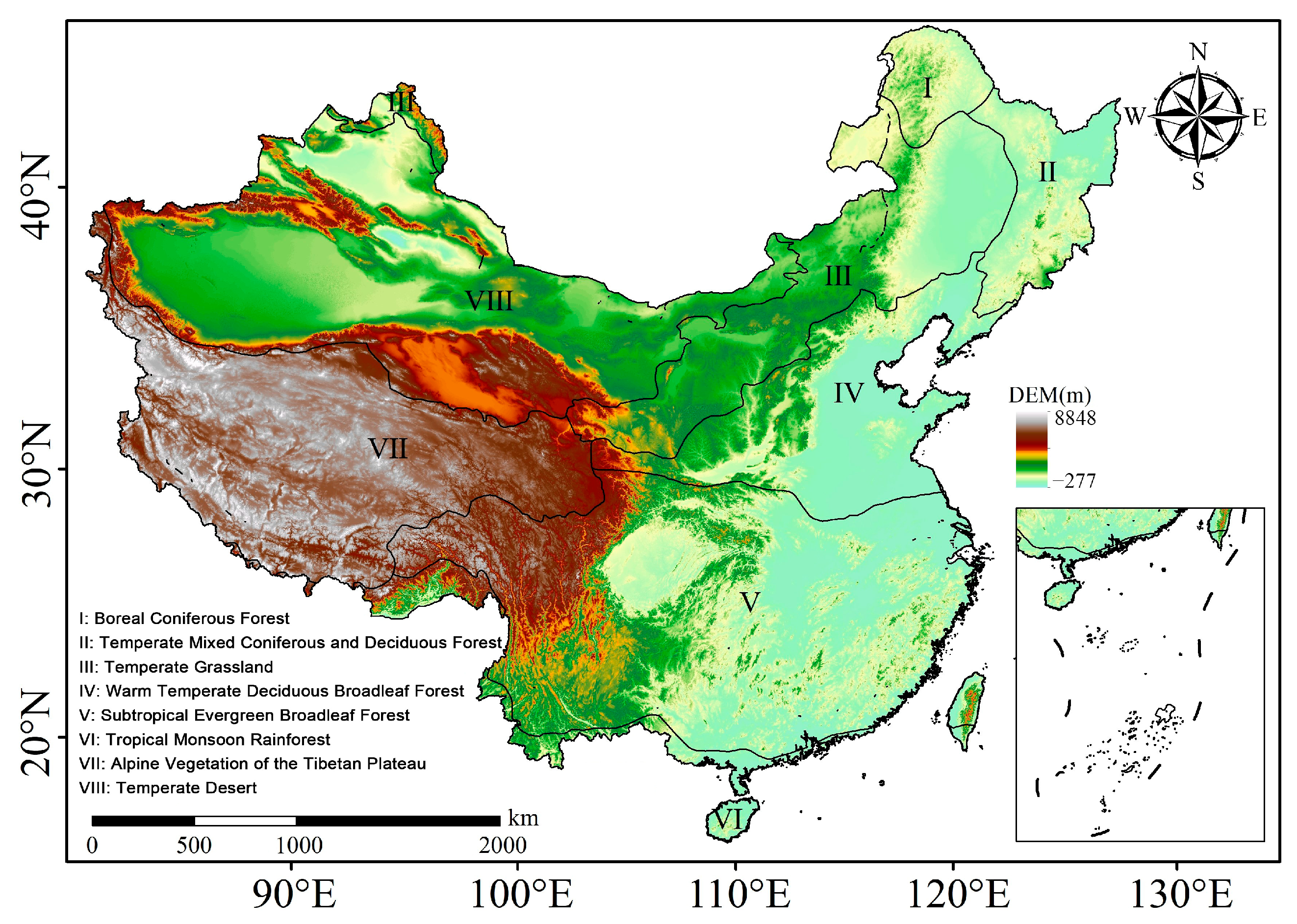
Figure 1. The study area.
Remotesensing 17 03209 g001
Figure 2. Distribution map of meteorological stations.
Remotesensing 17 03209 g002
Figure 3. Overall research framework.
Remotesensing 17 03209 g003
Figure 4. Overall research framework.
Remotesensing 17 03209 g004
Figure 5. Typical BP neural network structure.
Remotesensing 17 03209 g005
Figure 6. Structure diagram of the LSTM algorithm.
Remotesensing 17 03209 g006
Figure 7. Spatial distribution of variables in the study area: (a) daytime land surface temperature (LST_Day); (b) nighttime land surface temperature (LST_Night); (c) solar radiation (SA); (d) digital elevation model (DEM); (e) soil moisture (SM); (f) relative humidity (RH); (g) sunshine hours (SH); (h) wind speed (WS); (i) surface pressure (PRS); (j) population density (PD); (k) normalized difference vegetation index (NDVI); (l) kernel normalized difference vegetation index (KNDVI); (m) difference vegetation index (DVI); (n) enhanced vegetation index (EVI); (o) modified soil-adjusted vegetation index (MSAVI).
Remotesensing 17 03209 g007
Figure 8. The results of factor detector in each vegetation region: (I) Cold temperate coniferous forest region; (II) Temperate coniferous and deciduous mixed forest region; (III) Temperate grassland region; (IV) Warm temperate deciduous broad-leaved forest region; (V) Subtropical evergreen broad-leaved forest region; (VI) Tropical monsoon forest and rainforest region; (VII) Alpine vegetation region in the Qinghai–Tibet Plateau; (VIII) Temperate desert region.
Remotesensing 17 03209 g008
Figure 9. Interaction detection results of various vegetation regions. Note: ** indicates two-factor enhancement, * indicates nonlinear enhancement.
Remotesensing 17 03209 g009
Figure 10. (ah) Scatter plot of comparison between observed value and retrieved value of training set based on DNN model; (ip) scatter chart of comparison between observed value and retrieved value of training set based on BPNN model.
Remotesensing 17 03209 g010
Figure 11. (ah) Scatter plot of comparison between observed value and retrieved value of test set based on DNN model; (ip) scatter chart of comparison between observed value and retrieved value of test set based on BPNN model.
Remotesensing 17 03209 g011
Figure 12. Spatial distribution map of summer average SANAST from 2000 to 2019. Panels (at) correspond to individual years from 2000 to 2019.
Remotesensing 17 03209 g012
Figure 13. Scatter chart of SANAST observed value and retrieved value in graphical verification set.
Remotesensing 17 03209 g013
Figure 14. Spatial distribution of summer average near-surface air temperature (SANAST, °C) in 2018 derived from different methods: (a) SANAST distribution based on the DNN model; (b) SANAST distribution based on Kriging interpolation, with four representative subregions (1–4) marked by red rectangles; (c) Zoom-in comparisons of the four subregions (columns 1–4 correspond to the regions marked in panel (b)): top row — DNN results; bottom row—Kriging interpolation results.
Remotesensing 17 03209 g014
Figure 15. R2 curve of SANAST prediction model under different time steps.
Remotesensing 17 03209 g015
Figure 16. Scatter chart of comparison between observed value and estimated value of the SANAST prediction model. Note: part (a) shows the training set and part (b) shows the test set.
Remotesensing 17 03209 g016
Figure 17. Spatial distribution map of SANAST (unit: ℃) in China from 2020 to 2023: (a) 2020; (b) 2021; (c) 2022; (d) 2023.
Remotesensing 17 03209 g017
Figure 18. Comparison scatter chart between measured and predicted temperature values.
Remotesensing 17 03209 g018
Table 1. Source and attribute of satellite data.
Data TypeDataset SourceTime ResolutionSpatial Resolution
Surface temperatureMODIS Land surface temperature and emissivity dataset (MOD11A1)Daily1 km
Vegetation indexMODIS Vegetation index dataset (MOD13A2)8 days1 km
Surface albedoMODIS Albedo dataset (MCD43A3)9 days500 m
ElevationNASA SRTM Digital elevation dataset30 m
Soil moistureGLDAS-2.1: Global land assimilation system datasetMonthly1 km
Table 2. Quantitative distribution of sample points in each vegetation region.
Sample TypeNumber of Samples in Each Vegetation Region
IIIIIIIVVVIVIIVIII
Training set80500120017803860260360660
Test set401203805601340100120220
Verification set20100300440136080120180
Table 3. Interaction relationship.
Relationship DescriptionInteractionImplication
q X 1 X 2 < min q X 1 ,   q X 2 Nonlinear attenuationStrong negative interaction
min q X 1 ,   q X 2 < q X 1 X 2 < max q X 1 ,   q X 2 Single-factor nonlinear attenuationWeak negative interaction
q X 1 X 2 > max q X 1 ,   q X 2 Two-factor enhancementSynergistic effect
q X 1 X 2 = q X 1 + q X 2 Independent roleNo interference with each other
q X 1 X 2 >   q X 1 + q X 2 Nonlinear enhancementStrong synergistic effect
Table 4. Optimal SANAST retrieval indicators of each vegetation region.
Region CodeVegetation RegionIndicator
ICold temperate coniferous forest regionDEM, PRS, LST_Night, KNDVI, EVI, RH, LST_Day, PD, NDVI, SH, SA, SM, WS
IITemperate coniferous and deciduous forest mixed forest regionLST_Night, DEM, PRS, KNDVI, LST_Day, PD, MSAVI, SA, DVI
IIITemperate grassland regionLST_Night, DEM, PRS, LST_Day, RH, SA, NDVI, KNDVI, WS
IVWarm temperate deciduous broad-leaved forest regionLST_Night, DEM, PRS, LST_Day, WS, PD, KNDVI
VSubtropical evergreen broad-leaved forest regionLST_Night, PRS, DEM, LST_Day, PD, KNDVI, SM
VITropical monsoon forest and rainforest regionDEM, PRS, LST_Night, WS, SH, LST_Day, KNDVI, NDVI, PD, EVI, DVI, SM, MSAVI, SA
VIIAlpine vegetation region in Qinghai–Tibet PlateauLST_Night, DEM, PRS, LST_Day, RH, WS, SA, DVI, KNDVI, MSAVI, PD, EVI
VIIITemperate desert regionLST_Night, DEM, PRS, LST_Day, SH, SA, WS
Disclaimer/Publisher’s Note: The statements, opinions and data contained in all publications are solely those of the individual author(s) and contributor(s) and not of MDPI and/or the editor(s). MDPI and/or the editor(s) disclaim responsibility for any injury to people or property resulting from any ideas, methods, instructions or products referred to in the content.