Highlights
What are the main findings?
- Benchmark of four hybrid CNN-RNNs (1D/2D × LSTM/GRU) on Sentinel-2; 2D CNN-GRU leads (OA 99.12%, macro-F1 99.14%).
- Combining spatial context (2D CNN) with temporal phenology (RNN) outperforms 1D and stand-alone models.
What is the implication of the main finding?
- Hybrid spatiotemporal modeling with NDVI/red-edge indices enables accurate, operational crop mapping.
- Reporting accuracy and efficiency supports practical deployment and reproducibility.
Abstract
Accurate crop classification using satellite imagery is critical for agricultural monitoring, yield estimation, and land-use planning. However, this task remains challenging due to the spectral similarity among crops. Although crops differ in physiological characteristics, including chlorophyll content, they often exhibit only subtle differences in their spectral reflectance, which make their precise discrimination challenging. To address this, this study uses the high temporal and spectral resolution of Sentinel-2 imagery, including its red-edge bands and derived vegetation indices, which are particularly sensitive to vegetation health and structural differences. This study presents a hybrid deep learning framework for crop classification, conducted through a case study in a complex agricultural region of Northern Italy. We investigated the combined use of spectral bands and NDVI & red-edge-based vegetation indices as inputs to hybrid deep learning models. Previous studies have applied 1D CNN, 2D CNN, LSTM, and GRU, often standalone, but their capacity to jointly process spectral and vegetative features through integrated CNN-RNN structures remains underexplored in mixed agricultural regions. To fill this gap, we developed and assessed four hybrid architectures: (1) 1D CNN-LSTM, (2) 1D CNN-GRU, (3) 2D CNN-LSTM, and (4) 2D CNN-GRU. These models were trained using optimized hyperparameters on combined spectral and vegetative input features. The 2D CNN-GRU model achieved the highest overall accuracy (99.12%) and F1-macro (99.14%), followed by 2D CNN-LSTM (98.51%), while 1D CNN-GRU and 1D CNN-LSTM performed slightly lower (93.46% and 92.54%), respectively.
1. Introduction
Agriculture is a broad term encompassing a wide range of activities that refer to the production of food through cultivation, domestication, vegeculture, arboriculture, and horticulture, as well as mixed crop-livestock farming [1]. During the 20th century, crop production in the Green Revolution period increased due to scientific advancements. This intensification of agriculture led to greater land use, which came at the cost of resource depletion. Therefore, sustainable intensification of arable land is required to implement efficient agricultural policies [2]. In 1974, the FAO began reporting on the scale of world hunger, highlighting a critical global issue. The growing worldwide population has exacerbated malnutrition, presenting a troubling trend [3]. Despite technological advancements, global hunger rose sharply between 2019 and 2021 and has remained at similar levels through 2023 [4]. Our current consumption patterns are unsustainable, presenting significant challenges such as hunger, inequality, and climate change, which demand urgent action to address these interconnected issues [5,6]. The Sustainable Development Goals (SDGs), particularly Goal 2, emphasize the importance of eradicating world hunger, ensuring food security, meeting nutritional needs, and promoting sustainable agriculture [7].
Efficient crop mapping with high spatial and temporal resolution can inform effective resource allocation and support food security by providing timely data on crop distribution and conditions [8,9]. Earth Observation (EO) refers to the acquisition of information about the physical, chemical, and biological properties of the Earth using satellites, airborne, and in situ sensors [10,11]. This remotely sensed data offers cost-effective and reliable measurements on a global scale, significantly reducing the reliance on ground surveys and traditional data collection methods [12,13]. Achieving the United Nations Sustainable Development Goal of “Zero Hunger” requires innovative strategies for monitoring and managing agricultural systems [14]. In this context, EO data has emerged as a vital resource in precision agriculture [15], offering timely, large-scale, and detailed insights into crop health, yield, and land use [16,17].
European Space Agency’s Copernicus program, Sentinel-2, is an EO mission that is changing the way we monitor the world’s farmlands [18]. Designed to capture high-resolution images regularly, it provides a clear and consistent view of crops over time. This makes it an incredibly useful tool for farmers, researchers, and policymakers [19]. By tracking changes in fields throughout the sowing, growing, and harvesting seasons [20]. With its ability to deliver insights on a global scale, it is becoming a key player in promoting smarter, more sustainable agriculture practices [21]. Sentinel-2 supports agricultural monitoring by providing free access to detailed high-resolution imagery with a 10 m spatial resolution, a revisit time of just 5 days, and a wide range of spectral bands, including red-edge bands critical for assessing vegetation health and crop conditions [22,23].
The use of machine learning (ML) and deep learning (DL) techniques in crop classification using satellite data has become increasingly significant in agricultural management and food security [24,25]. These technologies enable accurate mapping and monitoring of crop types over large areas. Several studies have explored the application of ML and DL models for crop classification using satellite data. Common ML models include Support Vector Machines (SVM), Random Forest (RF), K-Nearest Neighbors (KNN), and Decision Trees (DT), which have been used to classify various crop types with high accuracy [26,27,28]. DL models, particularly Convolutional Neural Networks (CNN) and Long Short-Term Memory Networks (LSTM), and Gated recurrent units (GRU) have shown superior performance in handling the complex patterns in satellite imagery, achieving high classification accuracy for different crop types [29,30,31,32].
The integration of the time series of Sentinel-2 spectral data and vegetational indices has been crucial in improving crop classification accuracy [33]. These data sources, particularly red edge, shortwave infrared, and vegetational indices, provide diverse spectral information that enhances the ability to distinguish between different crop types [34,35]. The red-edge band is pivotal in capturing subtle spectral variations associated with crop types, making it vital for effective crop discrimination [36]. By providing detailed information on green vegetation growth, this band serves for the development and application of various red-edge-based vegetation indices, which are critical for monitoring agricultural farmlands [37].
One of the main challenges in crop classification is the high intra- and inter-class variability of crops, which can lead to misclassification. Deep learning algorithms have advantages over machine learning algorithms as they can capture the spatial and temporal context of data in large-scale heterogeneous agricultural areas [38,39,40]. DL models can automatically extract and learn complex features from satellite data, reducing the need for manual feature engineering [28,41,42]. Several studies [43,44,45] have demonstrated that deep learning, when applied to satellite time-series data, achieves comparable or superior accuracy to machine learning by effectively identifying dense temporal patterns through its high computational capabilities. Reference [46] suggested that deep learning algorithms are highly efficient in distinguishing mixed or underrepresented classes.
A convolutional neural network (CNN) stands out as one of the most effective architectures in deep learning [42]. Its learning process is both computationally efficient and robust to data shifts, such as image translations, making it a top choice for identifying patterns in satellite imagery [47]. This capability makes CNN particularly well-suited for crop classification, where they excel at identifying intricate patterns and differentiating between various crops [48]. CNNs are widely used in both one-dimensional (1D) and two-dimensional (2D) forms. One-dimensional CNNs are designed to extract spectral features. In contrast, 2D CNN focus on capturing spatial features, effectively identifying patterns, textures, and shapes within two-dimensional data (width × height of the image) [49,50].
Recurrent neural networks (RNN) represent an advanced category of artificial neural networks (ANNs) distinguished by their ability to process sequential data through looped connections [51,52]. These networks are particularly adept at analyzing temporal dependencies and have demonstrated significant success in remote sensing applications. By effectively modeling sequential relationships, RNNs enable the extraction of features from multi-temporal data [48]. This is particularly important in crop classification as it helps capture crop phenological stages in plant growth. Among the variants of RNNs, long short-term memory (LSTM) networks are the most widely used due to their ability to manage long-term dependencies through gated mechanisms, addressing issues like vanishing or exploding gradients [53]. Similarly, gated recurrent units (GRU) provide an efficient alternative with simplified architecture and comparable capabilities [54]. Studies [42,48,55,56,57,58] have successfully utilized LSTM and GRU models, along with 1D and 2D convolutional neural networks (CNN). Ref. [59] reported that the greatest performance was achieved by combining both recurrent and convolutional layers. These approaches have demonstrated high accuracy in extracting spatial, spectral, and temporal features for land cover and crop type classification tasks.
The objective of this study is to demonstrate the synergy between CNNs and RNNs in handling multi-temporal remote sensing data for large-scale crop classification, which represents a novel and challenging approach. In this study, we used 1D CNN to capture spectral and temporal patterns from multi-temporal Sentinel-2 reflectance data and red-edge vegetation indices. Simultaneously, a 2D CNN extracts spatial features, such as field boundaries and textural information. The features extracted by both CNNs are then passed to LSTM or GRU separately. These RNNs are effective at modeling long-term temporal dependencies and crucial for capturing crop phenological cycles. The combined spectral, spatial, and temporal features learned through this architecture are ultimately used for accurate crop type classification.
In particular, the specific goal of this study is as follows:
- Testing the use of advanced deep learning methods on large-scale Sentinel-2 datasets, addressing the challenges of scalability and data complexity.
- Evaluating the potential of combining CNN and RNNs to handle the complexity of multi-temporal remote sensing data for crop classification.
- Assess the impact of temporal richness and spectral diversity of Sentinel-2 imagery, including red-edge indices, to improve classification accuracy.
- Develop a workflow where 1D CNN extract spectral and temporal features, 2D CNN capture spatial patterns, and RNNs (LSTM/GRU) model temporal dependencies.
- Evaluate the performance of combined 1D and 2D CNN-LSTM and CNN-GRU models against each other for crop type classification.
2. Materials and Methods
2.1. Study Area
The climatic conditions prevailing in the Italian landscape make it suitable for diverse agricultural practices over the different parts of the country. The study area covers approximately 22,446 km2, and is in northern Italy, mainly in the Emilia-Romagna region and extending into parts of Lombardy and Veneto regions, important agricultural zones (Figure 1). This territory has a temperate climate that is favorable to cultivating a variety of crops such as wheat, maize, sugar beet, and vineyards, which are pivotal for local consumption as well as export [60]. It has hot, humid summers and cold, foggy winters, with summer temperatures averaging between 25 and 30 °C and winter temperatures between 0 and 5 °C, with occasional snowfall. Mean annual rainfall ranges from 600 to 1000 mm, mostly falling in autumn and spring, supporting both rain-fed as well as irrigated agriculture.
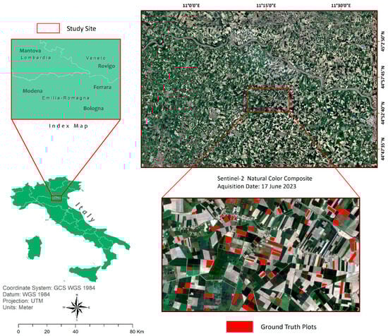
Figure 1.
Geographic location of the study site showing Sentinel-2 natural color composite image.
Agricultural activities follow a structured seasonal calendar, differentiating winter and summer crops [61]. Winter crops, such as wheat and rapeseed, are typically sown in October and November. Wheat grows from February to April and is harvested between May and June, while rapeseed matures from October to mid-June, with harvesting occurring in late June through July. Summer crops, including maize and soybeans, are planted from early to mid-spring. Maize reaches its peak growth by late July and is harvested from late August to September, while soybeans are collected from late September to mid-October. Forage crops for crop-livestock systems are sown in March or early April, with multiple harvests occurring from May to August. Sorghum and sunflowers, planted in spring, are harvested in autumn; sugar beet, sown between February and May, follows a flexible growth schedule with staggered harvesting periods. The precise scheduling of crop cycles facilitates effective crop rotation and enhances agricultural management within the region (Figure 2).
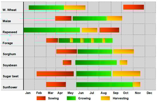
Figure 2.
Crop calendar showing the phenology of different crops present in the study area.
2.2. Data Resources
2.2.1. Satellite Data Acquisition
The Sentinel-2 mission, part of the European Earth observation program, is equipped with the Multispectral Instrument (MSI), which captures vital data across 13 spectral bands, spanning visible light, near-infrared, and shortwave infrared wavelengths [62]. Operating as a constellation with two satellites, Sentinel-2A and Sentinel-2B, the mission delivers critical information for agricultural monitoring, achieving a revisit interval of approximately five days [63,64].
Bottom-of-Atmosphere (BOA) Level 2A products, including data for tile ID T32TPQ, were accessed via the Copernicus program’s recently launched “European’s Eyes on Earth” platform https://browser.dataspace.copernicus.eu (accessed 14 December 2024). The study utilized multitemporal data corresponding to key crop growth stages, sowing, growing, and harvesting spanning the period from November 2022 to August 2023. Only imagery with less than 5% cloud coverage over the study area was included in the analysis (Figure 3). For spectral feature preparation, the 10 most relevant bands from each date were selected to ensure robust representation of crop dynamics. Figure 4 illustrates the spatial resolution and wavelengths of Sentinel-2 bands used in this study.
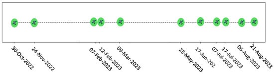
Figure 3.
Sentinel-2 multi-temporal data acquisition dates.
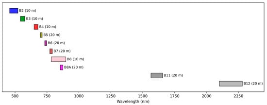
Figure 4.
Sentinel-2 bands used for feature preparation.
2.2.2. Ground Truth Data for Training, Validation, and Testing
Ground truth data for the winter crop season were collected by digitizing crop polygons using the OneSoil web portal https://map.onesoil.ai (accessed 25 June 2024)). These Polygons were validated through overlay analysis with multi-temporal Sentinel-2 data that captures different phenological crop stages. In addition, each crop’s spectral signature was cross-checked and verified against Sentinel-2 images. This process resulted in a dataset comprising 2171 polygons that represent various regional crops shown in Table 1 and Figure 1. Deep learning classifiers require balanced training datasets to achieve optimal performance [65]. However, imbalanced datasets, such as those with disproportionate representation where certain classes have fewer samples than others, can lead to overfitting issues [66]. To address this challenge, random sampling techniques were applied to balance the distribution of sampling polygons across crop classes. This ensured that the number of polygons in each crop class was proportional to its actual prevalence in the dataset. During the model training, validation, and testing process, stratified random sampling was employed. Specifically, 60% of the sampling polygons were allocated for training the classifiers, 20% were used for validation, and the remaining 20% were reserved for testing the accuracy of the results.

Table 1.
Distribution of ground truth polygons for each crop type.
2.3. Methodological Overview
The workflow of this study carried several steps, including satellite image preprocessing, time-series feature extraction, deep learning model development, classification, and result evaluation (Figure 5). Based on the prepared features, which include spectral bands and vegetation indices, four distinct deep learning models were designed: (i) 1D CNN-LSTM, (ii) 1D CNN-GRU, (iii) 2D CNN-LSTM, and (iv) 2D CNN-GRU. These models were developed to effectively use the spatial and temporal characteristics of the data for improved crop classification.
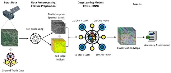
Figure 5.
Methodological workflow for this study.
2.4. Data Preprocessing
The Sentinel-2 time-series data were processed using an automated pipeline built with ESA’s SNAP GPT workflow. A custom processing graph was designed to handle each input file, ensuring all selected Sentinel-2 bands were resampled to a 10 m resolution and clipped to the boundaries of the study area. To simplify this workflow, we developed a shell script that automated the execution of all SNAP GPT commands, making it possible to process large datasets quickly and consistently. This streamlined approach not only saved time but also ensured computational efficiency and scalable results across the entire datasets. Once the preprocessing was complete, the data were used to calculate vegetation indices which provided key inputs for the deep learning classification tasks.
2.5. Feature Preparation for Classification
Multi-spectral remote sensing data capture reflectance across the electromagnetic spectrum, enabling the differentiation of ground objects based on their unique spectral signatures. Different crops, for instance, exhibit a distinctive high peak in the Near-Infrared (NIR) band due to the strong absorption of red light and reflection of NIR by green plants. As reported by [36] the red edge (RE) and NIR bands play a crucial role in crop classification. However, spectral reflectance values can sometimes overlap between crops, complicating the classification process. Normalized Difference Vegetation Index (NDVI) and Red Edge Indices are widely used in remote sensing for their effectiveness in crop monitoring and classification [67]. Combining NDVI with red edge indices with spectral data has been shown to enhance classification accuracy, as the red edge band is highly sensitive to vegetation characteristics [37,68]. In this study, we computed NDVI and three red edge-based vegetation indices from Sentinel-2 multispectral data using an automated SNAP GPT processing pipeline. Integrating these indices with advanced algorithms and multispectral data significantly boosts the accuracy and effectiveness of crop mapping. In summary, we prepared a total of 14 features for each date, including 10 spectral features shown in (Figure 4), NDVI, and three red-edge-based vegetation indices. The formulas for these indices are presented in Table 2.
Table 2.
Description and calculating formulas for vegetational indices.
2.6. Deep Learning Models
In this section, we developed a range of deep learning models designed to leverage advanced neural network architectures for crop classification. Specifically, we focus on 1D and 2D Convolutional Neural Networks (CNN), widely recognized for their ability to effectively capture both spectral and spatial patterns, making them highly suitable for image analysis and classification tasks [69]. In addition, we explore Recurrent Neural Networks, with reference to Long Short-Term Memory (LSTM) and Gated Recurrent Unit (GRU) architectures, which excel in processing sequential data due to their unique gating mechanisms that manage temporal dependencies [70]. These models form the foundation of our research methodology, allowing us to address the challenges of crop classification using multispectral and multitemporal satellite data. By combining their strengths, we aim to extract valuable insights and improve classification accuracy, contributing to the advancement of data-driven agricultural research.
2.6.1. Convolution Neural Network (1D & 2D)
Convolutional Neural Networks (CNN) are hierarchical architectures adept at extracting discriminative features from structured data [71,72]. One-dimensional CNN is applied to extract temporal-spectral features from sequential reflectance profiles, whereas 2D CNN is used to learn spatial representations from multispectral image patches [29,44].
A 1D CNN is a specialized form of convolutional neural network that employs one-dimensional convolutional kernels (Conv1D) to extract patterns from sequential data, such as spectral features across time steps [73]. The primary goal of a 1D CNN is to capture the local temporal patterns or dependencies in the input sequence through convolutional operations [74]. Formally, let the input to the 1D CNN be represented as:
where denotes the sample index and is the length of the input sequence.
The convolution operation at time step is performed by sliding a kernel of size across the input sequence. The convolution output, or feature , at time for the first layer is computed as:
where
is the kernel weight at position ,
is the input at time with appropriate padding when needed, conv1D denotes the standard 1D convolution operation.
A Rectified Linear Unit (ReLU) activation function typically follows the convolutional layer to introduce non-linearity and enhance the model’s ability to learn complex patterns. Additional layers, such as batch normalization [75] and dropout [76], are commonly used to improve convergence and reduce overfitting. The final output of the 1D CNN is fed into a fully connected FC layer [77], where a softmax activation function is applied for multi-class crop classification [78]. The combination of Conv1D, ReLU, and FC layers allows the 1D CNN to effectively capture and classify local spectral patterns essential for identifying crops.
A 2D CNN by [79] is designed to operate on data with two spatial dimensions, such as images or spatial feature grids, making it well-suited for tasks involving spatial data, including remote sensing and crop mapping. Unlike 1D CNN, which operates along a single dimension, 2D CNN applies two-dimensional convolutional kernels (Conv2D) to detect spatial patterns such as shapes, textures, and field boundaries [80]. Let the input to the 2D CNN be denoted by:
where H is the height, W is the width of the image, and C is the number of channels (e.g., spectral bands).
The convolution operation in 2D CNN involves sliding a kernel of size times across the spatial dimensions of the input. The output feature at spatial location is computed as:
where
is the kernel weight at position ,
represents the input value at spatial location in the c-th channel, conv2D (⋅) denotes the 2D convolution operation.
Following the convolutional layer, a ReLU activation function is applied to introduce non-linearity, enabling the model to learn complex spatial patterns. To improve generalization and prevent overfitting, batch normalization and dropout layers are often incorporated. Pooling layers are also commonly used to reduce the spatial dimensions, thereby decreasing computational complexity while preserving essential features. The output of the convolutional and pooling layers is passed through a fully connected layer, followed by a softmax layer for classification.
By leveraging spatial features such as canopy texture, crop density, and field boundaries, the 2D CNN is able to distinguish between different crop types based on their unique spatial characteristics. The combination of convolutional layers, ReLU activation, pooling, and fully connected layers ensures that the 2D CNN effectively captures the spatial heterogeneity essential for accurate crop mapping [74].
2.6.2. Recurrent Neural Networks (LSTM & GRU)
Recurrent Neural Networks (RNNs) are designed to process sequential data by retaining information from previous time steps through a feedback loop [74]. This enables the network to learn temporal dependencies and contextual relationships. Unlike feedforward networks, RNNs maintain a hidden state that evolves over time [81], making them suitable for tasks such as time-series analysis and crop mapping. At each time step , the hidden state is updated as:
where and are the weight matrices for the input and the previous hidden state, respectively, and f (⋅) is the activation function. Despite their effectiveness, standard RNNs struggle to capture long-term dependencies due to the vanishing gradient problem, which limits their learning capability [82]. To overcome this, advanced variants like Long Short-Term Memory (LSTM) and Gated Recurrent Unit (GRU) have been developed.
The Long Short-Term Memory (LSTM) network addresses the vanishing gradient problem [46] by introducing a cell state and three gating mechanisms: the forget gate, input gate, and output gate. These gates regulate the flow of information, allowing the network to selectively retain or discard information over long sequences.
Forget Gate: Decides how much of the previous cell state should be forgotten.
Input Gate: Determines how much new information from the current input should be added to the cell state.
Cell State Update: The cell state is updated based on the forget gate and input gate:
Output Gate: The final output is determined by the output gate and the updated cell state:
Here, σ (⋅) denotes the sigmoid activation function, and ⊙ represents the element-wise multiplication. The cell state acts as long-term memory, while the hidden state carries the short-term output. LSTM are widely used for tasks requiring long-range temporal understanding, such as crop classification over time.
The Gated Recurrent Unit (GRU) is a simplified version of the LSTM that reduces computational complexity while maintaining the ability to capture long-term dependencies [83]. Unlike LSTM, GRU do not use a separate cell state; instead, they rely solely on the hidden state to store information. The GRU introduces two gates: the update gate and the reset gate.
Update Gate: Determines how much of the previous hidden state should be retained.
Reset Gate: Decides how much of the past information should be ignored when computing the new hidden state.
Candidate Hidden State: Computes the potential update for the hidden state using the reset gate.
Final Hidden State: Combines the previous and candidate hidden states using the update gate.
The update gate helps the GRU decide the proportion of new information to incorporate into the hidden state, while the reset gate determines how much of the previous state should influence the current computation. This architecture allows GRU to be faster and more computationally efficient than LSTM [83], making them suitable for real-time applications or scenarios where efficiency is critical.
2.6.3. Proposed Hybrid CNN-RNN Architectures
In remote sensing-based crop mapping, the reflectance values of crops change dynamically as they grow, mature, and senesce. Simply analyzing short-term features (local context) with CNN may miss critical information, leading to misclassifications between crops with similar short-term patterns [42]. To address the challenges of crop classification and mapping, we propose a hybrid architecture that integrates 1D CNN and 2D CNN with RNNs, specifically Long Short-Term Memory (LSTM) and Gated Recurrent Units (GRU). This architecture used the strengths of both CNNs and RNNs to extract and model spatial, spectral, and temporal information from input data. The 1D CNN + RNN models are designed to extract spectral–temporal dependencies from sequential reflectance data. Whereas 2D CNN + RNN models are designed to capture spatio-temporal patterns from spatially structured inputs, such as image patches or reflectance grids. The models aim to efficiently capture both local patterns and long-term temporal dependencies in the data, leading to improved classification, accuracy, and robustness. Four variants are proposed: 1D CNN + LSTM, 1D CNN + GRU, 2D CNN + LSTM, and 2D CNN + GRU. Table 3 and Figure 6 demonstrate the opted hyperparameters, detailed design, integration logic, and architecture for the proposed models. The selection of hyperparameters was carried out through iterative manual tuning guided by relevant previous deep learning studies on crop classification.
Table 3.
Main hyperparameters and architectural components of proposed models emphasizing their differences in convolution type, pooling strategies, and sequence processing.
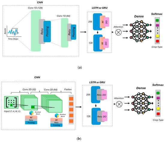
Figure 6.
Proposed four main architectures for time-series classification: (a) 1D CNN approach (integrated with either LSTM or GRU) that processes sequential feature vectors, and (b) 2D CNN approach (with LSTM or GRU) designed for spatiotemporal patches.
The 1D CNN + LSTM/GRU models process time-series spectral data using a combination of 1D convolutional layers and LSTM/GRU layers. The architecture begins with two Conv1D layers (128 and 64 filters, kernel size of 7) to extract local temporal features, followed by local max-pooling and dropout layers to reduce dimensionality and prevent overfitting. The extracted features are fed into two stacked LSTM or GRU layers (128 and 64 units), which capture long-term dependencies. Batch normalization and dropout layers are applied after each RNN layer for regularization. An attention mechanism is used to focus on critical time steps, and the output is pooled using local max pooling. The final dense layers refine the features before the softmax output layer classifies the input into crop types.
The 2D CNN + LSTM/GRU hybrid models are designed to process spatial-temporal data, such as time series of spatial image patches, by combining time-distributed 2D convolutional layers and recurrent layers. The model begins with TimeDistributed 2D CNN layers consisting of Conv2D layers (with 32 and 64 filters) applied independently at each step to extract spatial features such as edges, textures, and field structures. A residual block is a design pattern originally popularized by ResNet [84] that introduces a skip (shortcut) connection from the input of the block to its output. Residual connections help mitigate the vanishing gradient problem, allowing gradients to flow directly from later layers to earlier layers [85]. Batch normalization, Relu, and pooling are applied after each convolutional layer to improve training stability. The output is flattened using a TimeDistributed flattening layer, which prepares the spatial features for input into the recurrent layers. The LSTM or GRU layers follow, where the first layer has 256 units, capturing long-term temporal dependencies. A second LSTM or GRU layer with 128 units further refines the temporal context. Dropout layers are applied after each RNN layer to reduce overfitting. The resulting temporal features are passed through two dense layers (128 and 64 units) with ReLU activation and dropout for feature refinement. Finally, the model outputs class probabilities through a softmax layer, classifying the input into different crop types. The model is compiled using the Adam optimizer and sparse categorical cross-entropy loss, ensuring robust learning from spatial and temporal data.
2.6.4. Sample Design and Classifier Training
For the 1D CNN + LSTM/GRU models, the input data consists of 2071 samples with a shape of (2071, 11, 14), representing 11-time steps and 14 spectral features per sample, such as spectral bands or vegetation indices. For the 2D CNN + LSTM/GRU model, 16 × 16 spatial patches are extracted for each polygon over 11-time steps, with 14 features. The batch sizes of 16, 32, 64, and 256 are tested to identify the optimal batch size for efficient training. To address class imbalance, class weights are applied during training, ensuring minority crop classes receive adequate focus. To address class imbalance, we re-weight the loss using scikit-learn’s balanced class weights, computed on the training split and supplied via Keras’ class_weight argument. This preserved the original spectral temporal signatures while proportionally emphasizing underrepresented crop types. All models are compiled using the Adam optimizer and the sparse categorical cross-entropy loss function [86], suitable for multi-class crop classification [42,87]. Training is conducted for a maximum of 100 epochs, with early stopping monitoring the validation loss and halting training if no improvement is observed for 5 consecutive epochs. A ReduceLROnPlateau callback dynamically reduces the learning rate by a factor of 0.5 if the validation loss plateaus, promoting smoother convergence. Model checkpoints ensure that the best-performing model is saved for evaluation. This robust training setup efficiently captures temporal and spatial crop patterns while mitigating overfitting and handling class imbalance.
2.7. Evaluation Model
To evaluate the performance of the proposed 1D CNN + LSTM/GRU and 2D CNN + LSTM/GRU models, overall accuracy (OA) and F1 macro are employed as the primary metrics for assessing overall model performance. For per-class analysis, precision, recall, and F1 score are additionally reported to assess classification performance at the crop-type level. Precision measures how many of the predicted crop samples were correctly classified, indicating the accuracy of positive predictions made by the model. Recall assesses the model’s ability to identify all actual instances of a crop type within the dataset, ensuring it captures the correct samples. The F1 score, being the harmonic mean of precision and recall, provides a balanced assessment, particularly in the presence of class imbalance. Overall accuracy calculates the proportion of correctly classified samples across all crop types, offering a comprehensive view of the model’s performance. Additionally, confusion matrices are generated to help analyze misclassification patterns and identify areas where the model may need improvement. The formulas for overall accuracy and F1 macro are provided below:
N samples with true labels and predictions
K = the number of classes
3. Results
3.1. Performance Analysis of Classification Models
This section presents a detailed comparative analysis of the performance metrics, specifically Overall Accuracy (OA) and F1 macro, of four distinct classification models that combine Convolutional Neural Networks (CNNs) with Recurrent Neural Networks (RNNs). Table 4 summarizes classification results across all models. Additionally, Figure 7 illustrates the classification maps generated by each model, providing a qualitative assessment of their spatial prediction capabilities.
Table 4.
Comparative overall accuracy (OA), ± standard deviation, and F1 macro of CNN-RNN Models.
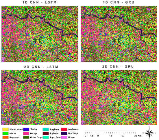
Figure 7.
Classification maps generated by each model.
The results from Table 4 clearly demonstrate that models incorporating a 2D CNN framework outperform their 1D CNN counterparts. The highest Overall Accuracy was achieved by the 2D CNN-GRU model, with an accuracy of 99.12% and an F1 macro of 99.14%, closely followed by the 2D CNN-LSTM model with 98.51% accuracy and an identical F1 macro. On the other hand, the 1D CNN models displayed relatively lower performance, with the 1D CNN-GRU model outperforming the 1D CNN-LSTM, obtaining an OA of 93.46% and an F1 of 93.21% versus 92.54% and 92.11%, respectively.
Figure 7 visually supports the qualitative findings, underscoring the significant performance margin between the 1D and 2D CNN-based models. This observation suggests that incorporating spatial context through 2D convolutional operations substantially enhances classification performance, particularly in complex agricultural regions where spatial relationships are critical. Comparison of computational efficiency under identical settings (batch size = 32; Intel i7-12700, 32 GB RAM, NVIDIA RTX 3060). Single run training time to convergence was 00:04:12 for 1D CNN-LSTM, 00:03:10 for 1D CNN-GRU, 01:13:45 for 2D CNN-LSTM, 01:10:23 for 2D CNN-GRU. Inference on the same test workload required 00:35:42 (1D CNN-LSTM), 00:23:37 (1D CNN-GRU), 02:57:42 (2D CNN-LSTM), and 02:37:13 (2D CNN-GRU). As expected, 2D models incur higher costs than 1D due to spatial convolutions, while GRU variants are consistently faster than LSTM at the same architecture capacity. We repeated each model five times with different random seeds and summarized performance as OA (mean ± SD) and macro-F1 across runs. To test differences, we ran two-sided paired t-tests on OA across random seeds (df = 4). The results (Table 5) across five runs confirmed that all pairwise model comparisons were statistically significant (p < 0.05), with 2D CNN-LSTM and 2D CNN-GRU showing superior performance over 1D CNN-LSTM and 1D CNN-GRU.
Table 5.
A paired t-test was performed to evaluate the statistical significance of differences between models for df = 4. Significance is indicated by p ≤ 0.05.
3.2. Evaluation Metrics and Per-Class Analysis
We employed confusion matrices and standard classification metrics, precision, recall, and F1-score on a per-class basis. These metrics help assess how well each model performs across individual crop classes. The confusion matrices for all four models, 1D CNN-LSTM, 1D CNN-GRU, 2D CNN-LSTM, and 2D CNN-GRU, are presented in Figure 8. The highest accuracies were observed for the most dominant classes, such as Wheat and Maize, which consistently appeared along the diagonal of the matrices across all models, indicating correct predictions.
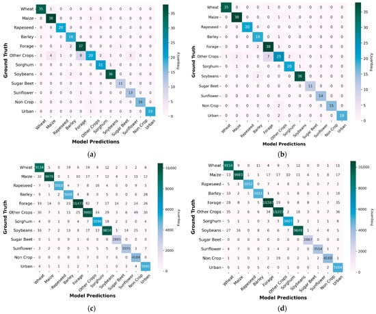
Figure 8.
Confusion matrices for all four models (a) 1D CNN-LSMT (b) 1D CNN-GRU (c) 2D CNN-LSTM (d) 2D CNN-GRU.
The 1D CNN-LSTM model demonstrated solid performance overall, particularly on major crop types. However, some confusion was noted between classes with similar spectral and temporal profiles, such as Rapeseed and Barley. Likewise, classes such as Forage and Other Crops occasionally overlapped, highlighting challenges in modeling subtler class differences based on temporal patterns alone. The 1D CNN-GRU model showed comparable behavior but with slightly improved separation in a few problematic categories, suggesting the GRU’s ability to better capture temporal dependencies in certain contexts.
When spatial information was integrated through 2D convolutions, model performance improved. The 2D CNN-LSTM model demonstrated enhanced discrimination in classes that previously exhibited higher confusion. Classes like Sugar Beet, Sunflower, and Non-Crop saw clearer separation from neighboring classes, likely due to the spatial patterns being better captured in the input features. The most refined results were observed with the 2D CNN-GRU model, which not only maintained high performance on the dominant classes but also significantly improved the accuracy of minority and visually complex classes. This model showed fewer off-diagonal misclassifications and achieved more consistent predictions across all categories.
Overall, the progression from 1D to 2D models, and from LSTM to GRU-based architectures, illustrates the importance of leveraging both spatial and temporal information for complex crop classification tasks. The confusion matrices and class-wise metrics (Table 5) collectively highlight the robustness and generalizability of the 2D CNN-GRU model, particularly in handling diverse and spectrally overlapping crop types.
3.3. Learning Curves and Convergence Behavior
For training dynamics and generalization ability of the proposed models, we analyzed the learning curves for both accuracy and loss across training epochs. Figure 9 shows the training dynamics of two sequential architectures: 1D CNN-LSTM and 1D CNN-GRU. Subplot (a) presents the training and validation accuracy for the 1D CNN-LSTM model, while subplot (b) shows its corresponding loss curve. Subplots (c) and (d) display the accuracy and loss curves, respectively, for the 1D CNN-GRU model.
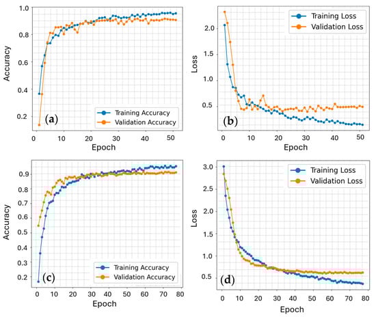
Figure 9.
Training and Validation curves (a) training and validation accuracy curves 1D CNN-LSMT (b) training and validation loss curves 1D CNN-LSTM (c) training and validation accuracy curves 1D CNN-GRU (d) training and validation loss curves 1D CNN-GRU.
The 1D CNN-LSTM model Figure 9a demonstrates consistent upward trend in both training and validation accuracy, with the curves closely aligned by the later epochs. This indicates that the model is not only learning effectively but also generalizing well to unseen data. In the corresponding loss curve Figure 9b, a steady decline in training loss is observed, while the validation loss initially follows a similar trajectory before plateauing and exhibiting minor fluctuations.
Similarly, the 1D CNN-GRU model Figure 9c showed an improvement in both training and validation accuracy during the initial epochs, followed by gradual convergence. Interestingly, the validation accuracy occasionally surpasses the training accuracy, which may reflect effective regularization and model robustness. The loss curve for 1D CNN-GRU Figure 9d confirms this behavior, with both training and validation losses decreasing in parallel and showing minimal divergence, pointing to a stable learning process and strong generalization.
Continuing with the learning curves of the 2D CNN-based models, Figure 10 illustrates the training and validation performance for 2D CNN-LSTM and 2D CNN-GRU architectures. Subplots (a) and (b) represent the accuracy and loss curves for the 2D CNN-LSTM model, while (c) and (d) show the corresponding plots for the 2D CNN-GRU model.
Figure 10.
Training and Validation curves (a) training and validation accuracy curves21D CNN-LSMT (b) training and validation loss curves 2D CNN-LSTM (c) training and validation accuracy curves 2D CNN-GRU (d) training and validation loss curves 2D CNN-GRU.
The 2D CNN-LSTM model Figure 10a demonstrates a smooth and steady increase in both training and validation accuracy, with the validation curve consistently tracking above the training curve throughout most of the training process. This suggests not only efficient learning but also an excellent ability to generalize, as the model performs slightly better on unseen data. The associated loss curve Figure 10b further confirms this trend, with both training and validation losses decreasing steadily and maintaining close alignment, shows a stable and robust learning without signs of overfitting.
A similar pattern is observed in the 2D CNN-GRU model Figure 10c, which shows even more rapid convergence in validation accuracy compared to training. The validation curve remains above the training curve for most of the training epochs, reflecting strong generalization performance. The loss curve in Figure 10d shows this behavior, with both training and validation loss exhibiting a sharp decline early on and then gradually tapering off with very minimal fluctuation. The tight coupling between the two curves further suggests that the GRU architecture, when combined with 2D convolutions, is particularly effective at learning spatial-temporal representations with minimal overfitting.
Among all models, the 2D CNN-GRU achieved the best overall performance, showing the highest validation accuracy and the lowest, most stable loss. The 2D CNN-LSTM also performed well, with closely aligned training and validation curves. In contrast, the 1D models converged more slowly and showed minor fluctuations in validation loss, with the 1D CNN-GRU slightly outperforming the 1D CNN-LSTM in generalization. Overall, incorporating spatial features through 2D convolutions, especially with GRU, led to more robust and consistent learning.
4. Discussion
4.1. Performance Comparison of Classification Models
To assess the effectiveness of our proposed CNN-RNN hybrid architectures for crop classification, we compared their performance with previously published models in the literature. Figure 11 graph clearly highlights that our CNN-RNN-based architecture models outperform existing 1D CNN, 2D CNN, and RNN integration approaches in terms of overall accuracy (OA) and F1.
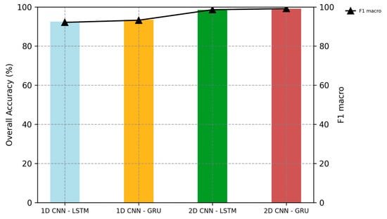
Figure 11.
Graphical comparison of the OA and F1 across all models.
In previous studies, [58] reported classification accuracies using Sentinel-2 imagery with conventional 1D CNN, LSTM, and GRU models, achieving OA values of 86.25%, 86.18%, and 81.67%, respectively. When they combined LSTM and GRU with 1D CNN, the performance slightly improved to 85.75% and 85.61%, indicating modest gains through hybrid architectures. In another work by [46], a standalone LSTM model achieved an accuracy of 86.23% for land cover classification, while [88] explored 1D CNN for satellite-based crop classification and obtained 89.5% using a 1D CNN and 93.7% with a 1D CNN-GRU hybrid. These results align with our findings, where the 1D CNN-GRU model outperformed the 1D CNN-LSTM variant, achieving an OA of 93.46%.
Our own experiments with 1D CNN-LSTM and 1D CNN-GRU yielded higher accuracies of 92.54% and 93.46%, respectively, which already showing improved performance due to optimized hybridization and training strategies. However, recognizing the limitations of 1D temporal-only modeling, we introduced spatial context by incorporating 2D convolutions before the recurrent layers. This allowed the network to extract spatial patterns alongside temporal dynamics, addressing the spatial heterogeneity common in satellite imagery. For comparison, [69] employed 2D CNN and achieved an OA of 94.76%.
In another previous study by [89], the use of standalone 2D CNN and LSTM models, as well as a combined 2D CNN-BiLSTM architecture, achieved overall accuracies of 92.54%, 93.90%, and 96.59%, respectively, though these results were obtained in a relatively small study area. In our study, we extend this design with long-term recurrent dependencies via LSTM and GRU modules using spectral and near-infrared and red edge-based vegetation indices of Sentinel-2 data, along with iterative training strategies. This even led to greater performance gains, with the 2D CNN-LSTM reaching 98.51% and the 2D CNN-GRU achieving 99.12% OA with corresponding F1 scores of 99.14%. Recent studies have demonstrated high accuracy in crop classification using advanced deep learning methods. Reference [90] used raw spectral bands and vegetation indices in combination with an RNN-CNN architecture enhanced by an attention mechanism, achieving 95.86% overall accuracy. Similarly, another study [56] reported an accuracy of 96.50% for land cover and crop classification using an R-CNN architecture. Reference [91] tested RF, SVM, Xgboost alongside a deep learning model PSETAE, using red-edge indices and raw Sentinel-2 bands, with Xgboost performing best at 95.49%. In contrast, our proposed framework, which integrates 1D and 2D CNN with LSTM/GRU, attains higher accuracy than these previous approaches. Reference [44] reported a TempCNN training time of 1 h 06 min at batch size 32, which is comparable to our 1 h 13 min. In [88], a CNN-GRU required 656 s/epoch, whereas our 2D CNN-GRU trains in 146 s/epoch on our hardware, demonstrating better calculation efficiency.
These results clearly outperform previous works and confirm the benefits of combining 2D spatial features with long-term temporal modeling. The performance improvement can be attributed to the deeper integration of spatial and temporal patterns, enhanced by the long-term memory capabilities of LSTM and GRU units. In summary, our findings show that transitioning from 1D CNN-RNN models to 2D CNN-based hybrid architectures leads to a substantial increase in classification performance. The 2D CNN-GRU stands out as the most effective model, offering both high accuracy and stable generalization, setting a new benchmark for crop mapping using time-series satellite data.
4.2. Performance Comparison of Per-Class Analysis
Figure 12 provides a comparative overview of precision, recall, and F1-score across all target classes for each of the CNN-RNN model combinations. Most crop categories demonstrated consistently high performance, particularly major classes such as Winter Wheat, Maize, and Soybeans, where F1-scores approached or exceeded 0.95 in all models. However, the Other Crops category consistently showed comparatively lower precision and recall values across all models. This class has a heterogeneous mix of minor crops and vegetables, often grown under artificial sheds. Such diversity introduces spectral heterogeneity, making it difficult for the models to learn a consistent feature representation. Additionally, the presence of built-up elements within or surrounding these plots, such as greenhouses and sheds, complicates the classification task due to spectral overlap with non-crop and built-up land-use types. Another factor is the absence of fixed crop calendars for the Other Crops category, unlike major seasonal crops, which follow well-defined sowing and harvesting periods. Since the satellite imagery used in this study was acquired during the winter crop season, it may not have fully captured the phenological signatures of certain minor or off-season crops, which can lead to further misclassification. To address this, future work could benefit from integrating ancillary data sources such as crop calendars or phenological profiles specific to minor and mixed crop types.
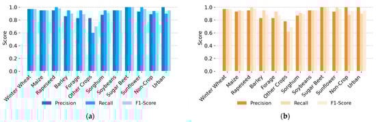
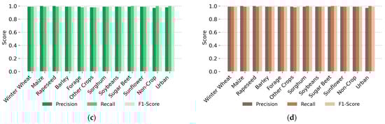
Figure 12.
Comparative overview of precision, recall, and F1-score for each crop class across all four models: (a) 1D CNN-LSTM, (b) 1D CNN-GRU, (c) 2D CNN-LSTM, (d) 2D CNN-GRU.
4.3. Visual Comparison of Crop Classification Results
Figure 13 shows a visual comparison of crop classification results across all four model architectures 1D CNN-LSTM, 1D CNN-GRU, 2D CNN-LSTM, and 2D CNN-GRU, alongside the corresponding false color Sentinel-2 imagery. These maps provide details on how spatial and temporal modeling impacts the quality and clarity of classification outputs.
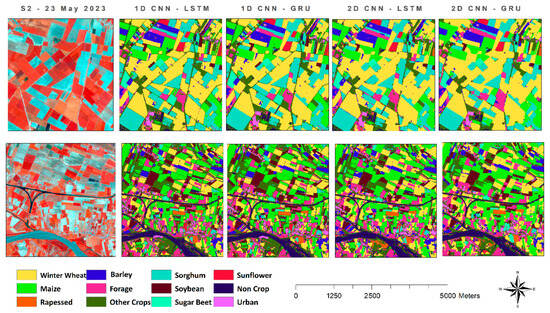
Figure 13.
Comparison of zoomed-in areas from the classification maps generated by the four models, highlighting differences in spatial detail and classification performance.
1D CNN are particularly effective in processing remote sensing data due to their ability to focus on spectral features across time [92,93]. However, a key limitation of 1D CNN is their inability to account for spatial context, as they primarily focus on spectral data, and may ignore spatial features such as texture, shape, and field-level structures information, which can be a limitation in applications where spatial context is crucial [94]. This limitation is evident in the visual results, where 1D CNN-LSTM and 1D CNN-GRU maps exhibit missing or noisy pixels within homogeneous crop fields, and field boundaries often appear blurred or fragmented.
In contrast, 2D CNN are designed to extract spatial features, which is particularly advantageous when working with high-resolution satellite imagery [95,96]. The addition of 2D convolutional layers before the recurrent units allows the network to learn not only spectral-temporal patterns but also texture, shape, and field-level structures, which are crucial in agricultural mapping. This is clearly reflected in the maps produced by the 2D CNN-LSTM and 2D CNN-GRU models, where crop fields appear more continuous, well-defined, and accurately segmented. Boundaries between adjacent fields are more sharply identified. These improvements are especially important where an accurate delineation of field edges is required. Among the models, 2D CNN-GRU delivered the most visually consistent and accurate results. This aligns with its superior performance in both accuracy and F1-score. The combination of spatial learning through 2D convolutions and the long-term temporal modeling capacity of GRU provides a balanced architecture for capturing the complexity of crop dynamics and spatial variability. In summary, while 1D CNN demonstrate strong performance for spectral-focused tasks, their limitations in spatial understanding can reduce classification quality in applications where field texture and boundary recognition are critical. By contrast, 2D CNN-based models offer a more comprehensive approach, integrating both spectral and spatial dimensions, which results in significantly enhanced visual and structural quality in crop classification tasks.
4.4. Impact of Pooling Types and Residual Block Architectures
We evaluated the architectural influences on model performance and analyzed the impact of different pooling strategies and the inclusion of residual blocks within the model networks. Figure 14 shows the impact of pooling layers and residual blocks on the overall accuracy of classification models. Our experiments demonstrated that changing the pooling approach by replacing local max pooling [97], average [98], and global average pooling [84] had a negligible effect on the classification performance across all models. This suggests that the learned features, particularly in the convolutional stages, were sufficiently robust and invariant to the pooling choices. In previous studies, [44] observed that the use of pooling layers could reduce overall accuracy. However, in our approach, we incorporated local max pooling to lower computations, faster training, and to prevent overfitting without compromising on overall classification accuracy.
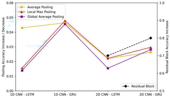
Figure 14.
Showing the impact of pooling choices and residual block influence on overall accuracy for all models.
The use of residual block architectures introduced an improvement in the performance of the 2D CNN-based models. Incorporating residual connections in both the 2D CNN-LSTM and 2D CNN-GRU models significantly enhanced the overall classification accuracy. These improvements can be attributed to the ability of residual blocks to preserve low-level spatial information and facilitate better gradient flow during training [99]. Therefore, it can enable deeper convolutional representations without the typical degradation issues [100]. The results in Figure 13 indicate that using residual learning for spatiotemporal classification tasks using satellite imagery has an advantage. While the choice of pooling strategy may be flexible, the integration of residual blocks is a more critical architectural decision, leading to measurable gains in model accuracy and robustness.
5. Conclusions
In conclusion, this study introduced a spatio-temporal deep learning approach for crop classification using hybrid CNN-RNN architectures. We explored the potential of Sentinel-2 spectral bands and NIR and red-edge-based vegetation indices by combining spatial and spectral features extracted through 1D And 2D CNNs with temporal patterns captured by LSTM and GRU networks. We conducted a comprehensive comparison of four model configurations. The findings demonstrated the superior performance of the 2D CNN-GRU model, which outperformed all others, followed closely by the 2D CNN-LSTM model. In contrast, the 1D CNN-based RNN models, though effective in capturing spectral-temporal patterns, showed reduced accuracy due to the absence of spatial context. The proposed 2D CNN-GRU model achieved superior classification results, with an overall accuracy of 99.12%, an F1 score of 99.14%, and visually coherent crop maps that effectively captured field-level textures and boundaries. These results emphasized the significance of incorporating spatial context alongside temporal modeling to enhance classification robustness and map quality, especially in heterogeneous agricultural landscapes. Overall, this study demonstrates the effectiveness of combining 2D CNN with GRU for satellite-based crop classification and sets a benchmark for future research. The results indicated that integration of spatial and temporal learning in remote sensing models encourages continued exploration into multi-source data fusion and advanced temporal modeling techniques to further improve crop mapping accuracy. The models were trained using data from a specific region and cropping season; therefore, future research is needed to study their generalizability to other areas. Moreover, more research is needed to further investigate issues related to data collection, computational costs, and ancillary data integration. In fact, the predictive accuracy depends highly on the availability of clean, labeled training data, which can be challenging and costly to obtain. Additionally, while 2D CNN improved spatial detail, they require significant computational resources, which may restrict scalability. Finally, the use of only Sentinel-2 time series data may benefit from the integration with auxiliary information like crop calendars, soil data, or weather, which could help improve the classification of spectrally complex or minor crop classes.
Author Contributions
Conceptualization, R.T. and D.T.; methodology, R.T., P.T. and D.T.; software, R.T.; validation, R.T., P.T. and D.T.; formal analysis, R.T.; investigation, R.T.; resources, P.T. and D.T.; data curation, R.T.; writing—original draft preparation, R.T.; writing—review and editing, R.T., P.T. and D.T.; visualization, R.T.; supervision, P.T. and D.T.; project administration, P.T. and D.T.; funding acquisition, P.T. and D.T. All authors have read and agreed to the published version of the manuscript.
Funding
This study was carried out within the Agritech National Research Center and received funding from the European Union Next-GenerationEU (PIANO NAZIONALE DI RIPRESA E RESILIENZA (PNRR)—MISSIONE 4 COMPONENTE 2, INVESTIMENTO 1.4—D.D. 1032 17/06/2022, CN00000022). This manuscript reflects only the authors’ views and opinions, neither the European Union nor the European Commission can be considered responsible for them.
Informed Consent Statement
The authors used ChatGPT (OpenAI, GPT-4, 2024 version) for grammar correction purposes and to improve the English form. After using such tool, the authors reviewed, edited, and verified all the content as needed and take full responsibility for the content of this publication.
Data Availability Statement
Data will be made available on request.
Conflicts of Interest
The authors declare no conflicts of interest.
Abbreviations
The following abbreviations are used in this manuscript:
| Symbol | Meaning |
| CNN | Convolutional Neural Networks |
| RNN | Recurrent Neural Networks |
| 1D CNN | One-Dimensional Convolutional Neural Networks |
| 2D CNN | Two-Dimensional Convolutional Neural Networks |
| LSTM | Long Short-Term Memory |
| GRU | Gated Recurrent Unit |
| DL | Deep Learning |
| ML | Machine Learning |
| RF | Random Forest |
| SVM | Support Vector Machine |
| VI | Vegetation Indices |
| BOA | Bottom of the Atmosphere |
| RE | Red Edge |
| KNN | K-Nearest Neighbors Radial Basis Function |
References
- Harris, D.R.; Fuller, D.Q. Agriculture: Definition and overview. In Encyclopedia of Global Archaeology; Smith, C., Ed.; Springer: New York, NY, USA, 2014; pp. 104–113. [Google Scholar] [CrossRef]
- Petersen, B.; Snapp, S. What is sustainable intensification? Views from experts. Land Use Policy 2015, 46, 1–10. [Google Scholar] [CrossRef]
- FAO. Hunger and Food Insecurity. 2025. Available online: https://www.fao.org/hunger/en (accessed on 9 January 2025).
- FAO. FAOSTAT: Suite of Food Security Indicators. 2024. Available online: https://www.fao.org/faostat/en/#data/FS (accessed on 9 January 2025).
- Wijerathna-Yapa, A.; Pathirana, R. Sustainable agro-food systems for addressing climate change and food security. Agriculture 2022, 12, 1554. [Google Scholar] [CrossRef]
- Rehman, M.U.; Eesaar, H.; Abbas, Z.; Seneviratne, L.; Hussain, I.; Chong, K.T. Advanced drone-based weed detection using feature-enriched deep learning approach. Knowl.-Based Syst. 2024, 305, 112655. [Google Scholar] [CrossRef]
- United Nations. Transforming Our World: The 2030 Agenda for Sustainable Development. 2025. Available online: https://sdgs.un.org/2030agenda (accessed on 9 January 2025).
- Hegarty-Craver, M.; Polly, J.; O’neil, M.; Ujeneza, N.; Rineer, J.; Beach, R.H.; Lapidus, D.; Temple, D.S. Remote crop mapping at scale: Using satellite imagery and UAV-acquired data as ground truth. Remote Sens. 2020, 12, 1984. [Google Scholar] [CrossRef]
- Vizzari, M.; Lesti, G.; Acharki, S. Crop classification in Google Earth Engine: Leveraging Sentinel-1, Sentinel-2, European CAP data, and object-based machine-learning approaches. Geo-Spat. Inf. Sci. 2024, 28, 815–830. [Google Scholar] [CrossRef]
- Balsamo, G.; Agusti-Panareda, A.; Albergel, C.; Arduini, G.; Beljaars, A.; Bidlot, J.; Blyth, E.; Bousserez, N.; Boussetta, S.; Brown, A.; et al. Satellite and in situ observations for advancing global Earth surface modelling: A review. Remote Sens. 2018, 10, 2038. [Google Scholar] [CrossRef]
- Guo, H.; Fu, W.; Liu, G. Earth observation technologies and scientific satellites for global change. In Scientific Satellite and Moon-Based Earth Observation for Global Change; Springer: Singapore, 2019; pp. 263–281. [Google Scholar] [CrossRef]
- Stojanova, D.; Panov, P.; Gjorgjioski, V.; Kobler, A.; Džeroski, S. Estimating vegetation height and canopy cover from remotely sensed data with machine learning. Ecol. Inform. 2010, 5, 256–266. [Google Scholar] [CrossRef]
- Fang, H.; Liang, S.; Chen, Y.; Ma, H.; Li, W.; He, T.; Tian, F.; Zhang, F. A comprehensive review of rice mapping from satellite data: Algorithms, product characteristics and consistency assessment. Sci. Remote Sens. 2024, 10, 100172. [Google Scholar] [CrossRef]
- Mishra, H.; Mishra, D. Sustainable smart agriculture to ensure zero hunger. In Sustainable Development Goals: Technologies and Opportunities; CRC Press: Boca Raton, FL, USA, 2024; pp. 16–37. [Google Scholar]
- Aldana-Martín, J.F.; García-Nieto, J.; del Mar Roldán-García, M.; Aldana-Montes, J.F. Semantic modelling of earth observation remote sensing. Expert Syst. Appl. 2022, 187, 115838. [Google Scholar] [CrossRef]
- Karthikeyan, L.; Chawla, I.; Mishra, A.K. A review of remote sensing applications in agriculture for food security: Crop growth and yield, irrigation, and crop losses. J. Hydrol. 2020, 586, 124905. [Google Scholar] [CrossRef]
- Khanal, S.; Kc, K.; Fulton, J.P.; Shearer, S.; Ozkan, E. Remote sensing in agriculture—Accomplishments, limitations, and opportunities. Remote Sens. 2020, 12, 3783. [Google Scholar] [CrossRef]
- Gascon, F. Sentinel-2 for agricultural monitoring. In Proceedings of the 2018 IEEE International Geoscience and Remote Sensing Symposium (IGARSS), Valencia, Spain, 22–27 July 2018; pp. 8166–8168. [Google Scholar] [CrossRef]
- Zheng, Y.; Dong, W.; Yang, Z.; Lu, Y.; Zhang, X.; Dong, Y.; Sun, F. A new attention-based deep metric model for crop type mapping in complex agricultural landscapes using multisource remote sensing data. Int. J. Appl. Earth Obs. Geoinf. 2024, 134, 104204. [Google Scholar] [CrossRef]
- Drusch, M.; Del Bello, U.; Carlier, S.; Colin, O.; Fernandez, V.; Gascon, F.; Hoersch, B.; Isola, C.; Laberinti, P.; Martimort, P.; et al. Sentinel-2: ESA’s optical high-resolution mission for GMES operational services. Remote Sens. Environ. 2012, 120, 25–36. [Google Scholar] [CrossRef]
- Segarra, J.; Buchaillot, M.L.; Araus, J.L.; Kefauver, S.C. Remote sensing for precision agriculture: Sentinel-2 improved features and applications. Agronomy 2020, 10, 641. [Google Scholar] [CrossRef]
- Belgiu, M.; Csillik, O. Sentinel-2 cropland mapping using pixel-based and object-based time-weighted dynamic time warping analysis. Remote Sens. Environ. 2018, 204, 509–523. [Google Scholar] [CrossRef]
- Thomas, N.; Neigh, C.S.R.; Carroll, M.L.; McCarty, J.L.; Bunting, P. Fusion approach for remotely-sensed mapping of agriculture (FARMA): A scalable open source method for land cover monitoring using data fusion. Remote Sens. 2020, 12, 3459. [Google Scholar] [CrossRef]
- Coulibaly, S.; Kamsu-Foguem, B.; Kamissoko, D.; Traore, D. Deep learning for precision agriculture: A bibliometric analysis. Intell. Syst. Appl. 2022, 16, 200102. [Google Scholar] [CrossRef]
- Gawade, S.D.; Bhansali, A.; Chopade, S.; Kulkarni, U. Optimizing crop yield prediction with R2U-Net-AgriFocus: A deep learning architecture with leveraging satellite imagery and agro-environmental data. Expert Syst. Appl. 2025, 296, 128942. [Google Scholar] [CrossRef]
- Bantchina, B.B.; Gündoğdu, K.S.; Yazar, S.; Author, C. Crop type classification using Sentinel-2A-derived normalized difference red edge index (NDRE) and machine learning approach. Bursa Uludağ Üniversitesi Ziraat Fakültesi Derg. 2024, 38, 89–105. [Google Scholar] [CrossRef]
- Moumni, A.; Lahrouni, A. Machine learning-based classification for crop-type mapping using the fusion of high-resolution satellite imagery in a semiarid area. Scientifica 2021, 2021, 6613372. [Google Scholar] [CrossRef]
- Wang, X.; Zhang, J.; Xun, L.; Wang, J.; Wu, Z.; Henchiri, M.; Zhang, S.; Zhang, S.; Bai, Y.; Yang, S.; et al. Evaluating the effectiveness of machine learning and deep learning models combined time-series satellite data for multiple crop types classification over a large-scale region. Remote Sens. 2022, 14, 2341. [Google Scholar] [CrossRef]
- Kussul, N.; Lavreniuk, M.; Skakun, S.; Shelestov, A. Deep learning classification of land cover and crop types using remote sensing data. IEEE Geosci. Remote Sens. Lett. 2017, 14, 778–782. [Google Scholar] [CrossRef]
- Thorp, K.; Drajat, D. Deep machine learning with Sentinel satellite data to map paddy rice production stages across West Java, Indonesia. Sens. Environ. 2021, 265, 112679. [Google Scholar] [CrossRef]
- Wang, J.; Wang, P.; Tian, H.; Tansey, K.; Liu, J.; Quan, W. A deep learning framework combining CNN and GRU for improving wheat yield estimates using time series remotely sensed multi-variables. Comput. Electron. Agric. 2023, 206, 107705. [Google Scholar] [CrossRef]
- Venkatanaresh, M.; Kullayamma, I. A new approach for crop type mapping in satellite images using hybrid deep capsule auto encoder. Knowl.-Based Syst. 2022, 256, 109881. [Google Scholar] [CrossRef]
- Saini, R. Integrating vegetation indices and spectral features for vegetation mapping from multispectral satellite imagery using AdaBoost and Random Forest machine learning classifiers. Geomat. Environ. Eng. 2023, 17, 57–74. [Google Scholar] [CrossRef]
- Amankulova, K.; Farmonov, N.; Mukhtorov, U.; Mucsi, L. Sunflower crop yield prediction by advanced statistical modeling using satellite-derived vegetation indices and crop phenology. Geocarto Int. 2023, 38, 2197509. [Google Scholar] [CrossRef]
- Sitokonstantinou, V.; Papoutsis, I.; Kontoes, C.; Arnal, A.L.; Andrés, A.P.A.; Zurbano, J.A.G. Scalable parcel-based crop identification scheme using Sentinel-2 data time-series for the monitoring of the Common Agricultural Policy. Remote Sens. 2018, 10, 911. [Google Scholar] [CrossRef]
- Gao, Y.; Zhao, Z.; Shang, G.; Liu, Y.; Liu, S.; Yan, H.; Chen, Y.; Zhang, X.; Li, W. Optimal feature selection and crop extraction using random forest based on GF-6 WFV data. Int. J. Remote Sens. 2024, 45, 7395–7414. [Google Scholar] [CrossRef]
- Kang, Y.; Meng, Q.; Liu, M.; Zou, Y.; Wang, X. Crop classification based on red edge features analysis of GF-6 WFV data. Sensors 2021, 21, 4328. [Google Scholar] [CrossRef]
- Adrian, J.; Sagan, V.; Maimaitijiang, M. Sentinel SAR-optical fusion for crop type mapping using deep learning and Google Earth Engine. ISPRS J. Photogramm. Remote Sens. 2021, 175, 215–235. [Google Scholar] [CrossRef]
- Du, Z.; Yang, J.; Ou, C.; Zhang, T. Smallholder crop area mapped with a semantic segmentation deep learning method. Remote Sens. 2019, 11, 888. [Google Scholar] [CrossRef]
- Song, W.; Feng, A.; Wang, G.; Zhang, Q.; Dai, W.; Wei, X.; Hu, Y.; Amankwah, S.O.Y.; Zhou, F.; Liu, Y. Bi-objective crop mapping from Sentinel-2 images based on multiple deep learning networks. Remote Sens. 2023, 15, 3417. [Google Scholar] [CrossRef]
- Ofori-Ampofo, S.; Pelletier, C.; Lang, S. Crop type mapping from optical and radar time series using attention-based deep learning. Remote Sens. 2021, 13, 4668. [Google Scholar] [CrossRef]
- Zhong, L.; Hu, L.; Zhou, H. Deep learning based multi-temporal crop classification. Sens. Environ. 2019, 221, 430–443. [Google Scholar] [CrossRef]
- Ienco, D.; Interdonato, R.; Gaetano, R.; Ho Tong Minh, D. Combining Sentinel-1 and Sentinel-2 satellite image time series for land cover mapping via a multi-source deep learning architecture. ISPRS J. Photogramm. Remote Sens. 2019, 158, 11–22. [Google Scholar] [CrossRef]
- Pelletier, C.; Webb, G.I.; Petitjean, F. Temporal convolutional neural network for the classification of satellite image time series. Remote Sens. 2019, 11, 523. [Google Scholar] [CrossRef]
- Feng, F.; Gao, M.; Liu, R.; Yao, S.; Yang, G. A deep learning framework for crop mapping with reconstructed Sentinel-2 time series images. Comput. Electron. Agric. 2023, 213, 108227. [Google Scholar] [CrossRef]
- Ienco, D.; Gaetano, R.; Dupaquier, C.; Maurel, P. Land cover classification via multitemporal spatial data by deep recurrent neural networks. IEEE Geosci. Remote Sens. Lett. 2017, 14, 1685–1689. [Google Scholar] [CrossRef]
- Krizhevsky, A.; Sutskever, I.; Hinton, G.E. ImageNet classification with deep convolutional neural networks. Adv. Neural Inf. Process. Syst. 2012, 25. Available online: https://papers.nips.cc/paper_files/paper/2012/hash/c399862d3b9d6b76c8436e924a68c45b-Abstract.html (accessed on 5 February 2025).
- Sher, M.; Minallah, N.; Frnda, J.; Khan, W. Elevating crop classification performance through CNN-GRU feature fusion. IEEE Access 2024, 12, 141013–141025. [Google Scholar] [CrossRef]
- Kattenborn, T.; Leitloff, J.; Schiefer, F.; Hinz, S. Review on convolutional neural networks (CNN) in vegetation remote sensing. ISPRS J. Photogramm. Remote Sens. 2021, 173, 24–49. [Google Scholar] [CrossRef]
- Liu, J.; Wang, T.; Skidmore, A.; Sun, Y.; Jia, P.; Zhang, K. Integrated 1D, 2D, and 3D CNNs enable robust and efficient land cover classification from hyperspectral imagery. Remote Sens. 2023, 15, 4797. [Google Scholar] [CrossRef]
- Hewamalage, H.; Bergmeir, C.; Bandara, K. Recurrent neural networks for time series forecasting: Current status and future directions. Int. J. Forecast. 2021, 37, 388–427. [Google Scholar] [CrossRef]
- Zaremba, W.; Sutskever, I.; Vinyals, O. Recurrent neural network regularization. arXiv 2014, arXiv:1409.2329. Available online: https://arxiv.org/abs/1409.2329 (accessed on 24 August 2025).
- Hochreiter, S.; Schmidhuber, J. Long short-term memory. Neural Comput. 1997, 9, 1735–1780. [Google Scholar] [CrossRef]
- Salem, F.M. Gated RNN: The gated recurrent unit (GRU) RNN. In Recurrent Neural Networks; Springer: Berlin/Heidelberg, Germany, 2022; pp. 85–100. [Google Scholar]
- Fan, X.; Chen, L.; Xu, X.; Yan, C.; Fan, J.; Li, X. Land cover classification of remote sensing images based on hierarchical convolutional recurrent neural network. Forests 2023, 14, 1881. [Google Scholar] [CrossRef]
- Mazzia, V.; Khaliq, A.; Chiaberge, M. Improvement in land cover and crop classification based on temporal features learning from Sentinel-2 data using recurrent-convolutional neural network (R-CNN). Appl. Sci. 2019, 10, 238. [Google Scholar] [CrossRef]
- Mou, L.; Bruzzone, L.; Zhu, X.X. Learning spectral–spatial features via a recurrent convolutional neural network for change detection in multispectral imagery. IEEE Trans. Geosci. Remote Sens. 2019, 57, 924–935. [Google Scholar] [CrossRef]
- Zhao, H.; Duan, S.; Liu, J.; Sun, L.; Reymondin, L. Evaluation of five deep learning models for crop type mapping using Sentinel-2 time series images with missing information. Remote Sens. 2021, 13, 2790. [Google Scholar] [CrossRef]
- Kerner, H.R.; Sahajpal, R.; Pai, D.B.; Skakun, S.; Puricelli, E.; Hosseini, M.; Meyer, S.; Becker-Reshef, I. Phenological normalization can improve in-season classification of maize and soybean: A case study in the central US Corn Belt. Sci. Remote Sens. 2022, 6, 100059. [Google Scholar] [CrossRef]
- Ghisellini, P.; Zucaro, A.; Viglia, S.; Ulgiati, S. Monitoring and evaluating the sustainability of the Italian agricultural system: An emergy decomposition analysis. Ecol. Model. 2014, 271, 132–148. [Google Scholar] [CrossRef]
- Azar, R.; Villa, P.; Stroppiana, D.; Crema, A.; Boschetti, M.; Brivio, P.A. Assessing in-season crop classification performance using satellite data: A test case in Northern Italy. Eur. J. Remote Sens. 2016, 49, 361–380. [Google Scholar] [CrossRef]
- Shojaeezadeh, S.A.; Elnashar, A.; Weber, T.K.D. A novel fusion of Sentinel-1 and Sentinel-2 with climate data for crop phenology estimation using machine learning. Sci. Remote Sens. 2025, 11, 100227. [Google Scholar] [CrossRef]
- Tufail, R.; Ahmad, A.; Javed, M.A.; Ahmad, S.R. A machine learning approach for accurate crop type mapping using combined SAR and optical time series data. Adv. Space Res. 2022, 69, 331–346. [Google Scholar] [CrossRef]
- Delogu, G.; Caputi, E.; Perretta, M.; Ripa, M.N.; Boccia, L. Using PRISMA hyperspectral data for land cover classification with artificial intelligence support. Sustainability 2023, 15, 13786. [Google Scholar] [CrossRef]
- Buda, M.; Maki, A.; Mazurowski, M.A. A systematic study of the class imbalance problem in convolutional neural networks. Neural Netw. 2018, 106, 249–259. [Google Scholar] [CrossRef]
- Jin, Y.; Liu, X.; Chen, Y.; Liang, X. Land-cover mapping using Random Forest classification and incorporating NDVI time-series and texture: A case study of central Shandong. Int. J. Remote Sens. 2018, 39, 8703–8723. [Google Scholar] [CrossRef]
- Sonobe, R.; Yamaya, Y.; Tani, H.; Wang, X.; Kobayashi, N.; Mochizuki, K. Crop classification from Sentinel-2-derived vegetation indices using ensemble learning. J. Appl. Remote Sens. 2018, 12, 026019. [Google Scholar] [CrossRef]
- Kang, Y.; Hu, X.; Meng, Q.; Zou, Y.; Zhang, L.; Liu, M.; Zhao, M. Land cover and crop classification based on red edge indices features of GF-6 WFV time series data. Remote Sens. 2021, 13, 4522. [Google Scholar] [CrossRef]
- Li, Q.; Tian, J.; Tian, Q. Deep learning application for crop classification via multi-temporal remote sensing images. Agriculture 2023, 13, 906. [Google Scholar] [CrossRef]
- Ndikumana, E.; Ho Tong Minh, D.; Baghdadi, N.; Courault, D.; Hossard, L. Deep recurrent neural network for agricultural classification using multitemporal SAR Sentinel-1 for Camargue, France. Remote Sens. 2018, 10, 1217. [Google Scholar] [CrossRef]
- Jogin, M.; Mohana, H.S.; Madhulika, M.S.; Divya, G.D.; Meghana, R.K.; Apoorva, S. Feature extraction using convolution neural networks (CNN) and deep learning. In Proceedings of the 2018 3rd IEEE International Conference on Recent Trends in Electronics, Information & Communication Technology (RTEICT), Bangalore, India, 18–19 May 2018; pp. 2319–2323. [Google Scholar] [CrossRef]
- Ding, W.; Abdel-Basset, M.; Alrashdi, I.; Hawash, H. Next generation of computer vision for plant disease monitoring in precision agriculture: A contemporary survey, taxonomy, experiments, and future direction. Inf. Sci. 2024, 665, 120338. [Google Scholar] [CrossRef]
- Hu, W.; Huang, Y.; Wei, L.; Zhang, F.; Li, H. Deep convolutional neural networks for hyperspectral image classification. J. Sens. 2015, 2015, 258619. [Google Scholar] [CrossRef]
- Zhao, H.; Chen, Z.; Jiang, H.; Jing, W.; Sun, L.; Feng, M. Evaluation of three deep learning models for early crop classification using Sentinel-1A imagery time series—A case study in Zhanjiang, China. Remote Sens. 2019, 11, 2673. [Google Scholar] [CrossRef]
- Ioffe, S.; Szegedy, C. Batch normalization: Accelerating deep network training by reducing internal covariate shift. In Proceedings of the 32nd International Conference on Machine Learning (ICML), Lille, France, 6–11 July 2015; pp. 448–456. Available online: https://proceedings.mlr.press/v37/ioffe15.html (accessed on 24 August 2025).
- Hinton, G.E.; Srivastava, N.; Krizhevsky, A.; Sutskever, I.; Salakhutdinov, R.R. Improving neural networks by preventing co-adaptation of feature detectors. arXiv 2012, arXiv:1207.0580. Available online: https://arxiv.org/abs/1207.0580 (accessed on 24 August 2025). [CrossRef]
- Boureau, Y.L.; Ponce, J.; LeCun, Y. A theoretical analysis of feature pooling in visual recognition. In Proceedings of the 27th International Conference on Machine Learning (ICML), Haifa, Israel, 21–24 June 2010. [Google Scholar]
- Krizhevsky, A.; Sutskever, I.; Hinton, G.E. ImageNet classification with deep convolutional neural networks. Commun. ACM 2017, 60, 84–90. [Google Scholar] [CrossRef]
- LeCun, Y.; Bottou, L.; Orr, G.B.; Müller, K.-R. Efficient Backprop. In Neural Networks: Tricks of the Trade; Orr, G.B., Müller, K.-R., Eds.; Springer: Berlin/Heidelberg, Germany, 1998; pp. 9–50. [Google Scholar] [CrossRef]
- Paoletti, M.E.; Haut, J.M.; Plaza, J.; Plaza, A. Deep learning classifiers for hyperspectral imaging: A review. ISPRS J. Photogramm. Remote Sens. 2019, 158, 279–317. [Google Scholar] [CrossRef]
- Lipton, Z.C.; Berkowitz, J.; Elkan, C. A critical review of recurrent neural networks for sequence learning. arXiv 2015, arXiv:1506.00019. Available online: https://arxiv.org/abs/1506.00019 (accessed on 24 August 2025). [CrossRef]
- Bakker, B. Reinforcement learning with long short-term memory. Adv. Neural Inf. Process. Syst. 2001, 14. [Google Scholar]
- Chung, J.; Gulcehre, C.; Cho, K.; Bengio, Y. Empirical evaluation of gated recurrent neural networks on sequence modeling. arXiv preprint 2014, arXiv:1412.3555. Available online: https://arxiv.org/abs/1412.3555 (accessed on 24 August 2025).
- He, K.; Zhang, X.; Ren, S.; Sun, J. Deep residual learning for image recognition. In Proceedings of the IEEE Conference on Computer Vision and Pattern Recognition (CVPR), Las Vegas, NV, USA, 27–30 June 2016; pp. 770–778. [Google Scholar] [CrossRef]
- Ashwini, B.; Kaur, M.; Singh, D.; Roy, S.; Amoon, M. Efficient skip connections-based residual network (ESRNet) for brain tumor classification. Diagnostics 2023, 13, 3234. [Google Scholar] [CrossRef]
- Zhang, Z.; Sabuncu, M.R. Generalized cross entropy loss for training deep neural networks with noisy labels. Adv. Neural Inf. Process. Syst. 2018, 31. Available online: https://proceedings.neurips.cc/paper_files/paper/2018/hash/13f3cf8c531952d72e5847c4183e6910-Abstract.html (accessed on 15 March 2025).
- Russwurm, M.; Körner, M. Temporal vegetation modelling using long short-term memory networks for crop identification from medium-resolution multispectral satellite images. Remote Sens. 2017, 9, 11–19. [Google Scholar]
- Garnot, V.S.F.; Landrieu, L.; Giordano, S.; Chehata, N. Time-space tradeoff in deep learning models for crop classification on satellite multi-spectral image time series. In Proceedings of the IGARSS 2019-2019 IEEE International Geoscience and Remote Sensing Symposium, Yokohama, Japan, 28 July–2 August 2019; pp. 6247–6250. [Google Scholar] [CrossRef]
- Kwak, G.H.; Park, M.G.; Park, C.W.; Lee, K.D.; Na, S.I.; Ahn, H.Y.; Park, N.W. Combining 2D CNN and bidirectional LSTM to consider spatio-temporal features in crop classification. Korean J. Remote Sens. 2019, 35, 681–692. [Google Scholar]
- Zhang, F.; Yin, J.; Wu, N.; Hu, X.; Sun, S.; Wang, Y. A dual-path model merging CNN and RNN with attention mechanism for crop classification. Eur. J. Agron. 2024, 159, 127273. [Google Scholar] [CrossRef]
- Tufail, R.; Tassinari, P.; Torreggiani, D. Assessing feature extraction, selection, and classification combinations for crop mapping using Sentinel-2 time series: A case study in northern Italy. Remote Sens. Appl. Soc. Environ. 2025, 38, 101525. [Google Scholar] [CrossRef]
- Justo, J.A.; Garrett, J.L.; Georgescu, M.-I.; Gonzalez-Llorente, J.; Ionescu, R.T.; Johansen, T.A. Sea-land-cloud segmentation in satellite hyperspectral imagery by deep learning. Remote Sens. 2023, 15, 1267. [Google Scholar] [CrossRef]
- Song, Y.; Zhang, Z.; Baghbaderani, R.K.; Wang, F.; Qu, Y.; Stuttsy, C.; Qi, H. Land cover classification for satellite images through 1D CNN. In Proceedings of the 2019 10th Workshop on Hyperspectral Image and Signal Processing: Evolution in Remote Sensing (WHISPERS), Amsterdam, The Netherlands, 24–26 September 2019. [Google Scholar]
- Cai, J.; Boust, C.; Mansouri, A. ATSFCNN: A novel attention-based triple-stream fused CNN model for hyperspectral image classification. Mach. Learn. Sci. Technol. 2024, 5, 015024. [Google Scholar] [CrossRef]
- Fırat, H.; Asker, M.E.; Hanbay, D. Classification of hyperspectral remote sensing images using different dimension reduction methods with 3D/2D CNN. Remote Sens. Appl. Soc. Environ. 2022, 25, 100694. [Google Scholar] [CrossRef]
- Saralioglu, E.; Gungor, O. Semantic segmentation of land cover from high-resolution multispectral satellite images by spectral-spatial convolutional neural network. Geocarto Int. 2022, 37, 657–677. [Google Scholar] [CrossRef]
- Ren, S.; He, K.; Girshick, R.; Sun, J. Faster R-CNN: Towards real-time object detection with region proposal networks. Adv. Neural Inf. Process. Syst. 2015, 28. Available online: https://papers.nips.cc/paper_files/paper/2015/hash/14bfa6bb14875e45bba028a21ed38046-Abstract.html (accessed on 4 March 2025).
- Bieder, F.; Sandkühler, R.; Cattin, P.C. Comparison of methods generalizing max- and average-pooling. arXiv 2021, arXiv:2103.01746. [Google Scholar] [CrossRef]
- Kwak, N.-J.; Shin, H.-J.; Yang, J.-S.; Song, T.-S. CNN applied modified residual block structure. J. Korea Multimed. Soc. 2020, 23, 803–811. [Google Scholar]
- Mohamed Yassin, W.; Faizal Abdollah, M.; Muslim, Z.; Ahmad, R.; Ismail, A. An emotion and gender detection using hybridized convolutional 2D and batch norm residual network learning. In Proceedings of the 2021 9th International Conference on Information Technology: IoT and Smart City, Guangzhou, China, 22–25 December 2021; pp. 79–84. [Google Scholar]


Disclaimer/Publisher’s Note: The statements, opinions and data contained in all publications are solely those of the individual author(s) and contributor(s) and not of MDPI and/or the editor(s). MDPI and/or the editor(s) disclaim responsibility for any injury to people or property resulting from any ideas, methods, instructions or products referred to in the content. |
© 2025 by the authors. Licensee MDPI, Basel, Switzerland. This article is an open access article distributed under the terms and conditions of the Creative Commons Attribution (CC BY) license (https://creativecommons.org/licenses/by/4.0/).