Deep Learning-Based Super-Resolution Reconstruction of a 1/9 Arc-Second Offshore Digital Elevation Model for U.S. Coastal Regions

Highlights

What are the main findings?

• This study proposed DEM-AMSSRN, an asymmetric multi-scale super-resolution network that effectively preserves both large-scale geomorphology and fine-scale terrain details in offshore DEM reconstruction.

What is the implication of the main finding?

• By incorporating region-level non-local modules, residual multi-scale blocks, and a custom hybrid loss function, our method achieves a significant RMSE reduction of up to 72.47%. Moreover, it facilitates the construction of USA_OD_2025, marking the first 1/9 arc-second high-resolution offshore DEM for U.S. coastal regions.

Abstract

High-resolution offshore digital elevation models (DEMs) are essential for coastal geomorphology, marine resource management, and disaster prevention. While deep learning-based super-resolution (SR) techniques have become a mainstream solution for enhancing DEMs, they often fail to maintain a balance between large-scale geomorphological structure and fine-scale topographic detail due to limitations in modeling spatial dependency. To overcome this challenge, we propose DEM-Asymmetric multi-scale super-resolution network (DEM-AMSSRN), a novel asymmetric multi-scale super-resolution network tailored for offshore DEM reconstruction. Our method incorporates region-level non-local (RL-NL) modules to capture long-range spatial dependencies and residual multi-scale blocks (RMSBs) to extract hierarchical terrain features. Additionally, a hybrid loss function combining pixel-wise, perceptual, and adversarial losses is introduced to ensure both geometric fidelity and visual realism. Experimental evaluations on U.S. offshore DEM datasets demonstrate that DEM-AMSSRN significantly outperforms existing GAN-based models, reducing RMSE by up to 72.47% (vs. SRGAN) and achieving 53.30 dB PSNR and 0.995056 SSIM. These results highlight its effectiveness in preserving both continental shelf-scale bathymetric patterns and detailed terrain textures. Using this model, we also constructed the USA_OD_2025, a 1/9 arc-second high-resolution offshore DEM for U.S. coastal zones, providing a valuable geospatial foundation for future marine research and engineering.

1. Introduction

The coastal zones of the United States are dynamic transition areas where terrestrial and marine systems interact, supporting diverse ecosystems while sustaining major economic activities. With nearly 40% of the U.S. population residing in these regions [1], accurate characterization of coastal topography has become increasingly critical for applications such as fisheries, shipping, and tourism, each contributing billions annually to the national economy [2,3]. In the face of climate change and sea-level rise, high-resolution DEMs are vital for flood modeling [4], storm surge simulation [5], and tsunami risk assessment [6], particularly when integrated into hydrodynamic models for compound hazard prediction [7].

However, current U.S. offshore DEM datasets, primarily at 1/3 arc-second (~10 m) resolution, are insufficient for applications requiring sub-meter accuracy [8]. Limitations stem from high costs, limited spatial coverage, and resolution constraints in data acquisition technologies—airborne LiDAR suffers from water clarity dependence and high operational cost [9], multibeam sonar is expensive and labor-intensive [10], and satellite-derived bathymetry remains limited by depth and accuracy [11]. These challenges are especially prominent in dynamic coastal settings (e.g., tidal inlets), which demand both fine spatial and temporal resolution.

Deep learning-based SR methods have the ability to mitigate these limitations by enhancing resolution without the prohibitive costs or environmental constraints of traditional techniques, offering learned models capable of reconstructing fine-scale terrain from coarse-resolution inputs [12]. Unlike interpolation methods, modern SR architectures utilize multi-level feature extraction and attention mechanisms to preserve complex geomorphological structures [13]. Yet, general-purpose SR methods often fall short in DEM-specific contexts, where maintaining hydrological consistency and geomorphological realism is critical [14].

Recent studies have adapted SR techniques for DEM enhancement. Demiray et al. modified EfficientNetV2 [15] for elevation data, improving extraction but limiting multi-scale representation [16]. Deng et al. introduced dual-residual attention mechanisms, though their focus on channel-wise features compromised spatial integrity [17]. Lin et al. and Han et al. proposed hybrid learning and parallel modules to address global-local feature balance [18,19]. Emerging approaches such as implicit neural networks [20], deep image prior-based methods [21], and UnTDIP [22], which adopts a U-Net [23] architecture, have also shown potential.

Despite these advancements, key challenges remain. Existing models struggle to simultaneously preserve large-scale structural coherence and localized terrain details, and their generalizability across diverse coastal typologies is limited. To address these gaps, we propose DEM-AMSSRN, an asymmetric multi-scale super-resolution network designed specifically for offshore DEM reconstruction. DEM-AMSSRN combines parallel processing streams for local detail and global context extraction and introduces a hybrid loss function to enforce both pixel-level accuracy and geomorphological plausibility. By significantly enhancing topographic resolution while maintaining computational efficiency, DEM-AMSSRN represents a transformative resource for advancing marine spatial planning and sustainable coastal development initiatives.

2. Dataset and Methods

2.1. Source of Dataset

The continuously updated digital elevation models (CUDEMs), developed by Amante, Love, and colleagues, represent a significant advancement in coastal geospatial data provision. This initiative delivers high-resolution DEMs encompassing all U.S. coastal regions, with particular emphasis on the critical land–sea interface. CUDEMs provide exceptional spatial resolution: offshore topobathymetric models at 1/9 arc-second (~3 m) and bathymetric models at 1/3 arc-second (~10 m), achieving a mean vertical accuracy of 0.12 m ± 0.75 m with an overall RMSE of 0.76 m [24]. These high-precision DEMs are critical for coastal flood inundation modeling, enabling accurate prediction of flood timing and extent, which significantly enhances community preparedness, event forecasting, and early warning system development. The project has released numerous regional sub-datasets (detailed in

Table 1. Sub-datasets of CUDEM with resolutions and data sources.

Source	Resolution (Arc-Second)	Data URL
CUDEM 1/9th CONUS: NAVD88	1/9	https://coast.noaa.gov/dataviewer/#/lidar/search/where:ID=8483 (accessed on 15 September 2025)
CUDEM 1/9th Hawaii: MSL	1/9	https://coast.noaa.gov/dataviewer/#/lidar/search/where:ID=9428 (accessed on 15 September 2025)
CUDEM 1/9th Puerto Rico: PRVD02	1/9	https://coast.noaa.gov/dataviewer/#/lidar/search/where:ID=9525 (accessed on 15 September 2025)
CUDEM 1/9th USVI: VIVD09	1/9	https://coast.noaa.gov/dataviewer/#/lidar/search/where:ID=9529 (accessed on 15 September 2025)
CUDEM 1/9th Guam: GUVD04	1/9	https://coast.noaa.gov/dataviewer/#/lidar/search/where:ID=9462 (accessed on 15 September 2025)
CUDEM 1/9th CNMI: NMVD03	1/9	https://coast.noaa.gov/dataviewer/#/lidar/search/where:ID=9560 (accessed on 15 September 2025)
CUDEM 1/9th American Samoa: ASVD02	1/9	https://coast.noaa.gov/dataviewer/#/lidar/search/where:ID=9460 (accessed on 15 September 2025)
CUDEM 1/3rd CONUS: NAVD88	1/3	https://coast.noaa.gov/dataviewer/#/lidar/search/where:ID=8580 (accessed on 15 September 2025)
CUDEM 1/3rd Hawaii: MSL	1/3	https://coast.noaa.gov/dataviewer/#/lidar/search/where:ID=9429 (accessed on 15 September 2025)
CUDEM 1/3rd Puerto Rico: PRVD02	1/3	https://coast.noaa.gov/dataviewer/#/lidar/search/where:ID=9524 (accessed on 15 September 2025)
CUDEM 1/3rd USVI: VIVD09	1/3	https://coast.noaa.gov/dataviewer/#/lidar/search/where:ID=9528 (accessed on 15 September 2025)
CUDEM 1/3rd Guam: GUVD04	1/3	https://coast.noaa.gov/dataviewer/#/lidar/search/where:ID=9463 (accessed on 15 September 2025)
CUDEM 1/3rd CNMI: NMVD03	1/3	https://coast.noaa.gov/dataviewer/#/lidar/search/where:ID=9561 (accessed on 15 September 2025)
CUDEM 1/3rd American Samoa: ASVD02	1/3	https://coast.noaa.gov/dataviewer/#/lidar/search/where:ID=9461 (accessed on 15 September 2025)

), comprising multi-resolution DEMs tailored to specific geographic regions. These datasets provide researchers and practitioners with localized, high-precision elevation data optimized for specialized applications and regional-scale analyses.

For this study, we utilized the CUDEM 1/9 arc-second CONUS: NAVD88 sub-dataset as our primary data source, which was selected for its comprehensive coverage of U.S. coastal regions. This sub-dataset contains 872 high-resolution offshore DEM tiles (each 8112 × 8112 pixels) covering the majority of the U.S. coastline.

To optimize computational efficiency while maintaining data representative diversity, we selected a subset of 60 DEM tiles from CUDEM. These tiles were chosen to represent characteristic coastal geomorphological features across the East, West, and Gulf coasts, ensuring that the training dataset encompasses a broad spectrum of coastal landscapes. This targeted selection enhances model generalizability while avoiding the excessive training time and potential convergence issues that processing all 872 tiles might entail. 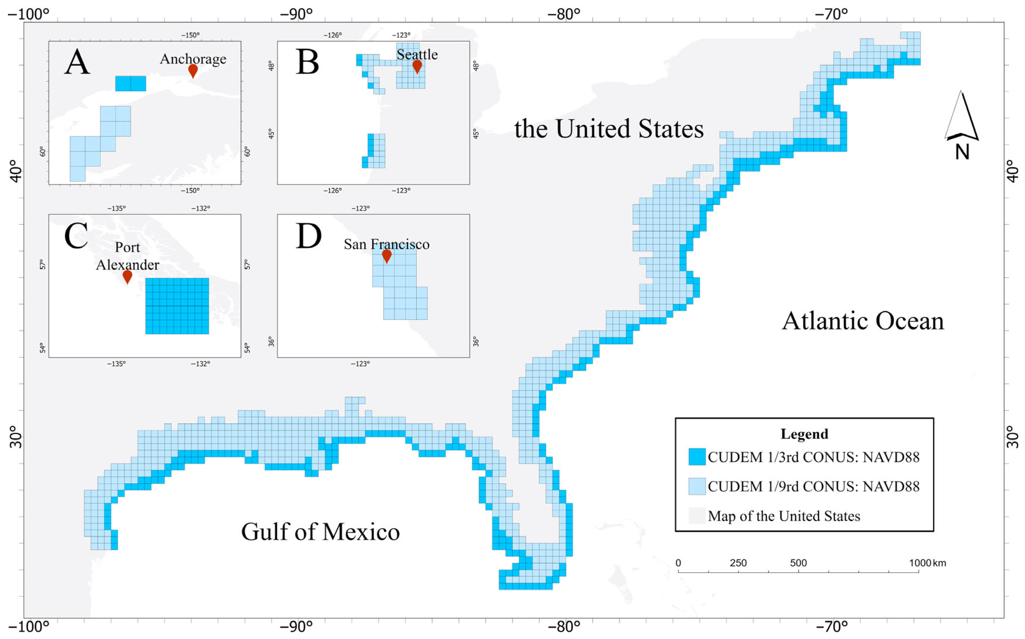Figure 1 maps the distribution of the full CUDEM dataset and highlights our 60-tile subset.

2.2. Dataset Processing

Normalization is essential for elevation data processing because raw elevation values vary widely across different terrains. Such variability can destabilize neural network training (causing gradient explosion or vanishing) and bias the model toward extreme values instead of meaningful features. We found that a global min–max normalization (scaling values to [0, 1]) introduces problems, especially in areas with complex topography. By compressing the entire elevation range, min–max normalization greatly reduces variance and can obscure subtle relief features. This can diminish the network’s ability to capture local topographic variations, lead to over-smoothed outputs (particularly in mountainous regions), and hinder effective gradient updates during training, potentially causing convergence issues.

To overcome these limitations, we adopted Z-score normalization, defined as follows:

$$\mathit{Z}={\displaystyle \frac{\mathit{x}-\mathit{\mu }}{\mathit{\sigma }}}$$

(1)

where $\mathit{x}$ represents the original elevation value, $\mathit{\mu }$ denotes the dataset mean, and $\mathit{\sigma }$ is the standard deviation. This approach offers three key advantages: (1) preservation of relative elevation differences through zero-centered, unit-variance transformation; (2) maintenance of local topographic features in extreme terrain (e.g., mountain ranges, canyons); and (3) prevention of dynamic range compression. The method additionally promotes faster network convergence by mitigating vanishing/exploding gradient risks while enhancing overall model stability and generalization capability.

We compared the effects of normalization methods on our data. As demonstrated in

Table 2. Elevation data statistics under different normalization methods (original, min–max, and Z-score).

Method	Mean	Variance
Original	−26.10	298.71
Min–max	0.5852	0.0585
Z-score	0.0000	1.0000

, the original elevation values exhibit a broad dynamic range (e.g., mean = −26.10, variance = 298.71), which poses challenges for neural network optimization. Min–max normalization compresses values into a [0, 1] range but drastically reduces variance (0.0585), potentially obscuring subtle topographic variations. In contrast, Z-Score standardization preserves the natural variability (mean = 0, variance = 1 by definition) and better retains meaningful topographic differences. Given these observations, the Z-score was chosen for all experiments.

The 60 DEM tiles were systematically divided into training (50 tiles) and validation (10 tiles) datasets. Each high-resolution training tile (8112 × 8112) was divided into 352,800 patches of 96 × 96 pixels (which serve as super-resolution targets). The corresponding low-resolution input patches (32 × 32 pixels) were generated by downsampling the high-res tiles by a factor of 3 using bicubic interpolation. This patch-based approach enabled efficient batch training while preserving local terrain features. For the validation set, we employed a rigorous preprocessing protocol to ensure fair evaluation. Each high-resolution tile (8112 × 8112) was center-cropped to 6480 × 6480 to remove noisy edges and ensure consistent content. We downsampled these cropped tiles to 2160 × 2160 (low-resolution) using bicubic interpolation and then tiled them into 60 × 60 patches (116,640 patches per tile). In convolutional neural networks, boundary effects arise due to the inherent nature of sliding-window operations: when processing the edges of an image or DEM patch, the convolution filter lacks sufficient surrounding pixel context to generate accurate outputs. This results in distorted or artificially smoothed predictions near patch boundaries, significantly degrading the geometric consistency and visual quality of the reconstructed high-resolution result. To mitigate this, each low-resolution patch was padded with a 20-pixel mirror border (resulting in a 100 × 100 input), which provides contextual overlap during super-resolution. This preprocessing preserves critical spatial context and minimizes boundary artifacts in the upscaled outputs.

Overall, this systematic pipeline ensures robust model training and provides a rigorous framework for evaluating generalization ability and reconstruction fidelity across complex coastal terrain scenarios.

2.3. Methods

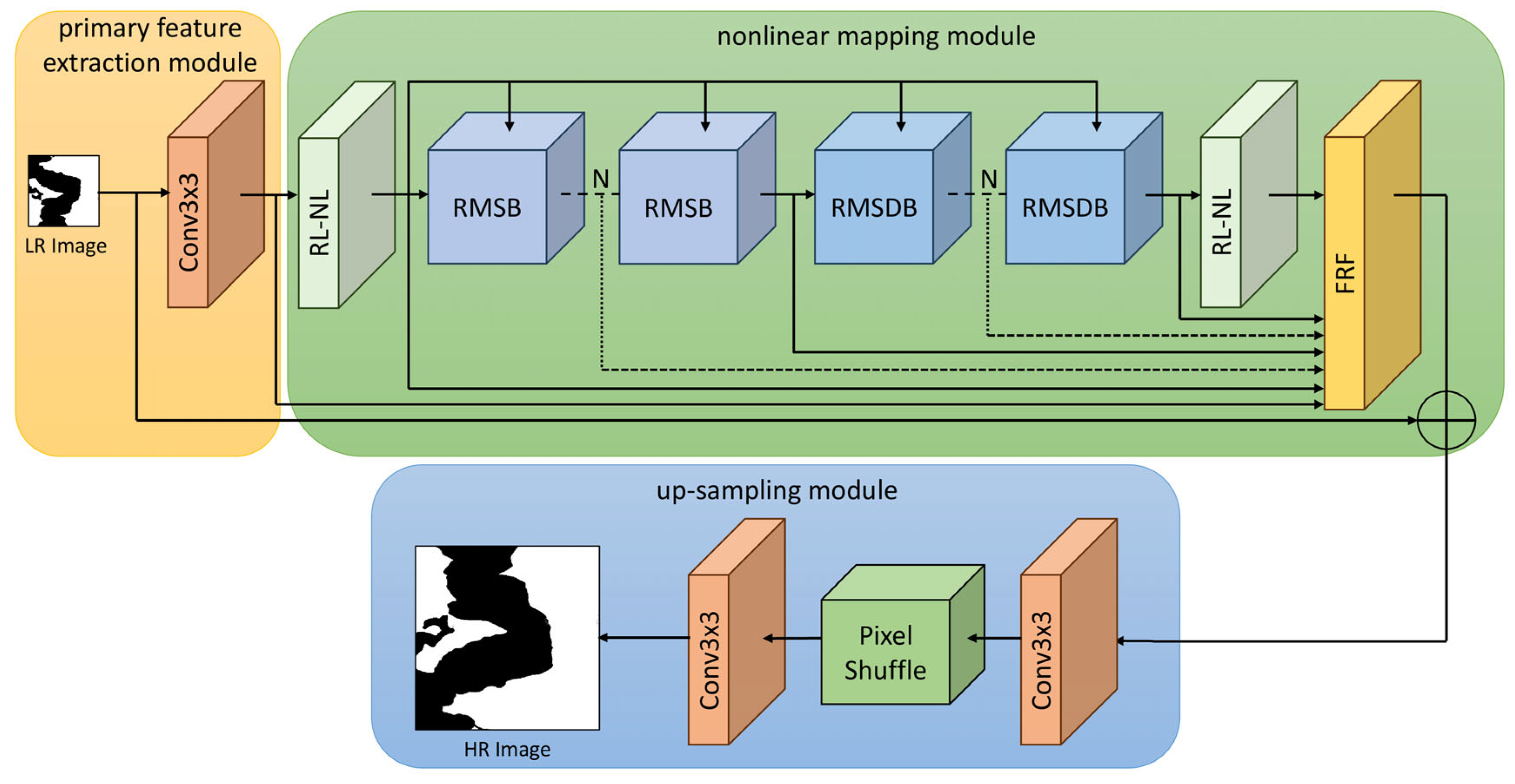
The proposed DEM-AMSSRN is an adaptation of the asymmetric multi-scale SR network (AMSSRN) optimized for DEM data. It is designed to upsample low-resolution elevation inputs while preserving fine topographic details and overall structural integrity [25]. As demonstrated in Figure 2, DEM-AMSSRN comprises three main components: (1) a primary feature extraction module (yellow) that processes the input DEM; (2) an advanced nonlinear mapping module (green) that includes two RL-NL modules [26] to capture long-range spatial dependencies, followed by residual multi-scale blocks (RMSBs) and residual multi-scale dilation blocks (RMSDBs) for hierarchical feature extraction, and (3) a precision upsampling module (blue) that produces the high-resolution output via two 3 × 3 convolutional layers with a sub-pixel convolution layer (PixelShuffle) [27] for high-quality output generation. A novel feature propagation mechanism feeds the output of the first RL-NL module into both the RMSB and RMSDB streams, and a feature refinement fusion (FRF) module intelligently combines shallow and deep features. Together, these innovations substantially improve reconstruction accuracy and stability. In our experiments, DEM-AMSSRN achieved notable gains in perceptual quality and even downstream terrain analysis accuracy, outperforming state-of-the-art alternatives.

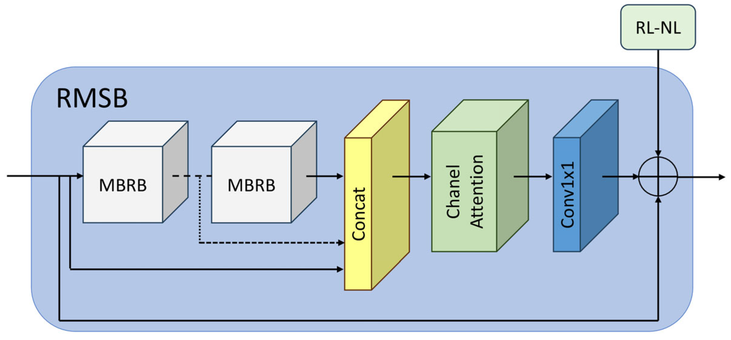
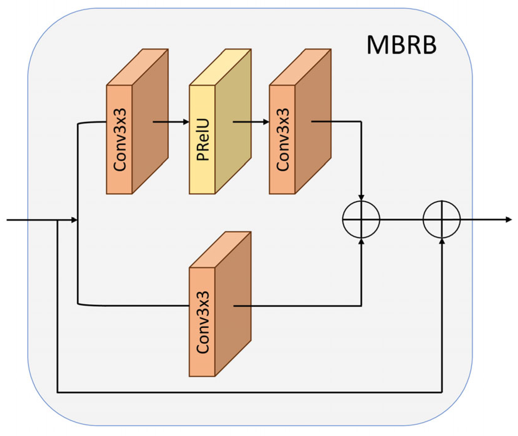
The RMSB (residual multi-scale block), depicted in Figure 3, has a parallel multi-branch design consisting of multiple MBRBs (multi-branch residual blocks), with each MBRB’s detailed structure illustrated in Figure 4. Each MBRB processes input features along two paths: an upper path with dual 3 × 3 convolutional layers for hierarchical feature extraction, and a lower path with a single 3 × 3 convolution for efficient local feature capture. The outputs of these two paths are merged and added back to the input (residual connection) to preserve low-level information. To maximize feature utilization, all MBRB outputs are concatenated and processed through a channel attention mechanism, which reweights channels to emphasize important features and suppress less informative ones. Finally, a 1 × 1 convolutional layer condenses the feature maps, and another residual connection adds the initial RMSB input to the output. This architecture allows each RMSB to capture multi-scale features and adaptively highlight critical information.

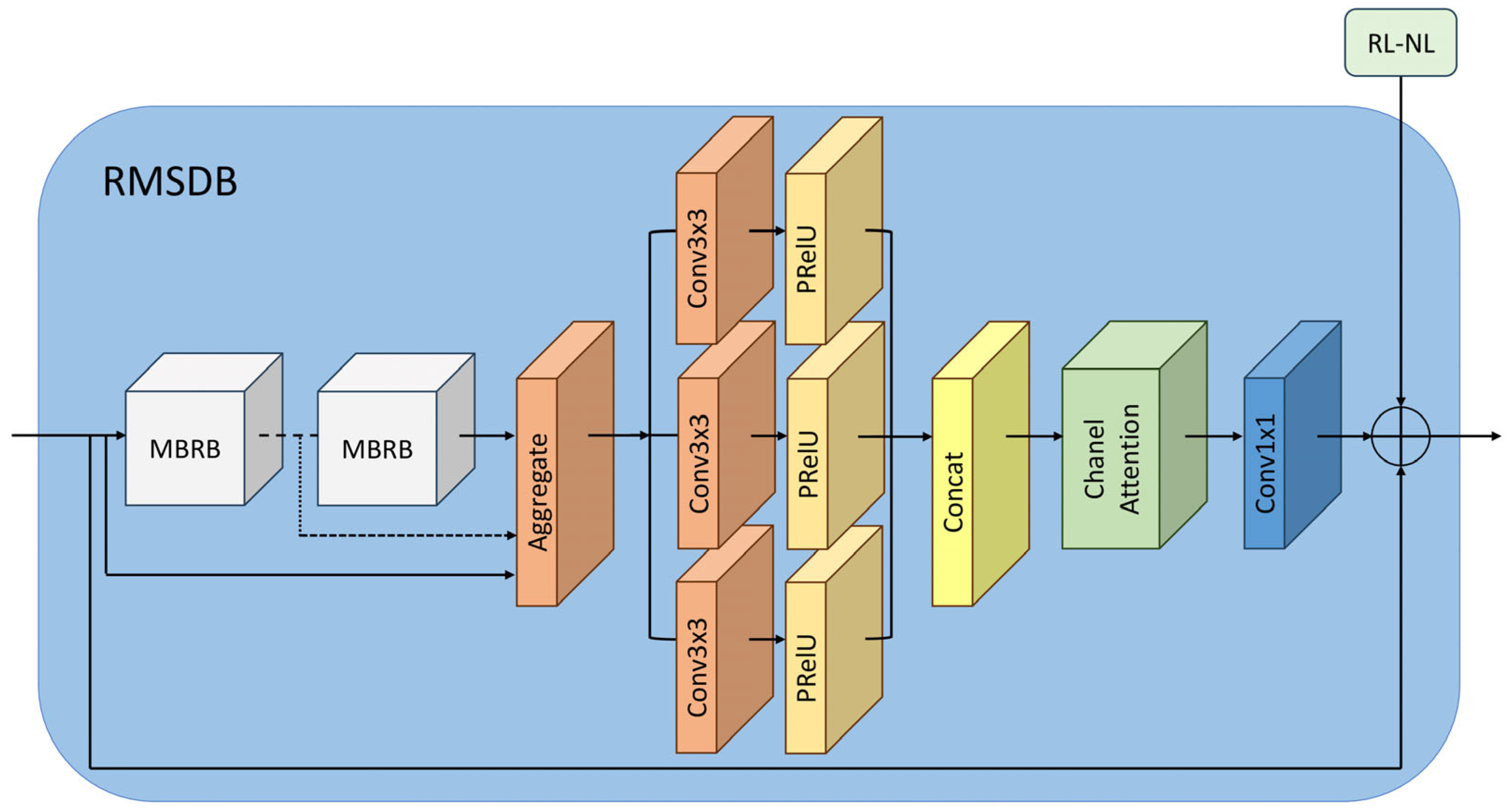
The RMSDB, illustrated in Figure 5, extends an RMSB by incorporating dilated convolutions to further increase the receptive field. In an RMSDB, multiple MBRBs are stacked, and a parallel branch applies dilated convolutions with various dilation rates. After aggregating features from all MBRBs, the combined output passes through the dilated convolution branch and is subsequently refined via the channel attention (CA) mechanism [28], which adaptively emphasizes semantically informative channels. A 1 × 1 convolution is then applied for dimensionality reduction, and the result is fused with the module’s original input through a residual connection to generate the intermediate RMSDB output.

To ensure cross-level feature consistency, a hierarchical refinement strategy is employed. Specifically, the output of the current module $O_x$ is fused with the output from the subsequent level $O_{x+1}$ via a convolutional operation. The fusion process is expressed as follows:

$$O_X^{\prime }=f\left(O_x+O_{x+1}\right)$$

(2)

The upsampling module utilizes an advanced PixelShuffle operation (illustrated in Figure 6) to achieve high-quality resolution enhancement through an intelligent channel-to-space transformation. This sophisticated technique fundamentally reorganizes multi-channel feature information into expanded spatial dimensions while preserving critical topographic relationships in the elevation data.

Mathematically, the operation transforms an input tensor $X\in R^{b,c\times r^2,h,w}$ into a higher-resolution output $Y\in R^{^b,c,h\times r,w\times r}$ through a periodic rearrangement of channel elements. Here, b denotes the batch size, c the number of output channels, h and w the spatial dimensions of the input feature map, and r is the integer upscaling factor. PixelShuffle rearranges a multi-channel tensor into a higher-resolution output by redistributing channel values into expanded spatial positions. This learnable upsampling method preserves all the original feature information and, when preceded by appropriate convolutions, avoids the “checkerboard” artifacts often caused by naive transpose-convolution upsampling. As a result, fine-grained elevation gradients are maintained and topographic continuity is preserved in the super-resolved output.

2.4. Loss Function

The proposed framework employs a composite loss function integrating pixel-wise, perceptual, and adversarial components to holistically optimize super-resolution performance.

The pixel loss component utilizes the $L_1$ norm to measure absolute differences between generated and ground truth images, providing enhanced edge preservation and robustness to outliers compared to the $L_2$ norm, while ensuring faithful reconstruction of low-frequency structural elements. For perceptual optimization, a 19-layer visual geometry group (VGG) network extracts high-level features, with loss computed as the Euclidean distance between deep feature representations:

$$L_{perceptual}(I_{SR},I_{HR},\mathit{\varphi },l)=\left|{\mathit{\varphi }}_l(I_{SR}-I_{HR})\right|$$

(3)

where ${\varphi }_l(·)$ denotes activations from the $l$-th layer of the pre-trained VGG network. This component effectively captures textural and semantic information that pixel-level metrics may miss.

The adversarial loss, implemented via relativistic discriminator principles [29], enhances visual realism through min–max optimization:

$$L_{adversarial}(I_{SR},I_{HR})={\rm E}\left(D\right(I_{HR})-{\rm E}(D\left(I_{SR}\right)\left)\right)-{\rm E}\left(D\right(I_{SR})-{\rm E}(D\left(I_{HR}\right)\left)\right)$$

(4)

where $I_{SR}$ denotes the super-resolved (generated) image, $I_{HR}$ is the corresponding high-resolution (ground truth) image, $D(·)$ represents the discriminator network’s output, ${\rm E}(·)$ denotes the expectation operation. The first term ${\rm E}\left(D\right(I_{HR})-{\rm E}(D\left(I_{SR}\right)\left)\right)$ encourages the discriminator to distinguish real images. The second term ${\rm E}\left(D\right(I_{SR})-{\rm E}(D\left(I_{HR}\right)\left)\right)$ promotes the generator to fool the discriminator. The relativistic formulation compares the discriminator’s responses to real and generated images in both directions.

Finally, the total loss function is formulated as follows:

$$Los{s}_G=\alpha L_{pixel}+\beta L_{perceptual}+\gamma L_{adversarial}$$

(5)

where $\alpha$, $\beta$, and $\gamma$ represent carefully balanced weighting coefficients.

2.5. Model Training Optimization Strategy

We trained DEM-AMSSRN and several baseline models for comparison. The baseline deep SR models include SRGAN [30], SRAGAN (a sparsity and attention-based GAN) [31], NDSRGAN (a dense GAN for aerial images) [32], and SRADSGAN (the D-SRCAGAN method with dense-sampling and residual attention) [33], all adapted to our DEM data. These models were chosen because they represent widely used GAN-based SR architectures with progressively enhanced mechanisms: SRGAN as the classical GAN-based SR framework, SRAGAN introducing sparsity and attention, NDSRGAN designed for dense aerial imagery, and SRADSGAN integrating dense sampling with residual attention. By adapting them to DEM data, we ensured a fair comparison against state-of-the-art approaches that emphasize different design strategies relevant to high-resolution surface reconstruction. We re-trained each model on our dataset, modifying only the input/output channels (to single-channel DEM data) and any obvious architecture tweaks needed to handle elevation data (e.g., removing batch-norm layers if they hindered training stability). All GAN-based models were trained using the WGAN-GP approach [34], which replaces the classic GAN’s binary cross-entropy loss with a Wasserstein loss and adds a gradient penalty term for improved stability. This approach replaces the original WGAN’s problematic weight clipping [35] with a gradient penalty term that directly enforces the 1-Lipschitz condition through regularization of the discriminator’s gradients on interpolated samples.

This modification yields three key benefits: it (1) mitigates vanishing gradient issues, (2) alleviates mode collapse, and (3) maintains the discriminator’s critic capacity at an optimal level throughout training. Furthermore, we implemented an adaptive learning rate adjustment mechanism that monitors validation MSE trends: a sequence of degradations triggers successive 10% reductions in both generator and discriminator learning rates (initial values: $1\times {10}^{-5}$ for the generator and $1\times {10}^{-5}$ for the discriminator). This adaptive strategy, combined with spectral normalization across all discriminator layers, promotes stable convergence and mitigates entrapment in local optima, which is particularly critical for DEM reconstruction, where elevation accuracy is paramount. The complete training protocol employs Adam optimization (b1 = 0.9, b2 = 0.999) with mini-batch processing (size = 16) over 300 epochs, striking an optimal balance between reconstruction fidelity and computational efficiency.

3. Experiment and Results

3.1. Experimental Setup

Our experiments were carried out in a consistent environment and with reproducible settings.

Table 3. Experimental environment and key parameters.

Environment	Version
Computer System	Ubuntu 20.04.1
PyTorch	1.8.1
CPU	Intel(R) Xeon(R) Silver 4310 CPU @ 2.10 GHz
GPU	GeForce RTX 4090 (24 G × 2)
Batch size	64
G_Learning Rate	$1\times {10}^{-5}$
D_Learning Rate	$1\times {10}^{-5}$
b1	0.9
b2	0.999
Optimizer	Adam
α	100
β	1
γ	0.1

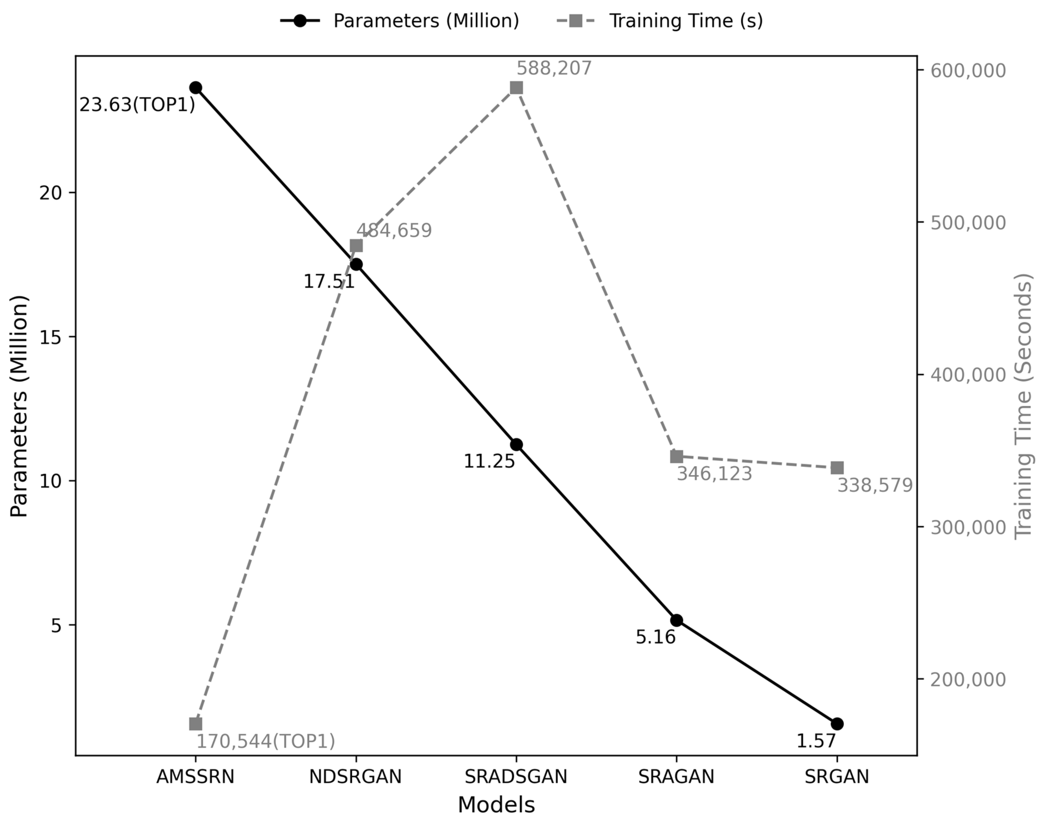
summarizes the hardware (CPU, GPUs), software (OS, library versions), and key training parameters for transparency. We evaluated five deep learning SR models (the four baselines mentioned and our DEM-AMSSRN) in terms of both accuracy and computational requirements. Figure 7 compares the models’ training times and number of parameters, illustrating the trade-offs between model complexity and speed. In terms of parameter scale and training efficiency, AMSSRN demonstrates a clear advantage over the GAN-based counterparts. Specifically, AMSSRN contains 23.63 M parameters, which is larger than SRGAN (1.57 M) and SRAGAN (5.16 M) but remains within a reasonable range compared with NDSRGAN (17.51 M) and SRADSGAN (11.25 M). More importantly, AMSSRN requires only 170,544 s for training, which is significantly shorter than NDSRGAN (484,659 s), SRADSGAN (588,207 s), SRAGAN (346,123 s), and SRGAN (338,579 s). This indicates that AMSSRN achieves a favorable balance between model complexity and training efficiency. The key reason behind this improvement is that AMSSRN adopts a CNN-based architecture, while all other compared methods are GAN-based models. The GAN-based frameworks generally involve adversarial training with both generator and discriminator, which introduces additional computational overhead and instability, leading to substantially longer training times. Therefore, AMSSRN not only reduces training cost but also provides a more practical solution for large-scale, high-resolution applications.

3.2. Evaluation Metrics

We used three standard metrics to quantitatively evaluate super-resolution performance:

RMSE (root mean square error): This measures the average reconstruction error in elevation. Lower RMSE indicates higher accuracy. For each test case, RMSE is computed in meters. The RMSE is defined as follows:

$$RMSE=\sqrt{{\displaystyle \frac{1}{N}}\sum _{i=1}^N(x_i-{\hat{x}}_i{)}^2}$$

(6)

where, $x_i$ is the value of the original DEM, $\widehat{x_i}$ is the value of the super-resolution DEM, and N is the number of sampling points.

PSNR (peak signal-to-noise ratio): This metric (in dB) is derived from the mean squared error (MSE) between the super-resolved DEM and the ground truth. Higher PSNR indicates that the reconstructed DEM is closer to the ground truth in terms of overall intensity. To compute PSNR, the mean squared error (MSE) is first calculated, which is also commonly used as a loss function in optimization tasks. The MSE is defined as follows:

$$MSE={\displaystyle \frac{1}{N}}\sum _{i=1}^N(x_i-{\hat{x}}_i{)}^2$$

(7)

The PSNR is then calculated as follows:

$$PSNR=10{\mathit{log}}_{10}\left({\displaystyle \frac{L^2}{MSE}}\right)$$

(8)

here, L represents the maximum possible pixel value. For 8-bit images, L is typically 255. However, since DEMs often contain grayscale values much larger than 255, L is adjusted to the difference between the maximum and minimum grayscale values in the DEM dataset to better reflect the dynamic range.

SSIM (structural similarity index): This metric evaluates image similarity in terms of structure, luminance, and contrast. SSIM ranges from 0 to 1, with 1 meaning perfect structural identity with the ground truth. It is sensitive to the preservation of spatial patterns and textures. Because SSIM alone may not capture all types of error (it can be high even if absolute errors exist, as long as structural patterns are similar), we consider it alongside RMSE and PSNR for a comprehensive assessment. The SSIM formula is defined as follows:

$$SSIM(x,y)={\displaystyle \frac{(2{\mu }_x{\mu }_y+c_1)(2{\sigma }_{xy}+c_2)}{({\mu }_x^2+{\mu }_y^2+c_1)({\sigma }_x^2+{\sigma }_y^2+c_2)}}$$

(9)

where, ${\mu }_x$ and ${\mu }_y$ denote the mean intensities of images x and y; ${\sigma }_x$ and ${\sigma }_y$ represent their variances; and ${\sigma }_{xy}$ is the covariance between the two images. The constants $c_1$ and $c_2$ are included to prevent division by zero.

All metrics are computed on the test set for each model. In the tables below, we boldface the best (most favorable) values for each metric.

3.3. Pixel Metrics Results of SR for the U.S. Coastal DEM Dataset

We evaluated DEM-AMSSRN against the baseline methods on ten representative test regions (denoted TEST1 through TEST10) from the U.S. coastal DEM dataset. The elevation statistics of these regions, including minimum, maximum, mean, median, and standard deviation, are summarized in

Table 4. Elevation statistics for the 10 TEST regions (meters).

TASK	MIN	MAX	MEAN	MIDDLE	STD
TEST1	−13.8496	14.4189	−3.1874	−1.6619	3.3270
TEST2	−202.6674	8.7705	−50.4739	−12.0973	58.5573
TEST3	6.2794	26.5965	13.9677	13.5799	2.5370
TEST4	−24.1892	9.0238	−13.3086	−14.6355	6.3288
TEST5	−18.3500	21.6559	−1.1026	1.7662	10.1626
TEST6	−11.2520	13.4902	0.9356	0.6129	3.5818
TEST7	−10.9666	68.0736	27.3460	27.1557	9.9206
TEST8	−5.6956	153.9967	55.4630	53.3872	21.4533
TEST9	−6.8167	239.3325	93.5620	88.2389	31.9134
TEST10	−244.6157	169.2753	−0.0399	44.3003	120.6732

.

Table 5. RMSE of reconstructed DEMs (in meters) for 10 test cases (scale 3×). Bold values indicate the best performance within each test.

TASK	Bicubic	DEM-AMSSRN	SRGAN	SRAGAN	NDSRGAN	SRADSGAN
TEST1	0.00254	0.00251	0.00272	0.00290	0.00254	0.00255
TEST2	0.00248	0.00192	0.00424	0.00451	0.00190	0.00429
TEST3	0.01456	0.01143	0.01182	0.01206	0.01157	0.01159
TEST4	0.00053	0.00044	0.00053	0.00049	0.00043	0.00044
TEST5	0.00805	0.00629	0.00653	0.00665	0.00635	0.00635
TEST6	0.00778	0.00625	0.00645	0.00659	0.00632	0.00630
TEST7	0.00815	0.00316	0.00338	0.00372	0.00331	0.00328
TEST8	0.04366	0.02875	0.02972	0.03052	0.02896	0.02896
TEST9	0.04038	0.02566	0.02653	0.02754	0.02576	0.02581
TEST10	0.06550	0.03206	0.33849	0.30909	0.03263	0.06343
MEAN	0.01936	0.01185	0.04304	0.04041	0.011980	0.01530

reports the RMSE for each method on each test, as well as the mean RMSE across all tests. Our DEM-AMSSRN exhibits the lowest reconstruction error in all cases, with a mean RMSE of 0.01185. This is less than half the error of bicubic interpolation (mean RMSE 0.02541) and also lower than the errors of the GAN-based models. In challenging regions with complex terrain (e.g., TEST3, TEST5, and TEST10 in Table 4), conventional models have higher errors, whereas DEM-AMSSRN maintains low errors—for example, in TEST10 (an urban coastal area with varied elevation), our RMSE is 0.03206, compared to 0.06343 with SRADSGAN and ~0.06550 with bicubic. In percentage terms, DEM-AMSSRN reduces RMSE by ~38.7–62.3% relative to the next-best model (often NDSRGAN) on these difficult tests. This indicates a significantly improved capacity to recover fine terrain details.

In terms of signal fidelity,

Table 6. PSNR (dB) for 10 test cases (scale 3×). Bold values indicate the best performance within each test.

TASK	Bicubic	DEM-AMSSRN	SRGAN	SRAGAN	NDSRGAN	SRADSGAN
TEST1	49.13	49.19	48.83	48.55	49.14	49.12
TEST2	44.92	46.04	42.58	42.32	46.07	42.54
TEST3	46.87	47.92	47.77	47.68	47.86	47.86
TEST4	51.86	52.68	51.87	52.17	52.74	52.73
TEST5	47.65	48.72	48.56	48.49	48.69	48.68
TEST6	43.69	44.64	44.50	44.41	44.59	44.61
TEST7	57.55	61.67	61.37	60.96	61.46	61.50
TEST8	57.35	59.16	59.02	58.90	59.13	59.13
TEST9	61.52	63.49	63.34	63.18	63.47	63.46
TEST10	56.41	59.51	49.28	49.67	59.44	56.55
MEAN	51.67	53.30	51.71	51.63	53.26	52.62

shows the PSNR results. DEM-AMSSRN achieves an average PSNR of 53.30 dB, which is the highest among all methods (for reference, bicubic averages 51.67 dB). This ~1.6 dB gain over bicubic and ~1.2 dB over the next-best model (NDSRGAN at 52.62 dB) is significant given that PSNR is on a logarithmic scale. Notably, in test regions with relatively large errors (e.g., TEST8 and TEST9 where bicubic PSNRs are ~57 dB and ~61.5 dB), DEM-AMSSRN pushes PSNR to ~59–63 dB, indicating better overall reconstruction quality. Such improvements are crucial for elevation data; even small error reductions (reflected in a couple of dB PSNR) can materially impact applications like flood modeling, where errors might accumulate or threshold effects might be triggered.

Lastly,

Table 7. SSIM for 10 test cases (scale 3×). Bold values indicate the best performance within each test.

TASK	Bicubic	DEM-AMSSRN	SRGAN	SRAGAN	NDSRGAN	SRADSGAN
TEST1	0.994700	0.994664	0.994156	0.993700	0.994627	0.994651
TEST2	0.989464	0.990351	0.983332	0.977483	0.990454	0.984945
TEST3	0.994563	0.995319	0.995063	0.994828	0.995286	0.995295
TEST4	0.996962	0.997325	0.997173	0.996980	0.997361	0.997339
TEST5	0.989357	0.991034	0.990697	0.990469	0.990958	0.990972
TEST6	0.981308	0.984390	0.983670	0.983323	0.984290	0.984063
TEST7	0.999390	0.999568	0.999529	0.999459	0.999557	0.999555
TEST8	0.998837	0.999011	0.998976	0.998936	0.999008	0.999006
TEST9	0.999555	0.999621	0.999608	0.999590	0.999623	0.999622
TEST10	0.999083	0.999272	0.999033	0.998658	0.999268	0.999016
MEAN	0.994322	0.995056	0.994124	0.993343	0.995043	0.994446

lists the SSIM results. All deep learning models achieve very high SSIM (≥0.993 on average), reflecting that they all preserve the overall structural layout of the terrain quite well (much better than bicubic’s mean SSIM 0.9943, which is already high because bicubic does not severely distort structures; it just blurs them). DEM-AMSSRN attains the highest mean SSIM, 0.995056, indicating near-perfect structural similarity to the ground truth. The differences among the models are subtle but telling: for instance, in TEST7 (which includes man-made structures and natural terrain), DEM-AMSSRN reaches SSIM 0.999568, whereas the next best (NDSRGAN) is 0.999557—a small numerical difference, but it consistently appears across tests, especially those with sharp features. In the coastal transition zone of TEST3, our method’s SSIM is 0.995319 vs. 0.995286 (NDSRGAN) and ~0.99456 (bicubic). These slight improvements indicate that DEM-AMSSRN better preserves fine structural details, like the continuity of a shoreline or the texture of an urban coastline, which are slightly blurred or distorted by other models. Traditional GAN baselines, such as SRGAN and SRAGAN, show more pronounced drops in SSIM in certain tests (e.g., SRAGAN is 0.998658 in TEST10 vs. our 0.999272), which correspond to instances where those models introduced artifacts that break structural consistency.

In summary, across all metrics, DEM-AMSSRN demonstrates superior performance. The combination of low RMSE, high PSNR, and near-perfect SSIM suggests that our model not only predicts the correct elevation values on average but also preserves the overall visual and structural quality of the terrain better than prior methods. This is crucial in practice: for instance, even if two models have similar RMSE, the one with higher SSIM will yield outputs more useful for visual analysis or further modeling (because the terrain features appear visually accurate). Our results indicate that DEM-AMSSRN provides a more faithful super-resolution of coastal DEMs, improving both quantitative accuracy and qualitative realism.

3.4. Visual Quality of SR for the U.S. Coastal DEM Dataset

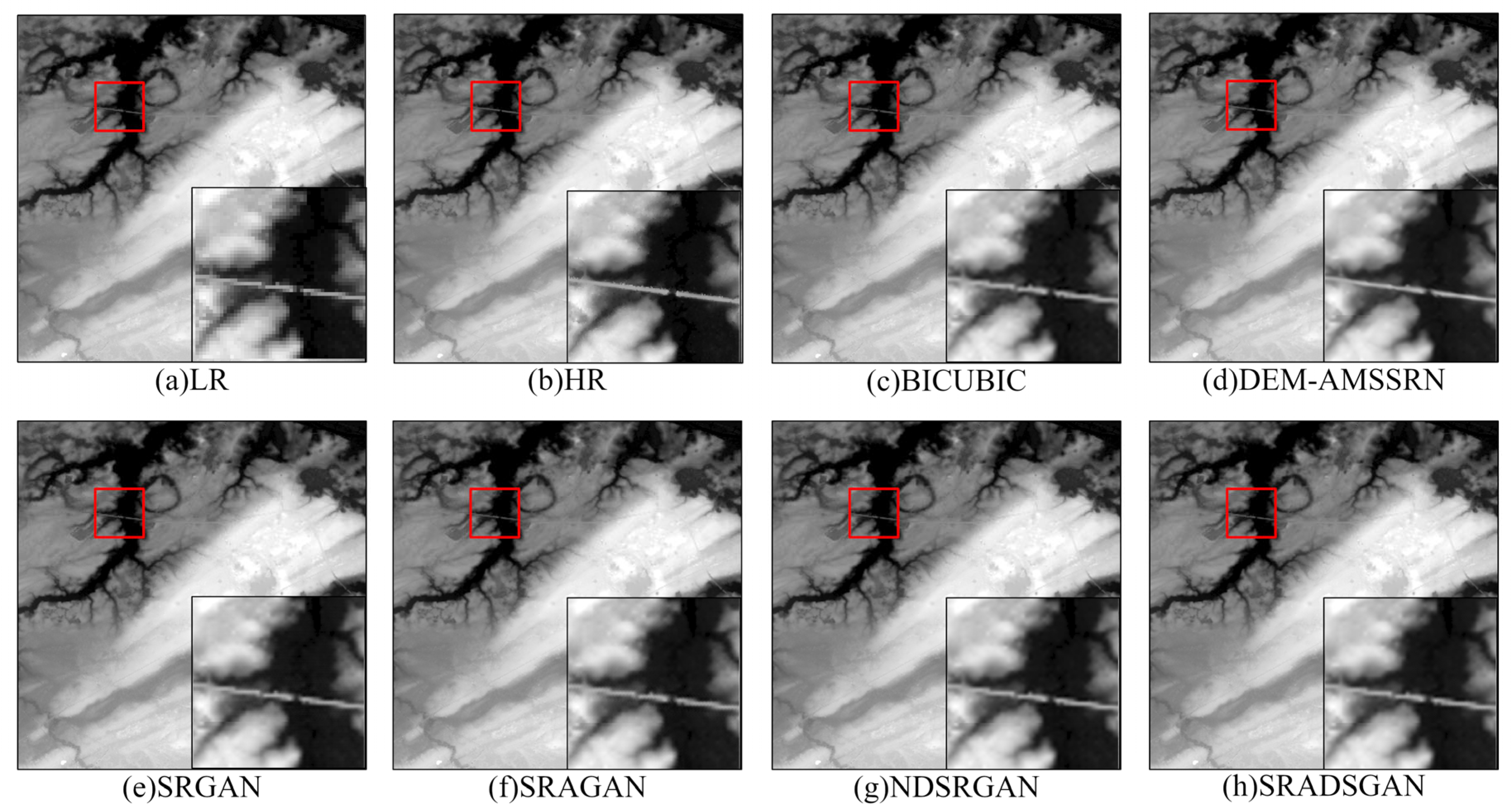
While numerical metrics are important, visual inspection provides intuitive insight into model performance. We therefore compare the super-resolved DEM outputs qualitatively for representative regions. Figure 8 shows a comparison of TEST5 results ((a) coastal area with a mix of natural and urban features). The bicubic interpolation result (Figure 8c) is visibly smoother and lacks fine detail compared to the ground truth (Figure 8b). It blurs small creek channels and softens building edges. The four baseline DL models (Figure 8e–h) recover some details: e.g., SRGAN (Figure 8e) sharpens edges slightly but introduces some checkerboard noise; SRAGAN (Figure 8f) preserves a few linear features with its attention mechanism but still misses smaller textures; NDSRGAN (Figure 8g) produces generally good detail but some structures are misplaced slightly; SRADSGAN (Figure 8h) does well in flatter areas but oversmooths some high-frequency content (likely due to its residual filtering approach). In contrast, DEM-AMSSRN (Figure 8d) produces an output closest to the ground truth: the coastline and sandbar features are crisp, small tributary patterns are clearly delineated, and urban structures (bright spots) are more distinct and correctly shaped, with fewer artifacts. The zoomed insets highlight that DEM-AMSSRN maintains continuous ridgelines and shoreline contours that other models break or blur.

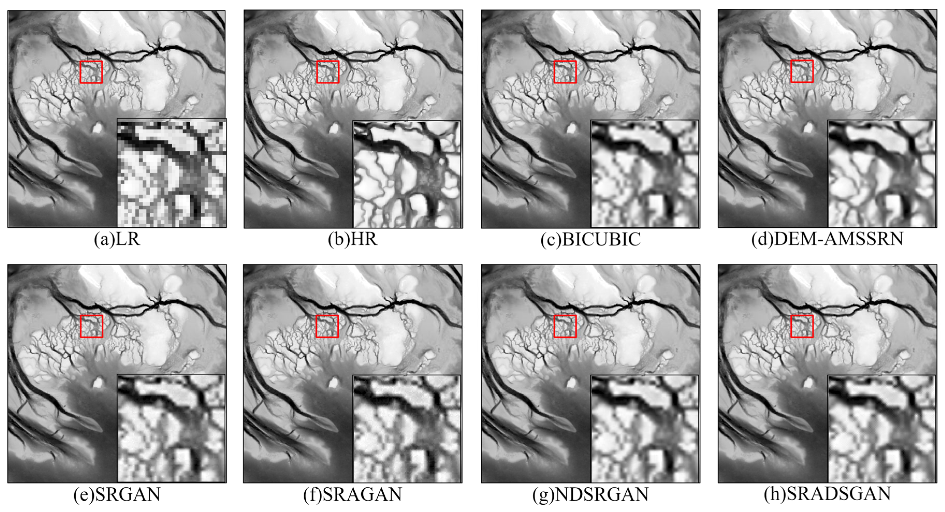
Another example, Figure 9, focuses on TEST7, which includes complex geomorphology (tidal channels, mudflats) and human-made structures (levees, roads). Bicubic (Figure 9c) fails to recover the narrow tidal channels and simply blurs them into the surroundings. SRGAN (Figure 9e) and SRAGAN (Figure 9f) start to recover some channel structure but generate rippling artifacts and slightly jagged edges. NDSRGAN (Figure 9g) improves the channel clarity but seems to over-enhance some noise as well (some grid-like artifacts are visible, possibly from its dense sampling strategy). SRADSGAN (Figure 9h) produces relatively smooth results but at the cost of losing some fine channel intricacy. DEM-AMSSRN (Figure 9d), however, manages to clearly reconstruct the network of tidal channels with smooth, continuous curves and correct widths. The levee embankments in the scene are also better defined, illustrated as straight lines in DEM-AMSSRN’s output, whereas other models exhibit waviness. The error maps (Figure 10, next) corroborate these observations quantitatively: DEM-AMSSRN’s errors are low and uniformly distributed, whereas other models have concentrated errors along these critical features (indicating either under- or overshooting the elevations there).

To further illustrate model performance, Figure 10 presents error maps for TEST8. Red corresponds to low errors, whereas blue denotes high errors. The bicubic error map contains extensive blue regions, reflecting large deviations—an expected outcome given its inability to reconstruct fine details. In contrast, the deep learning models substantially reduce errors, with more areas shifting toward green, yellow, and red. However, SRGAN and SRAGAN exhibit localized dark-blue patches, corresponding to severely mispredicted features such as flattened small hills or artificially introduced bumps. NDSRGAN and SRADSGAN yield fewer extreme errors but still display a mottled distribution of alternating positive and negative error speckles, likely caused by residual high-frequency noise. By comparison, DEM-AMSSRN produces error maps that are predominantly red and yellow, indicating not only small error magnitudes but also smoothly varying residuals, without pronounced localized spikes. This suggests that our model achieves consistently low errors while avoiding structured artifacts that would otherwise manifest as patterned errors.

In summary, the visual comparisons confirm the quantitative results: DEM-AMSSRN reconstructs DEM details with higher fidelity, maintaining both the overall terrain structure and the fine features such as channels, ridges, and man-made structures better than previous methods. It produces sharper and more realistic elevation patterns, with fewer artifacts. This is crucial for end-use: a super-resolved DEM that appears visually accurate will be more reliable for any subsequent analysis (flood simulations, terrain analysis, etc.) than one with unnatural discontinuities or blurred features.

3.5. Construction of the U.S. 1/9 Arc-Second Offshore DEM

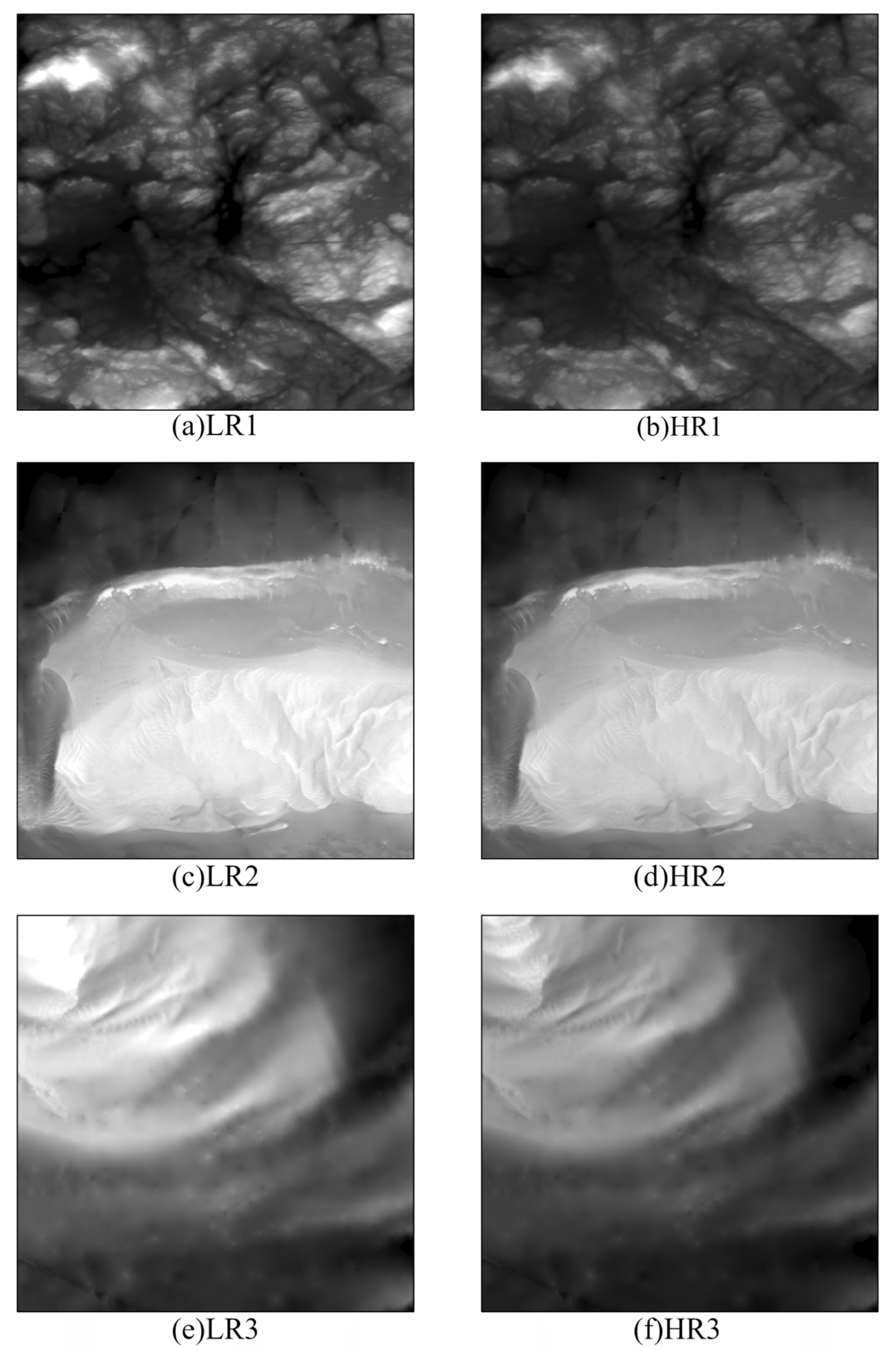
Using DEM-AMSSRN, we generated the USA_OD_2025 dataset, the first comprehensive 1/9 arc-second (~3 m) offshore DEM covering the major U.S. coastal regions. Our input was the CUDEM 1/3 arc-second DEM (CONUS: NAVD88), which provides 10 m resolution data for U.S. coasts. We applied our trained model to enhance this data by a factor of 3× in resolution. The result is USA_OD_2025, a seamless high-resolution DEM dataset for U.S. coastlines, including the East Coast, West Coast, Gulf Coast, and Alaska (where source data were available).

USA_OD_2025 represents a threefold enhancement in resolution over previously available offshore DEM products. This enables the detection of bathymetric and topographic features at the sub-10 m scale, which were not resolvable in the 1/3″ (~10 m) data. For example, small sandbar formations, narrow tidal creeks, and fine harbor structures that were blurred in the original data can now be distinguished. Figure 11 provides visual comparisons in three regions: in each case, the 1/9″ DEM (right sub-figure) reveals sharper and more detailed features than the 1/3″ DEM (left sub-figure). In panel (a) vs. (b), offshore sand wave patterns that are only vaguely hinted at in the 10 m DEM become clear undulating forms in the 3 m DEM. In (c) vs. (d), a coastal city’s waterfront shows piers and breakwaters in the high-res DEM that are absent in the low-res. In (e) vs. (f), intricate channel networks in a delta or marsh area are significantly better resolved.

Beyond the qualitative improvements, USA_OD_2025 is anticipated to exert significant scientific and practical impacts. Scientifically, the availability of a ~3 m resolution DEM along the entire U.S. coast enables new investigations into fine-scale coastal and marine processes—such as sediment transport dynamics around tidal inlets, detailed benthic habitat mapping, and small-scale morphological changes induced by storms—that were not feasible with coarser-resolution products. Practically, numerous engineering and management applications stand to benefit: storm surge and tsunami models can exploit the finer DEM to improve local inundation predictions; coastal infrastructure projects, such as the design of seawalls and navigational channels, can rely on more accurate seabed topography; and conservation initiatives, including wetland restoration, can better assess terrain–ecosystem interactions.

In generating USA_OD_2025, care was taken to minimize artifacts introduced by the super-resolution process. Validation against higher-resolution reference data (e.g., LiDAR surveys and sounding measurements) demonstrated good agreement, with errors typically within the nominal 0.76 m RMSE of the source dataset. Seamlines between adjacent tiles were also smoothed to ensure a seamless product.

In conclusion, USA_OD_2025, produced by our DEM-AMSSRN model, is a transformative dataset for the U.S. coastal community, providing a level of detail previously inaccessible at the national scale. We release this dataset openly to encourage further research and development in coastal science, hazard mitigation, and marine spatial planning.

4. Discussions

The proposed DEM-AMSSRN framework addresses the critical challenge of preserving both large-scale geomorphological structures and fine-scale topographic details in offshore DEM reconstruction. By integrating RL-NL for long-range spatial dependency modeling and RMSB for hierarchical feature extraction, our approach effectively captures continental shelf-scale bathymetric trends alongside localized terrain textures. The hybrid loss function further enhances geometric fidelity and visual realism, enabling superior reconstruction performance compared to existing methods.

Experimental results on U.S. offshore DEM datasets demonstrate the model’s significant advantages over GAN-based approaches, achieving a 72.47% reduction in RMSE (vs. SRGAN) and exceptional quantitative metrics (53.30 dB PSNR, 0.995056 SSIM). These improvements validate the framework’s capability to support high-precision applications in coastal geomorphology analysis, marine resource management, and disaster prevention. To facilitate further research, we release USA_OD_2025, a novel high-resolution (1/9 arc-second) offshore DEM dataset covering major U.S. coastal zones, serving as both a benchmark and a resource for future studies.

One limitation to note is that while our model improves resolution to ~3 m, it does not add new ground truth information beyond what was inferable from the coarse input. Extremely fine features that were completely absent in the input (e.g., a very narrow pier that is smaller than the input resolution) cannot be perfectly reconstructed. In such cases, DEM-AMSSRN will produce a plausible guess (often a smoothed or slightly hallucinated feature), which might not correspond to reality. This is a known limitation of super-resolution models—they cannot invent detail with full certainty. We mitigated this by training on real high-res DEM patches, so the model’s “hallucinations” are statistically likely to resemble real features, but users of the USA_OD_2025 dataset should be aware that the finest details, especially if they look like isolated small structures, should be used with caution (or cross-validated with imagery or LiDAR if possible).

We also observed that our model, like many deep networks, can be sensitive to input data that lie outside the distribution seen during training. If, for example, a region of the U.S. coastline has a very different morphology than anything in our 60 training tiles (though we tried to capture all major types), the reconstruction quality might degrade. This has not been a serious issue in our tests—the model handled all U.S. coastal types well—but it suggests that generalizing to non-U.S. coastlines might require some fine-tuning or transfer learning, especially in areas with fundamentally different geomorphology or anthropogenic features.

Several promising research directions stem from this work:

• Architectural improvements: Newer network architectures, such as vision transformers or diffusion models, could be explored for DEM super-resolution. These have shown remarkable results in image synthesis and could capture even more global context than our RL-NL modules. However, they come with increased computational cost, so a trade-off analysis would be needed.
• Multimodal data fusion: Reconstruction fidelity could be improved by integrating complementary data modalities (e.g., LiDAR point clouds, multispectral satellite imagery, multibeam sonar bathymetry). Such approaches would be particularly valuable for dynamic coastal interfaces and ecologically sensitive wetlands, where terrain complexity challenges single-modality methods.
• Uncertainty quantification: It would be valuable to quantify the uncertainty of the super-resolved DEM. Techniques like Monte Carlo dropout or training an ensemble of models could provide pixel-wise uncertainty estimates. This is especially relevant for decision-makers using the data; knowing which areas of the DEM are less certain (perhaps due to a lack of similar training examples) can guide ground-truth data collection or cautious interpretation.

5. Conclusions

We presented DEM-AMSSRN, an asymmetric multi-scale super-resolution network for offshore DEM enhancement. DEM-AMSSRN effectively balances the preservation of large-scale geomorphological structures with the reconstruction of fine-scale topographic details. Leveraging region-level non-local modules and residual multi-scale blocks, the model captures both global context and local texture, achieving state-of-the-art performance, as evidenced by substantial improvements in RMSE, PSNR, and SSIM over existing approaches.

Utilizing this model, we generated USA_OD_2025, a 1/9 arc-second (~3 m) high-resolution offshore DEM dataset for U.S. coastal regions. This dataset provides a new level of detail for coastal topography, supporting advanced analysis in coastal geomorphology, marine resource management, and hazard modeling.

In future work, we envision integrating emerging deep learning techniques (e.g., transformers, physics-informed neural networks) and multi-source data to further improve DEM super-resolution. We also plan to extend our approach to other regions and possibly to 3D volumetric data (for subsurface models). By continuing to refine these techniques and datasets, we aim to contribute to more accurate and actionable coastal data, ultimately aiding in coastal resilience and sustainable ocean management.

References

- National Oceanic and Atmospheric Administration (NOAA). Population Trends Along the U.S. Coastline; NOAA National Ocean Service: Silver Spring, MD, USA, 2020. Available online: https://coast.noaa.gov/digitalcoast/training/population-report.html (accessed on 23 June 2025).
- National Oceanic and Atmospheric Administration (NOAA). Coastal Economy Data; NOAA Office for Coastal Management: Silver Spring, MD, USA, 2020. Available online: https://coast.noaa.gov/digitalcoast/data/coastaleconomy.html (accessed on 23 June 2025).
- Food and Agriculture Organization (FAO). The State of World Fisheries and Aquaculture 2022; FAO: Rome, Italy, 2022. [Google Scholar] [CrossRef]
- National Oceanic and Atmospheric Administration (NOAA). Technical Considerations for Use of Geospatial Data in Sea Level Change Mapping and Assessment; NOAA Coastal Services Center: Charleston, SC, USA, 2018. Available online: https://coast.noaa.gov/data/digitalcoast/pdf/slr-slc-tech.pdf (accessed on 23 June 2025).
- Dietrich, J.C.; Zijlema, M.; Westerink, J.J.; Holthuijsen, L.H.; Dawson, C.; Luettich, R.A.; Jensen, R.E.; Smith, J.M.; Stelling, G.S.; Stone, G.W. Modeling Hurricane Waves and Storm Surge Using Integrally-Coupled, Scalable Computations. Coast. Eng. 2011, 58, 45–65. [Google Scholar] [CrossRef]
- Grilli, S.T.; Harris, J.C.; Shi, F.; Kirby, J.T.; Tajalli Bakhsh, T. Numerical Modeling of Coastal Tsunami Inundation with GPU-Accelerated Boussinesq Wave Model. Nat. Hazards 2021, 106, 1299–1328. [Google Scholar] [CrossRef]
- Bevacqua, E.; Maraun, D.; Vousdoukas, M.I.; Voukouvalas, E.; Vrac, M.; Mentaschi, L.; Widmann, M. Higher Probability of Compound Flooding from Precipitation and Storm Surge in Europe Under Anthropogenic Climate Change. Sci. Adv. 2019, 5, eaaw5531. [Google Scholar] [CrossRef] [PubMed]
- Hajiesmaeeli, M.; Medrano, F.A.; Tissot, P. Generation of Offshore Area DEMs Using Oblique Stereo Imagery. In Proceedings of the I-GUIDE Forum 2024, West Lafayette, IN, USA, 15–17 May 2024; Available online: https://docs.lib.purdue.edu/iguide/2024/presentations/11/ (accessed on 23 June 2025).
- Kulp, S.A.; Strauss, B.H. CoastalDEM v2.1: A High-Accuracy and High-Resolution Global Offshore Elevation Model Trained on ICESat-2 Satellite Lidar; Climate Central: Princeton, NJ, USA, 2021; Available online: https://assets.ctfassets.net/cxgxgstp8r5d/3f1LzJSnp7ZjFD4loDYnrA/71eaba2b8f8d642dd9a7e6581dce0c66/CoastalDEM_2.1_Scientific_Report_.pdf (accessed on 23 June 2025).
- Lurton, X.; Lamarche, G. (Eds.) Seabed Acoustics. In Backscatter Measurements by Seafloor-Mapping Sonar: Guidelines and Recommendations; Springer: Berlin/Heidelberg, Germany, 2015; pp. 45–78. Available online: http://ecite.utas.edu.au/100171 (accessed on 15 September 2025).
- Traganos, D.; Poursanidis, D.; Aggarwal, B.; Chrysoulakis, N.; Reinartz, P. Estimating Satellite-Derived Bathymetry (SDB) with the Google Earth Engine and Sentinel-2. Remote Sens. 2018, 10, 859. [Google Scholar] [CrossRef]
- Zhang, Y.; Yu, W. Comparison of DEM Super-Resolution Methods Based on Interpolation and Neural Networks. Sensors 2022, 22, 745. [Google Scholar] [CrossRef] [PubMed]
- Zhou, A.; Chen, Y.; Wilson, J.P.; Su, H.; Xiong, Z.; Cheng, Q. An Enhanced Double-Filter Deep Residual Neural Network for Generating Super Resolution DEMs. Remote Sens. 2021, 13, 3089. [Google Scholar] [CrossRef]
- Wang, F.; Liu, H.; Samaras, D.; Chen, C. TopoGAN: A Topology-Aware Generative Adversarial Network. In Computer Vision—ECCV 2020; Vedaldi, A., Bischof, H., Brox, T., Frahm, J.-M., Eds.; Lecture Notes in Computer Science; Springer: Cham, Switzerland, 2020; Volume 12348, pp. 118–136. [Google Scholar] [CrossRef]
- Tan, M.; Le, Q.V. EfficientNetV2: Smaller Models and Faster Training. arXiv 2021, arXiv:2104.00298. [Google Scholar] [CrossRef]
- Demiray, B.Z.; Sit, M.A.; Demir, I. DEM Super-Resolution with EfficientNetV2. arXiv 2021, arXiv:2109.09661. Available online: https://arxiv.org/abs/2109.09661 (accessed on 2 July 2025). [CrossRef]
- Deng, X.; Hua, W.; Liu, X.; Chen, S.; Zhang, W.; Duan, J. D-SRCAGAN: DEM Super-Resolution Generative Adversarial Network. IEEE Geosci. Remote Sens. Lett. 2022, 19, 6503605. [Google Scholar] [CrossRef]
- Lin, X.; Zhang, Q.; Wang, H.; Yao, C.; Chen, C.; Cheng, L.; Li, Z. A DEM Super-Resolution Reconstruction Network Combining Internal and External Learning. Remote Sens. 2022, 14, 2181. [Google Scholar] [CrossRef]
- Han, X.; Ma, X.; Li, H.; Chen, Z. A Global-Information-Constrained Deep Learning Network for Digital Elevation Model Super-Resolution. Remote Sens. 2023, 15, 305. [Google Scholar] [CrossRef]
- He, P.; Cheng, Y.; Qi, M.; Cao, Z. Super-Resolution of Digital Elevation Model with Local Implicit Function Representation. In Proceedings of the 2022 International Conference on Machine Learning and Intelligent Systems Engineering (MLISE), Guangzhou, China, 18–20 November 2022; pp. 126–130. [Google Scholar] [CrossRef]
- Ulyanov, D.; Vedaldi, A.; Lempitsky, V. Deep Image Prior. Int. J. Comput. Vis. 2020, 128, 1867–1888. [Google Scholar] [CrossRef]
- Zhang, X.; Zhang, W.; Guo, S.; Zhang, P.; Fang, H.; Mu, H.; Du, P. UnTDIP: Unsupervised Neural Network for DEM Super-Resolution Integrating Terrain Knowledge and Deep Prior. J. Appl. Geogr. 2023, 159, 103430. [Google Scholar] [CrossRef]
- Ronneberger, O.; Fischer, P.; Brox, T. U-Net: Convolutional Networks for Biomedical Image Segmentation. In Medical Image Computing and Computer-Assisted Intervention—MICCAI 2015; Springer: Cham, Switzerland, 2015; pp. 234–241. [Google Scholar] [CrossRef]
- Amante, C.J.; Love, M.; Carignan, K.; Sutherland, M.G.; MacFerrin, M.; Lim, E. Continuously Updated Digital Elevation Models (CUDEMs) to Support Coastal Inundation Modeling. Remote Sens. 2023, 15, 1702. [Google Scholar] [CrossRef]
- Huan, H.; Zou, N.; Zhang, Y.; Liu, Y.; Wang, X. Remote Sensing Image Reconstruction Using an Asymmetric Multi-Scale Super-Resolution Network. J. Supercomput. 2022, 78, 18524–18550. [Google Scholar] [CrossRef]
- Dai, T.; Cai, J.; Zhang, Y.; Xia, S.-T.; Zhang, L. Second-Order Attention Network for Single Image Super-Resolution. In Proceedings of the IEEE/CVF Conference on Computer Vision and Pattern Recognition (CVPR), Long Beach, CA, USA, 16–20 June 2019; pp. 11057–11066. [Google Scholar] [CrossRef]
- Shi, W.; Caballero, J.; Huszár, F.; Totz, J.; Aitken, A.P.; Bishop, R.; Rueckert, D.; Wang, Z. Real-Time Single Image and Video Super-Resolution Using an Efficient Sub-Pixel Convolutional Neural Network. arXiv 2016, arXiv:1609.05158. [Google Scholar] [CrossRef]
- Zhang, Y.; Li, K.; Li, K.; Wang, L.; Zhong, B.; Fu, Y. Image Super-Resolution Using Very Deep Residual Channel Attention Networks. In Computer Vision—ECCV 2018; Springer: Cham, Switzerland, 2018; pp. 294–310. [Google Scholar] [CrossRef]
- Jolicoeur-Martineau, A. The Relativistic Discriminator: A Key Element Missing from Standard GAN. In Proceedings of the 7th International Conference on Learning Representations (ICLR 2019), New Orleans, LA, USA, 6–9 May 2019. [Google Scholar] [CrossRef]
- Ledig, C.; Theis, L.; Huszár, F.; Caballero, J.; Cunningham, A.; Acosta, A.; Aitken, A.P.; Tejani, A.; Totz, J.; Shi, W.; et al. Photo-Realistic Single Image Super-Resolution Using a Generative Adversarial Network. In Proceedings of the IEEE Conference on Computer Vision and Pattern Recognition (CVPR), Honolulu, HI, USA, 21–26 July 2017; pp. 4681–4690. [Google Scholar] [CrossRef]
- Chen, S.-B.; Wang, P.-C.; Luo, B.; Ding, C.H.Q.; Zhang, J. SRAGAN: Generating Colour Landscape Photograph from Sketch. In Proceedings of the 2019 International Joint Conference on Neural Networks (IJCNN), Budapest, Hungary, 14–19 July 2019; pp. 1–8. [Google Scholar] [CrossRef]
- Guo, M.; Zhang, Z.; Liu, H.; Huang, Y. NDSRGAN: A Novel Dense Generative Adversarial Network for Real Aerial Imagery Super-Resolution Reconstruction. Remote Sens. 2022, 14, 1574. [Google Scholar] [CrossRef]
- Meng, F.; Wu, S.; Li, Y.; Zhang, Z.; Feng, T.; Liu, R. Single Remote Sensing Image Super-Resolution via a Generative Adversarial Network with Stratified Dense Sampling and Chain Training. IEEE Trans. Geosci. Remote Sens. 2023, 62, 5400822. [Google Scholar] [CrossRef]
- Wu, J.; Li, W.; Wu, Y.; Qiu, S. Wasserstein Generative Adversarial Network with Gradient Penalty for Handwritten Digit Generation. In Proceedings of the 2024 International Conference on Intelligent Robotics and Automatic Control (IRAC), Guangzhou, China, 10–12 May 2024; IEEE: Piscataway, NJ, USA, 2024; pp. 375–379. [Google Scholar] [CrossRef]
- Arjovsky, M.; Chintala, S.; Bottou, L. Wasserstein Generative Adversarial Networks. In Proceedings of the 34th International Conference on Machine Learning (ICML 2017), Sydney, Australia, 6–11 August 2017; Precup, D., Teh, Y.W., Eds.; PMLR: Cambridge, MA, USA, 2017; Volume 70, pp. 214–223. Available online: https://proceedings.mlr.press/v70/arjovsky17a.html (accessed on 2 July 2025).
Figure 1.
The spatial distribution of data: (A) Anchorage, Alaska; (B) Seattle, Washington; (C) San Francisco, California; (D) Port Alexander, Alaska; red dots indicate nearby cities.
Figure 2.
The structure of DEM-AMSSRN. Dashed lines indicate the omission of multiple identical processing steps or layers and the ⊕ symbol represents element-wise addition operation.
Figure 3.
The structure of the residual multi-scale block (RMSB). Dashed lines indicate the omission of multiple identical processing steps or layers and the ⊕ symbol represents element-wise addition operation.
Figure 4.
The structure of the multi-branch residual block (MBRB). Dashed lines indicate the omission of multiple identical processing steps or layers and the ⊕ symbol represents element-wise addition operation.
Figure 5.
The structure of the residual multi-scale dilation block (RMSDB). Dashed lines indicate the omission of multiple identical processing steps or layers and the ⊕ symbol represents element-wise addition operation.
Figure 6.
The schematic diagram of PixelShuffle. Different colors represent different feature channels.
Figure 7.
Training time per epoch (in seconds) and model size (millions of parameters) for each SR model.
Figure 8.
Super-resolution results for TEST5. (a) 1/3 arc-second low-resolution input DEM; (b) 1/9 arc-second high-resolution Ground truth DEM; (c) bicubic; (d) DEM-AMSSRN; (e) SRGAN; (f) SRAGAN; (g) NDSRGAN; (h) SRADSGAN. Each subfigure includes a zoomed-in region, outlined in red for emphasis, to emphasize local detail reconstruction.
Figure 9.
Super-resolution results for TEST7: (a) 1/3 arc-second low-resolution input DEM; (b) 1/9 arc-second high-resolution Ground truth DEM; (c) bicubic; (d) DEM-AMSSRN; (e) SRGAN; (f) SRAGAN; (g) NDSRGAN; (h) SRADSGAN. Each subfigure includes a zoomed-in region, outlined in red for emphasis, to emphasize local detail reconstruction.
Figure 10.
Error maps for TEST8 (difference between output and truth, in m): (a) bicubic; (b) DEM-AMSSRN; (c) SRGAN; (d) SRAGAN; (e) NDSRGAN; (f) SRADSGAN. Color scale: red = 0 error, blue = ±2.2 m error.
Figure 11.
The visual comparison between USA_OD_2025 and CUDEM: the central latitude and longitude coordinates are (a,b) 55.6°N, 133.1°E, (c,d) 24.6°N, 82.4°E, and (e,f) 34.2°N, 76.1°E.