Improving Atmospheric Noise Correction from InSAR Time Series Using Variational Autoencoder with Clustering (VAE-Clustering) Method

Abstract

Accurate ground deformation monitoring with interferometric synthetic aperture radar (InSAR) is often hindered by tropospheric delays caused by atmospheric pressure, temperature, and water vapor variations. While models such as ERA5 (European Centre for Medium-Range Weather Forecasts Reanalysis v5) provide first-order corrections, they often leave residual errors dominated by small-scale turbulent effects. To address this, we present a novel variational autoencoder with clustering (VAE-clustering) approach that performs unsupervised separation of atmospheric and deformation signals, followed by noise component removal via density-based clustering. The method is integrated into the MintPy pipeline for automated velocity and displacement time-series retrieval. We evaluate our approach on Sentinel-1 interferograms from three case studies: (1) land subsidence in Mashhad, Iran (2015–2022), (2) land subsidence in Tehran, Iran (2018–2021), and (3) postseismic deformation after the 2021 Acapulco earthquake. Across all cases, the method reduced the velocity standard deviation by approximately 70% compared to the ERA5 corrections, leading to more reliable displacement estimates. These results demonstrate that VAE-clustering can effectively mitigate residual tropospheric noise, improving the accuracy of large-scale InSAR time-series analyses for geohazard monitoring and related applications.

1. Introduction

Interferometric SAR has been widely prevalent for displacement monitoring over the earth’s surface for the past several years. Synthetic aperture radar (SAR) acquisitions are repeated approximately from the same point in space at different times and this difference in the change in wavelength provides an estimation of the difference in path length [1,2]. The launch of the Sentinel-1A satellite in 2014 brought about a new horizon in the field of displacement monitoring, as now the availability of SAR data from every part of the world has been increased many folds. The short revisit times of 6–12 days of Sentinel-1 has aided in the availability of a wide range of topographical data using InSAR techniques. Now, both spatially and temporally homogeneous SAR datasets are available and ready-to-use in a nationwide or continental scale as shown in the paper [3].

During SAR image acquisition, atmospheric effects—caused by variations in signal propagation delays—can introduce noise into InSAR-derived surface displacement maps. These delays, which affect the interferometric phase, require atmospheric corrections to improve measurement accuracy. Such corrections often rely on external data sources, including global atmospheric models, Global Navigation Satellite System (GNSS) measurements, or ERA5 reanalysis data [4].

ERA5 provides hourly global estimates of key atmospheric variables, enabling the calculation of tropospheric delays at the time of SAR acquisition. These delays can be decomposed into stratified and turbulent components to produce high-resolution zenith total delay (ZTD) maps for InSAR correction. GNSS observations can also supply wet delay maps with specific spatial and temporal resolution [5], but their sparse distribution in remote areas often limits applicability, making ERA5 the primary alternative. However, as noted in earlier studies [6], ERA5-based corrections often leave residual turbulent tropospheric effects in the interferograms [3,7].

Some of the prevalent methods to extract transient ground deformation signals from noisy InSAR time series and to reduce the turbulence noise from interferograms involve implementation of convolutional neural networks which can learn and generate the corrected version of the interferogram free from external noise [8]. However, this method requires sufficient simulation data for training. This simulation data may be required to be altered, as and when the features of test data changes and the training data have to be synchronized with the features of the data of interest. Thus, in these scenarios, unsupervised methods may prove to be efficient, where there will not be a need for simulated training data. Unsupervised methods, especially blind signal separation (BSS) methods like ICA, have been used for determination for latent volcanic signals from SAR interferograms [9,10] but not for correction of InSAR time series. In recent years deep learning methods have been the method of choice for a reduction in atmospheric delay from SAR interferograms. In our previous work [6], we had implemented a GAN-based approach for the reduction in noise from interferograms but not for correction of the entire InSAR time series and extraction of the deformation measurement. Convolutional neural networks as described in the papers [11,12] as well as multiplayer perceptron-based methods [13] have proven to be useful for a reduction in atmospheric noise, compared to the classical methods. In the paper [14], the authors introduce a deep learning method called AtmNet for tropospheric delay correction. Another similar method, but leveraging the power of a bi-directional gated recurrent unit (BiGRU) model, has been shown in the paper [15] to correct random and seasonal atmospheric delays adaptively. Our approach differs from these methods in the way that we aim to separate and extract the source signals using a deep learning model (VAE) completely unsupervised and subsequently identify the noise signal using a hierarchical clustering method and then reconstruct the interferogram without the identified noise signal. BSS algorithms like independent component analysis (ICA) [16], principal component analysis (PCA) [17], and non-negative matrix factorization (NMF) [18,19] have been prevalent for quite some time, as discussed in [9]. With the advent of deep learning, many supervised and semi-supervised algorithms like generative adversarial networks (GANs) [20] have been used for separation of different kinds of signals, like images and speech signals in the time domain, respectively. Unlike the previous work [8], we present a completely unsupervised blind source separation method that automatically estimates the number of sources in the mixture. In this work, we have implemented a variational autoencoder (VAE) with clustering (VAE-clustering)-based unsupervised approach for correction of noisy InSAR time series. This approach has been integrated as a pipeline module with the MintPy open-source InSAR time-series software [21] for rapid extraction of the deformation measurement. We have applied our method for deformation extraction on three different datasets: (1) subsidence in the city of Mashhad in Iran from 2015 to 2021, (2) subsidence in Tehran, Iran, from 2018 to 2021, and (3) an earthquake near Acapulco in Guerrero, Mexico.

2. Method

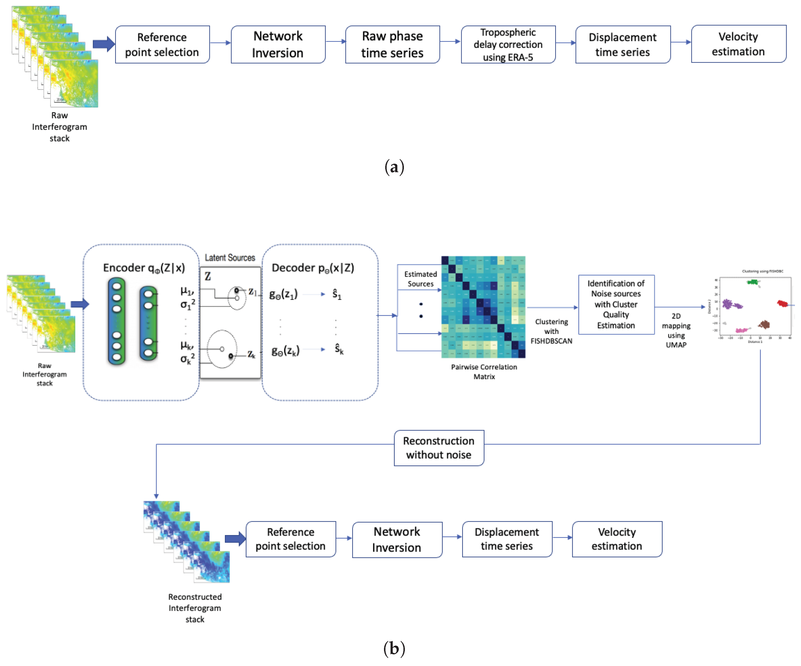
Our method of correction of atmospheric delay from a time series of interferograms follows the following steps as shown in Figure 1. The first step Section 2.1 uses the blind signal separation approach using a variational autoencoder, inspired by the work by [22] to isolate the signals from a time series of interferograms. The second step Section 2.2 utilizes a clustering approach using the FISHDBC algorithm to cluster the recovered sources, and the unclustered elements are classified as noise and the interferograms are reconstructed back with all the recovered sources without the noise elements. The third step Section 2.3 is an integration of this VAE-based noise reduction algorithm in the MintPy pipeline for swift processing of InSAR time series. These three steps are discussed in more details in the following subsections. In this work, as input data, we utilize a time series of interferograms having different values of temporal baseline.

2.1. Variational Autoencoder

Interferograms can be considered as a mixture of signals, and with multiple latent signals combined in unknown quantities in an interferogram, recovering the original signals can be viewed as a problem of blind signal separation [9,10]. This analysis approach [23] reshapes the interferograms such that the spatial dimension is treated as a single dimension and the individual interferograms are concatenated in time.

The variational autoencoder (VAE) [24] (Figure 2) algorithm, adapted from the work by [22], produces an inference of latent source encodings from mixed signal data and independently generates high-dimensional source signals. This unsupervised blind source separation (BSS) problem involves estimating the underlying sources from a mixture of signals, without knowing the true number of sources and without clean target source signals for training the model. According to the idea of blind source separation, this method involves a multi-dimensional vector x made from a sum of M sources s_m plus noise $ϵ$. Given this mixed signal x, the goal is to infer a certain number (K) of estimated sources ŝ_k, where M is less than or equal to K. Since the exact value of M is unknown, it is assumed that the mixture comprises at most K sources. In this completely unsupervised method, strong prior information is required to make assumptions or to model the sources and learn prior source information from the data itself. In this approach, prior information is learned from the training dataset of mixtures, which in this case are the time series of interferograms, through the encoder, which is an inference model, and the decoder, which is a deep generative model. The encoder separates the mixture into latent sources and the decoder independently generates a signal from each latent source. So, to summarize, input to the variational autoencoder (VAE) is a single-channel mixed signal, and the output consists of the individual source signals. The extracted signal sources can be added together to provide an estimate $\hat{\mathrm{x}}$ of the data mixture.

Variational autoencoders (VAEs) are particularly well-suited for unsupervised blind signal separation (BSS) due to their ability to model complex, high-dimensional data through a probabilistic framework [22]. By learning a latent space representation of the data, VAEs can disentangle the underlying sources of a mixed signal. Unlike traditional autoencoders, which only learn deterministic mappings, VAEs model both the latent variables and their distributions, making them robust to uncertainty, noise, and incomplete data. This probabilistic nature allows for VAEs to effectively separate sources even when the mixing process is nonlinear, a common characteristic in real-world signal separation tasks. This notion was also reinforced in a recent paper by [25], where the authors introduce a novel approach to BSS problems in the VAE framework.

In comparison to other models such as independent component analysis (ICA) [9,10] and non-negative matrix factorization (NMF), VAEs offer greater flexibility, as they do not rely on assumptions of linearity or statistical independence. Additionally, VAEs can handle the nonlinear relationships often present in BSS problems [22]. While ICA and NMF excel in specific scenarios, they are limited in their ability to model nonlinear mixtures. VAEs, through their structured latent space and unsupervised learning approach, provide a powerful tool for blind signal separation without the need for labeled data, making them highly effective for complex separation tasks where traditional methods may fall short [25].

2.1.1. Encoder

The latent sources from the encoder are represented as z_k for each estimated source k. Let Z = [z_k]^K_k=1 represent the concatenation of all the latent source variables estimated. Inferring Z from data x provides estimates of latent sources z_k, which are subsequently used to generate source signals ŝ_k in the decoder and thus achieve source separation. Variational inference is used to approximate the posterior distribution over the latent variables given the data [22]. The approximate posterior q_$\varphi$ is defined as

$$q_{\varphi }(Z|x)=N(Z|{\mu }_{\varphi }(x),{\sigma }_{\varphi }^2(x)),$$

(1)

where N represents the Gaussian distribution with mean $\mu$ and variance $\sigma$².

2.1.2. Decoder

The decoder or the generator function gΘ consists of parameters Θ to decode the latent source z_k into its higher-dimensional signal ŝ_k, such that ŝ_k = gΘ(z_k). The estimate of the mixed data is given by the sum of the source signals $\hat{\mathrm{x}}$ = ${\sum }_{k=1}^K$ŝ = ${\sum }_{k=1}^{K}g\theta (zk)$. For reconstruction, instead of using a Gaussian likelihood (l₂ loss), the Laplace likelihood (l₁ loss) is recommended by [26] for precise reconstructions. Isotropic Gaussian priors are defined over each source’s latent variable,

$$p(Z)=\prod _{k=1}^{K}p(z_k)=\prod _{k=1}^{K}N(z_k|0,I),$$

(2)

where p is the likelihood of the Z. This prior assumes that each element is independently varying and helps in separating the variation factors in the data. The variational lower bound was maximized by the equation given in Equation (3) [22], where dataset X = x⁽ⁿ⁾, for n = 1 to N, consists of N i.i.d. samples.

$$L(\theta ,\varphi ;X)=\sum _{n=1}^N{(ln{p}_{\theta }(x^n|Z))}_{q_{\varphi }}-D_{KL}(q(Z|x^{(n)}\left|\right|p(Z))$$

(3)

Equation (3) simplifies into two terms: the first term is the expected log-likelihood that minimizes the reconstruction error, and the second term is the negative Kullback–Leibler divergence (KLD) [27] between two entities, the approximate posterior and the prior that minimizes the difference between the two distributions. In variational autoencoding, it is common to assume a Gaussian approximate posterior as it enables simple Monte Carlo estimation of the expected log-likelihood [22].

2.1.3. Architecture

The encoder and decoder architecture mirrors the structure described in [22]. Both the encoder and decoder consist of five fully connected feed-forward neural network layers. Each linear layer is followed by a ReLU activation function and batch normalization. In the encoder, the hidden units progressively decrease after each layer, transitioning from the high-dimensional, vectorized input to a low-dimensional latent variable. The output of the final layer approximates the posterior mean $\mu$ and log-variance ln${\sigma }^2$ of Z. In contrast, the decoder’s hidden units increase after each layer, starting with the sampled latent source z_k and progressing in reverse order. The last fully connected layer is followed by a sigmoid activation function to output a source signal ŝ_k. Source signals are summed to produce the expected value of the data mixture ${\hat{\mathrm{x}}}_{\mathrm{k}}$.

2.2. Clustering

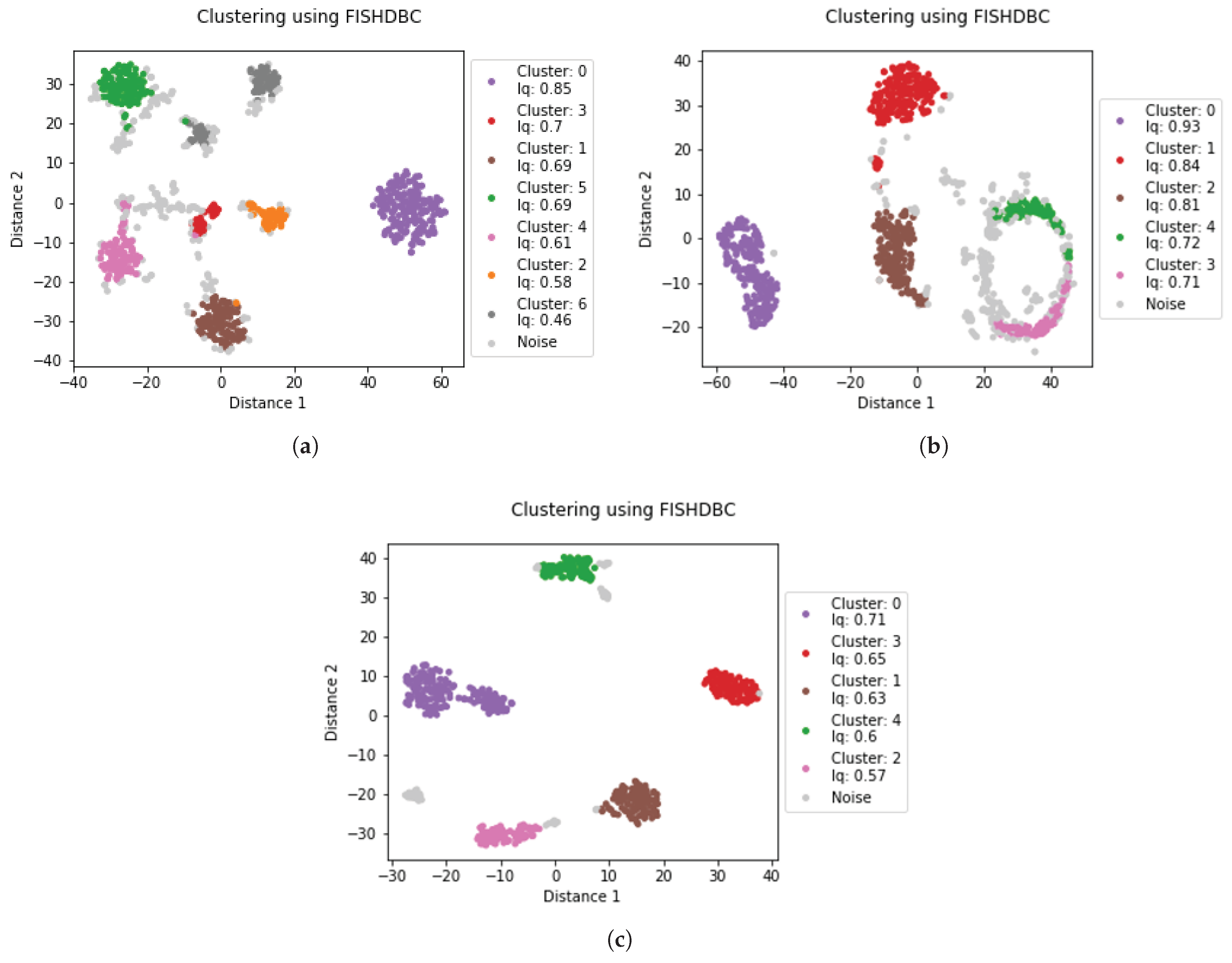
Clustering algorithms can be utilized to identify which estimated source signals ŝ_k are similar and label these as belonging to a cluster, similar to the method implemented in [9]. In case of images, where the samples have equal variables as pixels, clustering a few samples in a very high dimensional space becomes very difficult. As mentioned in [28], in this case, it becomes necessary to use the absolute value of the correlation between source pairs as a similarity measure to get a similarity matrix S. For clustering, the Flexible, Incremental, Scalable, Hierarchical Density-Based Clustering for Arbitrary Data and Distance (FISHDBC) [29] algorithm is used. This is an upgrade of the HDBSCAN algorithm, which was used in the paper by [9], in terms of scalability and because of a regularization effect [29]. Similar to the method mentioned in [9], the FISHDBSC algorithm also gives an estimate of the stability of the clusters in terms of a metric known as the cluster quality index (Iq) and also determines the optimal number of clusters to be formed. The cluster quality index Iq is measured as the difference between the mean of the distances inside the cluster, and the mean distance between items in the cluster and out of the cluster [9], which measures the robustness of each recovered source. The main advantage and primary reason for using this algorithm is that it is able to determine points that do not belong to any cluster and to label these as noise, which are then removed from the data. The cluster points with the lowest Iq are labeled as noise. The interferograms are then reconstructed without the source signals identified in the noise cluster. For 2D representation of the clustering, the Uniform Manifold Approximation and Projection for Dimension Reduction (UMAP) algorithm [30] is used. UMAP is a dimension reduction technique that can be used for visualization similarly to t-SNE [31] used in [9] but also for general nonlinear dimension reduction. This algorithm is used to create the 2-D plot shown in Figure 7, in which the points that represent each recovered source are colored depending on which cluster they are a member of or if they are noise. This plot is useful to qualitatively ascertain the distribution of the noise elements in the data and to highlight that, since these points cannot be identified into a particular cluster group, removal of these points will enhance the importance of the recovered sources and will help in deformation extraction using the reconstructed interferogram time series.

2.3. Integration into MintPy

The Miami INsar Time-series software in PYthon (MintPy) is an open-source package for InSAR time-series analysis. In MintPy version 1.6.2, it is possible to create workflows or pipelines for reading a stack of interferograms (coregistered and unwrapped) and geometry files, like the Digital Elevation Model (DEM), lookup table, and incidence angle, and producing ground surface displacement in the line-of-sight direction using the SBAS method. The workflow modules for MintPy are described in Figure 3. Each module is responsible for a specific task, like reading the unwrapped interferograms, referencing all of them to the same coherent pixel (reference point), calculating the phase closure and estimating the unwrapping errors, inverting the network of interferograms into a time series, calculating the temporal coherence to evaluate the quality of inversion, removing the phase ramps, correcting DEM error, correcting for stratified tropospheric delay (using global atmospheric models), and finally estimating the velocity.

In our approach, we have implemented the VAE-clustering module as an extra pipeline feature, before providing the input for the standard MintPy pipeline. The interferometric stack after correction of noise using the VAE-clustering method is then read by the MintPy module, and successive workflows are performed. For comparison, we utilize two different workflows:

• First, with the original uncorrected interferograms as inputs and keeping the rest of the modules the same and estimating the tropospheric delay using the delay maps acquired from ERA5. In this method, the tropospheric phase delay of the interferograms was estimated by subtracting the ZTD maps from the original phase of the interferograms. This data is downloaded for the corresponding interferogram dates from the CDS website [32,33,34,35]. To account for residual orbital errors, the original interferograms were corrected from a linear trend in range. This is implemented as a module in MintPy before estimating the velocity.
• Second, by reducing the noise of the interferograms using the VAE-clustering method, then providing the corrected interferogram as input to the MintPy module, and finally estimating the velocity. The step for correcting the stratified tropospheric delay using ERA5 was removed in this workflow.

The velocities estimated by these two methods are compared and analyzed. The workflow is described in Figure 3.

3. Data

3.1. Mashhad, Iran

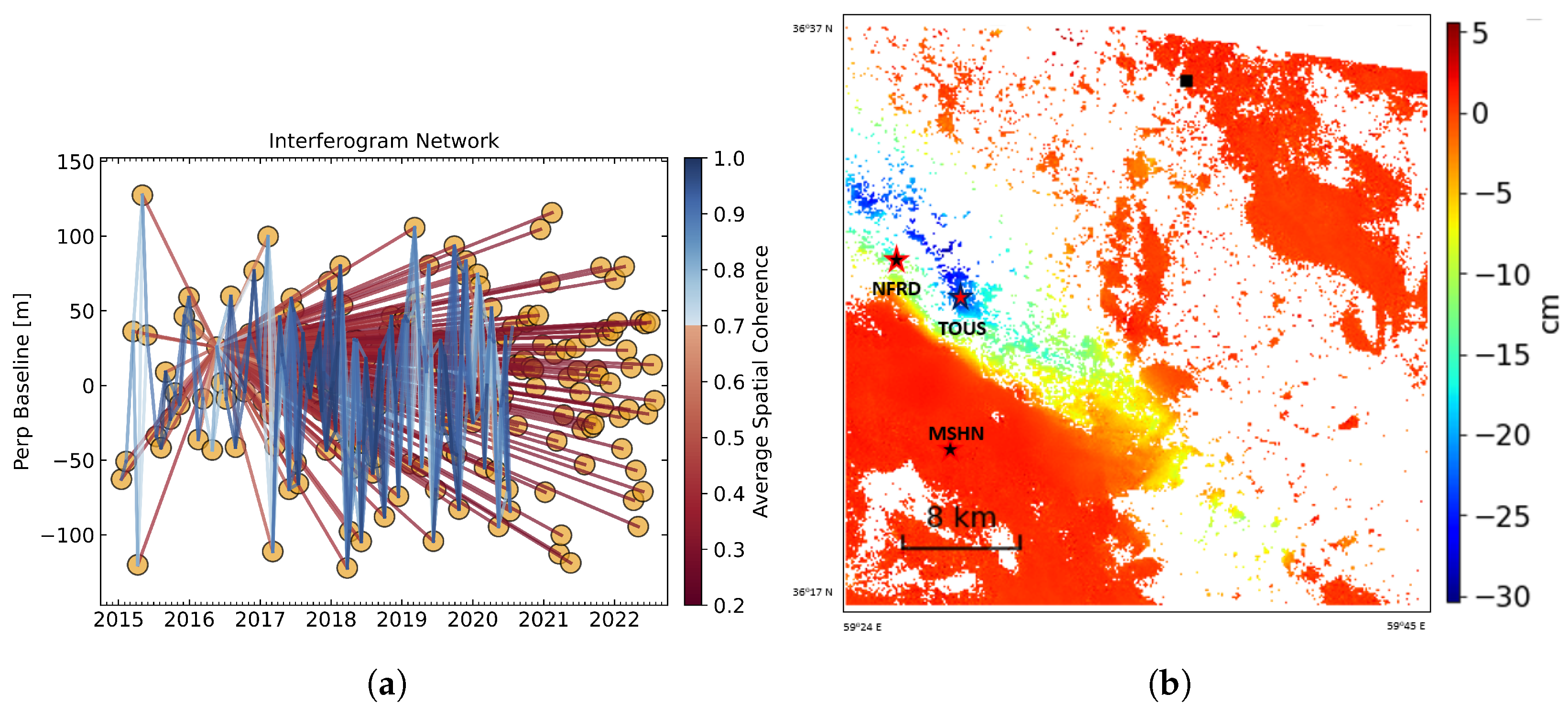
Previous PS-InSAR studies have identified significant subsidence in Mashhad between 2014 and 2017, with two deformation bowls located near GPS stations NFRD and TOUS [36]. Building on this work, we focused on the area surrounding NFRD, as TOUS has been inactive since 2011.

We used Sentinel-1 descending pass data from 2015 to 2021, processed via the ASF HyP3 cloud platform using the Small Baseline Subset Analysis (SBAS) method. This approach enabled rapid, large-scale interferogram generation (≈500 interferograms) without the storage and computational demands of local processing.

GPS displacement measurements from NFRD (same period) were utilized as validation datasets, to be compared with InSAR-derived displacements after atmospheric corrections. The MSHN GPS station, located in an area of negligible deformation [36], was used as the reference site. Using MSHN ensured that displacement estimates at NFRD reflected relative deformation and removed any regional offsets. The details of the SAR acquisition parameters and GPS stations for Mashhad are given in

Table 1. SAR acquisition parameters and GPS stations for Mashhad.

Parameter	Value
Track (Path)	93
Frame	472
Orbit	43,565
Flight Direction	Descending
Time Span	2015–2021
Interferograms	≈500
Reference GPS Station	MSHN
Active GPS Station for Validation	NFRD

.

Figure 4 shows the SBAS network and an example interferogram covering the area of interest.

3.2. Tehran, Iran

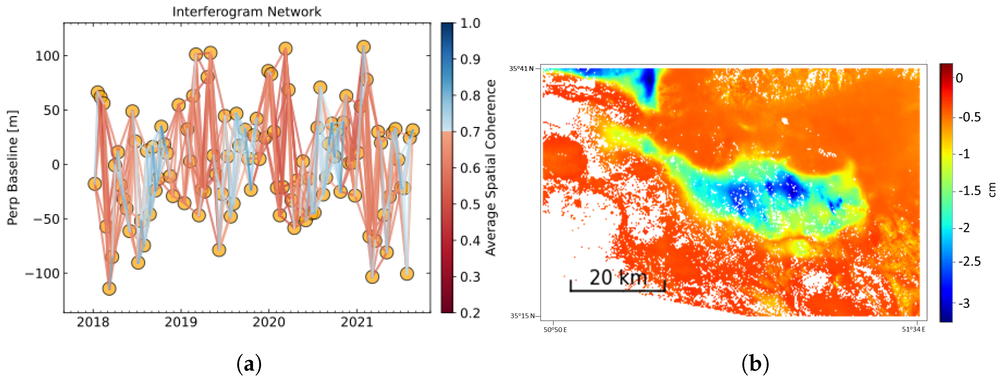
A previous InSAR time-series analysis of Tehran [37] identified three primary subsidence zones: (1) the western Tehran Plain, (2) the vicinity of Tehran International Airport, and (3) the Varamin Plain southeast of the city. For this study, we focused on an area west of Tehran, overlapping with one of the documented subsidence zones to ensure comparability with earlier findings.

We used Sentinel-1 ascending pass data from 2018 to 2021, generating approximately 500 interferograms with varying temporal baselines. Processing was carried out using the SBAS method on the ASF HyP3 cloud platform. This cloud-based approach enabled rapid, consistent, and scalable processing without the need for local computational resources, ensuring methodological uniformity with our Mashhad dataset. The details of the SAR acquisition parameters for Tehran are given in

Table 2. SAR acquisition parameters for Tehran.

Parameter	Value
Track (Path)	78
Frame	52
Orbit	26,179
Flight Direction	Ascending
Time Span	2018–2021
Interferograms	≈500
Processing Method	SBAS via ASF HyP3

.

Figure 5 shows the SBAS network and an example unwrapped interferogram of the area of interest.

3.3. Acapulco, Mexico

On 8 September 2021, a magnitude 7.0 earthquake struck near Acapulco, Guerrero, Mexico [38], producing significant coseismic deformation. To analyze postseismic surface changes, we selected an area of interest encompassing the earthquake epicentral region.

We used Sentinel-1 data spanning January 2021 to April 2022 and constructed approximately 100 interferograms with temporal baselines of 6, 12, 18, and 24 days. Data processing employed the SBAS method via the ASF HyP3 cloud platform, maintaining consistency with our Mashhad and Tehran datasets and enabling efficient handling of large data volumes. The details of the SAR acquisition parameters for Acapulco are given in

Table 3. SAR acquisition parameters for Acapulco.

Parameter	Value
Track (Path)	58
Flight Direction	Ascending
Time Span	January 2021–April 2022
Interferograms	≈100
Temporal Baselines	6, 12, 18, 24 days
Processing Method	SBAS via ASF HyP3

.

Figure 6 shows the SBAS network and an example coseismic interferogram from before and after the earthquake.

4. Training Details

The VAE-clustering algorithm was then applied on all the interferogram stacks from Mashhad, Tehran, and Mexico. The model was trained on an NVIDIA GPU with an Adam optimizer. The batch size was kept at 128 and the learning rate started at 1 $\times {10}^{-4}$ and decayed exponentially by 0.01% per epoch for training the model. As mentioned in [22], we employed a similar technique of multiplying the KLD with a factor $\mathrm{\beta }$ that increased linearly from 0 to 0.5 over the first 100 epochs. This was performed to avoid posterior collapse early in training.

Since the VAE model used was completely unsupervised, no ground truth data was required while training. The total loss function, comprising the reconstruction error and the KLD between the original interferogram and the reconstructed interferogram, from the summation of the estimated sources (Equation (3)), was calculated at each forward pass and the model parameters were updated during the backward pass.

For the cases of Mashhad and Tehran, around 300 interferograms were randomly selected for training the corresponding models. Similarly, for the Acapulco dataset, 70 out of the 100 interferograms were selected as the training set. A total of 50 random interferograms from the Mashhad and Tehran datasets and 10 random interferograms from the Acapulco dataset was selected as the validation set. Training was stopped once the total loss of the validation sets converged, after about 500 epochs, in all cases. Once the corresponding VAE model was trained, the whole interferogram stack, for each dataset, was given as input to the pipeline. During input, each interferogram was flattened into 1-dimensional vectors and the output estimated source signals were also flattened 1-dimension versions. A batch size of 128 interferograms were used while training and the set of interferograms were ordered sequentially by date, during both training and validation.

As shown in Figure 1, the VAE first isolates the different estimated sources from the interferogram stack, then a pairwise correlation matrix is calculated from the recovered source signals, and then the estimated sources are clustered and the noise elements are identified. The noise elements were then removed and the interferogram stack was reconstructed with noise corrected, which was then automatically transferred to the subsequent pipelines in MintPy, for velocity estimation. For comparison with the correction based on ERA5, in a separate MintPy workflow, as depicted in Figure 3, the original interferogram stack was provided as input, the network was inverted, and the ERA5 data was downloaded from the CDS portal. The noise correction using the downloaded ERA5 data was performed, and then, the velocity of displacement was calculated.

5. Results

For all three datasets, the clustering results with the noise labeled are shown in Figure 7. The clusters highlighted by the points in colors other than gray (indicating noise) can represent other source signals, like the deformation source, topographically correlated atmospheric phase screen, or even the east–west phase gradient. The exact identity of these sources can be identified if the magnitude of these individual sources are plotted over time, like in [9] or [10]. In this study, the focus is mainly on removing the noise from the interferograms.

5.1. Results from Mashhad

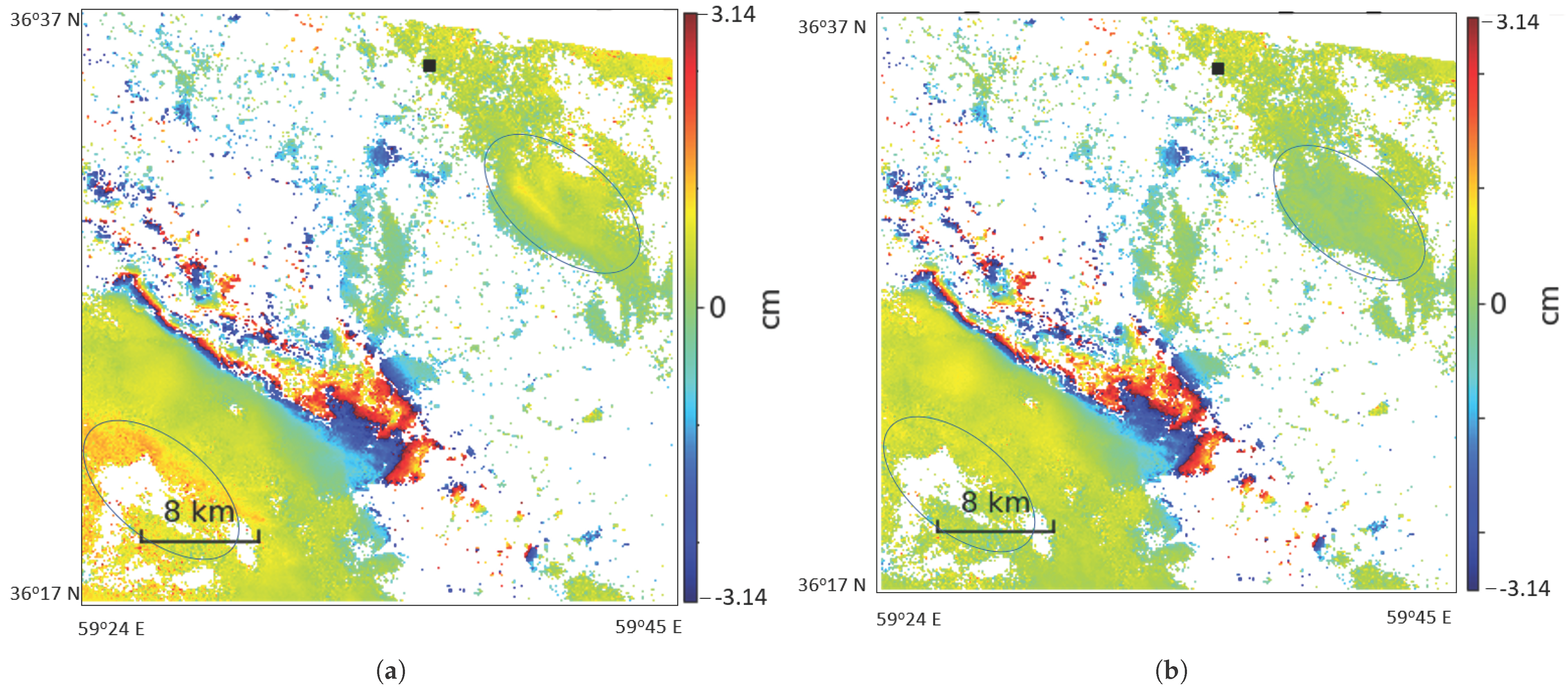
Figure 8 shows an example of a wrapped interferogram in Mashhad between dates 22 May 2016 and 23 July 2016. Figure 8a shows the wrapped interferogram after correction using the ERA5 model while Figure 8b shows the interferogram after correction using the VAE-clustering method. As can be seen from the figure, the VAE-clustering method is able to remove some of the residual noise in Figure 8b, which can still be seen in Figure 8a, after correction using the ERA method.

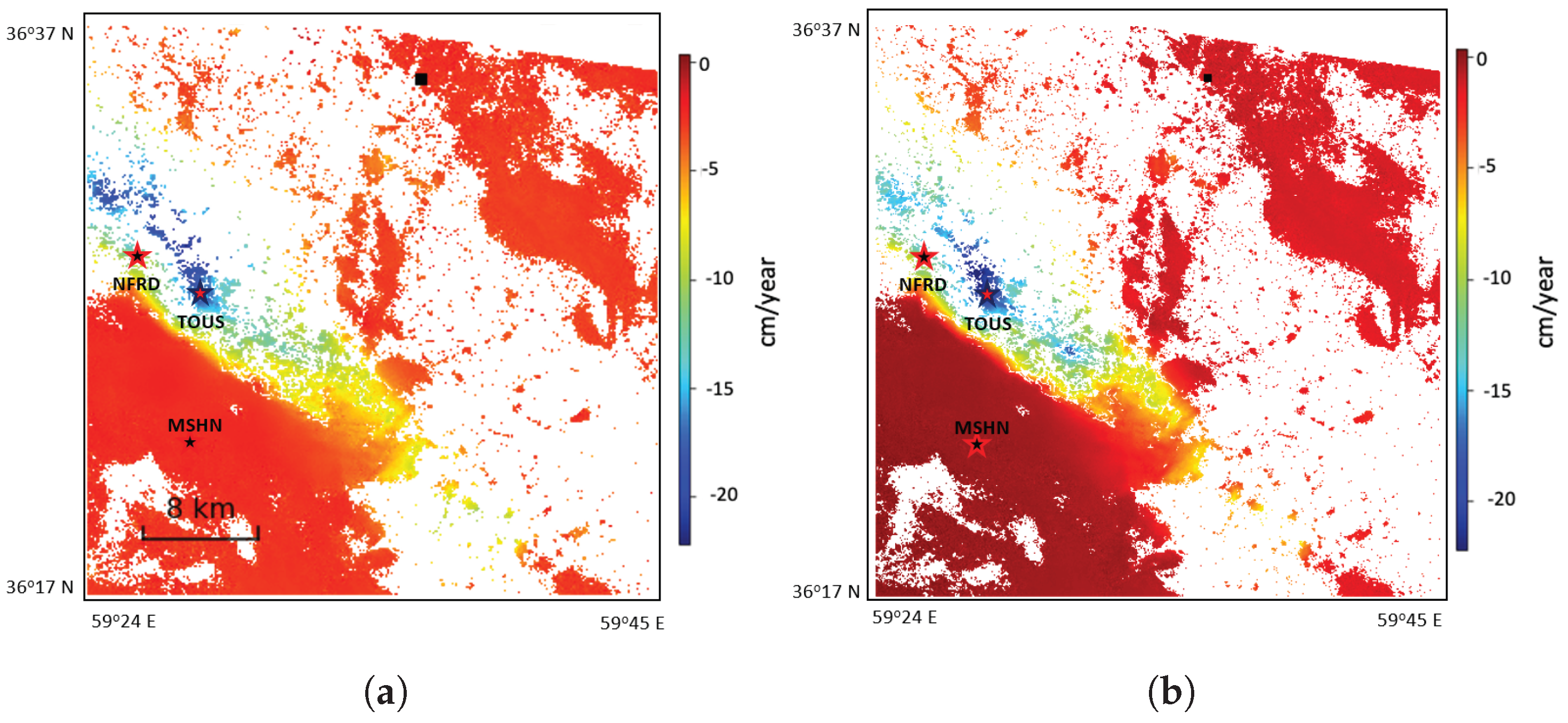
The velocity calculated using the ERA5 correction and the VAE-clustering correction was then compared, as shown in Figure 9. As it can be seen from the two velocity maps, there has been sustained subsidence in the area over the period of seven years.

Taking the area around the NFRD station into consideration, the displacement time series is plotted in Figure 10 for both cases, the ERA5 corrected result and the VAE-clustering corrected result. The vertical GPS displacement measurement, calculated from the NFRD station, relative to the measurement at the MSHN station, is also plotted in Figure 10a,b, from 2015 to 2021, for comparison to the InSAR measurements. There has been a cumulative displacement of around 40cm from 2015 to 2022, according to Figure 10. Similarly, taking the area around the TOUS station into consideration, the displacement time series is plotted in Figure 11 for both cases, the ERA5 corrected result and the VAE-clustering corrected result. As it can be seen, in this area, there has been a cumulative displacement of around 140cm from 2015 to 2022, according to Figure 11.

In the results shown in Figure 9, the velocity after correction using the ERA5 model amounts to 5.58 cm per year, but after correction using the VAE-clustering method the estimated velocity is around 5.07 cm per year. This is also corroborated by the findings of [36]. However, the time series after correction using the ERA5 model in Figure 10a still shows a high standard deviation of 1.58 cm per year, but this is corrected in the time-series result from the VAE-clustering method in Figure 10b, and the standard deviation in this case is also 0.25 cm per year. Thus, in this case, the precision in velocity estimates improved by approximately 84%, in comparison to the ERA5 corrected method. The GPS measurement also shows more agreement with the InSAR time series after correction using the VAE-clustering method in Figure 10a than in Figure 10b. Thus, here the GPS in situ measurement helps in validating the performance of the model for this particular case study.

Similarly, in the results shown in Figure 11, the velocity after correction using the ERA5 model amounts to 20.28 cm per year, but after correction using the VAE-clustering method the estimated velocity is around 19.87 cm per year. This is also corroborated by the findings of [36], which serves as an in situ validation for the model performance. However, the time series after correction using the ERA5 model in Figure 11a still shows a high standard deviation of 1.37 cm per year, but this is corrected in the time-series result from the VAE-clustering method in Figure 11b and the standard deviation in this case is also 0.15 cm per year; this is an improvement of 89% per year in terms of the standard deviation, in comparison to the ERA5 corrected method.

5.2. Results from Tehran

Figure 12 shows an example of the wrapped interferogram between dates 10 January 2020 and 10 March 2020 in Tehran. Figure 12a shows the wrapped interferograms after correction using the ERA5 model, while Figure 12b shows the interferogram after correction using the VAE-clustering method. As can be seen from the figure, the VAE-clustering method is able to remove some of the residual noise in Figure 12b, which can still be seen in Figure 12a, after correction using the ERA method.

The velocity calculated using the ERA5 correction and the VAE-clustering correction was then compared, as shown in Figure 13. As it can be seen from the two velocity maps, there has been sustained subsidence in the area over the period of three years.

Taking this area into consideration, the displacement time series is plotted in Figure 14 for both cases, the ERA5 corrected result and the VAE-clustering corrected result. As it can be seen, in this area, there has been a cumulative displacement of around 100 cm in three years from 2018 to 2021, according to Figure 14b, which is the resultant time series after correction using the VAE-clustering method. The time series after correction using the ERA5 model shows that the total cumulative displacement is around 105cm, but this may be an overestimation due to the residual noise still present as shown in Figure 14a.

In the results shown in Figure 14, the velocity after correction using the ERA5 model amounts to 27.29 cm per year, but after correction using the VAE-clustering method the estimated velocity is around 25.32 cm per year. This is also corroborated by the findings of [37], where the authors estimated that there was subsidence of around 25 cm per year from 2015 to 2017. In Figure 14a, the time series after correction using the ERA5 model still shows a seasonal trend with a standard deviation of 1.24 cm per year, but this seasonal trend is corrected in the time-series result from the VAE-clustering method in Figure 14b and the standard deviation in this case is also 0.31 cm per year. Thus, in this case, we observe an improvement of 75% in terms of the standard deviation, in comparison to the ERA5 corrected method.

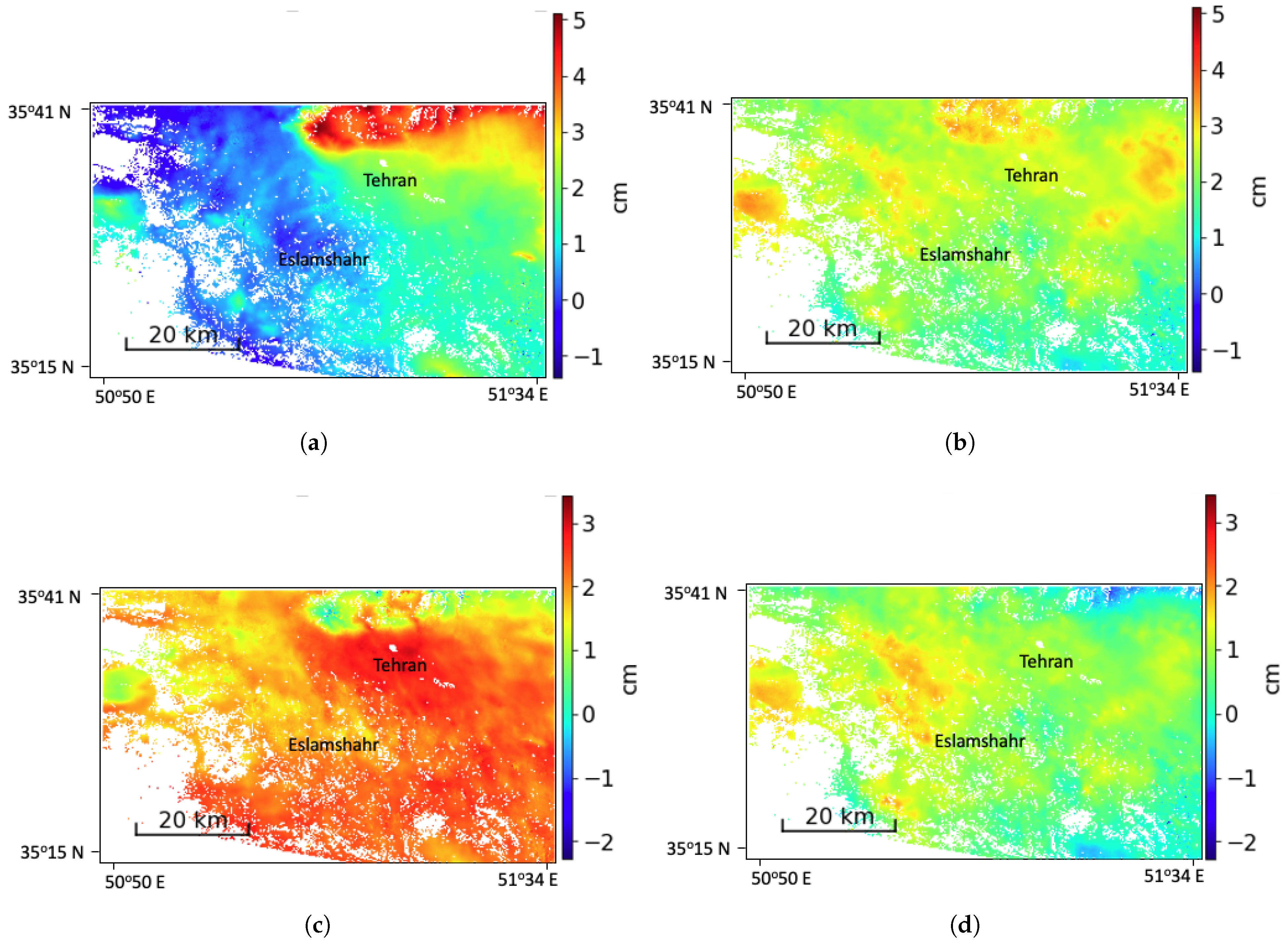
For a demonstration of atmospheric error correction, interferograms of short temporal baselines like a 12-day interval are selected. In Figure 15a–d, 12-day interferograms of dates 16 November 2018–28 November 2018, and 17 March 2021–29 March 2021 are shown, with both before corrected as well as after VAE-clustering-based corrected versions. As can be seen from the figures, the VAE-clustering-based method improves on the corrections by reducing the residual noise. Due to the high rate of deformation in this area, even in 12-day short-term interferograms, some deformation is still visible, like in Figure 15d.

5.3. Results from Acapulco, Mexico

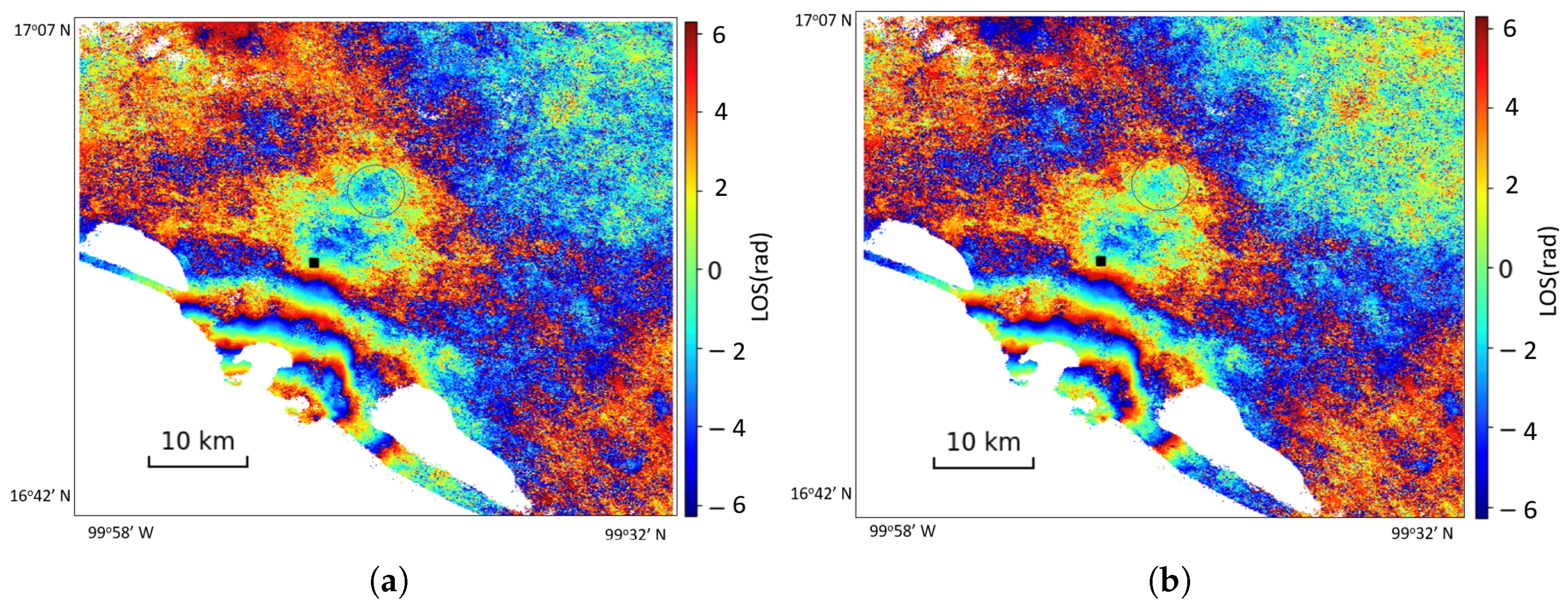
Figure 16 shows the rewrapped interferogram between dates 4 September 2021 and 16 September 2021. The interferogram was rewrapped to the range −2 pi to 2 pi, for better visualization of the fringes, denoting 20 cm of displacement for better visualization. (a) shows the wrapped interferogram after correction using the ERA5 model while (b) shows the interferogram after correction using the VAE-clustering method. The interferograms have been rewrapped after correction. As it can be seen from the two figures, in both cases, the major deformation was near Acapulco, where the earthquake occurred, and especially in the area south of Acapulco. As can be seen from the figure, the VAE-clustering method is able to remove some of the residual noise in (b), which can still be seen in (a), after correction using the ERA5 method.

The cumulative unwrapped displacement time series after correction using the VAE-clustering method is shown in Figure 17. There is no significant difference between the interferograms from 7 January 2021 to 14 September 2021. However, starting from 16 September 2021 onwards, we observe an uplift of nearly 20 cm related to the earthquake, which remains as a dominant signal in the postseismic period.

Taking the area south of Acapulco into consideration, the displacement time series is plotted in Figure 18 for both cases, the ERA5 corrected result and the VAE-clustering corrected result, for both pre- and post-earthquake time periods. As it can be seen, in this area, there has been a cumulative uplift of around 20 cm, based on the offset in the displacement right after the earthquake, in September 2021, according to Figure 18b, which is the resultant time series after correction using the VAE-clustering method. In Figure 18a, the time series after correction using the ERA5 model shows a standard deviation of 0.24 cm per year before the earthquake and 1.81 cm per year after the earthquake. But in the time-series result from the VAE-clustering method in Figure 18b, the standard deviation is 0.05 cm per year before the earthquake and 0.85 cm per year after the earthquake. Thus, in this case, we observe an improvement of 53% in terms of the standard deviation for estimating the postseismic velocity, in comparison to the ERA5 corrected method. These results are also corroborated in the paper by [39], which serves as an in situ validation for our model with respect to this case study.

6. Discussion

Our study with Sentinel-1 data showed that ERA5 is not able to reduce the tropospheric phase delay completely in the interferometric measurement. Our proposed method based on variational autoencoders improves the corrections of the tropospheric phase delay in the interferometric measurement, compared to the ERA5 model. This method can be also trained on new data on the fly and thus capture any changes in the dataset and this will be reflected in the model as well. Also, since this technique is completely unsupervised, it does not require any prior ground truth or training data to train the model.

Also, the ASF cloud processing platform offers a streamlined and scalable environment for SAR data handling. This cloud-based framework enables direct formation of unwrapped interferograms without the need for local computational infrastructure, eliminating the traditionally high storage, processing time, and hardware requirements associated with InSAR workflows. By leveraging HyP3, large volumes of Sentinel-1 data can be accessed, processed, and quality-checked entirely online, facilitating near-real-time interferogram generation and enabling rapid iteration of analysis workflows. This approach not only accelerates the overall processing pipeline but also lowers the entry barrier for large-scale InSAR analysis, making advanced interferometric processing more accessible to the scientific and operational monitoring community. Any new data can be processed in the ASF cloud processing platform to construct the interferograms. Subsequently, this interferogram stack can be provided as input to the MintPy pipeline as described in Figure 3 for estimation of velocity and deformation on the fly.

Also, our variational autoencoding-based approach offers a solution for unsupervised blind source separation from interferograms. In this approach, using an encoder and decoder for disentangling sources in a low-dimensional probabilistic latent space and generating the estimated sources independently using the same deep neural network ensures that the size and the memory consumption of the network remains consistent regardless of the number of model sources, which is an advantage over existing methods that use different networks for each source. It may be that a simplified version of the model with a few hidden layers and Gaussian assumptions may have been sufficient for separation of sources from simpler mixed signals, but this more precise model is necessary for signal separation from complex mixed signals, like interferograms.

When using VAEs to isolate the estimated signals, the use of the clustering algorithm, the automatic identification of the noise signals by the FISHDBC algorithm, and subsequent 2D visualization using UMAP representation requires minimal intervention from a human user and thus helps in the recovering the original interferogram time series without the noise elements. The utilization of the MintPy platform to seamlessly integrate this model as a pipeline module also benefits from automatization of the whole process from interferogram formation to velocity estimation. In this case also, the fact that the MintPy software is entirely based on Python is deemed of great advantage as any machine learning or deep learning model can be integrated into the workflow, thus providing for further future development and innovations in this topic automatic correction and velocity estimation from interferometric time series.

6.1. Comparison of Performance of VAE-Clustering Method with Adaptive Localized Phase Topography Correction Method

In the publication [40], the author introduced an approach for mitigating tropospheric delays by applying localized phase-topography corrections to interferograms. This method estimates linear coefficients within smaller spatial windows and uses bicubic interpolation to generate a smoothly varying correction surface. An iterative masking approach is applied to exclude significant deformation areas during coefficient estimation, thereby improving accuracy. The process is repeated until the broad-scale and stratified tropospheric effects are reliably corrected. Residual high-frequency tropospheric noise, assumed to be temporally uncorrelated, is reduced by averaging multiple interferograms, enhancing the overall signal-to-noise ratio of the displacement time series.

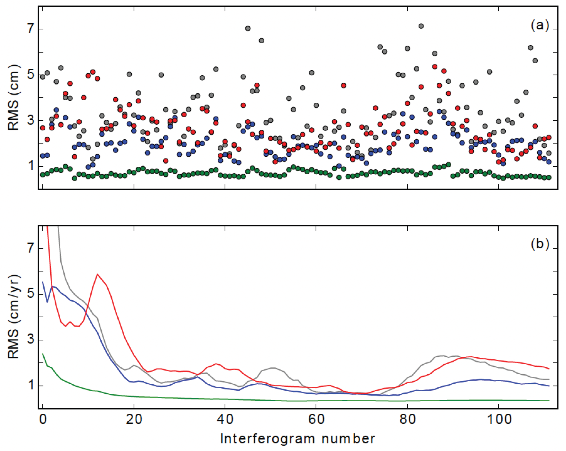
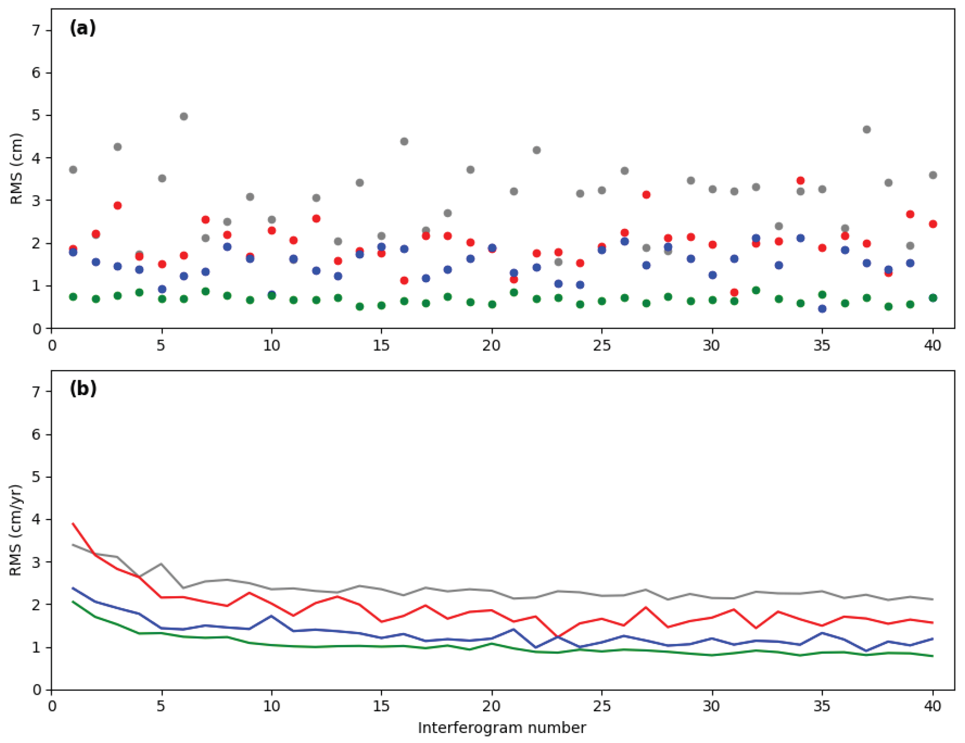
This adaptive algorithm was separately applied to more than 100 random interferograms from the Tehran dataset, around 250 interferograms from the Mashhad dataset, and 40 interferograms from the Acapulco, Mexico, dataset for removing the tropospheric noise. Three versions of the corresponding interferograms were also selected: the interferogram without any applied corrections, the interferograms after correction using the ERA5 model, and the interferograms after correction using the VAE-clustering method. The standard deviation and the RMS of the average velocities of the individual interferograms corrected using the different approaches were calculated for both datasets. The results have been plotted in Figure 19, Figure 20 and Figure 21. For all cases, the RMS of the individual interferograms are improved continuously from the uncorrected, to the ERA5 corrected, to the adaptive method corrected, and finally the VAE-clustering corrected versions. The RMS of the average velocities also follow a similar pattern.

The VAE-clustering-based correction significantly improved the results by separating the localized displacements from the background errors. It removed most parts of the tropospheric errors from the individual interferograms and reduced the RMS of them to lower than 1 cm. Also to note, the RMS of the average velocity using VAE-clustering correction converges, while in the other three approaches, although the RMS generally decreases, it does not converge. This shows that the tropospheric artifacts are being reduced in the case of the correction by the VAE-clustering method, while for the adaptive methods, although broad-scale and topography-correlated errors from the individual interferograms are diminished, the tropospheric artifacts still remain.

To evaluate the dependency of the remaining errors to the relative distance, at every 10 km interval between 0 and 300 km, 1000 pairs of pixels are randomly sampled. The results for Tehran, Mashhad, and Acapulco, Mexico, shown in Figure 22, Figure 23 and Figure 24 indicate that, for all datasets, when using the original interferograms, the average and standard deviation of the velocity difference increase with distance. Although it flattens from a distance of approximately 100 km, it increases again after a distance of 250 km. The ERA5 correction and adaptive correction decrease the dependency to the relative distance. The VAE-clustering-based correction significantly improves the results and completely removes the dependency to distance.

6.2. Some Cases of Exceptions for the VAE-Clustering Approach

In some cases, e.g., Figure 25, when the displacement signal is not strong, the VAE correction may not perform better than the ERA5 model. In such cases both the ERA5 as well as the VAE-clustering correction method may not be able to completely remove the residual turbulence effect. This can be attributed to the fact that the VAE-clustering method, while clustering the noise sources recovered using the VAE from the interferograms, may not be able to identify all the noise sources and some of these noise elements can be mistaken for deformation sources or other sources of interest and thus not removed while reconstructing the interferograms. One way of mitigating this effect is to increase the number of interferograms when processing and consider interferograms of both short as well as long temporal baselines, as more interferograms of both short as well as long temporal baselines covering the same time period can result in more robust recovery of latent sources as well as more efficient clustering of these sources for better identification of noise elements.

6.3. Analysis and Comparison of Application of Algorithms like ICA, NMF, or PCA to the VAE-Clustering Approach

As discussed in Section 1, algorithms like independent component analysis (ICA), principal component analysis (PCA), and non-negative matrix factorization (NMF) have been utilized till now for unsupervised blind source separation and retrieval of independent source signals. Given this fact, it was quite pertinent to assess the performance of the variational autoencoder on blind signal separation tasks from SAR interferograms compared to these algorithms. As NMF cannot be used on data that contains negative values, this algorithm is not taken into consideration as practical cases of interferograms with non-negative values are quite limited. For an accurate comparison among the different algorithms, only sequential interferograms in the form of a daisy chain are considered for this case. As a result, around 100 interferograms having sequential master and slave dates, thus forming a daisy chain, are samples from the Tehran dataset.

To quantitatively compare different blind signal separation methods (e.g., PCA, ICA, and VAE) applied to SAR interferograms, we use the cumulative root-mean-square (RMS) residual as a standard evaluation metric.

Let ${\varphi }_i^{\mathrm{true}}(x,y)$ denote the original interferometric phase at pixel location $(x,y)$ in the ith interferogram and ${\varphi }_i^{\mathrm{recon}}(x,y)$ the reconstructed phase obtained from the separation method. The point-wise residual is defined as

$$r_i(x,y)={\varphi }_i^{\mathrm{recon}}(x,y)-{\varphi }_i^{\mathrm{true}}(x,y).$$

(4)

To assess overall performance across all interferograms and spatial pixels, we compute the cumulative RMS residual:

$${\mathrm{RMS}}_{\mathrm{cumul}}=\sqrt{{\displaystyle \frac{1}{N_{\mathrm{pix}}·N_i}}\sum _{i=1}^{N_i}\sum _{x,y}{\left[r_i(x,y)\right]}^2},$$

(5)

where

• $N_i$ is the number of interferograms in the dataset;
• $N_{\mathrm{pix}}$ is the total number of pixels per interferogram (e.g., spatial resolution × image size).

This cumulative formulation ensures each interferogram and pixel contributes equally to the final residual measure.

In Figure 26, the cumulative root-mean-square (RMS) residual values are plotted for around 100 sampled interferograms from Tehran, using three methods: spatial ICA, PCA, and VAE in Figure 26a, and the distribution of the RMS residual values for the three methods are shown in Figure 26b. As can be seen from the figure, the VAE performs best among the three methods in terms of signal decomposition and reconstruction.

The reasons behind this result could be that PCA captures variance but may conflate deformation with residual noise and ICA can reduce the RMS residual more effectively when deformation sources are statistically independent, but its success depends on data volume and noise structure. The VAE, on the other hand, when well-trained on representative data, is capable of producing a lower cumulative RMS via nonlinear modeling of deformation signals, especially when evaluated across multiple interferograms and pixels. This cumulative RMS metric thus serves as a rigorous quantitative basis for comparing method fidelity in reconstructing geophysical deformation from SAR interferograms.

6.4. Comparison of Using FISHDBC Clustering Against Clustering Using HDBSCAN

As discussed in Section 1, a choice was made to use FISHDBC for clustering, instead of other prevalent clustering strategies like HDBSCAN. This conclusion stems from the fact that the superiority of FISHDBC is primarily twofold. First, its approximation of HDBSCAN* inherently applies a regularization-like effect, which enhances clustering quality metrics such as AMI and ARI, especially in high-dimensional spaces, by preventing over-fragmentation and promoting coherent clusters [29]. Second, FISHDBC supports arbitrary (potentially non-metric) distance functions and provides scalable, incremental clustering. It eschews the $O(n^2)$ complexity of traditional density-based methods in non-metric spaces and allows for efficient updates as new data arrives [29]. These characteristics make FISHDBC especially effective in scenarios involving high-dimensional, streaming, or domain-specific similarity functions, justifying its superiority over the standard HDBSCAN in terms of the $I_q$-based evaluation.

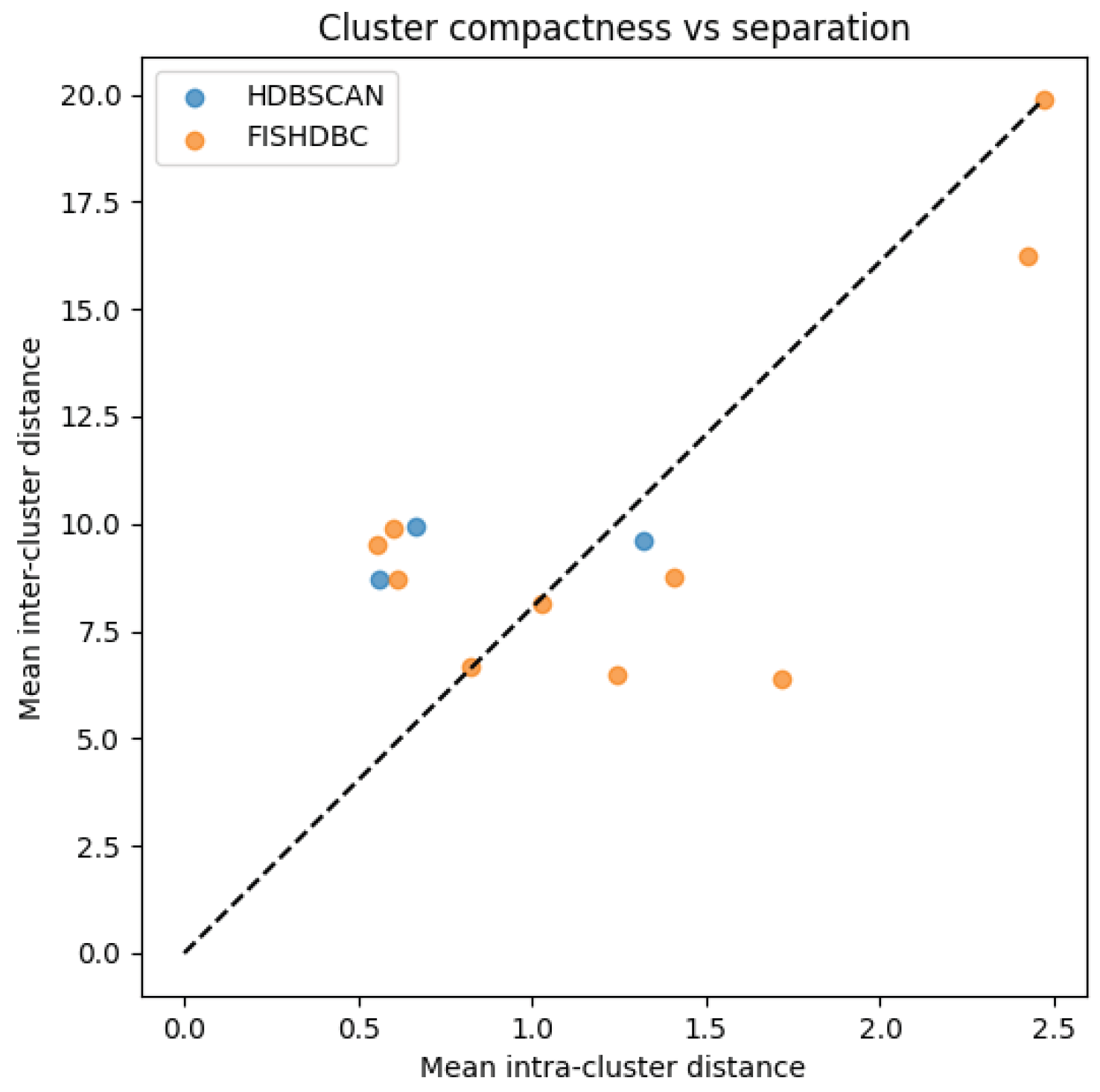
In our evaluation, we analyze clustering efficacy using the cluster quality index $Iq$, defined as

$$Iq={\overline{d}}_{\mathrm{intra}}-{\overline{d}}_{\mathrm{inter}},$$

where a more negative $Iq$ indicates tighter, better-separated clusters. For experimentation, we used the interferograms from the Mexico dataset and executed the MintPy pipeline with both the FISHDBC and HDBSCAN clustering algorithms. Empirically, FISHDBC consistently yielded significantly more negative average $Iq$ values compared to HDBSCAN across various datasets. This performance stems from FISHDBC’s conservative approach to cluster formation—focusing on core cohesion and labeling ambiguous points as noise and thus reducing intra-cluster variance and enhancing inter-cluster separation.

In Figure 27, the cluster compactness versus separation for the HDBSCAN and FISHDBC variants have been plotted. Each point represents a cluster, plotted by its average intra-cluster distance (x-axis) against its average inter-cluster distance (y-axis). Ideal clusters are located toward the lower-right, indicating tight cohesion (low intra) and clear separation (high inter). In our experiments, FISHDBC cluster points are noticeably farther to the lower-right than those from HDBSCAN—demonstrating superior cluster quality (i.e., more negative cluster quality index Iq) due to FISHDBC’s emphasis on core cohesion and effective noise exclusion.

7. Conclusions

In this paper, we presented an unsupervised approach for the problem of tropospheric noise removal in interferograms based on variational autoencoder-based clustering. We built an architecture for automatic detection and removal of noise signals from the interferograms and subsequent integration into a MintPy pipeline for rapid retrieval of velocity and displacement using the SBAS technique. Through the experiments, we showed how our model outperforms the tropospheric noise correction method by the ERA5 model for three case studies: the subsidence in Mashhad, Iran; the subsidence in Tehran, Iran; and the post-earthquake uplift in Acapulco in Mexico. This is testified by the different methods, like comparison of displacement time series and RMSE of the interferograms. This method can be updated dynamically as new data arrives, allowing the model to adapt to evolving patterns in the dataset. Furthermore, because the technique is entirely unsupervised, it does not depend on any labeled ground truth or preexisting training data.

8. Future Work

The blind signal separation method implemented in our approach can also be extended to be applied in source signal separation from SAR interferograms, especially for extraction of deformation signals in InSAR. As a future work, it may be interesting to see how this method performs with regards to deformation signal extraction for detection of volcanic activities, in comparison to statistical methods like ICA which have already been implemented for this purpose as mentioned in the papers ([9,10]). Also, based on the recent work by [25], it will also be worth the effort to implement the parameter-adaptive VAE (PAVAE) and the two variations, homoscedastic PAVAE (Ho-PAVAE) and heteroscedastic PAVAE (He-PAVAE), into the VAE-clustering method and compare their performance with regards to atmospheric noise correction from SAR interferograms.

References

1. Massonnet, D.; Feigl, K. Radar interferometry and its application to changes in the Earth’s surface. Rev. Geophys. 1998, 36, 441–500. [Google Scholar] [CrossRef]
2. Bürgmann, R.; Rosen, P.; Fieldling, E. Synthetic Aperture Radar Interferometry to Measure Earth’s Surface Topography and Its Deformation. Annu. Rev. Earth Planet. Sci. 2008, 28, 169–209. [Google Scholar] [CrossRef]
3. Haghshenas Haghighi, M.; Motagh, M. Sentinel-1 InSAR over Germany: Large-scale interferometry, atmospheric effects, and ground deformation mapping. ZFV—Z. Geodasie Geoinf. Landmanag. 2017, 142, 245–246. [Google Scholar] [CrossRef]
4. Bekaert, D.P.S.; Walters, R.J.; Wright, T.J.; Hooper, A.J.; Parker, D.J. Statistical comparison of InSAR tropospheric correction techniques. Remote Sens. Environ. 2015, 170, 40–47. [Google Scholar] [CrossRef]
5. Li, Z. Interferometric synthetic aperture radar (INSAR) atmospheric correction: GPS, moderate resolution imaging Spectroradiometer (MODIS), and insar integration. J. Geophys. Res. 2005, 110, B03410. [Google Scholar] [CrossRef]
6. Ghosh, B.; Haghshenas Haghighi, M.; Motagh, M.; Maghsudi, S. Using Generative Adversarial Networks for Extraction of Insar Signals from Large-Scale Sentinel-1 Interferograms by Improving Tropospheric Noise Correction. ISPRS Ann. Photogramm. Remote Sens. Spat. Inf. Sci. 2021, V-3-2021, 57–64. [Google Scholar] [CrossRef]
7. Jolivet, R.; Grandin, R.; Lasserre, C.; Doin, M.P.; Peltzer, G. Systematic insar tropospheric phase delay corrections from global meteorological reanalysis data. Geophys. Res. Lett. 2011, 38, L17311. [Google Scholar] [CrossRef]
8. Rouet-Leduc, B.; Jolivet, R.; Dalaison, M.; Johnson, P.A.; Hulbert, C. Autonomous extraction of millimeter-scale deformation in InSAR time series using deep learning. Nat. Commun. 2021, 12, 6480. [Google Scholar] [CrossRef]
9. Gaddes, M.E.; Hooper, A.; Bagnardi, M. Using Machine Learning to Automatically Detect Volcanic Unrest in a Time Series of Interferograms. J. Geophys. Res. Solid Earth 2019, 124, 12304–12322. [Google Scholar] [CrossRef]
10. Ghosh, B.; Motagh, M.; Haghighi, M.H.; Vassileva, M.S.; Walter, T.R.; Maghsudi, S. Automatic Detection of Volcanic Unrest Using Blind Source Separation With a Minimum Spanning Tree Based Stability Analysis. IEEE J. Sel. Top. Appl. Earth Obs. Remote Sens. 2021, 14, 7771–7787. [Google Scholar] [CrossRef]
11. Chen, C.; Dai, K.; Tang, X.; Cheng, J.; Pirasteh, S.; Wu, M.; Shi, X.; Zhou, H.; Li, Z. Removing insar topography-dependent atmospheric effect based on Deep Learning. Remote Sens. 2022, 14, 4171. [Google Scholar] [CrossRef]
12. Anantrasirichai, N.; Biggs, J.; Albino, F.; Bull, D. The Application of Convolutional Neural Networks to Detect Slow, Sustained Deformation in InSAR Time Series. Geophys. Res. Lett. 2019, 46, 11850–11858. [Google Scholar] [CrossRef]
13. Zhou, H.; Dai, K.; Tang, X.; Xiang, J.; Li, R.; Wu, M.; Peng, Y.; Li, Z. Time-series insar with deep-learning-based topography-dependent atmospheric delay correction for potential landslide detection. Remote Sens. 2023, 15, 5287. [Google Scholar] [CrossRef]
14. Zhou, H.; Dai, K.; Pirasteh, S.; Li, R.; Xiang, J.; Li, Z. InSAR Spatial-Heterogeneity Tropospheric Delay Correction in Steep Mountainous Areas Based on Deep Learning for Landslides Monitoring. IEEE Trans. Geosci. Remote Sens. 2023, 61, 5215014. [Google Scholar] [CrossRef]
15. Ma, P.; Yu, C.; Jiao, Z.; Zheng, Y.; Wu, Z.; Mao, W.; Lin, H. Improving time-series InSAR deformation estimation for city clusters by deep learning-based atmospheric delay correction. Remote Sens. Environ. 2024, 304, 114004. [Google Scholar] [CrossRef]
16. Cardoso, J.F. Blind signal separation: Statistical principles. Proc. IEEE 1998, 86, 2009–2025. [Google Scholar] [CrossRef]
17. Huang, P.S.; Chen, S.D.; Smaragdis, P.; Hasegawa-Johnson, M. Singing-voice separation from monaural recordings using robust principal component analysis. In Proceedings of the 2012 IEEE International Conference on Acoustics, Speech and Signal Processing (ICASSP), Kyoto, Japan, 25–30 March 2012. [Google Scholar] [CrossRef]
18. Févotte, C.; Bertin, N.; Durrieu, J.L. Nonnegative matrix factorization with the Itakura-Saito Divergence: With Application to music analysis. Neural Comput. 2009, 21, 793–830. [Google Scholar] [CrossRef] [PubMed]
19. Badeau, R.; Dremeau, A. Variational Bayesian EM algorithm for modeling mixtures of non-stationary signals in the time-frequency domain (HR-NMF). In Proceedings of the 2013 IEEE International Conference on Acoustics, Speech and Signal Processing, Vancouver, BC, Canada, 26–31 May 2013. [Google Scholar] [CrossRef]
20. Hoshen, Y. Towards Unsupervised Single-channel Blind Source Separation Using Adversarial Pair Unmix-and-remix. In Proceedings of the ICASSP 2019—2019 IEEE International Conference on Acoustics, Speech and Signal Processing (ICASSP), Brighton, UK, 12–17 May 2019. [Google Scholar] [CrossRef]
21. Yunjun, Z.; Fattahi, H.; Amelung, F. Small baseline InSAR time series analysis: Unwrapping error correction and noise reduction. Comput. Geosci. 2019, 133, 104331. [Google Scholar] [CrossRef]
22. Neri, J.; Badeau, R.; Depalle, P. Unsupervised Blind Source Separation with Variational Auto-Encoders. In Proceedings of the 2021 29th European Signal Processing Conference (EUSIPCO), Dublin, Ireland, 23–27 August 2021. [Google Scholar] [CrossRef]
23. Calhoun, V.; Adali, T.; Pearlson, G.; Pekar, J. A method for making group inferences from functional MRI data using independent component analysis. Hum. Brain Mapp. 2001, 14, 140–151. [Google Scholar] [CrossRef]
24. Kingma, D.; Welling, M. Auto-Encoding Variational Bayes. arXiv 2014, arXiv:1312.6114. [Google Scholar]
25. Wei, Y.H.; Ni, Y.Q. Parameter-adaptive variational autoencoder for linear/nonlinear blind source separation. J. Civ. Struct. Health Monit. 2024, 15, 1161–1184. [Google Scholar] [CrossRef]
26. Neri, J.; Depalle, P.; Badeau, R. Approximate inference and learning of state space models with Laplace Noise. IEEE Trans. Signal Process. 2021, 69, 3176–3189. [Google Scholar] [CrossRef]
27. Kullback, S.; Leibler, R.A. On Information and Sufficiency. Ann. Math. Stat. 1951, 22, 79–86. [Google Scholar] [CrossRef]
28. Gaddes, M.E. Automatic Detection of Volcanic Unrest Using Interferometric Synthetic Aperture Radar. Ph.D. Thesis, University of Leeds, Leeds, UK, 2019. [Google Scholar]
29. Dell’Amico, M. FISHDBC: Flexible, Incremental, Scalable, Hierarchical Density-Based Clustering for Arbitrary Data and Distance. arXiv 2019, arXiv:1910.07283. [Google Scholar] [CrossRef]
30. Sainburg, T.; McInnes, L.; Gentner, T.Q. Parametric UMAP Embeddings for Representation and Semisupervised Learning. Neural Comput. 2021, 33, 2881–2907. [Google Scholar] [CrossRef] [PubMed]
31. van der Maaten, L.; Hinton, G. Viualizing data using t-SNE. J. Mach. Learn. Res. 2008, 9, 2579–2605. [Google Scholar]
32. Yu, C.; Li, Z.; Penna, N.T.; Crippa, P. Generic Atmospheric Correction Model for Interferometric Synthetic Aperture Radar Observations. J. Geophys. Res. Solid Earth 2018, 123, 9202–9222. [Google Scholar] [CrossRef]
33. Yu, C.; Li, Z.; Penna, N.T. Interferometric synthetic aperture radar atmospheric correction using a GPS-based iterative tropospheric decomposition model. Remote Sens. Environ. 2018, 204, 109–121. [Google Scholar] [CrossRef]
34. Yu, C.; Penna, N.T.; Li, Z. Generation of real-time mode high-resolution water vapor fields from GPS observations. J. Geophys. Res. Atmos. 2017, 122, 2008–2025. [Google Scholar] [CrossRef]
35. Copernicus Climate Data Store, 2022. ERA5: Fifth Generation of ECMWF Atmospheric Reanalyses of the Global Climate. Available online: https://cds.climate.copernicus.eu/ (accessed on 9 September 2025).
36. Khorrami, M.; Abrishami, S.; Maghsoudi, Y.; Alizadeh, B.; Perissin, D. Extreme subsidence in a populated city (Mashhad) detected by PSInSAR considering groundwater withdrawal and geotechnical properties. Sci. Rep. 2020, 10, 11357. [Google Scholar] [CrossRef]
37. Haghshenas Haghighi, M.; Motagh, M. Ground surface response to continuous compaction of aquifer system in Tehran, Iran: Results from a long-term multi-sensor InSAR analysis. Remote Sens. Environ. 2019, 221, 534–550. [Google Scholar] [CrossRef]
38. Gonzalez-Huizar, H.; Pérez-Campos, X.; Velasco, A.A. Acapulco Earthquake Struck the Edge of a Seismic Gap. Temblor.net. 2022. Available online: https://temblor.net/earthquake-insights/acapulco-earthquake-struck-the-edge-of-a-seismic-gap-13465/ (accessed on 9 September 2025).
39. Iglesias, A.; Singh, S.K.; Castro-Artola, O.; Pérez-Campos, X.; Corona-Fernandez, R.D.; Santoyo, M.A.; Espíndola, V.H.; Arroyo, D.; Franco, S.I. A source study of the MW 7.0 Acapulco, Mexico, earthquake of 8 September 2021. Seismol. Res. Lett. 2022, 93, 3205–3218. [Google Scholar] [CrossRef]
40. Haghshenas Haghighi, M. Local and Large Scale InSAR Measurement of Ground Surface Deformation. Dissertation, Gottfried Wilhelm Leibniz Universität Hannover, Fakultät für Bauingenieurwesen und Geodäsie. Veröffentlichungen der DGK, Reihe C: Dissertationen, Heft Nr. 840. Verlag der Bayerischen Akademie derWissenschaften: München, 2019. ISBN 978-3-7696-5252-9, ISSN 0065-5325. Also Published inWissenschaftliche Arbeiten der Fachrichtung Geodäsie und Geoinformatik der Universität Hannover, Nr. 354, ISSN 0174-1454. Available online: https://dgk.badw.de/fileadmin/user_upload/Files/DGK/docs/c-840.pdf (accessed on 1 June 2025).
Figure 1. Illustration of the variational autoencoder (VAE) with clustering for noise reduction: The unwrapped interferograms are flattened to 1-dimensional versions and sent as an input to the variational autoencoder (VAE) with the estimated source signals as output; a pairwise similarity/distance matrix between each recovered source is estimated. The distance matrix is then used for the FISHDBC clustering algorithm and the noise sources are identified using the cluster quality index of the FISHDBC algorithm, and the UMAP algorithm is used to produce a 2D visualization of the recovered sources. The cluster quality index Iq is measured as the difference between the mean of the distances inside the cluster, and the mean distance between items in the cluster and out of the cluster [9], which measures the robustness of each recovered source. Finally, the interferograms are reconstructed without the noise elements, and the reconstructed interferograms time-series stack is sent to the MintPy workflow for velocity estimation using the SBAS method.
Remotesensing 17 03189 g001
Figure 2. VAE for unsupervised blind source separation. An encoder separates (disentangles) the data mixture into latent sources z1 to zk. Then, a decoder independently generates a signal ŝi from each latent source zi [22].
Remotesensing 17 03189 g002
Figure 3. (a) represents the conventional pipeline approach in MintPy where the unwrapped interferogram stack is supplied as input, the interferogram network is inverted using least squares based on the SBAS method, the atmospheric noise is corrected using the ERA5 data from the CDS portal, and finally the velocity map is generated. In our method (b), the unwrapped interferogram stack is passed through the VAE-clustering algorithm and the resultant interferogram stack with noise reduced is sent as an input to the MintPy pipeline. Similar to (a), the SBAS algorithm is applied and subsequently the velocity map is generated.
Remotesensing 17 03189 g003
Figure 4. (a) SBAS network of interferograms generated for Mashhad, Iran. Circles and lines represent image dates and interferograms, respectively. (b) Example unwrapped interferogram (22 May 2016–23 July 2016) highlighting the subsidence bowl near the GPS stations NFRD and TOUS (stars).
Remotesensing 17 03189 g004
Figure 5. (a) SBAS network of interferograms generated for Tehran, Iran. Circles and lines represent image dates and interferograms, respectively. (b) Example unwrapped interferogram (10 January 2020–10 March 2020) highlighting the subsidence near Tehran.
Remotesensing 17 03189 g005
Figure 6. (a) SBAS network of interferograms generated for Acapulco, Mexico. Circles and lines represent image dates and interferograms, respectively. (b) Coseismic unwrapped interferogram formed from SAR images acquired on 4 September 2021 (before the earthquake) and 16 September 2021 (after the earthquake).
Remotesensing 17 03189 g006
Figure 7. Results from application of the VAE-clustering algorithm to the time series of Sentinel-1 data from (a) Mashhad, (b) Tehran, and (c) Mexico. The sources that are recovered by the VAE algorithm are clustered using the FISHDBC algorithm. The position of each point within the 2D scatter plot is found by the UMAP algorithm, while the labels and associated colors are found by the clustering algorithm, FISHDBC. The clusters are ranked by their cluster quality index, Iq, with the points with cluster quality index = −1 labeled as noise (colored in gray).
Remotesensing 17 03189 g007
Figure 8. An example of a wrapped interferogram for Mashhad between 22 May 2016 and 23 July 2016. (a) shows the interferogram after correction using the ERA5 model. (b) shows the interferogram after correction using the VAE−clustering method. The areas where the noise has been corrected have been highlighted in the circled regions for both cases using the ERA5 model and after correction using the VAE-clustering method.
Remotesensing 17 03189 g008
Figure 9. The velocity map calculated using the ERA5 correction (a) and the VAE−clustering correction (b) are compared for the Mashhad region. As it can be seen from the two velocity maps, in both cases, the major subsidence area was identified near the NFRD and TOUS GPS stations, which is also the same area of interest investigated in [36].
Remotesensing 17 03189 g009
Figure 10. The InSAR−derived displacement time series for the NFRD region from Mashhad based on (a) ERA5 atmospheric correction and (b) the VAE-clustering. Blue dots correspond to InSAR data and green dots to GPS.
Remotesensing 17 03189 g010
Figure 11. The InSAR-derived displacement time series for near to the TOUS GPS station in Mashhad based on the (a) ERA5 correction model and (b) VAE-clustering.
Remotesensing 17 03189 g011
Figure 12. An example of a wrapped interferogram between 10 January 2020 and 10 March 2020 for the region near Tehran. (a) shows the wrapped interferogram after correction using the ERA5 model. (b) shows the interferogram after correction using the VAE−clustering method. The areas where the noise has been corrected have been highlighted in the circled regions for both cases using the ERA5 model and after correction using the VAE-clustering method.
Remotesensing 17 03189 g012
Figure 13. The velocity calculated over the period from 2018 to 2021 from Tehran using (a) the ERA5 correction and (b) the VAE−clustering correction are compared. As it can be seen from the two velocity maps, in both cases, the major subsidence area was identified southwest of Tehran, which is also the same area of interest investigated in [37].
Remotesensing 17 03189 g013
Figure 14. The displacement time series is plotted for the point highlighted by the red triangle in Figure 13 for Tehran. As it can be seen, in this area, there has been a cumulative displacement of around 100 cm in three years from 2018 to 2021, according to figure (b), which is the resultant time series after correction using the VAE−clustering method. The time series after correction using the ERA5 model shows that the total cumulative displacement is around 105 cm, but this may be an overestimation due to the residual noise still present as shown in (a). The time series after correction using the ERA5 model in (a) still shows a seasonal trend with a standard deviation of 1.24 cm per year, but this seasonal trend is corrected in the time-series result from the VAE−clustering method in (b) and the standard deviation in this case is also 0.31 cm per year. Thus, in this case, there is a correction of almost 1 cm per year in terms of the standard deviation, in comparison to the ERA5 corrected method.
Remotesensing 17 03189 g014
Figure 15. Figures (a,b) show the interferogram between dates 16 November 2018 and 28 November 2018; (c,d) show the interferogram between dates 17 March 2021 and 29 March 2021. (a,c) show the interferograms before any correction and (b,d) show the interferogram after correction using the VAE-clustering method.
Remotesensing 17 03189 g015
Figure 16. An example of a wrapped interferogram from Acapulco, Mexico, between dates 4 September 2021 and 16 September 2021. (a) shows the wrapped interferogram after correction using the ERA5 model. (b) shows the interferogram after correction using the VAE-clustering method. The areas where the noise has been corrected have been highlighted in the circled regions for both cases using the ERA5 model and after correction using the VAE-clustering method. The interferograms have been rewrapped to the range −2 pi to 2 pi for better visualization of the fringes.
Remotesensing 17 03189 g016
Figure 17. The cumulative displacement maps from Acapulco, Mexico, after correction using the VAE-clustering method. A sudden uplift can be visible in the southern part of the displacement map dated on 16 September 2021, which is related to the earthquake.
Remotesensing 17 03189 g017
Figure 18. Taking the area south of Acapulco into consideration, the displacement time series is plotted in this figure for both cases: (a) the ERA5 corrected result and (b) the VAE−clustering corrected result.
Remotesensing 17 03189 g018
Figure 19. (a) Standard deviation of individual interferograms from the Tehran dataset corrected using different approaches. (b) RMS of average velocities estimated using a different number of interferograms. Gray circles and line correspond to original interferograms. Blue, red, and green circles and lines correspond to interferograms corrected using a ERA5 model, using the afore-mentioned adaptive approach, and using the VAE-clustering approach, respectively.
Remotesensing 17 03189 g019
Figure 20. (a) Standard deviation of individual interferograms from the Mashhad dataset corrected using different approaches. (b) RMS of average velocities estimated using a different number of interferograms. Gray circles and line correspond to original interferograms. Blue, red, and green circles and lines correspond to interferograms corrected using a ERA5 model, using the afore-mentioned adaptive approach, and using the VAE-clustering approach, respectively.
Remotesensing 17 03189 g020
Figure 21. (a) Standard deviation of individual interferograms from the Acapulco, Mexico, dataset corrected using different approaches. (b) RMS of average velocities estimated using a different number of interferograms. Gray circles and line correspond to original interferograms. Blue, red, and green circles and lines correspond to interferograms corrected using a ERA5 model, using the afore-mentioned adaptive approach, and using the VAE-clustering approach, respectively.
Remotesensing 17 03189 g021
Figure 22. Average and standard deviation of velocities as a function of relative distance for interferograms from Tehran. Gray line (a) corresponds to original interferograms. Blue (b), red (c), and green lines (d) correspond to interferograms corrected using a ERA5 model, using the afore-mentioned adaptive approach, and using the VAE-clustering approach, respectively.
Remotesensing 17 03189 g022
Figure 23. Average and standard deviation of velocities as a function of relative distance for interferograms from Mashhad. Gray line (a) corresponds to original interferograms. Blue (b), red (c), and green (d) lines correspond to interferograms corrected using a ERA5 model, using the afore-mentioned adaptive approach, and using the VAE-clustering approach, respectively.
Remotesensing 17 03189 g023
Figure 24. Average and standard deviation of velocities as a function of relative distance for interferograms from Mashhad. Gray line (a) corresponds to original interferograms. Blue (b), red (c), and green (d) lines correspond to interferograms corrected using a ERA5 model, using the afore-mentioned adaptive approach, and using the VAE-clustering approach, respectively.
Remotesensing 17 03189 g024
Figure 25. Figure (a) shows an exemplary interferogram (dated 17 March 2021–29 May 2021) after correction using the ERA5 model and (b) shows the same interferogram after correction using the VAE-clustering method. In this case, it can be seen that the VAE correction has not performed better than the ERA5 correction.
Remotesensing 17 03189 g025
Figure 26. The cumulative root-mean-square (RMS) residual values are plotted for around 100 sampled interferograms from Tehran, using three methods, spatial ICA, PCA, and VAE in (a); the distribution of the RMS residual values for the three methods are shown in (b). As can be seen from the figure, the VAE performs best among the three methods in terms of signal decomposition and reconstruction.
Remotesensing 17 03189 g026
Figure 27. Cluster compactness versus separation for HDBSCAN and FISHDBC.
Remotesensing 17 03189 g027