Article

Elevation-Dependent Trends in Himalayan Snow Cover (2004–2024) Based on MODIS Terra Observations

1
Institute of Mountain Hazards and Environment, Chinese Academy of Sciences, Chengdu 610213, China
2
University of Chinese Academy of Sciences, Beijing 100049, China
3
Institute of Geographic Sciences and Natural Resources Research, Chinese Academy of Sciences, Beijing 100101, China
*
Author to whom correspondence should be addressed.
Remote Sens. 2025, 17(18), 3175; https://doi.org/10.3390/rs17183175
Submission received: 6 August 2025 / Revised: 5 September 2025 / Accepted: 9 September 2025 / Published: 12 September 2025

Abstract

Snow cover in the Himalayas plays a vital role in regulating elevation-dependent climate processes and sustaining downstream hydrology. However, its altitude-specific dynamics and implications for snow mass balance remain underexplored. Using the MOD09A1 dataset (2004–2024), this study conducts a pixel-based, elevation-stratified analysis with advanced spectral filtering and gap-filling techniques to enhance snow cover detection in complex terrain. The mean SCA was ~2.10 × 10⁵ km2, with sub-regional contributions from WH: 8.59 × 10⁴ km2, CH: 9.55 × 10⁴ km2, and EH: 2.99 × 10⁴ km2, indicating distinct spatiotemporal variability. Correlation analysis revealed that SCA in WH and CH is mainly precipitation-driven (r = +0.70 and r = +0.91), whereas EH is temperature-dominant (r = −0.65), reflecting strong climatic control. Altitudinal and zonal snow cover changes were assessed using Equilibrium Line Altitude–AAR and AABR methods for mass balance estimation. Regional trends showed a positive mass balance of 0.0389 at 4105 m in WH, with increasing SCA around 4516.12 ± 531.94 m; CH exhibited a negative balance (−0.0268 at 4989 m), with declines at higher altitudes; and EH demonstrated a negative balance (−0.015 at 4378 m), with notable SCA reduction. Mann–Kendall and Kendall Tau tests validated these trends, highlighting spatially heterogeneous snow-cover dynamics and their implications for Himalayan snow-mass balance.

1. Introduction

The snow cover in High Mountain Asia (HMA), particularly in the Himalayas, is a critical water resource that strongly influences the regional hydrological cycle, supplying fresh water to ~1.4 billion people across South Asia [1]. In these mountainous regions, snowmelt contributes up to 60% of the annual water supply, supporting ecosystems, agriculture, and local populations [2,3]. However, rising global temperatures have altered regional thermal regimes, leading to substantial changes in the extent, timing, and duration of snow cover [4]. These changes affect regional climate dynamics and downstream water availability through feedback mechanisms such as variations in surface albedo [5]. Therefore, monitoring snow cover dynamics is crucial for informed water resource management and effective climate adaptation strategies [6,7].
The Himalayas exhibit unique climatic and topographic variability, making them highly sensitive to climate change [8]. Southern slopes receive heavy monsoon rainfall, whereas northern slopes remain arid due to persistent rain-shadow effects [9]. Near-surface air temperature decreases markedly with elevation at an average lapse rate of ~0.5–0.7 °C per 100 m. This rate varies regionally, higher in drier western regions (~0.66 °C/100 m), lower in the humid Eastern Himalayas (~0.50 °C/100 m), and intermediate along Central Himalayan transects (~0.52–0.54 °C/100 m), reflecting distinct elevation-dependent warming (EDW) patterns [10,11]. Long-term warming across the Hindu Kush–Himalaya has intensified over the past century, with mean surface air temperature increasing by ~0.10°C per decade during 1901–2014 and accelerating to ~0.20 °C per decade since the 1950s. High-elevation areas (>4000 m) of the Tibetan Plateau warmed more rapidly up to ~0.5 °C per decade consistent with elevation-dependent warming [12,13]. Future projections indicate regional warming of 1–2 °C by mid-century, potentially reaching 4–5 °C by the end of the century [14], threatening snow cover stability by intensifying glacier retreat, altering river discharge patterns, and increasing flash-flood risk. Additionally, Mukhtar et al. [15] reported intensified greening of high-elevation vegetation in the Himalayas, which advances snowmelt timing and modulates ecosystem responses. These findings underscore the urgent need for long-term snow cover variability studies that account for elevation sensitivity to better understand and mitigate these climate-induced impacts [16,17].
Traditional in-situ snow measurements, such as snow gauges, manual depth surveys, and meteorological stations, provide valuable point-based data but remain limited due to their sparse distribution, inconsistent maintenance, and restricted spatial coverage in remote, high-altitude terrains [18,19]. These limitations reduce their ability to capture the full spatial heterogeneity and temporal dynamics of snow cover across the Himalayan landscape. Passive-microwave radiometry offers high-frequency, all-weather estimates of snow water equivalent; however, its coarse resolution and sensitivity to snow microstructure and vegetation canopy introduce uncertainties in rugged terrain [20]. To complement this, optical and radar satellite observations enable systematic, synoptic monitoring at regional scales, offering multi-spectral and multi-temporal datasets suitable for complex terrain analysis [21,22,23]. Sensors such as MODIS onboard NASA’s Terra and Aqua satellites, Landsat 7, SPOT 5, WorldView-2, AVHRR, and Sentinel-1/2 provide critical datasets for snow monitoring [21,24,25]. Similarly, satellite altimetry has been used to monitor surface-water storage changes in remote, lake-rich Arctic regions, and adapting these methods could enhance snowpack hydrology assessments in High Mountain Asia [26]. Among these, MODIS snow products (e.g., MOD10A1F and MYD10A1) are especially valued for their 500 m resolution, cloud-gap-filled (CGF) capabilities, and ~93% accuracy under clear-sky conditions [27].
Previous observational studies have revealed significant spatiotemporal variability in snow cover trends across HMA. The region’s snow-covered area (SCA) has been shrinking at an annual rate of 0.56%, with snow cover duration shortening by ~15.5 days over the past four decades [28]. At elevations between 4000 and 6000 m, SCAs have declined by ~5% during 2000–2017, aggregated at 100-m intervals [29]. Historical analyses show that between 1966 and 2001, the Greater Himalayas experienced a one-third reduction in snow cover extent (SCE) and a 23-day shortening in snowfall duration, linked to a global temperature rise of 0.6 ± 0.2 °C [30,31]. Central and northern Nepal have reported increased SCE of 10–30%, whereas Arunachal Pradesh and the Tibetan Plateau have experienced reductions of similar magnitude [29]. Conversely, the Zanskar Valley and Northwestern Himalayas have shown minimal changes [32]. The Kaligandaki Basin (Central Himalayas) exhibits declining snow cover due to rising temperatures and decreasing precipitation [33,34], while the Astore Basin (Western Himalayas) shows increases attributed to higher winter precipitation and cooler summer temperatures [35]. These heterogeneous regional responses highlight the complex and spatially variable nature of Himalayan snow dynamics under changing climate conditions.
However, most existing studies remain limited in scope, often focusing on individual basins or relying on coarse regional averages, while comprehensive, elevation-stratified, pixel-based analyses linking snow cover variability to mass balance remain largely unexplored across the broader Himalayan arc. These knowledge gaps are further compounded by persistent remote sensing challenges in high-relief terrains, including frequent cloud cover, complex topography, and inconsistent snow density [36,37]. Although MODIS products are widely used and accessible, they often lack the spatial granularity and elevation sensitivity required to detect fine-scale snow trends, which can obscure pixel-level variability and undermine the accuracy of mass-balance assessments. Addressing these challenges requires technical advances in remote sensing and statistical trend detection, along with interdisciplinary frameworks such as the iSTEP model, which integrates science, technology, engineering, and policy perspectives to translate snow-cover insights into sustainable development strategies [38]. Furthermore, aligning snow-cover monitoring efforts with global policy agendas, including the Sustainable Development Goals and the Paris Agreement, can further strengthen the link between elevation-sensitive snow-cover studies and broader climate adaptation planning [39]. Therefore, an integrated, attitudinally nuanced approach coupling cloud-gap-filling techniques, pixel-based trend detection, and elevation-sensitive metrics is essential for improving our understanding of snow cover dynamics in this climatically vulnerable region.
This study, therefore, addresses the key methodological and observational gaps identified in previous research through five primary objectives: (i) accurately assessing SCAs in the Himalayan region using a customized Google Earth Engine (GEE) workflow involving spectral thresholding (NDSI ≥ 0.4) and spatial filtering techniques (Inverse Distance Weighting and bi-cubic convolution); (ii) analyzing decadal and interannual trends to assess spatial heterogeneity and climatic influences on snow-cover variabilty; (iii) analyzing elevation-dependent pixel-level trends using non-parametric statistical tests including the Mann–Kendall, Kendall’s τ, and Pettitt’s change point analysis; and (iv) estimating snow accumulation and ablation zones, calculating Equilibrium Line Altitude (ELA) shifts, and assessing mass balance using the ELA-Accumulation Area Ratio (AAR) and Accumulation-Area Balance Ratio (AABR) methodologies. By integrating advanced analytical techniques with remote sensing data, this study aims to provide a comprehensive understanding of snow cover dynamics under varying elevation and climate conditions in the Himalayas.

2. Materials and Methods

2.1. Study Area

The Himalayas stretch approximately 2500 km across Asia, covering an area of about 561,130 km2. This mountain range lies between latitudes 26°24′ and 36°30′N and longitudes 74°36′ and 95°06′E. The region features complex geographical terrain, with elevations ranging from the Terai lowlands, which are about 100 m above mean sea level, to peaks that exceed 8000 m. The central axis of the Himalayas rises above the snowline, where snowfields, alpine glaciers, and avalanches feed into glaciers found in the lower valleys. These glaciers are the primary sources of most rivers in the Himalayas. However, a significant portion of the range is situated below the snow line. Figure 1 provides detailed information on the geographic location, characteristics, and distribution of the study area to the respective sub-regions: the Western Himalayas (WH), Central Himalayas (CH), and Eastern Himalayas (EH).

2.2. Datasets

The study utilized NASA’s Moderate Resolution Imaging Spectroradiometer (MODIS) Terra Surface Reflectance 8-day composite product, MOD09A1 V6.1, to detect snow cover over the Himalayas from 2004 to 2024 [40,41]. This product provides surface reflectance data at a spatial resolution of 500 m across seven spectral bands, including the blue (Band 3), green (Band 4), and shortwave infrared (Band 6) bands, which are essential for deriving the Normalized Difference Snow Index (NDSI). The data are atmospherically corrected for gases, aerosols, and Rayleigh scattering to ensure high-quality reflectance measurements. Additionally, MOD09A1 includes a comprehensive Quality Assurance (QA) band that identifies and filters potential data inaccuracies caused by cloud cover, aerosols, and other atmospheric interferences, thereby enhancing data reliability and supporting robust cloud-gap-filling procedures and accurate NDSI derivation [40,41].
To validate the NDSI results, the MODIS Terra Snow Cover Daily L3 SIN Grid product (MOD10A1F) was employed. Acquired through the NASA NSIDC DAAC at CIRES, this dataset provides daily estimates of fractional snow cover and snow albedo at a 500 m resolution. It incorporates cloud-gap-filled (CGF) snow data based on clear-sky compositing, which improves continuity in regions frequently affected by cloud cover. Grid cells impacted by cloud cover in MOD10A1F were retained using clear-sky observations from unobstructed days [42,43].
Additionally, the ERA5 monthly averaged reanalysis dataset was obtained from the Copernicus Climate Data Store (CDS) using the CDS API [44]. The dataset provides 2-m air temperature and total precipitation variables at a spatial resolution of 0.25° (~31 km). This dataset was utilized to characterize the climatic regimes of the Western, Central, and Eastern Himalayas. Furthermore, to evaluate how variations in temperature and precipitation influence snow cover dynamics across the study period (2004–2024) [45].
Topographic information was derived from NASA’s Shuttle Radar Topography Mission (SRTM Plus) Global 1 Arc-Second DEM, Version 3, with a spatial resolution of ~30 m. Provided by NASA/USGS/JPL-Caltech, this high-resolution elevation model supports elevation-stratified snow cover, enabling the assessment of accumulation and ablation trends. It also facilitates the detection of elevation-sensitive snow distribution patterns in the complex terrains of the Himalayas [41,46].

2.3. Methodology

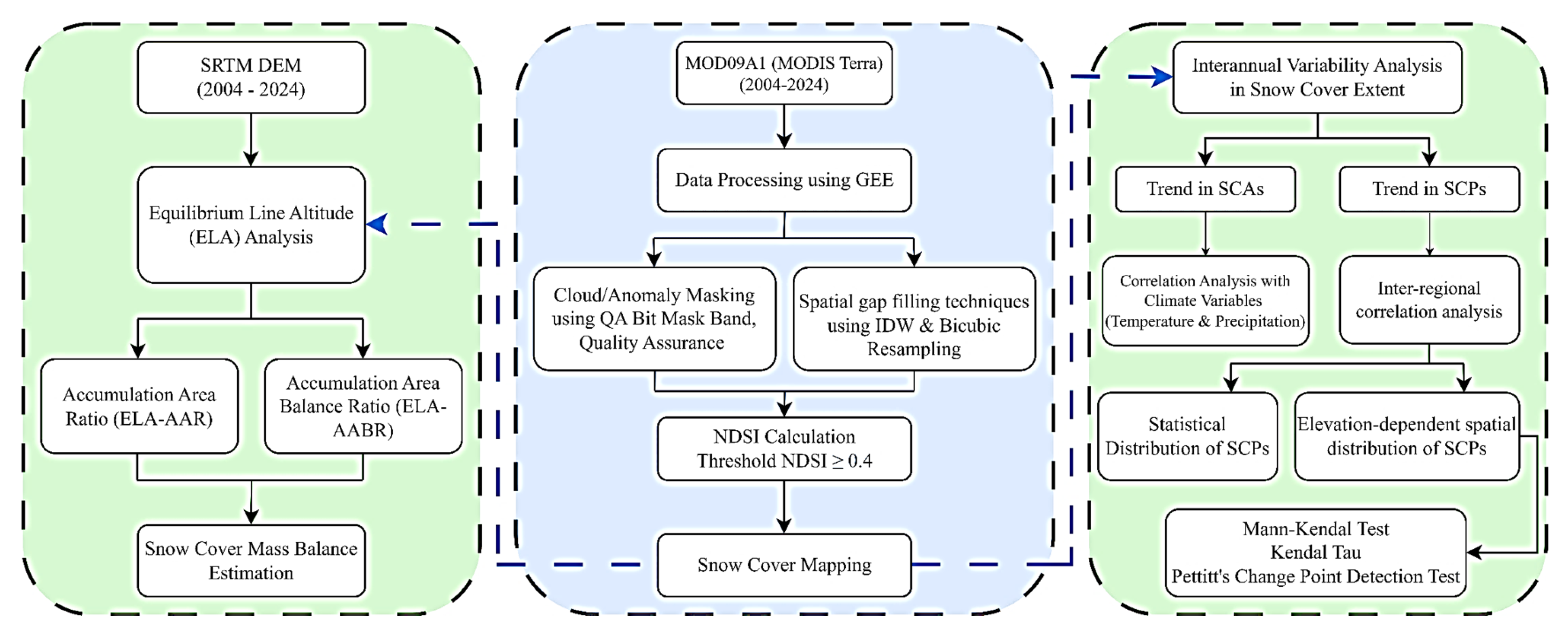
This study uses the MOD09A1 dataset, an 8-day composite surface reflectance product from the MODIS sensor. For each winter season (DJFM: December, January, February, and March) from 2004 to 2024, ~16 MOD09A1 composites per year were processed in Google Earth Engine (GEE) and averaged to create a seasonal mean mosaic per year (n = 21). The analysis followed a structured methodological framework within GEE, incorporating advanced spectral filtering, snow detection thresholding (NDSI ≥ 0.4), and gap-filling techniques, including Inverse Distance Weighting (IDW) and bi-cubic convolution. This workflow ensured reliable detection of snow cover across complex mountainous terrain (Figure 2).
Vector and raster geoprocessing workflows were automated using ArcPy in ArcGIS Pro (version 3.4.3). The ELA was calculated using the Python-based ELA Calculation Toolbox developed by Pellitero et al. [47], implemented as a custom ArcGIS tool. Trend and change-point analyses, including the Mann-Kendall test and Pettitt’s test, were performed using the pyMannKendall package (version 1.4.3) in Python (version 3.10.9). Kendall’s τ correlation coefficient was calculated using the SciPy library (version 1.10.0).

2.3.1. Data Preprocessing

To mitigate spectral anomalies caused by atmospheric interference, such as clouds, shadows, and water bodies, the MOD09A1 dataset was preprocessed using atmospheric filtration techniques based on a quality assurance (QA) bitmask band. Cloud-covered, shadowed, and water pixels were filtered by applying bitwise filtering procedures in GEE [37,48]. By systematically excluding flagged pixels, the dataset’s suitability for snow cover analysis during the snow season was significantly improved.
Missing values generated from the masking process were reconstructed using a bi-cubic convolution approach. Initially, masked pixels were restored with an unmasking function in GEE, followed by focal smoothing, using a 1.5 m-unit circular kernel to reduce local anomalies while preserving spatial details [49]. Pixel values were then interpolated using cubic polynomials, producing smoother and higher-quality results compared to linear methods. Finally, the interpolated reflectance values were standardized using a scaling factor of 0.0001 to match the radiometric scale of MOD09A1.

2.3.2. Snow Cover Pixels Detection

Snow-covered pixels (SCPs) were identified using the Normalized Difference Snow Index (NDSI), a well-established matrix that utilizes MODIS Green (Band 4) and SWIR1 (Band 6) reflectance. The NDSI was computed using the formula in Equation (1):
N D S I = G r e e n s u r _ r e f l _ b 04 S W I R 1 s u r _ r e f l _ b 06 G r e e n s u r _ r e f l _ b 04 + S W I R 1 s u r _ r e f l _ b 06 ,
A threshold value of NDSI ≥ 0.4, proven effective for distinguishing stable snow and glaciers, as well as other land surfaces [50,51], was applied to classify snow-covered pixels. This threshold is consistent with the MODIS global snow-mapping standard and validated through a sensitivity analysis by testing thresholds between 0.35 and 0.50. To further enhance the accuracy, the NDSI results were normalized using the Z-score method, improving overall comparability and enhancing the visual coherence of the snow cover dataset. The classified NDSI images were then employed to delineate SCAs, and their interannual variability was quantified using the annual rate of change (ROC).
Additionally, the SCAs were correlated with monthly averaged 2-m air temperature and total precipitation from the ERA5 reanalysis dataset for 2004–2024. ERA5 grids overlapping the Western, Central, and Eastern Himalayas were spatially aggregated using zonal statistics to derive regional monthly means for the winter season (DJFM). These temperature and precipitation series were compared with MODIS-derived SCAs to evaluate the influence of climatic variability on snow cover dynamics across the study period.

2.3.3. SCPs Variability Analysis

Three statistical approaches, i.e., (i) Mann–Kendall (MK) test, (ii) Kendall’s τ, and (iii) Pettitt’s test (for the change point detection), were used to analyze the variability in winter snow cover from 2004 to 2024. These methods were specifically chosen for their ability to detect trends, measure associations, and identify significant shifts in snow cover patterns. Together, they form a more robust and reliable framework for assessing snow cover variability by capturing both gradual changes and sudden transitions in snow dynamics. This integrated approach offers deeper insights into snow accumulation and melting behaviors over time, aligning with the research objective of evaluating long-term snow cover dynamics.
(i)
Mann–Kendall (MK) Test
The Mann–Kendall (MK) test was used to detect monotonic trends in snow cover variability, specifically snow accumulation or reduction, over the study period. The MK test statistic S was calculated as below:
S   =   k = 1 n 1 j = k + 1 n s g n ( X j X k ) ,
where the   s g n function s g n X j X k is defined as follows:
s g n X j X k =   i f   X j X k > 0 ,             1 i f   X j X k = 0 ,             0 i f   X j X k < 0 ,       1 ,
Here, X j and X k are the data values at times j and k, respectively, and n is the length of the dataset. The standardized test statistic ZS was then computed:
Z S = S 1 v a r s                                 i f   S > 0 0                                                     i f   S = 0 S + 1 v a r ( S )                           i f   S < 0 ,
The significance of the trend was evaluated by comparing ZS to critical values corresponding to specific confidence levels. Trends were considered statistically significant at 99%, 95%, and 90% confidence levels if ZS > 2.56, ZS > 1.96, and ZS > 1.65, respectively. If ZS exceeded these thresholds, the null hypothesis of no trend was rejected. Positive ZS values indicate increasing snow cover trends, while negative values indicate decreasing trends in snow cover.
(ii)
Kendall’s τ
Kendall’s τ test was used to evaluate the strength and direction of the relationship between time and changes in snow cover [52]. In combination with the MK test, it ensures a more comprehensive understanding of the temporal patterns in snow cover variability. The Kendall’s τ is defined in Equation (5):
τ   =   2 S n ( n   1 ) ,
where S represents the sum of the ranks of the differences between all pairs of observations, and n is the total number of observations in the time series. The value of S accounts for the relative ordering of paired observations, making it particularly effective for datasets with non-linear trends or fluctuations.
The sign of τ indicates the direction of the trend; a positive τ suggests an increasing trend in snow cover, whereas a negative τ indicates a decreasing trend over time. This makes the Kendall’s τ test especially suitable for analyzing snow cover variability in regions characterized by non-uniform temporal patterns.
(iii)
Pettitt’s Test (for change point detection)
Pettitt’s test (for change point detection) was used to identify abrupt shifts within the time-series data. In the analysis of snow cover variability, this test was employed to identify critical transition points in the snow cover time series, providing insights regarding abrupt changes in snow patterns or melting dynamics. The test statistic U t , n is defined in Equation (6):
U t , n =   i = 1 t j = t + 1 n s g n ( X i X j ) ,
where
s g n X i X j = i f   X i X j > 0 ,             1 i f   X i X j = 0 ,             0 i f   X i X j < 0 ,     1
The change point in the snow cover time series is identified at the point where Ut,n reaches its maximum value, denoted as KT, as shown in Equation (8):
KT = max Ut,n,
A decreasing trend in Ut over time suggests the presence of an abrupt change, whereas an increasing trend implies no significant change. If the test statistic surpasses the p-value threshold (p ≤ 0.05), it confirms the existence of a statistically significant change point detected in the dataset [53].

2.3.4. Snow Mass Balance Estimation Using ELA-Based AAR and AABR Methods

The hypsometrically controlled Accumulation Area Ratio (AAR) and Area-Altitude Balance Ratio (AABR) methods were used to estimate the Equilibrium Line Altitude (ELA) for snow mass balance in the WH, CH, and EH, respectively. The ELA separates the accumulation zone (above ELA, where snow is retained) from the ablation zone (below ELA, where snow mass loss occurs) and was derived using composite NDSI imagery (2004–2024) combined with the SRTM DEM. The AAR method, originally proposed by Kurowski [54], estimates ELA based on the ratio of accumulation area to total SCA, as expressed in Equation (9):
A A R = A c c u m u l a t i o n   A r e a   ( A A ) T o t a l   S n o w   C o v e r   A r e a   ( S C A ) ,
Considering the rugged topography of the Himalayas, AAR ratios between 0.4 and 0.8 were tested at 0.05 intervals, with a standard reflectance value of 0.5, indicating an equal distribution between accumulation and ablation zones. The AABR method, following [55] and [56], estimates ELA by considering the ratio of accumulation and ablation rates across elevation bands, as given in Equation (10):
A A B R =   L o w e s t   e l e v a t i o n E L A A r e a   ×   A c c u m u l a t i o n   R a t e   d E E L A H i g h e s t   e l e v a t i o n A r e a   ×   A b l a t i o n   R a t e   d E ,
where E denotes elevation (m) and d E is the differential elevation increment (m).
This study employed AABR ratios between 0.9 and 4.4 at 0.01 intervals.
In this study, we used both AAR and AABR methods to cross-validate ELA estimates. While the AAR method is widely applied in glaciological research, the AABR method incorporates mass balance gradients and accounts for topographic asymmetry, providing more robust and reliable results. The dual-method approach has been validated in previous ELA estimation studies [47,57], particularly in regions with snow-fed glaciers and complex hypsometric distributions.
A sophisticated toolbox developed by Pellitero et al. [47] for ArcGIS, which integrates Python scripts, was used to automate the ELA calculation for the Himalayas. This tool processed multiple snow cover datasets and leveraged DEM data with 50 m contour intervals (±5 m error) to simplify ELA determination. The analysis was conducted for the WH, CH, and EH, recording AAR and AABR values of 0.67 and 1.75, respectively. The lowest standard deviation values for AAR (0.5) and AABR (0.6) were applied, indicating a steady state for SCAs and a consistent accumulation-to-ablation ratio. Globally, several studies have reported various AAR and AABR ratios for ELA estimation [58], demonstrating that mass balance is strongly influenced by the altitudinal area relative to the ELA.

2.3.5. Model Performance Evaluation

To evaluate the MOD09A1-derived NDSI classifications, we computed annual confusion metrics from 2004 to 2024. These metrics provide a comprehensive framework for evaluating the performance of a predictive model. The key parameters include
True Positives (TP): snow pixels correctly classified as snow;
False Positives (FP): non-snow pixels incorrectly classified as snow;
False Negatives (FN): snow pixels missed by the classifier; and
True Negatives (TN): non-snow pixels correctly classified as non-snow.
These metrics collectively contribute to various evaluation measures such as Overall Accuracy (OA), the proportion of correctly classified pixels, calculated as follows:
O A = T P + T N T P + T N + F P + F N ,
Precision, the fraction of predicted snow pixels that are truly snow (penalizing commission errors), is calculated as follows:
P r e c i s i o n   =   T P T P   +   F P ,
Overall accuracy reflects global correctness, while precision specifically addresses commission errors in the snow class.
Recall, the fraction of actual snow pixels correctly identified (penalizing omission errors), calculated as follows:
R e c a l l = T P T P   +   F N ,
F1 score, the harmonic mean of Precision and Recall, balancing omission and commission errors, computed as follows:
F 1 = 2 P r e c i s i o n     ×   R e c a l l P r e c i s i o n   +   R e c a l l ,
Misclassification rate (MR) is defined as the overall error rate, calculated as follows:
M R = 1     O A ,
Lastly, the Kappa statistic (Ka), calculated using Equation (15), was quantitatively essential for providing a detailed evaluation of pixel-to-pixel classification accuracy. This approach considers the possibility of random agreement between predicted and observed classifications, thereby offering a rigorous assessment of the model’s effectiveness in spatial classification [59].
K a = S C o S C p 1 S C p ,
where SCo is the proportion of observed agreement, S C o   = ( T P   +   T N ) N while SCp is the proportion of expected (chance) agreement derived from the confusion-matrix marginals.

3. Results

3.1. Snow Cover Validation

The NDSI-based snow classification results derived from MOD09A1 were validated against the reference MODIS Terra Snow Cover product (MOD10A1F). The results exhibited a strong model fit and high-performance confidence, with an average Kappa coefficient (Ka) of 0.9129. The Overall Accuracy (OA) averaged 0.99, while the Misclassification Rate (MR) remained low (≈0.01), further confirming the robustness and reliability of the classifier. Detailed annual values for Ka, OA, Precision, Recall, F1 score, and MR are summarized in Table 1.

3.2. Interannual Variability in SCAs

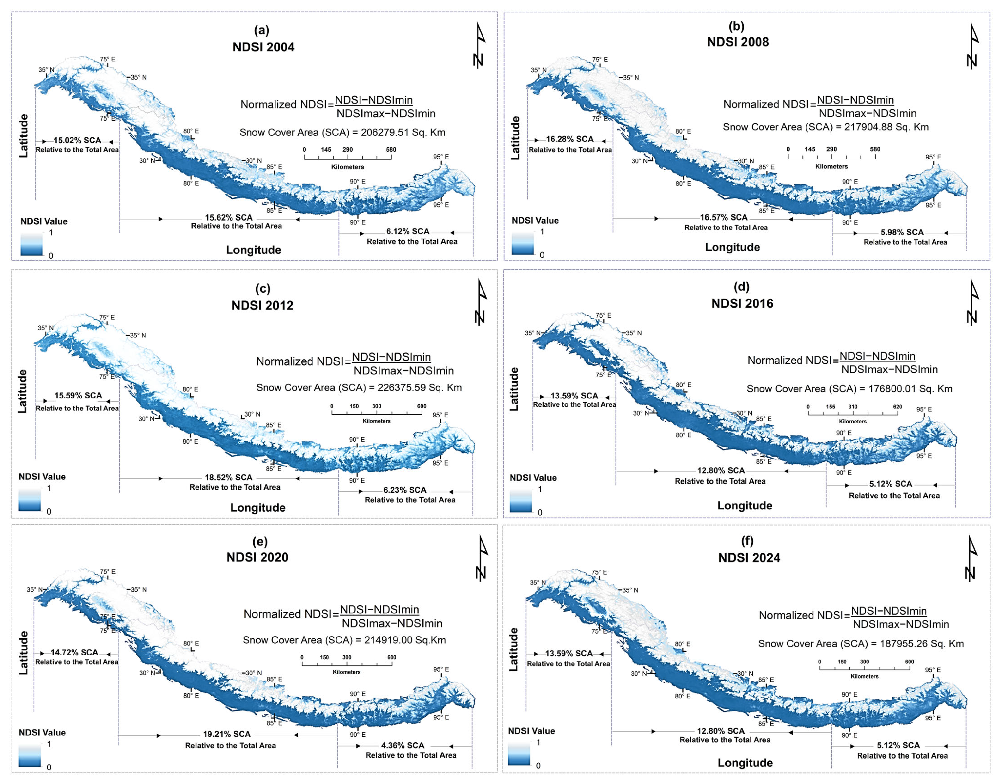
Figure 3 and Table S1 provide a comprehensive analysis of SCAs across the entire Himalayas from 2004 to 2024. Over this period, the mean SCA was 2.10 × 10⁵ km2, with a pronounced peak of 2.55 × 10⁵ km2 in 2019 and a low of 1.68 × 10⁵ km2 in 2021. The interannual Coefficient of Variation (CV) of 11.4% reflected moderate year-to-year fluctuations around this mean. These results show substantial annual variability but no marked long-term trend in overall snow cover.
Sub-regional variability indicates that the CH holds the largest share of snow cover (45.2%), followed by the WH (40.65%) and EH (14.15%), respectively (Figure 4). This trend suggests substantial regional disparities, with the CH having the most extensive snow cover. It also exhibits a higher proportion of transient snow, which makes it potentially more vulnerable to climatic shifts.
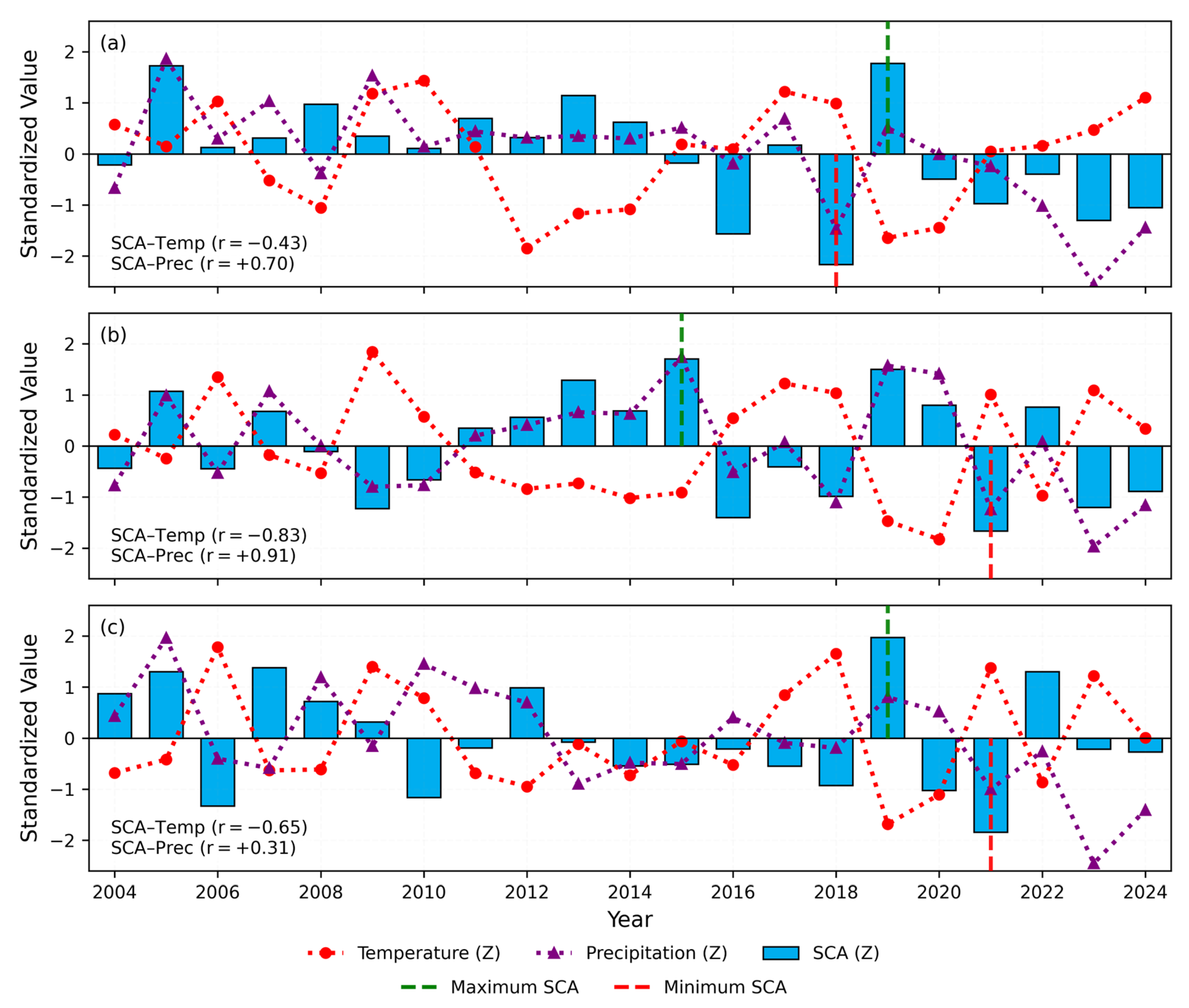
In detail, the WH recorded an average SCA of 8.59 × 10⁴ km2, with a maximum snow cover recorded in 2019 at 9.61 × 10⁴ km2, which exceeded the average by 1.28 × 10⁴ km2. A declining trend in SCA was observed between 2019 and 2023; however, this trend was statistically non-significant, indicating no consistent long-term changes in this region. The SCA varied between 7.26 × 10⁴ km2 and 9.61 × 10⁴ km2, with the highest positive mass balance observed between 2018 and 2019 at a rate of +32.31%. This gain was primarily driven by a sharp temperature drop of about 1.92 °C (−6.78 °C to −8.71 °C) and a concurrent rise in precipitation of +179.6 mm (from 264.3 mm to 443.9 mm), both favoring enhanced snow accumulation. Conversely, the most substantial negative mass balance occurred between 2017 and 2018, with a rate of change of −16.12%, correlating with a significant decrease in precipitation of about −195.9 mm (460.2 mm to 264.3 mm). Pearson correlation analysis confirms that SCA in WH is strongly influenced by precipitation (r = + 0.70, p < 0.001), predominantly associated with Western Disturbances (WDs), whereas the temperature showed a moderate and negative relation with SCA (r = −0.43, p ≈ 0.05), shown in Figure 5. The variability within the SCAs was quantified using the Coefficient of Variation (CV), which was calculated at 6.97%. The CV indicates a low degree of variability in SCAs and suggests a relatively stable snow cover pattern for this region.
The average SCA recorded in the CH was ~9.55 × 10⁴ km2, with major peaks observed in 2005 (11.22 × 10⁴ km2), 2013 (11.57 × 10⁴ km2), 2015 (12.26 × 10⁴ km2), and 2019 (11.93 × 10⁴ km2), respectively. Among these, 2015 marked the absolute maximum, exceeding the average by +2.71 × 10⁴ km2, mainly driven by relatively low temperatures (−2.99 °C) and high precipitation (394.2 mm). In contrast, 2009, 2016, 2018, 2021, and 2023 experienced relatively low SCAs, with 2021 marking the minimum at 6.76 × 10⁴ km2, about −2.79 × 10⁴ km2 below the average, associated with warmer and drier climate conditions (−1.17 °C temperature; 173.7 mm precipitation). The highest positive percentage gain in SCA was recorded between 2021 and 2022 (+58.46%), driven by a cooling of ~1.88 °C (from −1.17 °C to −3.05 °C) and an increase in precipitation of +98.0 mm (from 173.7 mm to 271.7 mm). Conversely, the period between 2015 and 2016 showed a substantial negative mass balance (−41.37%), caused by a warming of +1.38 °C and a sharp precipitation decline of −166.9 mm. The SCA in the CH exhibits a strong positive correlation with precipitation (r = +0.91, p < 0.0001) and a strong negative correlation with temperature (r = −0.83, p < 0.001), as shown in Figure 5. This highlights the region’s high sensitivity to climatic variability, primarily driven by WDs, Indian Summer Monsoon (ISM), and steep topography, which together make the CH snow cover highly sensitive to short-term climatic fluctuations. The mean CV for the CH was noted at 17.24%, indicating a moderate but notable variability in SCAs.
In the EH, significant increases in snow cover extent were recorded in 2005 (3.63 × 10⁴ km2), 2007 (3.72 × 10⁴ km2), 2019 (4.01 × 10⁴ km2), and 2022 (3.66 × 10⁴ km2), resulting in an average SCA of ~2.99 × 10⁴ km2 from 2004 to 2024. The maximum SCA was observed in 2019, exceeding the average by +1.34 × 10⁴ km2, attributed to colder temperatures (−0.34 °C) and relatively high precipitation (600.6 mm). In contrast, 2006, 2016, 2021, and 2023 recorded relatively low SCAs, with 2021 marking the lowest at 2.02 × 10⁴ km2, nearly −0.97 × 10⁴ km2 below the average, linked to warmer and drier conditions (+1.91 °C temperature; 413.3 mm precipitation). The largest absolute SCA gains occurred during 2021–22 (+80.8%; −1.65 °C, +77.1 mm) and 2018–19 (+60.5%; −2.25 °C, +108.4 mm). Conversely, the period from 2019 to 2020 recorded the highest negative rate of change at −38.9%%, when the snow cover declined by ~1.56 × 10⁴ km2, indicating a significant mass loss. This decline was primarily attributed to warming temperature (+0.43 °C) and reduced precipitation (−29.1 mm). In the EH, SCA is strongly and negatively correlated with temperature (r = −0.65, p ≈ 0.001) and weakly correlated with precipitation (r = +0.31, p ≈ 0.17) (Figure 5). This indicates that warming-driven reductions in winter snow cover are dominant, largely caused by rain–snow phase shifts, resulting in a higher snowline, and earlier rain-on-snow events that accelerate melting in this region. The mean CV for the EH was 17.45%, underscoring significant variability in snow extent from 2004 to 2024.

3.3. Temporal Variability of Snow Cover at Pixel Scale

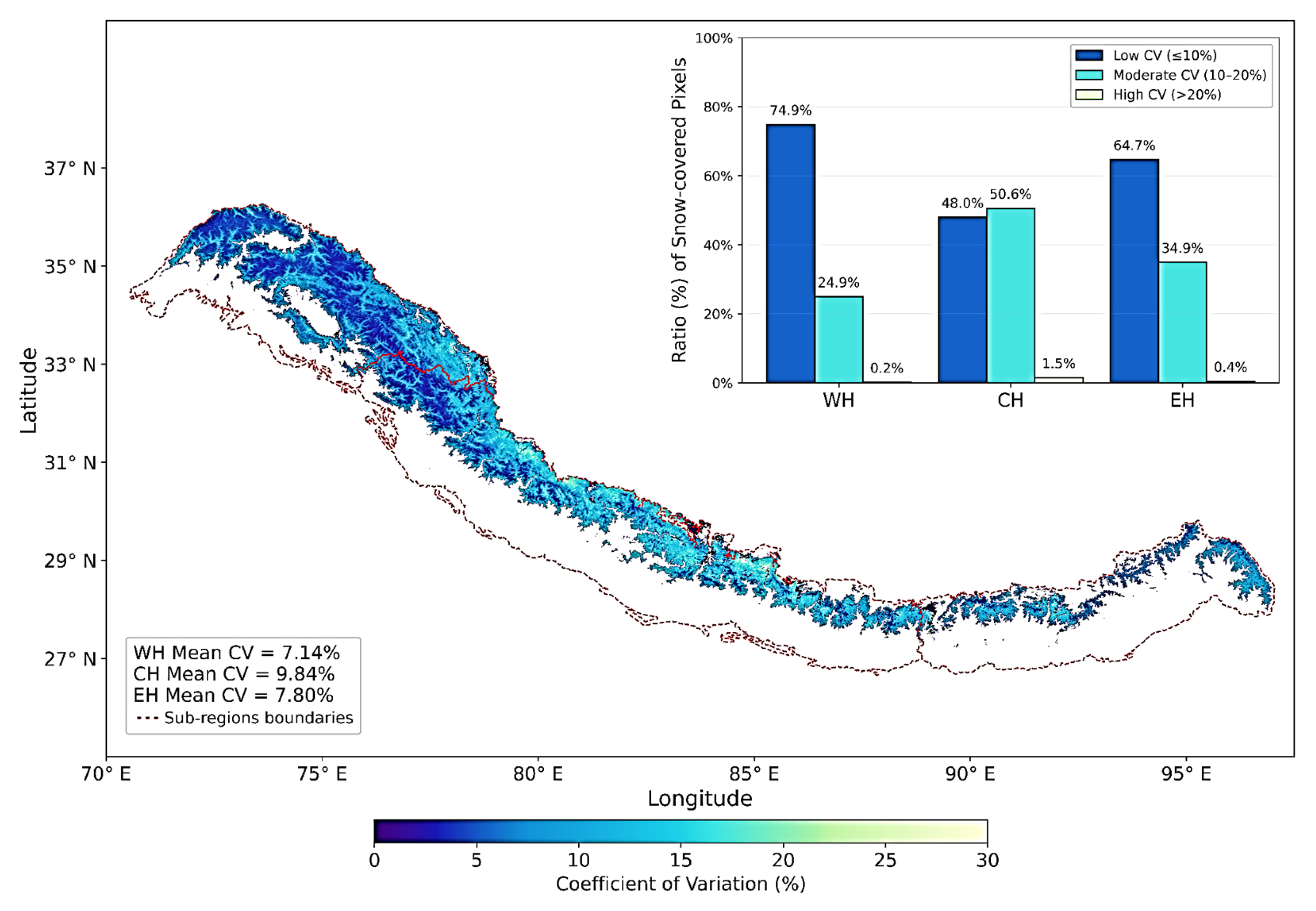
The interannual variability of snow cover at the pixel scale was quantified using the CV of the NDSI time series. As shown in Figure 6, there is relatively low variability across all regions, with mean CV values of 7.14% in the WH, 9.84% in the CH, and 7.80% in the EH, indicating overall stability. Approximately 70% of SCPs exhibit low variability, with the majority located in the WH (74.9%), followed by the EH (64.7%) and the CH (48.0%). Moderate variability is more prevalent in the CH, where 50.6% of SCPs show moderate variation in snow cover extent. In comparison, the WH and EH exhibit only 24.9% and 34.9% of SCPs with moderate variability, respectively. The proportion of high-variability pixels remains minimal across all regions, with only 0.2% in the WH, 1.5% in the CH, and 0.4% in the EH. This indicates limited significant changes in snow cover variability over the study period (2004–2024). Overall, these results demonstrate that Himalayan snow cover has remained largely stable over the past two decades. Among all regions, only the CH shows a modestly higher tendency toward moderate variability, whereas high variability remains notably low across all SCPs.
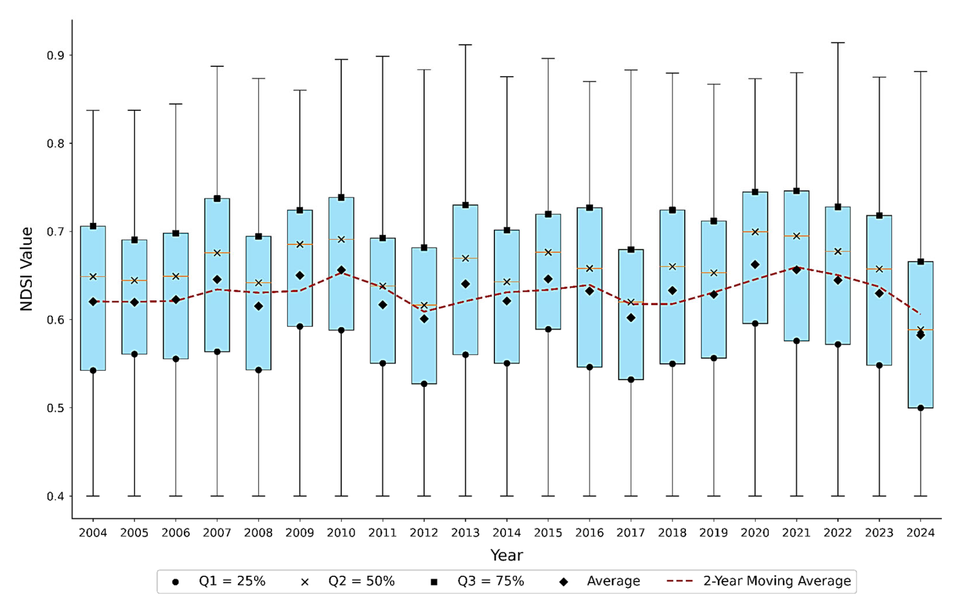
This pixel-based stability is further confirmed by the distribution of NDSI values (≥ 0.4) across the Himalayas (2004–2024), as shown in Figure 7. The mean NDSI fluctuated between 0.55 and 0.75, suggesting a relatively stable central tendency. Higher interquartile ranges (IQRs) in 2010 and 2018 indicated significant variability in those years, whereas smaller IQRs in 2015 and 2024 reflected more consistent snow cover with less variability. The linear regression analysis of annual mean NDSI values reveals a marginal upward trend (y = 0.0001x + 0.6289), with a slight increase in snow cover over time (2004–2024).

3.4. Elevation-Dependent Spatial Distribution of the SCPs Across the Himalayas

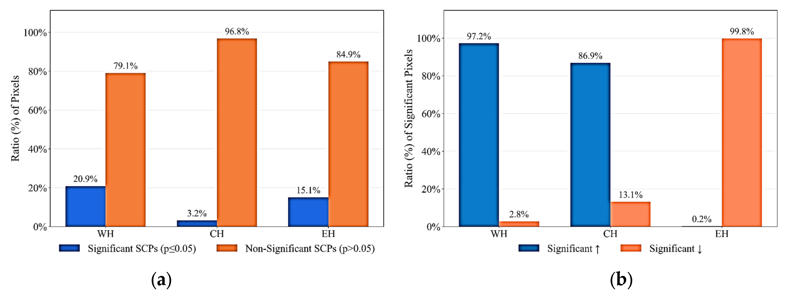
The trend analysis, using the Mann-Kendall (MK) test, reveals that ~30% of the SCPs across the Himalayas exhibited statistically significant trends (p ≤ 0.05), as shown in Figure 8. These trends indicate spatially heterogeneous patterns of snow accumulation and ablation during 2004 to 2024. Most of these significant changes were concentrated at higher elevations. In contrast, the remaining 70% of SCPs showed no statistically significant trends (p > 0.05), suggesting a stable winter snow cover across much of the region.
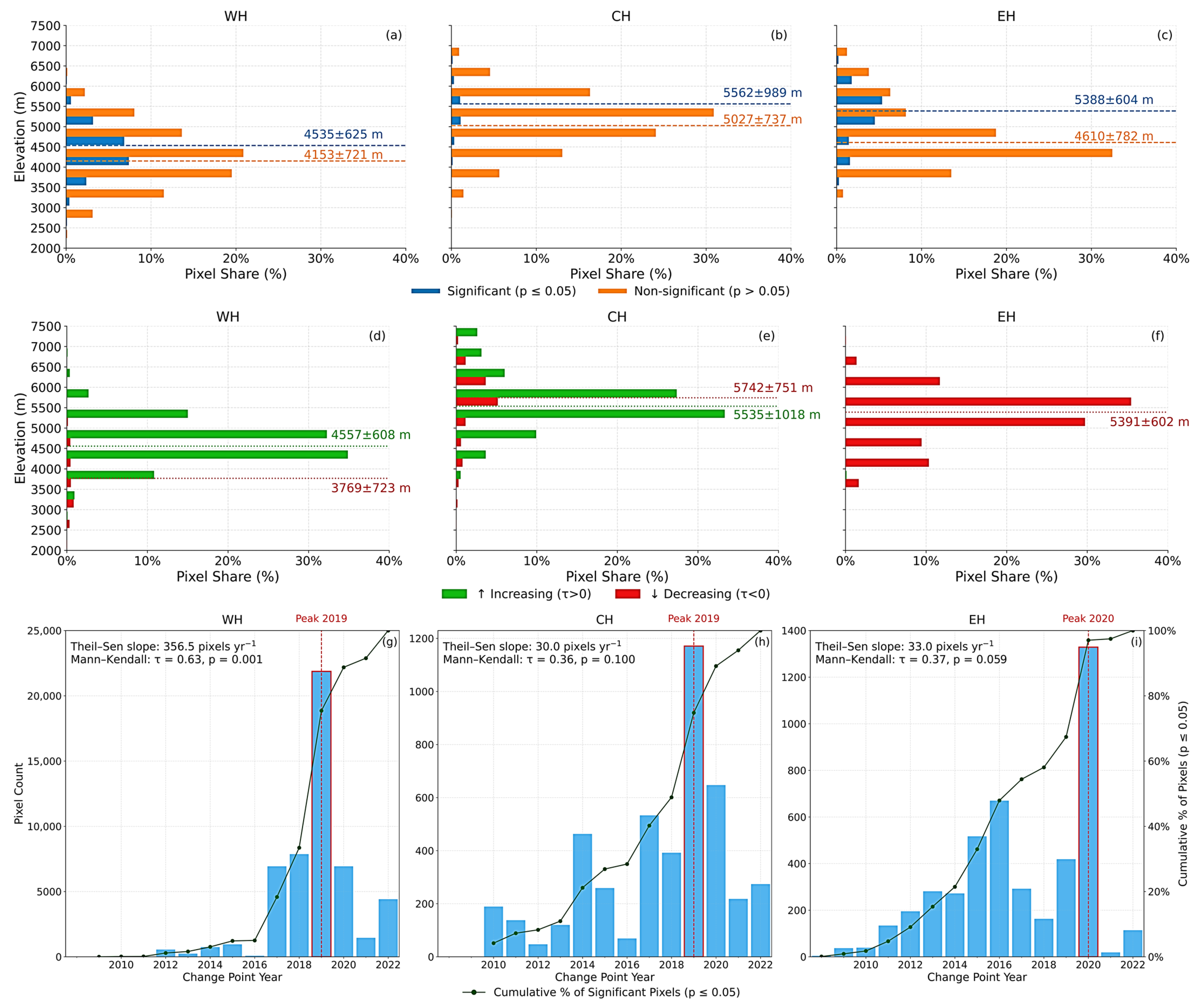
Within the WH, ~21% of SCPs (≈65,109 pixels) exhibited statistically significant trends (p ≤ 0.05), mostly concentrated in slightly higher-altitude zones. These regions include the Zanskar Range (Ladakh, Northwestern India), Pir Panjal range (Jammu and Kashmir, Northwestern India), and Northern Pakistan, with a mean elevation of 4528.90 ± 536.91 m. In contrast, non-significant trends (p > 0.05) were more broadly distributed across mid-altitude zones, with a mean elevation of 4151.29 ± 699.47 m (Figure 9a). Kendall’s τ analysis indicated that ~97% of significantly changed pixels in WH exhibited increasing trends, concentrated at marginally higher altitudes around 4516.12 ± 531.94 m. In comparison, only 3% showed decreasing trends, mainly across lower to mid-elevation areas (3797.82 ± 725.37 m) (Figure 9b). Between 2008 and 2022, the annual pixel count with statistically significant change-points increased steadily, reaching a Theil–Sen slope of +356 pixels yr−1. Significant change-points were detected in 2016 (decline) and 2019 (increase), followed by a resurgence of increasing snow cover post-2021 (Figure 9c). Together, these results indicate an overall positive mass balance, with increasing snow cover across the WH during the study period.
In the CH, only 3% of SCPs exhibited statistically significant trends (p ≤ 0.05), predominantly situated in high-altitude zones (5525.14 ± 704.69 m). In contrast, non-significant trends, comprising ~97% of SCPs, were primarily distributed across mid-altitude zones (5019.42 ± 674.50 m) (Figure 9d). Of the significant pixels, ~86.9% exhibited increasing trends, centered around 5487.34 ± 701.33 m, located in the Nanda Devi Range (Garhwal Himalaya, Uttarkhand, Northern India). While ~13.1% showed decreasing trends, located within the Kumaon Himalayas (Uttarkhand, Northern India), at slightly higher elevations (5781.01 ± 681.81 m) (Figure 9e). Between 2008 and 2022, change-point counts in the CH reached a Theil–Sen slope of +30 pixels yr−1, indicating only moderate statistical support for a long-term increase. Pettitt’s test detects an early surge in 2008–2009, a downturn in 2014–2015, a brief recovery around 2018, and then a downward phase. By 2019, the cumulative curve reaches roughly 75% of all significant pixels, pinpointing the late 2010s as the critical interval for CH snow-cover change (Figure 9f).
In the EH, ~15% of SCPs exhibited statistically significant trends (p ≤ 0.05) primarily concentrated at high elevation zones (5404.72 ± 612.41 m), compared to non-significant pixels, which were common at mid-elevations (4579.15 ± 734.90 m) (Figure 9g). Notably, all statistically significant pixels in the EH exhibited decreasing trends, mainly located within the Kanchenjunga region (Northeastern India and Eastern Nepal), Tongshanjiabu (Bhutan-Tibet border, Northern Bhutan), Kangkar Punzum (Bhutan-China border, Northern Bhutan), Kula Kangri (China), and Arunachal Pradesh (Northeastern India), centered around a mean elevation of 5408.02 ± 608.48 m (Figure 9h). In the EH, significant change-point pixels reach a Theil–Sen rate of +33 pixels yr−1, between 2008 and 2022. Pettitt’s test identifies two key breakpoints in 2014 and 2018, both corresponding to intervals of snow loss, with 2020 marking the peak year of change (Figure 9i). However, the overall linear trend in snow cover itself is negative, pointing to a gradual decline in EH snow extent over the twenty-one-year period.

3.5. Snow Cover Mass Balance Estimation Based on AAR and AABR

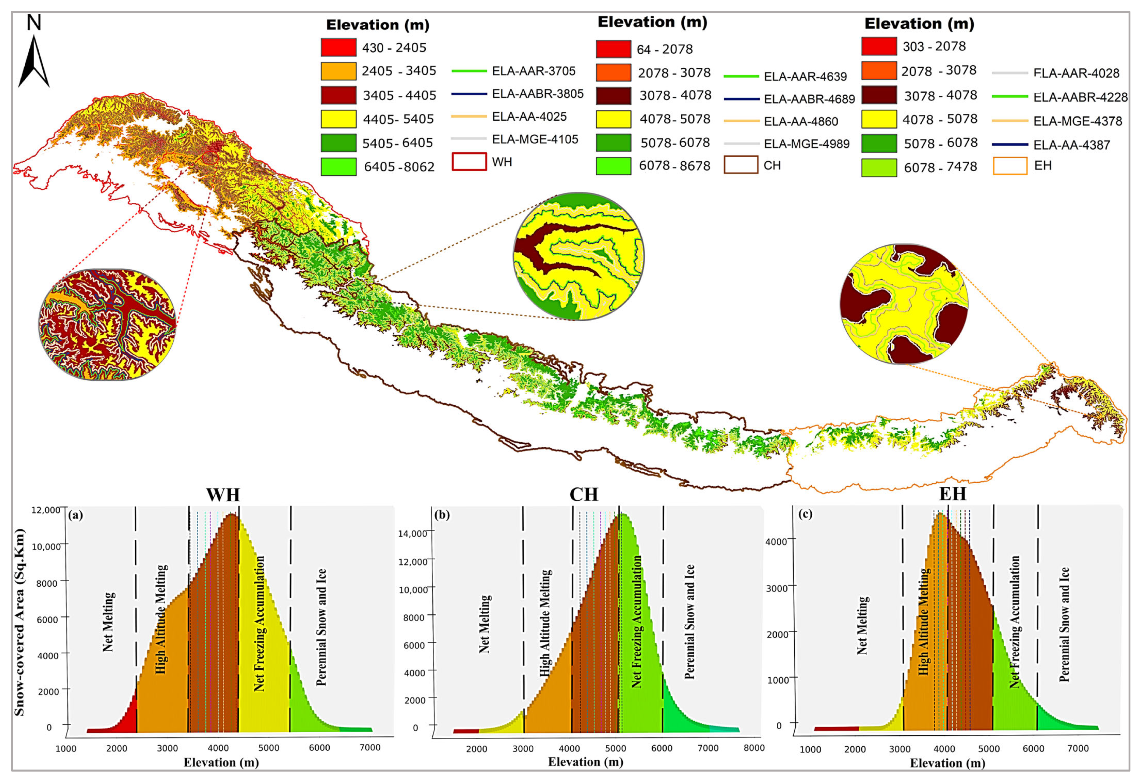
SCAs in the WH followed a quasi-normal distribution, peaking between 3855 m and 4605 m with the highest concentration of 33.93%. The distribution tapers sharply toward both extremes (0.58% below 2155 m; 1.14% above 5855 m), highlighting sharp declines at both extremes (Figure 10a). Nearly 81.08% of SCAs occupy the mid-elevation range (3155–5150 m), where the hypsometric curve exhibited a gradual slope (relatively flat), indicating a central tendency around these altitudes with stable snow retention. At an AAR of 0.67, 64.48% of the total SCPs lie in the steeper regions < 3705 m, representing the ablation zone, while the remaining 35.52% constitutes the accumulation zone. Whereas, for an AABR of 0.96, the ablation zone expanded to 60.77%, while the accumulation zone reduced to 39.23%, extending up to 3805 m. This reflects the dominant role of mid-altitude terrain in governing WH snow cover dynamics and the vulnerability of extreme elevations to snow loss.
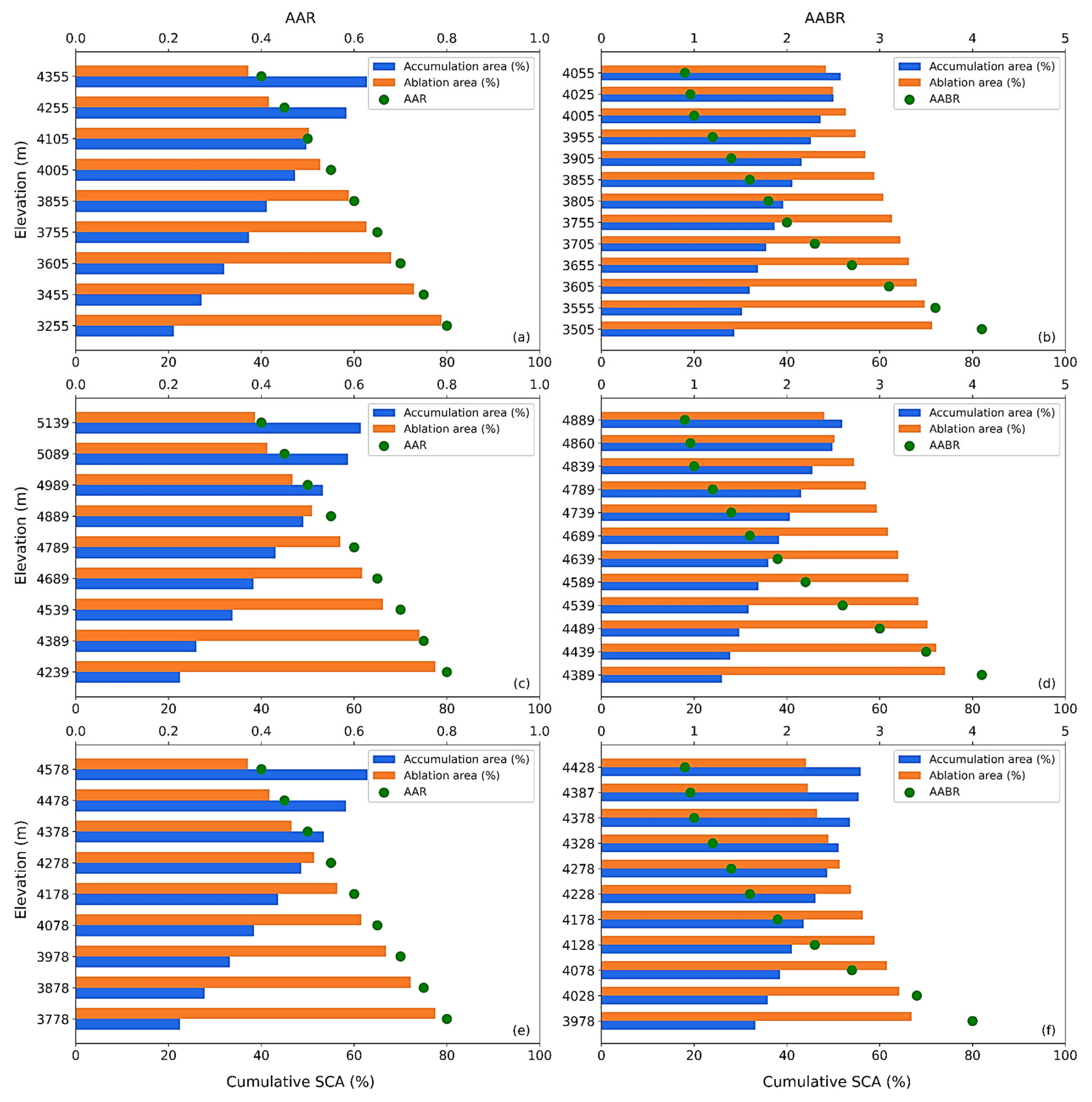
Variations in SCA geometries of WH, based on AAR and AABR-ELA ratios, are summarized in Figure 11a,b and detailed in Table S2. At an AAR of 0.5 and ELA of 4105 m, 48.37% of the area lies in the ablation zone (<4105 m), while 51.63% is in the accumulation zone (>4105 m). For an AABR of 0.96, the ablation area comes out to be 51.42%, and the accumulation 48.58%, located at an ELA of 4025 m. Raising AAR from 0.4 to 0.8 lowered the ELA by 1100 m, from 4355 m to 3255 m, corresponding to a 41.64% reduction in the accumulation area. Similarly, increasing the AABR from 0.9 to 4.4 lowered the ELA by 550 m, from 4055 m to 3505 m, resulting in a 20.47% gain in the ablation area. When maintaining a constant AAR between 0.4 and 0.45, a 100 m ELA decrease from 4355 m to 4255 m led to a 4.44% reduction in SCA. The most significant decrease, 200 m, was observed for a constant AAR of 0.75 to 0.8, resulting in a 5.98% loss in snow cover geometries. The losses in SCAs were highly variable, with the highest positive mass balance occurring between elevations (3855–4005 m). In contrast, a relatively low degree of positive mass balance was reported between elevations of 3755 m and 3855 m for varying AAR values.
Snow cover in the CH exhibits a normal distribution, peaking between 4389 m and 5589 m, with the highest concentration (59.66%) of SCAs (Figure 10b). Snow coverage tapers at extremes, with only 1.38% found at higher elevations (6489 m and 8739 m), and 1.04% at lower elevations < 2889 m, representing a skew toward mid-altitudinal ranges. A significant portion (84.67%) of SCAs was concentrated between 3739 m and 5889 m, where the hypsometric curve exhibited a steep slope. Almost 64% of the total SCA was concentrated in steeper regions > 4989 m, corresponding to the accumulation zone, while the remaining 36% occupied the ablation zone, based on an AAR of 0.67. When applying an AABR of 0.96, the distribution shifted, with the accumulation zone expanding to 53.03% and the ablation zone decreasing to 46.97%, extending up to an elevation of 4860 m. This indicates a redistribution of snow cover across the elevation gradient, reflecting changes in the snow accumulation and ablation dynamics of CH.
ELA analysis (Figure 11c,d; Table S3) confirms that positive mass balance was concentrated in the steeper portion of the curve > 4989 m. At this elevation, 53.05% of the area lies in the accumulation zone and 46.98% in the ablation zone, based on an AAR of 0.5. In comparison, at an AABR of 0.96 (ELA of 4860 m), the accumulation area constitutes 50.48% while the ablation area of 49.42% relative to the total SCA. Raising AAR from 0.4 to 0.8 lowered the ELA by 900 m, from 5139 m to 4239 m, corresponding to an approximate 38.89% reduction in the ablation area. Moreover, increasing the AABR from 0.9 to 4.4 reduced the ELA by 500 m, from 4889 m to 3889 m, resulting in a ~22.09% decrease in the accumulation area. A 100 m decrease in ELA, from 5089 m to 4989 m, resulted in a 5.39% reduction in SCA while maintaining a constant AAR between 0.45 and 0.5. The most significant degree of negative mass balance, a 150 m drop in ELA, was observed with a constant AAR of 0.7 to 0.75, leading to a 7.87% loss in snow cover geometries. The lowest negative mass balance was concentrated between the elevations of 5139 m and 5089 m, resulting in a 2.72% reduction in area, indicating a zone for mass loss.
Snow cover in the EH showed a slightly positive skewed distribution (Figure 10c), with the majority (49.88%) of SCA concentrated between elevations of 3628 m and 4528 m. Snow cover falls off sharply toward the extremes, with only 0.15% of the snow found at higher elevations (7028–7478 m) and 0.21% at lower elevations (<2728 m). This underscores a strong mid-elevation focus. Almost 92.77% of SCAs lie between 3328 m and 5678 m, where the hypsometric curve showed a steep gradient. Approximately 64% of the total SCA was located in the steeper regions >4028 m, corresponding to the ablation zone. The remaining 35.82% lies in the accumulation zone, as defined by an AAR of 0.67. Applying an AABR of 0.96 shifts the equilibrium to 4228 m, expanding the ablation zone to 53.84% and reducing the accumulation zone to 46.15%. This indicates a notable upward redistribution of snow cover.
ELA analysis for the EH (Figure 11e,f and Table S4) indicated a positive mass balance, predominantly concentrated in the steeper section of the curve, centered at>4378 m. At this elevation, 53.52% of the SCA is in the accumulation zone, while 46.48% in the ablation zone, at an AAR of 0.5. Conversely, for an AABR of 0.96, the mass balance at 4387 m comprised 55.47% of the accumulation area and 44.53% of the ablation area relative to the total SCA. Raising AAR from 0.4 to 0.8 lowers the ELA by 800 m, from 4578 m to 3778 m, corresponding to an approximate 40.41% reduction in the accumulation area. Similarly, elevating the AABR from 0.9 to 4.4 decreased the ELA by 450 m, from 4428 m to 3978 m, leading to an approximate 22.75% reduction in the accumulation area. A 100 m decrease in ELA, from 4478 m to 4378 m, resulted in a 4.76% reduction in the SCA when the AAR was held constant between 0.45 and 0.5. The most pronounced negative mass balance was observed with a constant AAR between 0.55 and 0.6, where a 100 m drop in ELA led to a 6.18% loss in snow cover geometries. The lowest negative mass balance was concentrated between elevations of 4378 m, resulting in a 3.71% reduction in area, marking a critical zone of mass loss.

4. Discussion

This study applied a pixel-based methodology to analyze snow cover variability across the Himalayan region. The results demonstrate the effectiveness of advanced spectral filtering and gap-filling techniques. The spectral filtration approach specifically targeted spectral anomalies such as cloud cover, shadows, and water bodies [60,61,62]. By systematically excluding non-snow pixels, this process significantly enhanced the reliability of snow cover mapping, ensuring that the analysis focused solely on high-confidence snow pixels. To manage data, bi-cubic convolution interpolation was employed, effectively addressing masked pixels. This method maintained spatial continuity and mitigated common interpolation errors like voids and spectral confusion. Validation against the MOD10A1F snow cover product, which has ~93% accuracy under clear-sky conditions [27], highlighted the robustness of the applied methodology. The validation achieved an overall accuracy of 99.02%, with a precision of 87.67%, a recall of 96.36%, an F1 score of 91.81%, and a Kappa statistic of 0.9129, demonstrating the strong performance of the algorithm across diverse Himalayan terrains and climatic conditions. Moreover, owing to the sensor-independent and scalable design of the adopted methodology, it is methodologically adaptable to other mountainous regions, such as the European Alps and the Andes. However, the application may require minor region-specific adjustments (e.g., canopy-aware indices in forested regions and fractional snow mapping in patchy snow environments).

4.1. Variations in Snow Cover Trends Across Different Regions of the Himalayas

This study identified region-specific trends in snow cover across the Himalayan range. In the WH, there is a significant increasing trend in SCAs, with maximum concentrations occurring at higher altitudes (4516.12 ± 531.94 m). These results align closely with previous studies by [63] and [64]. These results are further supported by an increasing frequency and magnitude of Western-Induced Precipitation, the Indian Ocean Dipole, and cloudburst events, all of which positively influence the snow mass balance in this region [63,64,65,66,67]. The IPCC Fifth Assessment Report (AR5) similarly indicated positive SCA trends for the WH due to increased precipitation [68]. Additionally, recent studies have observed slight shifts in the Western Disturbances linked to the westerly jet stream during winter, shifting precipitation patterns toward the pre-monsoon season. This supports the observed positive anomaly in snow cover for the WH [69,70,71].
Conversely, the CH experienced significant reductions in SCA during 2016 and 2021. In 2016, SCA decreased by 41.37% due to warmer and drier conditions (+1.38 °C temperature, −166.9 mm precipitation). While in 2021, the SCA declined by ~29.2%, reaching the absolute minimum of 6.76 × 10⁴ km2 under similar conditions (−1.17 °C, 173.7 mm). Previous studies reinforce this temperature sensitivity, indicating that years with increased SCAs typically coincide with lower temperatures [72,73]. Our findings corroborate existing literature, highlighting an insignificant decreasing trend in snow cover at lower elevations. In contrast, a slightly significant increasing trend is observed at higher altitudes due to less exposure of these elevations to solar radiation and persistently freezing conditions throughout the year [67,74,75,76,77].
In the EH, a significant decreasing trend in SCA was marked by a notable decline in snow extent. This reduction is attributed primarily to the subtropical climate conditions prevalent in the region, characterized by shorter winters, delayed snow onset, and early snowmelt processes [78,79]. These findings also align with research documenting reductions in SCA at higher elevations, particularly during winter months. This decline is attributed to rising air and surface temperatures, indicative of shifting climatic patterns within this region [65,80].

4.2. Climatic Influences and Spatial Variability

The dynamic snow cover trends observed across the Western, Central, and Eastern Himalayas highlight significant climatic and spatial variability within the region. This variability is driven by the vast east-west extent of the Himalayan range and diverse local and regional atmospheric processes. Specifically, the climate of the WH is strongly influenced by Western-induced precipitation patterns, closely resembling that of the southern Karakoram region. As a result, the WH exhibits comparable snow cover characteristics, similar to those observed in Shigar [65]. In contrast to the global glacier melting trends driven by climate warming, certain valleys in the Karakoram and WH show localized positive snow cover trends. This phenomenon is commonly referred to as the Karakoram anomaly [70,81,82]. Moreover, recent temperature increases in regions such as the Pamir Mountains and Tibetan Plateau have further enhanced the moisture transfer and deep convection processes. These changes influence snow cover variability within the Himalayan foothills [65].

4.3. Snow Mass Balance and ELA

The evaluation of positive and negative mass balances indicated the ELA for the EH at an altitude of 4378 m, corresponding to an AAR of 0.5, yielding a negative mass balance of −0.015. Similarly, a slightly higher altitude ELA of 4989 m was recorded for the CH, associated with a negative net mass balance (−0.0268). These negative balances correlate with significant temperature variability and warming trends observed within these regions [83,84]. Conversely, the WH exhibited a positive mass balance (0.0389), strongly correlating with regional topographical and temperature variability across the Himalayas. Lin et al. [85] documented mass gains of 0.043 ± 0.078 to 0.363 ± 0.065 m between 2011 and 2014 in west Kunlun, eastern Pamir, and northern Karakoram, while western Karakorum exhibited a near-stable balance of −0.020 ± 0.064 m. The Upper Tarim Basin in Karakorum also exhibited a positive mass balance, with a decreasing gradient from northeast to southwest [85]. These contrasting mass-balance trends are primarily controlled by regional climatic regimes. The positive mass balance in the WH is driven by enhanced winter precipitation from WDs. In contrast, negative trends in the CH and EH, dominated by monsoonal influence, are mainly attributed to elevation-dependent warming, resulting in accelerated snow retreat at higher elevations [86]. While traditional applications of ELA-AAR and AABR techniques primarily focus on glacier mass balances [87,88], our approach uniquely emphasizes snow cover balance, utilizing both constant and variable ratios. Cross-validation of the AAR (0.5) and AABR (0.67) ratios, with variable AAR (0.4–0.8) and AABR (0.9–4.4), reduced methodological uncertainty by ∼33%. This thereby enhances the reliability of our results and provides comprehensive insights into Himalayan snow cover dynamics.

5. Conclusions

This study provides a comprehensive assessment of snow cover variability across the Himalayas from 2004 to 2024. Advanced spectral filtering and gap-filling techniques were applied to mitigate anomalies caused by cloud cover and shadows. The use of a circular kernel method with bi-cubic convolution preserved spatial continuity and effectively addressed data gaps. The model’s robustness was validated against the MOD10A1F dataset, achieving strong performance metrics, including a Kappa coefficient of 0.9129, an Overall Accuracy of 99.02%, and an F1 score of 91.81%. High Recall and Precision values further confirm the reliability of this approach for regional snow cover mapping and highlight its value for hydrological and environmental monitoring.
Two key findings emerge from the analysis. First, a significant increase in snow cover was observed at higher elevations, particularly around 4516 m. Regional variability is evident, with the WH exhibiting increasing snow cover trends, driven mainly by winter precipitation, whereas the EH demonstrates declining trends primarily attributed to warming temperatures. This contrast highlights the interactions between global atmospheric processes and localized climatic factors across the Himalaya’s extensive east-west gradient. This variability emphasizes the complexity inherent in Himalayan climate systems. Second, the mass balance analysis using the ELA–AAR and AABR methods revealed distinct regional differences. The WH shows a positive mass balance, while the Central and Eastern Himalayas display negative balances. These findings align with the recognized “Karakoram anomaly”, where localized glacier growth occurs in specific parts of the WH and Karakoram, despite the broader global trend of glacier retreat. This variability emphasizes the crucial role of localized climatic drivers in shaping snow dynamics across mountainous regions.
Overall, this study highlights the importance of assessing spatial and temporal snow cover variability across the Himalayas. It provides valuable insights for climate impact analysis, water resource management, and ecosystem sustainability in this ecologically vulnerable region. By integrating cloud-corrected MODIS data, spectral indices, statistical models, and elevation-based metrics (e.g., ELA-based AAR and AABR), the research addresses key spatial and methodological gaps. The findings support informed decision-making for water management, climate adaptation, and hazard preparedness, emphasizing the need for continued monitoring and long-term assessment in the Himalayas.

Supplementary Materials

The following supporting information can be downloaded at: https://www.mdpi.com/article/10.3390/rs17183175/s1, Table S1: Regional share of SCAs (%) in Himalayas from 2004 to 2024 relative to total extent; Table S2: AAR-AABR ratios for SCAs of WH; Table S3: AAR-AABR ratios for SCAs of CH; Table S4: AAR-AABR ratios for SCAs of EH.

Author Contributions

Conceptualization, G.T. and W.Z.; methodology, G.T. and W.Z.; software, G.T. and M.X.; validation, G.T. and M.X.; formal analysis, G.T. and W.Z.; investigation, G.T. and W.Z.; data curation, G.T. and W.Z.; writing—original draft preparation, G.T.; writing—review and editing, G.T., W.Z. and D.F.; visualization, G.T. and M.X.; supervision, W.Z.; project administration, W.Z.; funding acquisition, W.Z. All authors have read and agreed to the published version of the manuscript.

Funding

This research was jointly supported by the National Natural Science Foundation of China (42222109), the Science and Technology Program of the Tibet Autonomous Region (XZ202401ZY0060), the Key Program of the Chinese Academy of Sciences for International Cooperation (162GJHZ2023065MI), and the Science and Technology Research Program of the Institute of Mountain Hazards and Environment (IMHE-CXTD-02).

Data Availability Statement

The MODIS/Terra surface reflectance product (MOD09A1, v6.1) used in this study is publicly available from the NASA Land Processes Distributed Active Archive Center (LP DAAC) at https://doi.org/10.5067/MODIS/MOD09A1.061 (accessed on 30 December 2023). The MODIS/Terra daily snow-cover product (MOD10A1F, v6.1) is freely accessible from the NASA National Snow and Ice Data Center (NSIDC) Distributed Active Archive Center at https://doi.org/10.5067/MODIS/MOD10A1F.061 (accessed on 7 January 2024). The Shuttle Radar Topography Mission (SRTM) 30 m Digital Elevation Model (DEM) data were obtained from the U.S. Geological Survey’s EarthExplorer portal: https://earthexplorer.usgs.gov (accessed on 12 July 2024). The ERA5 monthly averaged reanalysis dataset providing 2 m air temperature and total precipitation was downloaded from the Copernicus Climate Data Store (CDS) at https://cds.climate.copernicus.eu (accessed on 27 August 2025). The Elevation-Line-Altitude (ELA) analysis was performed using the ELA-calculation toolbox for ArcGIS 10.1 (and later versions) developed by Pellitero et al. [47], available at https://github.com/cageo/Pellitero-2015 (accessed on 17 July 2024). The algorithm for reconstructing filtered snow-cover data and any additional code or processed datasets are available from the authors upon reasonable request.

Conflicts of Interest

The authors declare no conflicts of interest.

Abbreviations

The following abbreviations are used in this manuscript:
AAArea-Altitude
AABRAccumulation-Area Balance Ratio
AARAccumulation Area Ratio
CGFCloud-gap-filled
CHCentral Himalayas
DJFMDecember, January, February, March
EDWElevation-dependent warming
EHEastern Himalayas
ELAEquilibrium Line Altitude
FNFalse Negatives
FPFalse Positives
GEEGoogle Earth Engine
HMAHigh Mountain Asia
IDWInverse Distance Weighting
IQRsInterquartile ranges
ISMIndian Summer Monsoon
MGEMedian Glacier Elevation
MKMann-Kendall test
MODISModerate Resolution Imaging Spectroradiometer
MRMisclassification rate
KaKappa statistic
CVCoefficient of Variation
NDSI Normalized Difference Snow Index
OAOverall Accuracy
QAQuality Assurance
SCASnow-covered Area
SCE Snow cover extent
SCPsSnow-covered Pixels
SRTMShuttle Radar Topography Mission
TNTrue Negatives (TN)
TPTrue Positives
WDsWestern Disturbances
WH Western Himalayas

References

  1. Immerzeel, W.W.; van Beek, L.P.H.; Konz, M.; Shrestha, A.B.; Bierkens, M.F.P. Hydrological response to climate change in a glacierized catchment in the Himalayas. Clim. Change 2012, 110, 721–736. [Google Scholar] [CrossRef]
  2. Bolch, T.; Kulkarni, A.; Kääb, A.; Huggel, C.; Paul, F.; Cogley, J.G.; Frey, H.; Kargel, J.S.; Fujita, K.; Scheel, M.; et al. The State and Fate of Himalayan Glaciers. Science 2012, 336, 310–314. [Google Scholar] [CrossRef]
  3. Bookhagen, B.; Burbank, D.W. Toward a complete Himalayan hydrological budget: Spatiotemporal distribution of snowmelt and rainfall and their impact on river discharge. J. Geophys. Res. Earth Surf. 2010, 115, F03019. [Google Scholar] [CrossRef]
  4. Hock, R.; Rasul, G.; Adler, C.; Cáceres, B.; Gruber, S.; Hirabayashi, Y.; Jackson, M.; Kääb, A.; Kang, S.; Kutuzov, S. High mountain areas. In IPCC Special Report on the Ocean and Cryosphere in a Changing Climate; Pörtner, H.-O., Roberts, D.C., Masson-Delmotte, V., Zhai, P., Tignor, M., Poloczanska, E., Mintenbeck, K., Alegría, A., Nicolai, M., Okem, A., et al., Eds.; IPCC: Geneva, Switzerland, 2019; pp. 131–202. [Google Scholar]
  5. Xiao, L.; Che, T.; Chen, L.; Xie, H.; Dai, L. Quantifying snow albedo radiative forcing and its feedback during 2003–2016. Remote Sens. 2017, 9, 883. [Google Scholar] [CrossRef]
  6. Li, Y.; Tao, H.; Su, B.; Kundzewicz, Z.W.; Jiang, T. Impacts of 1.5 °C and 2 °C global warming on winter snow depth in Central Asia. Sci. Total Environ. 2019, 651, 2866–2873. [Google Scholar]
  7. Sankey, T.; Donald, J.; McVay, J.; Ashley, M.; O’Donnell, F.; Lopez, S.M.; Springer, A. Multi-scale analysis of snow dynamics at the southern margin of the North American continental snow distribution. Remote Sens. Environ. 2015, 169, 307–319. [Google Scholar] [CrossRef]
  8. Banerjee, A.; Chen, R.; Meadows, M.E.; Sengupta, D.; Pathak, S.; Xia, Z.; Mal, S. Tracking 21st century climate dynamics of the Third Pole: An analysis of topo-climate impacts on snow cover in the central Himalaya using Google Earth Engine. Int. J. Appl. Earth Obs. Geoinf. 2021, 103, 102490. [Google Scholar]
  9. Frei, A.; Robinson, D.A. Northern Hemisphere snow extent: Regional variability 1972–1994. Int. J. Climatol. 1999, 19, 1535–1560. [Google Scholar] [CrossRef]
  10. Joshi, R.; Tamang, N.D.; Balraju, W.; Singh, S.P. Spatial and seasonal patterns of temperature lapse rate along elevation transects leading to treelines in different climate regimes of the Himalaya. Biodivers. Conserv. 2024, 33, 3517–3538. [Google Scholar] [CrossRef]
  11. Kattel, D.B.; Yao, T.; Yang, K.; Tian, L.; Yang, G.; Joswiak, D. Temperature lapse rate in complex mountain terrain on the southern slope of the central Himalayas. Theor. Appl. Climatol. 2013, 113, 671–682. [Google Scholar] [CrossRef]
  12. Sabin, T.P.; Krishnan, R.; Vellore, R.; Priya, P.; Borgaonkar, H.P.; Singh, B.B.; Sagar, A. Climate Change Over the Himalayas. In Assessment of Climate Change over the Indian Region: A Report of the Ministry of Earth Sciences (MoES), Government of India; Krishnan, R., Sanjay, J., Gnanaseelan, C., Mujumdar, M., Kulkarni, A., Chakraborty, S., Eds.; Springer: Singapore, 2020; pp. 207–222. [Google Scholar] [CrossRef]
  13. Shen, L.; Zhang, Y.; Ullah, S.; Pepin, N.; Ma, Q. Changes in snow depth under elevation-dependent warming over the Tibetan Plateau. Atmos. Sci. Lett. 2021, 22, e1041. [Google Scholar] [CrossRef]
  14. Wester, P.; Chaudhary, S.; Maharjan, A.; Steiner, J.F.; Chettri, N.; Chettri, R.; Jackson, M.; Nepal, S.; Wang, X. Water, Ice, Society, and Ecosystems in the Hindu Kush Himalaya: An Introduction; International Centre for Integrated Mountain Development (ICIMOD): Khumaltar, Nepal, 2023; pp. 1–15. [Google Scholar]
  15. Mukhtar, H.; Yang, Y.; Xu, M.; Wu, J.; Abbas, S.; Wei, D.; Zhao, W. Elevation-Dependent Vegetation Greening and Its Responses to Climate Changes in the South Slope of the Himalayas. Geophys. Res. Lett. 2025, 52, e2024GL113276. [Google Scholar] [CrossRef]
  16. Notarnicola, C. Overall negative trends for snow cover extent and duration in global mountain regions over 1982–2020. Sci. Rep. 2022, 12, 13731. [Google Scholar] [CrossRef]
  17. Fugazza, D.; Manara, V.; Senese, A.; Diolaiuti, G.; Maugeri, M. Snow cover variability in the greater alpine region in the MODIS era (2000–2019). Remote Sens. 2021, 13, 2945. [Google Scholar] [CrossRef]
  18. Rohrer, M.; Salzmann, N.; Kulkarni, A. Missing (in-situ) snow cover data hampers climate change and runoff studies in the Greater Himalayas. Sci. Total Environ. 2013, 468, S60–S70. [Google Scholar] [CrossRef] [PubMed]
  19. Lievens, H.; Demuzere, M.; Marshall, H.P.; Reichle, R.H.; Brucker, L.; Brangers, I.; de Rosnay, P.; Dumont, M.; Girotto, M.; Immerzeel, W.W.; et al. Snow depth variability in the Northern Hemisphere mountains observed from space. Nat. Commun. 2019, 10, 4629. [Google Scholar] [CrossRef] [PubMed]
  20. Gao, S.; Zeng, J.; Li, Z.; Letu, H.; Zhang, P.; Huang, L.; Qiao, H.; Chen, Q. Measuring global snow water equivalent from passive microwave remote sensing: Opportunities and challenges. Innov. Geosci. 2024, 2, 100062. [Google Scholar] [CrossRef]
  21. Hammond, J.C.; Saavedra, F.A.; Kampf, S.K. Global snow zone maps and trends in snow persistence 2001–2016. Int. J. Climatol. 2018, 38, 4369–4383. [Google Scholar] [CrossRef]
  22. Notarnicola, C. Hotspots of snow cover changes in global mountain regions over 2000–2018. Remote Sens. Environ. 2020, 243, 111781. [Google Scholar] [CrossRef]
  23. Huang, Y.; Song, Z.; Yang, H.; Yu, B.; Liu, H.; Che, T.; Chen, J.; Wu, J.; Shu, S.; Peng, X.; et al. Snow cover detection in mid-latitude mountainous and polar regions using nighttime light data. Remote Sens. Environ. 2022, 268, 112766. [Google Scholar] [CrossRef]
  24. Hall, D.K.; Riggs, G.A.; DiGirolamo, N.E.; Román, M.O. Evaluation of MODIS and VIIRS cloud-gap-filled snow-cover products for production of an Earth science data record. Hydrol. Earth Syst. Sci. 2019, 23, 5227–5241. [Google Scholar] [CrossRef]
  25. Gascoin, S.; Hagolle, O.; Huc, M.; Jarlan, L.; Dejoux, J.F.; Szczypta, C.; Marti, R.; Sánchez, R. A snow cover climatology for the Pyrenees from MODIS snow products. Hydrol. Earth Syst. Sci. 2015, 19, 2337–2351. [Google Scholar] [CrossRef]
  26. Xu, N.; Li, W.; Gong, P.; Lu, H. Satellite altimeter observed surface water increase across lake-rich regions of the Arctic. Innovation 2024, 5, 100714. [Google Scholar] [CrossRef] [PubMed]
  27. Hall, D.K.; Riggs, G.A.; DiGirolamo, N.E.; Román, M.O. MODIS cloud-gap filled snow-cover products: Advantages and uncertainties. Hydrol. Earth Syst. Sci. Discuss. 2019, 123, 1–23. [Google Scholar]
  28. Li, Y.; Chen, Y. The continuing shrinkage of snow cover in High Mountain Asia over the last four decades. In Proceedings of the EGU General Assembly Conference Abstracts, Vienna, Austria, 24–28 April 2023; p. EGU-16661. [Google Scholar]
  29. Desinayak, N.; Prasad, A.K.; El Askary, H.; Kafatos, M.; Asrar, G.R. Snow cover variability and trend over the Hindu Kush Himalayan region using MODIS and SRTM data. Ann. Geophys. 2022, 40, 67–82. [Google Scholar] [CrossRef]
  30. Rikiishi, K.; Nakasato, H. Height dependence of the tendency for reduction in seasonal snow cover in the Himalaya and the Tibetan Plateau region, 1966–2001. Ann. Glaciol. 2006, 43, 369–377. [Google Scholar] [CrossRef]
  31. IPCC. Impacts, Adaptation and Vulnerability; Cambridge University Press: Cambridge, UK, 2007; p. 828. [Google Scholar]
  32. Khali, H.; Pandey, P.; Ali, S.N.; Champatiray, P.K. MODIS Observed Spatiotemporal Variation of Snow Cover in Zanskar Valley, North-Western Himalaya. Front. Water 2022, 4, 853146. [Google Scholar] [CrossRef]
  33. Mishra, B.; Babel, M.S.; Tripathi, N.K. Analysis of climatic variability and snow cover in the Kaligandaki River Basin, Himalaya, Nepal. Theor. Appl. Climatol. 2014, 116, 681–694. [Google Scholar] [CrossRef]
  34. Mishra, B.; Tripathi, N.K.; Babel, M.S. An artificial neural network-based snow cover predictive modeling in the higher Himalayas. J. Mt. Sci. 2014, 11, 825–837. [Google Scholar] [CrossRef]
  35. Moazzam, M.F.U.; Rahman, G.; Lee, B.G.; Ansari, N.A. Trend of snow cover under the influence of climate change using Google Earth Engine platform: A case study of Astore (Western Himalayas) and Shigar (Karakoram region). Front. Environ. Sci. 2022, 10, 1006399. [Google Scholar] [CrossRef]
  36. Hall, D.K.; Riggs, G.A. Accuracy assessment of the MODIS snow products. Hydrol. Process. 2007, 21, 1534–1547. [Google Scholar] [CrossRef]
  37. Chen, H.; Yong, B.; Qi, W.; Wu, H.; Ren, L.; Hong, Y. Investigating the evaluation uncertainty for satellite precipitation estimates based on two different ground precipitation observation products. J. Hydrometeorol. 2020, 21, 2595–2606. [Google Scholar] [CrossRef]
  38. Luo, L.; Zhang, J.; Wang, H.; Chen, M.; Jiang, Q.; Yang, W.; Wang, F.; Zhang, J.; Swain, R.B.; Meadows, M.E.; et al. Innovations in science, technology, engineering, and policy (iSTEP) for addressing environmental issues towards sustainable development. Innov. Geosci. 2024, 2, 100087. [Google Scholar] [CrossRef]
  39. Yang, G.; Zha, D.; Cao, D.; Zhang, G. Time for a change: Rethinking the global renewable energy transition from the Sustainable Development Goals and the Paris Climate Agreement. Innovation 2024, 5, 100582. [Google Scholar] [CrossRef]
  40. Vermote, E. MODIS/Terra Surface Reflectance 8-Day L3 Global 500m SIN Grid, V061; National Snow and Ice Data Center: Boulder, CO, USA, 2021. [Google Scholar]
  41. USGS. Land Processes DAAC (LP DAAC). Available online: https://earthexplorer.usgs.gov/ (accessed on 12 July 2024).
  42. Patil, R.; Mohanty, B.; Liu, B.; Chandrashekaran, I.R.; Headey, S.J.; Williams, M.L.; Clements, C.S.; Ilyichova, O.; Doak, B.C.; Genissel, P.; et al. A ligand-induced structural change in fatty acid–binding protein 1 is associated with potentiation of peroxisome proliferator–activated receptor α agonists. J. Biol. Chem. 2019, 294, 3720–3734. [Google Scholar] [CrossRef]
  43. Riggs, G.; Hall, D. Continuity of MODIS and VIIRS Snow Cover Extent Data Products for Development of an Earth Science Data Record. Remote Sens. 2020, 12, 3781. [Google Scholar] [CrossRef]
  44. Copernicus Climate Change Service (C3S). ERA5: Fifth Generation of ECMWF Atmospheric Reanalyses of the Global Climate. Available online: https://cds.climate.copernicus.eu (accessed on 27 August 2025).
  45. Hersbach, H.; Bell, B.; Berrisford, P.; Hirahara, S.; Horányi, A.; Muñoz-Sabater, J.; Nicolas, J.; Peubey, C.; Radu, R.; Schepers, D.; et al. The ERA5 global reanalysis. Q. J. R. Meteorol. Soc. 2020, 146, 1999–2049. [Google Scholar] [CrossRef]
  46. NASA JPL. NASA Shuttle Radar Topography Mission Global 1 Arc Second. 2013. Available online: https://www.earthdata.nasa.gov/data/catalog/lpcloud-srtmgl1-003 (accessed on 12 July 2024).
  47. Pellitero, R.; Rea, B.R.; Spagnolo, M.; Bakke, J.; Hughes, P.; Ivy Ochs, S.; Lukas, S.; Ribolini, A. A GIS tool for automatic calculation of glacier equilibrium-line altitudes. Comput. Geosci. 2015, 82, 55–62. [Google Scholar] [CrossRef]
  48. Chi, M.; Plaza, A.; Benediktsson, J.A.; Sun, Z.; Shen, J.; Zhu, Y. Big data for remote sensing: Challenges and opportunities. Proc. IEEE 2016, 104, 2207–2219. [Google Scholar] [CrossRef]
  49. Mahale, G.; Mahale, H.; Parimi, R.B.; Nandy, S.K.; Bhattacharya, S. Hardware architecture of bi-cubic convolution interpolation for real-time image scaling. In Proceedings of the 2014 International Conference on Field-Programmable Technology (FPT), Shanghai, China, 10–12 December 2014; pp. 264–267. [Google Scholar]
  50. Parajka, J.; Blöschl, G. Validation of MODIS snow cover images over Austria. Hydrol. Earth Syst. Sci. 2006, 10, 679–689. [Google Scholar] [CrossRef]
  51. Cheng, Q.; Shen, H.; Zhang, L.; Li, P. Inpainting for remotely sensed images with a multichannel nonlocal total variation model. IEEE Trans. Geosci. Remote Sens. 2013, 52, 175–187. [Google Scholar] [CrossRef]
  52. Kendall, M.G. Rank Correlation Methods; Charles Griffin & Co., Ltd.: London, UK, 1948; p. 160. [Google Scholar]
  53. Pettitt, A.N. A Non-Parametric Approach to the Change-Point Problem. J. R. Stat. Soc. Ser. C Appl. Stat. 1979, 28, 126–135. [Google Scholar] [CrossRef]
  54. Kurowski, L. Die Höhe der Schneegrenze: Mit besonderer Berücksichtigung der Finsteraarhorn-Gruppe; Hlözel Ed.: Vienna, Austria, 1891; p. 160. [Google Scholar]
  55. Osmaston, H. Estimates of glacier equilibrium line altitudes by the Area×Altitude, the Area × Altitude Balance Ratio and the Area × Altitude Balance Index methods and their validation. Quat. Int. 2005, 138–139, 22–31. [Google Scholar] [CrossRef]
  56. Furbish, D.J.; Andrews, J.T. The use of hypsometry to indicate long-term stability and response of valley glaciers to changes in mass transfer. J. Glaciol. 1984, 30, 199–211. [Google Scholar] [CrossRef]
  57. Baig, S.U.; Muneeb, F. Adjustment of glacier geometries to future equilibrium line altitudes in the Shigar River Basin of Karakoram Range, Pakistan. SN Appl. Sci. 2021, 3, 482. [Google Scholar] [CrossRef]
  58. Kern, Z.; László, P. Size specific steady-state accumulation-area ratio: An improvement for equilibrium-line estimation of small palaeoglaciers. Quat. Sci. Rev. 2010, 29, 2781–2787. [Google Scholar] [CrossRef]
  59. Sim, J.; Wright, C.C. The kappa statistic in reliability studies: Use, interpretation, and sample size requirements. Phys. Ther. 2005, 85, 257–268. [Google Scholar] [CrossRef]
  60. Ackerman, S.A.; Strabala, K.I.; Menzel, W.P.; Frey, R.A.; Moeller, C.C.; Gumley, L.E. Discriminating clear sky from clouds with MODIS. J. Geophys. Res. Atmos. 1998, 103, 32141–32157. [Google Scholar] [CrossRef]
  61. Stillinger, T.; Roberts, D.A.; Collar, N.M.; Dozier, J. Cloud masking for Landsat 8 and MODIS Terra over snow-covered terrain: Error analysis and spectral similarity between snow and cloud. Water Resour. Res. 2019, 55, 6169–6184. [Google Scholar] [CrossRef]
  62. Liu, A.; Che, T.; Huang, X.; Dai, L.; Wang, J.; Deng, J. Effect of Cloud Mask on the Consistency of Snow Cover Products from MODIS and VIIRS. Remote Sens. 2022, 14, 6134. [Google Scholar] [CrossRef]
  63. Gurung, D.R.; Maharjan, S.B.; Shrestha, A.B.; Shrestha, M.S.; Bajracharya, S.R.; Murthy, M.S.R. Climate and topographic controls on snow cover dynamics in the Hindu Kush Himalaya. Int. J. Climatol. 2017, 37, 3873–3882. [Google Scholar] [CrossRef]
  64. Anjum, M.N.; Ding, Y.; Shangguan, D.; Liu, J.; Ahmad, I.; Ijaz, M.W.; Khan, M.I. Quantification of spatial temporal variability of snow cover and hydro-climatic variables based on multi-source remote sensing data in the Swat watershed, Hindukush Mountains, Pakistan. Meteor. Atmos. Phys. 2019, 131, 467–486. [Google Scholar] [CrossRef]
  65. Muhammad Tahir, K.; Yin, Y.; Wang, Y.; Babar, Z.A.; Yan, D. Impact assessment of orography on the extreme precipitation event of July 2010 over Pakistan: A numerical study: A numerical study. Adv. Meteorol. 2015, 2015, 510417. [Google Scholar] [CrossRef]
  66. Shafiq, M.u.; Ahmed, P.; Islam, Z.u.; Joshi, P.K.; Bhat, W.A. Snow cover area change and its relations with climatic variability in Kashmir Himalayas, India. Geocarto Int. 2019, 34, 688–702. [Google Scholar] [CrossRef]
  67. Tahir, A.A.; Adamowski, J.F.; Chevallier, P.; Haq, A.U.; Terzago, S. Comparative assessment of spatiotemporal snow cover changes and hydrological behavior of the Gilgit, Astore and Hunza River basins (Hindukush–Karakoram–Himalaya region, Pakistan). Meteorol. Atmos. Phys. 2016, 128, 793–811. [Google Scholar] [CrossRef]
  68. Stocker, T. Climate Change 2013 the Physical Science Basis: Working Group I Contribution to the Fifth Assessment Report of the Intergovernmental Panel on Climate Change; 110705799X; Cambridge University Press: Cambridge, UK; New York, NY, USA, 2014; p. 1535. [Google Scholar]
  69. Midhuna, T.M.; Kumar, P.; Dimri, A.P. A new Western Disturbance Index for the Indian winter monsoon. J. Earth Syst. Sci. 2020, 129, 59. [Google Scholar] [CrossRef]
  70. Dimri, A.P. Decoding the Karakoram anomaly. Sci. Total Environ. 2021, 788, 147864. [Google Scholar] [CrossRef]
  71. Dimri, A.P.; Niyogi, D.; Barros, A.P.; Ridley, J.; Mohanty, U.C.; Yasunari, T.; Sikka, D.R. Western Disturbances: A review. Rev. Geophys. 2015, 53, 225–246. [Google Scholar] [CrossRef]
  72. Dharpure, J.K.; Goswami, A.; Patel, A.; Kulkarni, A.V.; Snehmani. Assessment of snow cover variability and its sensitivity to hydrometeorological factors in the Karakoram and Himalayan region. Hydrol. Sci. J. 2021, 66, 2198–2215. [Google Scholar] [CrossRef]
  73. Choudhury, A.; Yadav, A.C.; Bonafoni, S. A Response of Snow Cover to the Climate in the Northwest Himalaya (NWH) Using Satellite Products. Remote Sens. 2021, 13, 655. [Google Scholar] [CrossRef]
  74. Qureshi, M.A.; Yi, C.; Xu, X.; Li, Y. Glacier status during the period 1973–2014 in the Hunza Basin, Western Karakoram. Quat. Int. 2017, 444, 125–136. [Google Scholar] [CrossRef]
  75. Ali, S.; Khan, G.; Hassan, W.; Qureshi, J.A.; Bano, I. Assessment of glacier status and its controlling parameters from 1990 to 2018 of Hunza Basin, Western Karakorum. Environ. Sci. Pollut. Res. 2021, 28, 63178–63190. [Google Scholar] [CrossRef] [PubMed]
  76. Saydi, M.; Ding, J.l. Impacts of topographic factors on regional snow cover characteristics. Water Sci. Eng. 2020, 13, 171–180. [Google Scholar] [CrossRef]
  77. Hasson, S.; Lucarini, V.; Pascale, S.; Böhner, J. Seasonality of the hydrological cycle in major South and Southeast Asian river basins as simulated by PCMDI/CMIP3 experiments. Earth Syst. Dyn. 2014, 5, 67–87. [Google Scholar] [CrossRef]
  78. Sharma, A.; Choudhury, M. Chapter 17—Changing climate and depleting water resources in the mountains with a case study from the Himalayas. In Water Conservation in the Era of Global Climate Change; Thokchom, B., Qiu, P., Singh, P., Iyer, P.K., Eds.; Elsevier: Amsterdam, The Netherlands, 2021; pp. 411–436. [Google Scholar]
  79. Negi, H.S.; Kumar, A.; Kanda, N.; Thakur, N.K.; Singh, K.K. Status of glaciers and climate change of East Karakoram in early twenty-first century. Sci. Total Environ. 2021, 753, 141914. [Google Scholar] [CrossRef]
  80. Krishnan, R.; Shrestha, A.B.; Ren, G.; Rajbhandari, R.; Saeed, S.; Sanjay, J.; Syed, M.A.; Vellore, R.; Xu, Y.; You, Q.; et al. Unravelling Climate Change in the Hindu Kush Himalaya: Rapid Warming in the Mountains and Increasing Extremes. In The Hindu Kush Himalaya Assessment: Mountains, Climate Change, Sustainability and People; Wester, P., Mishra, A., Mukherji, A., Shrestha, A.B., Eds.; Springer International Publishing: Cham, Switzerland, 2019; pp. 57–97. [Google Scholar]
  81. Hewitt, K. The Karakoram anomaly? Glacier expansion and the’elevation effect,’Karakoram Himalaya. Mt. Res. Dev. 2005, 25, 332–340. [Google Scholar] [CrossRef]
  82. Farinotti, D.; Immerzeel, W.W.; de Kok, R.J.; Quincey, D.J.; Dehecq, A. Manifestations and mechanisms of the Karakoram glacier Anomaly. Nat. Geosci. 2020, 13, 8–16. [Google Scholar] [CrossRef]
  83. Bolch, T.; Pieczonka, T.; Mukherjee, K.; Shea, J. Brief communication: Glaciers in the Hunza catchment (Karakoram) have been nearly in balance since the 1970s. Cryosphere 2017, 11, 531–539. [Google Scholar] [CrossRef]
  84. Maurer, J.M.; Schaefer, J.M.; Rupper, S.; Corley, A. Acceleration of ice loss across the Himalayas over the past 40 years. Sci. Adv. 2019, 5, eaav7266. [Google Scholar] [CrossRef]
  85. Lin, H.; Li, G.; Cuo, L.; Hooper, A.; Ye, Q. A decreasing glacier mass balance gradient from the edge of the Upper Tarim Basin to the Karakoram during 2000–2014. Sci. Rep. 2017, 7, 6712. [Google Scholar] [CrossRef]
  86. Kuttippurath, J.; Patel, V.K.; Sharma, B.R. Observed changes in the climate and snow dynamics of the Third Pole. npj Clim. Atmos. Sci. 2024, 7, 162. [Google Scholar] [CrossRef]
  87. Trueba, J.J.G.; Canadas, E.S. The AAR Method for Palaeo-ELA determination: Methodological analysis and application to Valdecebollas Massif (Cantabrian Range). Geophys. Res. Lett. 2004, 30, 7–34. [Google Scholar]
  88. Zasadni, J.; Świąder, A.; Kłapyta, P. A novel (raster input/output) method of equilibrium line altitude (AAR, AABR) estimation and glacier hypsometry analysis. In Proceedings of the EGU General Assembly Conference Abstracts, Vienna, Austria, 4–13 April 2018; p. 18556. [Google Scholar]
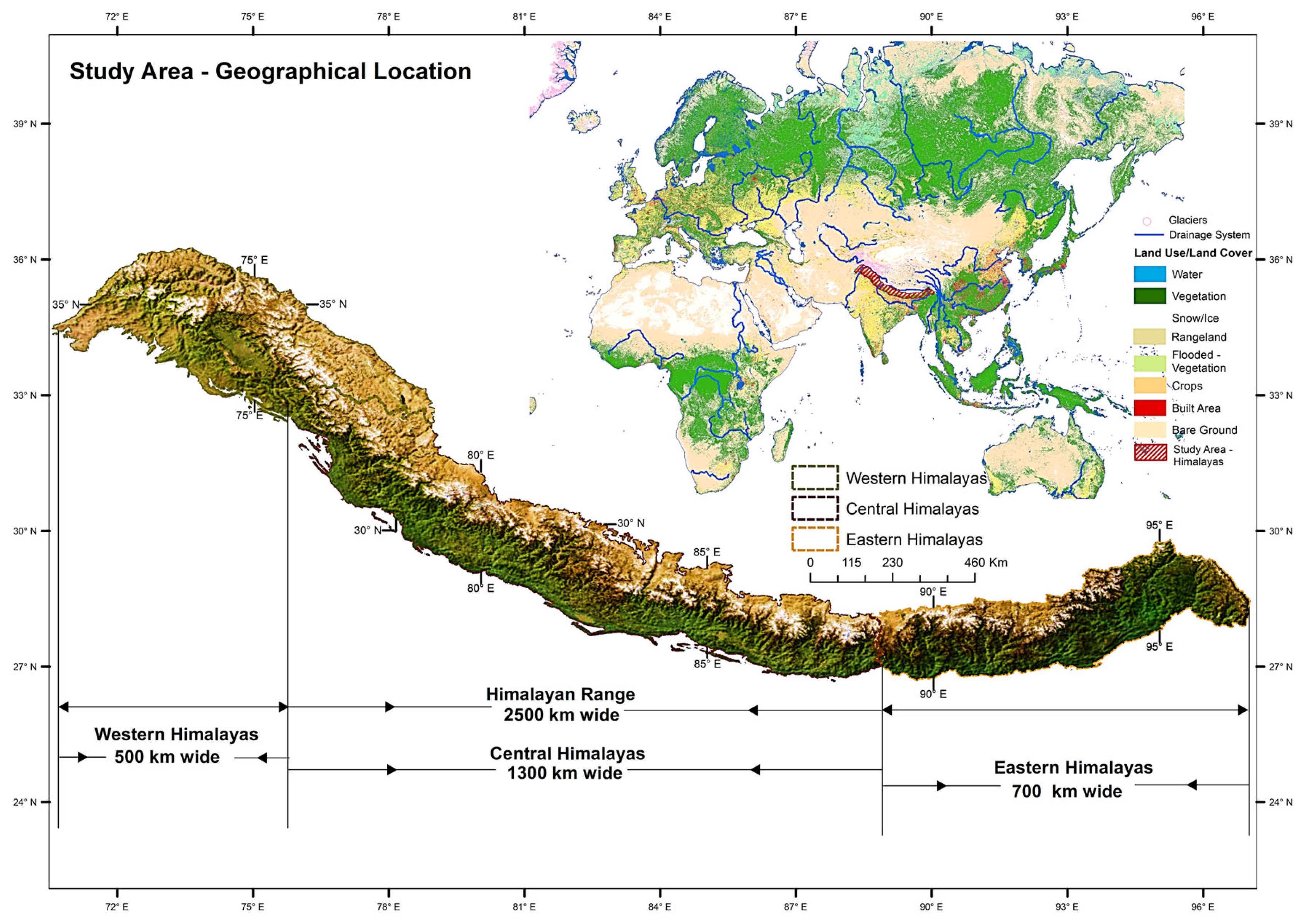
Figure 1. Geographical location of the study area is categorized into Western, Central, and Eastern Himalayas, extending across territories delineated by international borders.
Remotesensing 17 03175 g001
Figure 2. Schematic diagram of the research methodology.
Remotesensing 17 03175 g002
Figure 3. Normalized NDSI maps of the Himalayan snow-covered areas, showing inter-regional spatiotemporal variability from 2004 to 2024 with an interval of four years.
Remotesensing 17 03175 g003
Figure 4. Interannual variability in SCAs across the Himalayas and its sub-regions from 2004 to 2024, including the annual rate of change (ROC) representing the year-over-year percentage variation in SCA.
Remotesensing 17 03175 g004
Figure 5. Correlation between standardized SCA, Temperature (°C), and Precipitation (mm) from 2004 to 2024 across (a) Western Himalayas, (b) Central Himalayas, and (c) Eastern Himalayas.
Remotesensing 17 03175 g005
Figure 6. Map of pixel-level coefficient of variation (CV) for snow cover across the Western, Central, and Eastern Himalayas (2004–2024).
Remotesensing 17 03175 g006
Figure 7. Statistical evaluation of NDSI values across the Himalayas from 2004 to 2024, including the first, second, and third quartiles (Q1, Q2, and Q3). The 2-year moving average smooths short-term fluctuations and highlights underlying trends in snow cover dynamics over time.
Remotesensing 17 03175 g007
Figure 8. Trends in SCPs across the Western, Central, and Eastern Himalayas. (a) Total SCP count showing statistically significant (p ≤ 0.05) and non-significant (p > 0.05) trends based on the Mann-Kendall test; (b) Distribution of SCPs exhibiting upward (↑) and downward (↓) trends determined using Kendall’s τ correlation coefficient, highlighting the direction and strength of change.
Remotesensing 17 03175 g008
Figure 9. (ac) Elevation-specific distribution of SCPs with significant trend (at 5% significance level) for the WH, CH, and EH. The dotted lines represent the mean elevations across the respective trend; (df) Elevation-specific increasing and decreasing trend for the significantly changed SCPs; and (gi) Distribution of significantly changed SCPs with corresponding change-points year over the study period (2004–2024).
Remotesensing 17 03175 g009
Figure 10. Reconstructed SCAs at constant contour intervals with a hypsometric curve representing constant AAR (0.5 and 0.67) and AABR ratios (0.96 and 1.75) for (a) Western Himalayas (WH); (b) Central Himalayas (CH); and (c) Eastern Himalayas (EH).
Remotesensing 17 03175 g010
Figure 11. Elevation range of WH (a,b), CH (c,d), and EH (e,f) plotted against the cumulative SCA in percentage for constant AAR (0.4 to 0.8, with 0.05 interval) and AABR values (0.9 to 4.4, with 0.01 intervals).
Remotesensing 17 03175 g011
Table 1. Annual classification performance of MOD09A1-derived NDSI (2004–2024): Kappa coefficient, Overall Accuracy, Precision, Recall, F1 score, and Misclassification Rate.
YearTrue NegativeFalse
Positive
False
Negative
True
Positive
Overall
Accuracy
Precision (Snow)Recall (Snow)F1 ScoreKappa
Statistic
Misclassification Rate
(TN)(FP)(FN)(TP)(OA) (Ka)(MR)
200411,838,94877,92138,494682,4370.99080.89750.94660.92140.91650.0092
200511,641,374163,16122,526810,7390.98530.83250.97300.89720.88940.0147
200611,858,926124,24223,976630,6560.98830.83540.96340.89480.88870.0117
200711,710,598126,43929,097771,6660.98770.85920.96370.90840.90190.0123
200811,787,311111,82024,796713,8730.98920.86460.96640.91270.90690.0108
200911,835,63466,84425,012710,3100.99270.91400.96600.93930.93540.0073
201011,831,35946,17635,238725,0270.99360.94010.95370.94680.94340.0064
201111,766,435210,25616,287644,8220.98210.75410.97540.85060.84120.0179
201211,749,961227,13436,843623,8620.97910.73310.94420.82540.81450.0209
201311,654,108170,62133,045780,0260.98390.82050.95940.88450.87590.0161
201411,731,121185,07329,714691,8920.98300.78900.95880.86560.85670.0170
201511,646,289113,39925,108853,0040.98900.88270.97140.92490.91900.0110
201611,931,84474,46837,898593,5900.99110.88850.94000.91350.90890.0089
201711,849,531202,10613,932572,2310.98290.73900.97620.84120.83240.0171
201811,942,945104,63117,822572,4020.99030.84550.96980.90340.89830.0097
201911,573,962191,27021,768850,8000.98310.81650.97510.88870.87970.0169
202011,613,29964,16146,315914,0250.99130.93440.95180.94300.93830.0087
202111,934,85043,34246,142613,4660.99290.93400.93000.93200.92830.0071
202211,679,40579,43435,619843,3420.99090.91390.95950.93610.93120.0091
202311,918,07181,72531,951606,0530.99100.88120.94990.91430.90950.0090
202411,936,909209,14124,625467,1250.98150.69070.94990.79990.79040.0185
Mean11,817,98997,81826,273695,7200.99020.87670.96360.91810.91290.0098
Disclaimer/Publisher’s Note: The statements, opinions and data contained in all publications are solely those of the individual author(s) and contributor(s) and not of MDPI and/or the editor(s). MDPI and/or the editor(s) disclaim responsibility for any injury to people or property resulting from any ideas, methods, instructions or products referred to in the content.