Article

Long-Term Pan-Arctic Evaluation of a Sentinel-1 SAR Sea Ice Extent Product and Insights into Model Integration

1
Aerospace Information Research Institute, Chinese Academy of Sciences, Beijing 100094, China
2
University of Chinese Academy of Sciences, Beijing 100049, China
3
State Key Laboratory of Spatial Information System and Integrated Application, Beijing Institute of Satellite Information Engineering, Beijing 100095, China
*
Author to whom correspondence should be addressed.
Remote Sens. 2025, 17(18), 3166; https://doi.org/10.3390/rs17183166
Submission received: 26 July 2025 / Revised: 5 September 2025 / Accepted: 9 September 2025 / Published: 12 September 2025

Abstract

Highlights

What are the main findings?
  • A pan-Arctic sea ice extent product generated from over 85,000 Sentinel-1 images shows strong agreement with the AMSR2 sea ice concentration product and provides superior capability in depicting the marginal ice zone.
  • An Integrated Index is introduced to quantify sub-model contributions in the ensemble used for sea ice extent generation, revealing that three sub-models dominate the results.
What is the implication of the main finding?
  • The SAR-based sea ice extent product serves as reliable baseline data for both operational applications and scientific research.
  • The Integrated Index offers a methodological basis for optimizing integration strategies, with potential applications in future sea ice ensemble models.

Abstract

Reliable sea ice extent (SIE) information is essential for Arctic navigation, climate research, and resource exploration. Synthetic Aperture Radar (SAR), with its all-weather, high-resolution capabilities, is well suited for SIE extraction. This study evaluates a pan-Arctic SIE product automatically generated from over 85,000 Sentinel-1 SAR images acquired between 2020 and 2023 using an integrated stacking U-Net framework. To validate its performance, all the SIE products are converted to sea ice concentration (SIC) and compared against the 3.125 km resolution Advanced Microwave Scanning Radiometer-2 (AMSR2) SIC products. The S1-derived SIC shows strong agreement with AMSR2 SIC, yielding a Pearson correlation of 0.99 and annual mean absolute differences between 5.93% and 7.85%. Case analyses demonstrate that the S1 products effectively capture small-scale ice features, such as floes, which are often missed by AMSR2. Furthermore, we introduce an Integrated Index to quantify the relative contribution of each sub-model within the integrated stacking U-Net framework. The analysis indicates that three sub-models provide the primary contribution to the ensemble, offering insights into improving integration efficiency and guiding the design of more scientifically grounded ensemble strategies.

1. Introduction

Sea ice extent (SIE) is a critical indicator for monitoring Arctic sea ice conditions, carrying significant implications for navigation safety [1], resource exploration [2], and climate change research [3]. Remote sensing techniques, with extensive spatial coverage and frequent revisit capabilities, have become indispensable for large-scale, continuous monitoring of Arctic SIE [4,5,6].
Spaceborne microwave radiometers have been fundamental to sea ice concentration (SIC) and SIE mapping, given their all-weather, day-and-night observation capabilities and stable pan-Arctic daily coverage [7,8,9]. These sensors exploit the microwave emissivity contrasts between sea ice and open water to derive SIC from brightness temperature measurements. SIC and SIE can be interconverted by applying concentration thresholds and spatial aggregation, enabling consistent and widespread applications [10,11]. Continuous SIC monitoring has been achievable since the late 1970s, with notable missions such as the Nimbus-7 Scanning Multichannel Microwave Radiometer (SMMR), Special Sensor Microwave Imager (SSM/I), Defense Meteorological Satellite Program (DMSP) and Advanced Microwave Scanning Radiometer-2 (AMSR2). AMSR2, specifically, offers relatively high spatial resolution and is widely employed for generating operational SIC products [7,12,13]. For example, the University of Bremen utilizes the ARTIST sea ice (ASI) algorithm on AMSR2 data to produce SIC products at spatial resolutions of 6.25 km and 3.125 km [14]. However, the kilometer-scale resolution remains insufficient for capturing small-scale sea ice features, such as ice floes and leads [15].
Synthetic Aperture Radar (SAR), characterized by high spatial resolution and all-weather imaging capabilities, provides an essential complementary approach. In particular, the Sentinel-1 (S1) constellation, featuring dual-polarization Extra Wide (EW) mode imaging with approximately 40 m resolution and 400 km swath width, delivers over 2500 Arctic images monthly, making it highly suitable for detailed SIE mapping. Nevertheless, reliable, large-scale, and long-term SIE automated extraction from S1 data presents challenges, including radar backscatter ambiguities across ice types, variability in open water roughness under varying wind conditions, sensor noise, and sensitivity to incidence angles [16].
Recent advancements in deep learning methods, renowned for their exceptional feature extraction capabilities, have facilitated new approaches for automatic SIE extraction. In our prior research, we developed an integrated stacking framework composed of multiple scenario-specific U-Net models, a widely utilized deep learning architecture for image segmentation [17,18,19,20,21], trained on S1 EW mode data [22]. This framework enables the automated generation of standardized pan-Arctic SIE products at a spatial resolution of 400 m in Network Common Data Form version 3 (NetCDF-3) format. Cross-validation with Arctic data from 2019 demonstrates promising accuracy, yielding an annual mean absolute difference of 5.55% relative to the AMSR2 6.25 km SIC product and a 93.98% agreement rate with the NOAA Interactive Multisensor Snow and Ice Mapping System (IMS) SIE product [22]. The S1 SIE products were publicly available through the Science Data Bank until 2021, with cumulative downloads exceeding 66,500, and have since been integrated into the National Earth Observation Data Center (NODA), underscoring their growing recognition within the research community. In addition to providing direct, high-resolution SIE information, this product also offers substantial value for constructing more accurate region-specific models. By fine-tuning on this product, researchers can efficiently obtain accurate training labels, thereby facilitating the development of regional models without extensive manual annotation.
Following the launch of Sentinel-1C, the Sentinel-1 constellation has resumed sufficient data coverage necessary for Arctic SIE product generation. Accordingly, we plan to further process and release this product to the public. This study presents a comprehensive evaluation of the S1 SIE product, generated from over 85,000 S1 EW-mode images collected between 2020 and 2023, to support the next phase of product releases. We used the AMSR2 3.125 km resolution SIC product from the University of Bremen for cross-validation, as it provides consistent daily pan-Arctic coverage and a long-term time series since 2002, ensuring stable applicability. Case studies illustrate the complementary strengths of the two datasets: the S1 product offers enhanced detail in marginal ice zones, while AMSR2 provides stable performance in high-concentration sea ice regions. Further evaluation with data from the newly launched Sentinel-1C satellite confirms that the workflow developed for SIE product generation remains robust and generalizable to new sensor inputs. An Integrated Index is introduced to quantify the contribution of each sub-model within the integrated U-Net framework used for SIE product generation, providing a foundation for streamlining the model and designing more scientifically grounded integration strategies. In addition, we further analyze the product’s applicability, the possible causes of the increased differences, and potential approaches for future improvements. It should be noted that AMSR2 SIC is not regarded as the absolute ground truth in this study, but rather as an authoritative and stable reference dataset. It is employed to assess, on a broad spatial scale, whether the deep learning-derived S1 SIE product exhibits pronounced generalization issues under varying sea-ice conditions, as well as to evaluate its potential to complement the AMSR2 product.

2. Data

2.1. Sentinel-1 Data

85707 S1 EW mode dual-polarization (HH and HV) images acquired across the Arctic between 2020 and 2023 are employed to generate SIE products. The data are provided in the ground range detected medium resolution (GRDM) format, featuring a spatial resolution of 40 m × 40 m. Each image covers approximately 400 × 400 km, with incidence angles ranging from 18.9° to 47.0°, making these data well suited for Arctic sea ice monitoring by balancing spatial resolution and observation coverage.

2.2. Sentinel-1 SIE Product

Based on preprocessed S1 EW dual-polarization data, we generate a total of 85,707 SIE products using the integrated stacking U-Net architecture proposed by Wang and Li [22]. Each product contains information on geographic location, sea ice, and land, provided at a spatial resolution of 400 m. As illustrated in Figure 1, we present a visualization of a preprocessed S1 image alongside the corresponding SIE product, where dark gray denotes land, cyan represents open water, and yellow indicates sea ice. The detailed storage format of the product is provided in Table 1. Each is stored in NetCDF-3 format and comprises four variables: Longitude, Latitude, SeaIce, and Mask. For the SeaIce variable, a value of 0 corresponds to open water, whereas a value of 1 denotes the presence of sea ice. In addition, the Mask variable uses 0 to indicate oceanic or ice-covered regions (non-land), while 1 signifies land areas. Figure 2 displays the monthly distribution and proportion of the products from 2020 to 2023, showing a relatively lower number during May, June, and July, which is constrained by the reduced availability of S1 EW-mode acquisitions in these months, possibly due to mission planning priorities of the S1 satellites.

2.3. AMSR2 SIC Product

The daily AMSR2 SIC product with a spatial resolution of 3.125 km, released by the University of Bremen [23], is employed for comparison with the S1 SIE product. The AMSR2 SIC data are primarily retrieved using the ASI algorithm, which combines an empirical model for SIC retrieval with a statistical model to account for atmospheric influences [14]. The ASI algorithm predominantly relies on the polarization difference between vertically and horizontally polarized brightness temperatures at 89 GHz.

3. Methods

This section primarily describes the main workflow for generating SIE products from S1 imagery, as well as the spatiotemporal matching method between the S1 SIE products and the AMSR2 SIC products. More detailed methodologies can be found in the studies by Wang and Li et al. [22].

3.1. Workflow of SIE Product Generation

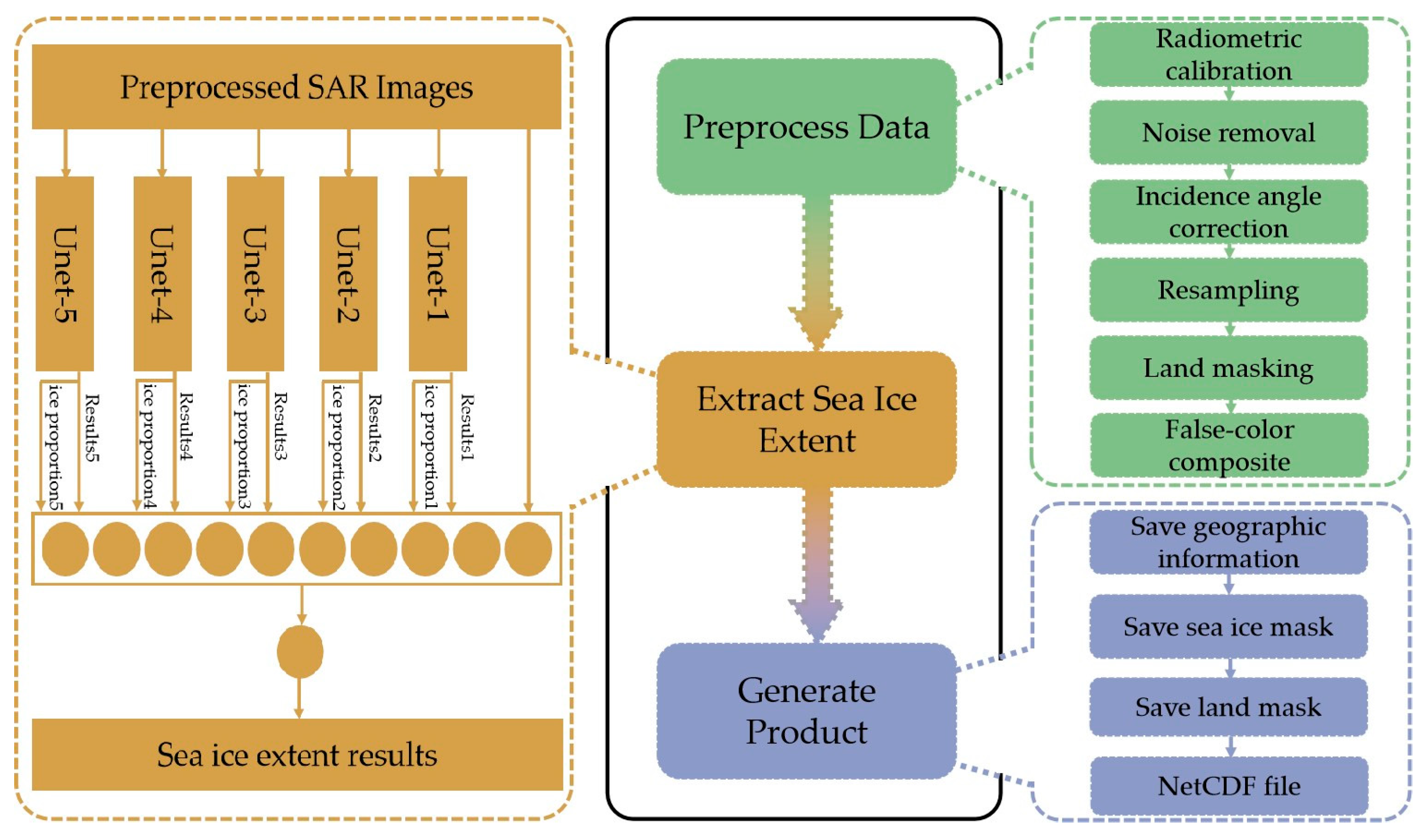
Figure 3 illustrates the workflow for generating SIE products from S1 images. The dual-polarization S1 EW images first undergo preprocessing steps, including radiometric calibration, noise removal, incidence angle correction, land masking, and the generation of false-color composites. Both HH and HV polarization images are radiometrically calibrated. To address scalloping effects and thermal noise, particularly prominent in HV polarization, the denoising method proposed by Sun and Li [24] is applied. This method segments the images into azimuthal blocks and refines the standard noise vectors provided with S1 data using improved scaling and balancing factors, effectively removing residual noise at sub-swath boundaries. The HH polarization data are then corrected for incidence angle effects using the linear regression approach introduced by Murashkin et al. [25]. The data are subsequently downsampled by a factor of 10 using a 10 × 10 mean window, resulting in a spatial resolution of 400 m. Land areas are masked using the Global Self-consistent Hierarchical High-resolution Geography Database (GSHHG). Finally, the polarization difference and ratio between HH and HV channels are computed and combined with the HV polarization images to generate false-color composite images, which are linearly stretched to a pixel value range of 0–255.
Subsequently, the preprocessed images are input into an integrated stacking U-Net model. Five scenario-specific sub-U-Net models are first applied to extract sea ice, each producing a SIE map and estimating the proportion of sea ice pixels. Notably, in the design of the sub-models, Models 2 and 3 are more effective at identifying large areas of sea ice, particularly newly formed ice. Models 1 and 4 yield fewer misclassifications over high-wind sea surfaces. Models 3 and 5 capture finer details in regions where sea ice is mixed with open water [22]. These outputs, along with the corresponding false-color composite images, are collectively passed to a hidden layer comprising ten neurons. A final output neuron then aggregates the hidden layer results to generate the final SIE. The geographic coordinates for each pixel, together with the derived sea ice and land masks, are stored in NetCDF-3 format to produce the SIE products.

3.2. Matching and SIC Calculation Method

We compare the S1 SIE products with the AMSR2 SIC products. Temporal alignment is achieved by matching the acquisition dates indicated in the image IDs of both datasets. For spatial alignment, the S1 products, originally at a resolution of 400 m, are resampled to a regular 3.125 km grid to match the spatial resolution of the AMSR2 data. The four corner coordinates of each S1 image are extracted, and their corresponding locations within the AMSR2 grid are identified using a nearest-neighbor search. Based on this mapping, the AMSR2 SIC data are spatially subset to match the geographic coverage of each S1 image.
For pixel-wise comparison, a cell-based matching approach is employed. Specifically, each AMSR2 grid cell is represented by four corner coordinates, which are derived through spatial interpolation of the original grid cell coordinates. This interpolation yields a fine-resolution geographic mesh, enabling delineation of each AMSR2 grid cell’s geographic boundaries. For each cell, the set of S1 pixels falling within its spatial extent is identified based on their geolocated coordinates.
Subsequently, the proportions of sea ice and open water pixels are calculated for each AMSR2 grid cell using the corresponding S1 pixels, while land pixels, determined using a land mask, are excluded from the analysis. If the proportion of land pixels within a cell is less than 50%, the S I C S A R is calculated as the percentage of sea ice pixels relative to the total number of sea ice and open water pixels, as defined in Equation (1). Otherwise, the cell is classified as land and excluded from further comparison.
S I C S A R = n i c e n i c e + n w a t e r
Here, n i c e represents the number of sea ice pixels, while n w a t e r represents the number of open water pixels.

3.3. Evaluation Metric

The absolute difference is used to evaluate the bias between the S1 SIC and the AMSR2 SIC, as shown in Equation (2).
A b s o l u t e   d i f f e r e n c e = | S I C S A R S I C A M S R 2 |
where S I C A M S R 2 represents the SIC of the AMSR2 product.

3.4. Integrated INDEX

As shown in Figure 3, the five sub-models used in the integrated U-Net framework were selected based on expert knowledge, without a strict quantitative assessment of their contributions to the ensemble. Therefore, this study proposes an Integrated Index to quantitatively evaluate the importance of each sub-model within the ensemble. This index comprises two components: the difference between each individual model and the integrated result, and the pairwise differences among the individual models themselves. The rationale is twofold. First, a smaller difference between an individual model and the integrated output indicates that the model’s information has been more substantially adopted in the integration, reflecting greater importance. Second, model diversity is a critical factor in integration-based learning [26,27]. The complementary differences among models also play an important role in enhancing the effectiveness of the ensemble.
To quantify inter-model differences, we employ the Dice Similarity Coefficient (DSC), a metric widely used in image segmentation tasks [26,27,28]. The calculation of this metric is as follows:
D S C ( A , B ) = 2 | A B | A + | B |
Here, A and B are the sets of sea ice pixels from the two extraction results being compared, respectively. | A B | denotes the number of overlapping pixels, and A , | B | represent the total number of sea ice pixels in each result. The DSC from 0 (no overlap) to 1 (perfect agreement), and it is symmetric: swapping A and B yields the same result. Based on this metric, we define the Integrated Index for each model as follows:
I n t e g r a t e d   I n d e x =   α · ( 1 D S C M i , M i n t ) + β · 1 N 1 Σ i j D S C M i , M j
Here, M i denotes the extraction result of the i t h model, M i n t is the integrated result, and N is the total number of models. The parameters α and β are adjustable weights, both of which are set to 1 in this study. A smaller value of the Integrated Index indicates a greater contribution. The proposed index provides a scientifically grounded basis for selecting more appropriate ensemble strategies, thereby ensuring that model integration remains both efficient and robust under varying sea ice conditions. It should be noted that the purpose of this index is not to further improve the accuracy of the ensemble model.

4. Results

4.1. Statistical Analysis

For quantitative evaluation, we calculate the absolute pixel-wise SIC differences between the S1 and AMSR2 products for each image and average these values across all pixels within each image. Daily mean absolute differences are then obtained by averaging the image-level values for all images acquired on the same day. The annual mean absolute differences, calculated as the average of daily means, are 6.72% in 2020, 5.93% in 2021, 7.54% in 2022, and 7.85% in 2023. This approach ensures that each day is weighted equally in the annual statistics, thereby minimizing potential bias arising from uneven observation frequency or coverage across different days. Since sea ice conditions can vary substantially over time due to dynamic environmental influences, calculating daily mean absolute differences before annual aggregation provides a more representative and temporally balanced assessment of product performance throughout the year.
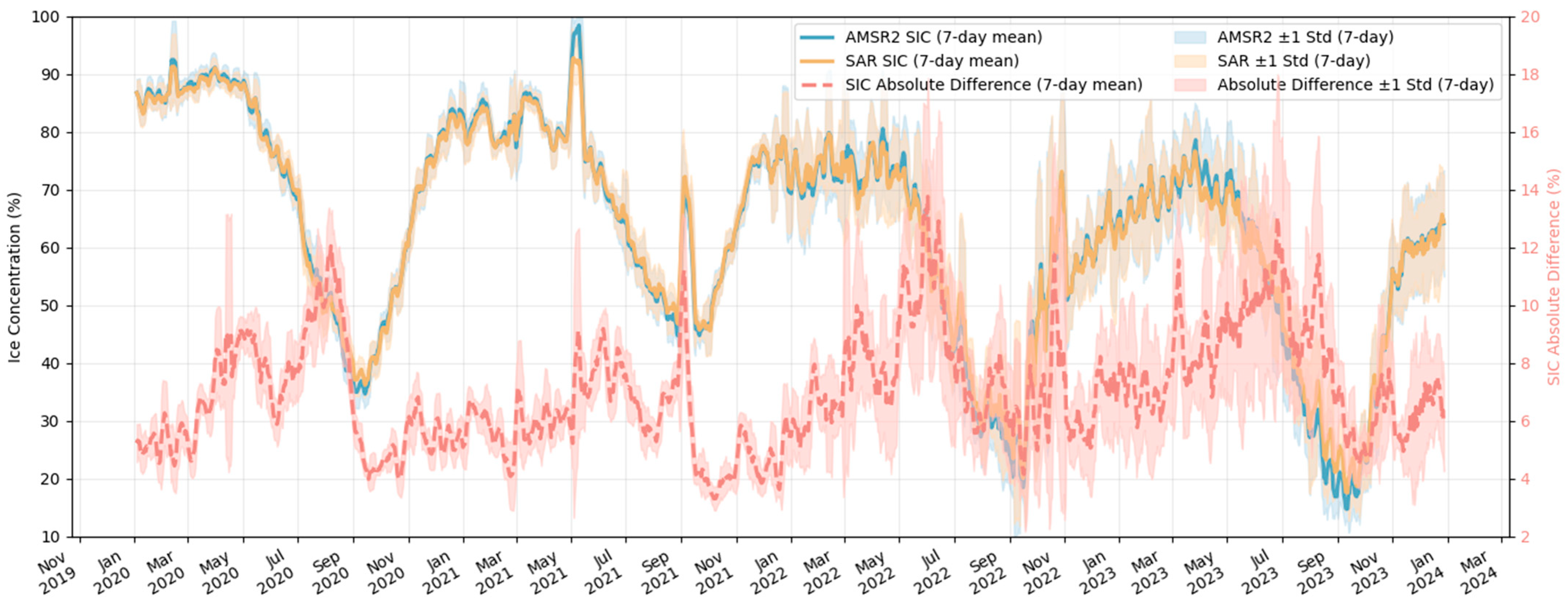
The daily variations of SIC and the differences are plotted, as shown in Figure 4, after applying a seven-day moving average for smoothing. The shaded bands represent the standard deviation within each seven-day window. The yellow line represents the SIC derived from the S1 SIE products, while the blue line indicates the AMSR2 SIC. The two curves exhibit strong consistency, with a Pearson’s coefficient of 0.99. The red line shows the daily variation of the absolute difference between the two products, which remains below 10% for most of the period.
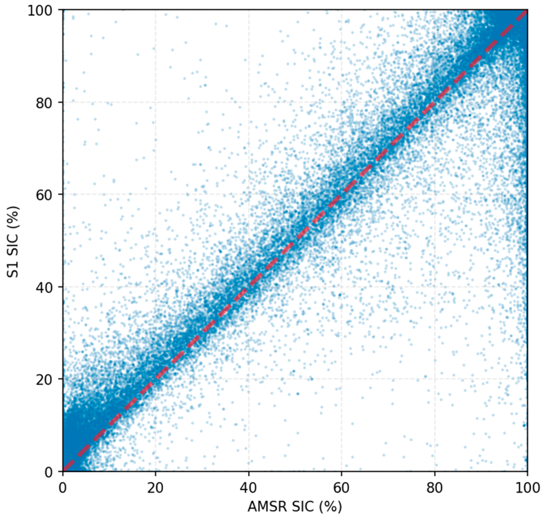
In addition, to better characterize the relationship between the AMSR2-derived SIC and the S1-derived SIC, we visualized their scatterplot as shown in Figure 5. The data points are largely distributed along the one-to-one line, indicating strong overall consistency between the two products. Notably, in areas with low SIC, the S1-derived values tend to exceed those from AMSR2, suggesting that our S1 product may provide improved representation of sea ice conditions in low-concentration regions.
To identify the overall timing of high-difference occurrences (>10%), we first examine the trend of the monthly mean absolute differences, as shown in Figure 6. The multi-year mean difference curve indicates elevated differences during the melt season from May to August. The possible reason for the reduced differences observed in September is that this period corresponds to the annual peak of sea ice melt, during which extensive open-water conditions prevail [11]. Under the condition, both S1 and AMSR2 SIC estimates can be obtained with relatively high accuracy.
Furthermore, Figure 7 illustrates the spatial distribution of product differences from May to August during 2020–2023, with each point representing the geographic center of a product. Red points denote differences exceeding 40%, orange indicates 30–40%, yellow represents 20–30%, green corresponds to 10–20%, and blue indicates differences below 10%.
A clear concentration of high-difference cases is observed in near-coastal areas, particularly around the Canadian Arctic Archipelago and the coast of Greenland. This phenomenon can be easily attributed to several factors. AMSR2 products are notably affected by land spill-over contamination, resulting in elevated errors, an issue that has been extensively documented in previous studies [15] and the ASI Version 5 Sea Ice Concentration User Guide [23]. For the S1 products, misalignment between the land mask and the actual coastline in the imagery can lead to incomplete masking of land areas. These unmasked land pixels, characterized by high radar backscatter, are frequently misclassified as sea ice by the algorithm. Additionally, the discrepancy in coastline delineation resulting from the differing spatial resolutions of the two products can significantly contribute to the differences between them. The combined impact of these sources of error contributes to substantial discrepancies along coastal zones. Therefore, in such cases, these two products should be used with caution.
In offshore regions, notably the Beaufort–Chukchi and East Siberian Seas, elevated differences are frequently observed during July and August of 2020–2023. In this context, the sources of difference should be discussed in greater detail, as they reflect the complementary characteristics of the two products under stable application scenarios. Accordingly, representative high-difference cases from these regions are selected for further analysis.

4.2. Case Analysis

We select a total of four cases with high differences (>10%) from the East Siberian Sea and the Chukchi–Beaufort Sea regions for further analysis. As shown in Figure 8b, the image captured on 28 August 2020, over the eastern Chukchi Sea serves as the primary image for analysis. The S1 SIE product shown in Figure 8d calculated an image-averaged SIC of 14%, with a difference of 12% compared to the AMSR2 product. As illustrated in Figure 8f, the AMSR2 product substantially underestimates sea ice in this region, whereas the S1 SIE and SIC effectively capture the presence, as shown in Figure 8d,e. Given that sea ice can change rapidly in regions with low SIC, it is important to exclude potential differences arising from the temporal gap between data acquisitions. Therefore, we examine images acquired on the preceding and following days, as shown within the red boxes in Figure 8a,c, respectively. The presence of ice floes in this area on both days suggests that sea ice was likely present within the temporal window surrounding the target observation date.
Figure 9b shows the S1A image captured on August 7 over the Chukchi Sea, with the S1 SIE product estimating a image-averaged SIC of 94% and difference of 22% compared to the AMSR2 product. Similar to the case presented in Figure 8, the AMSR2 product exhibits substantial omissions in capturing SIE in this region, as shown in Figure 9f, while the S1 SIE and SIC effectively captures the presence of sea ice, as illustrated in Figure 9d,e. However, the S1 product tends to overestimate SIC in this case, likely due to the downsampling operations in the deep learning framework. These operations may obscure spatial detail, causing densely packed ice floes to resemble continuous sea ice and leading to their misclassification as such [29]. Figure 10 presents the transition zone between the Chukchi Sea and the East Siberian Sea, where a similar situation is observed, with a difference of 47%.
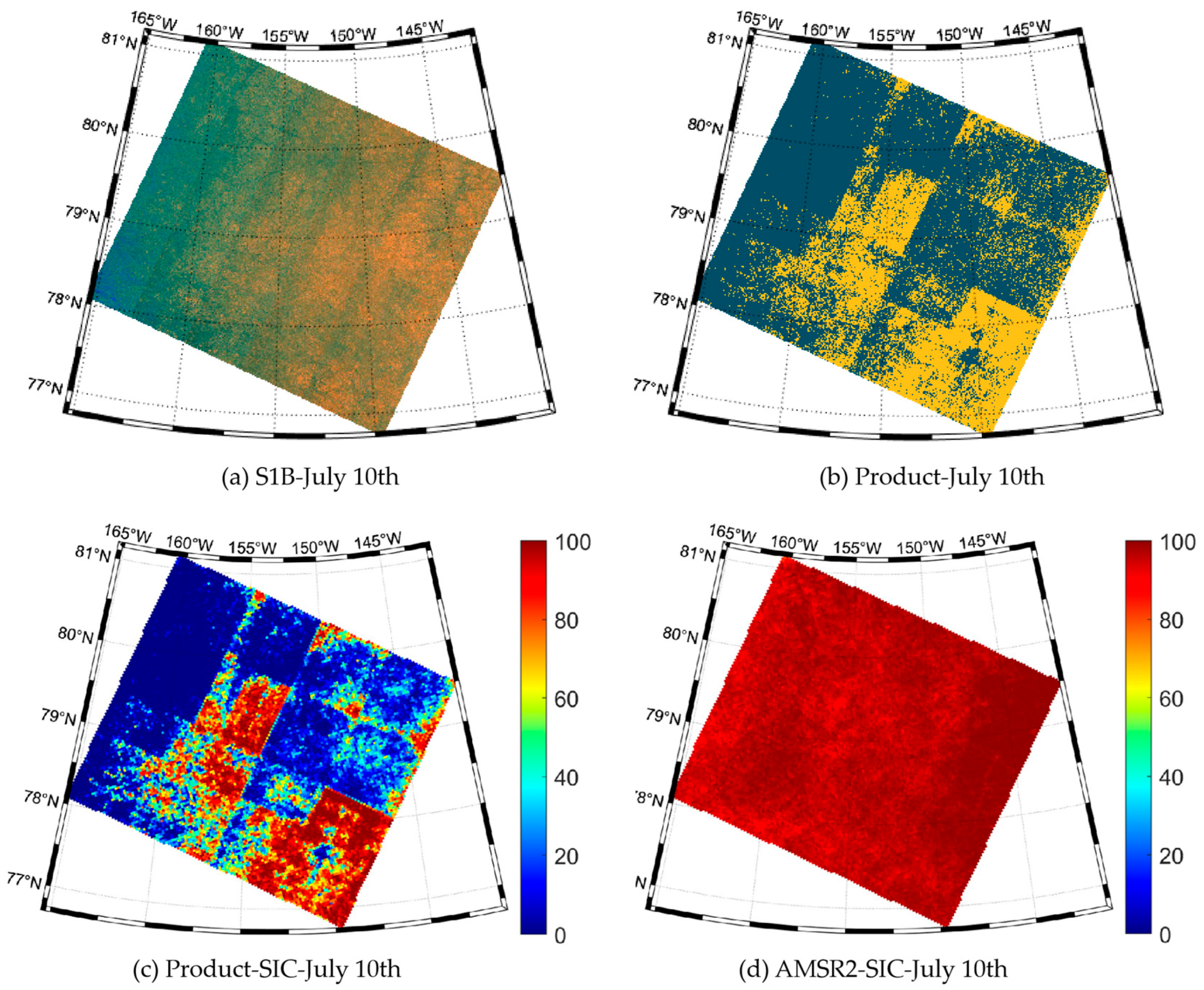
Figure 11 presents images near the central Arctic region, located north of the Beaufort Sea, with image-averaged mean absolute differences of 59%. The region exhibits high SIC, where the S1 SIE product encounters occasional generalization issues, while the AMSR2 product provides a more stable representation of SIC. In conclusion, in marginal ice zones with the presence of ice floes, S1 products can effectively compensate for the underestimation observed in AMSR2 products. In contrast, in the high-latitude central Arctic region, AMSR2 may provide more stable sea ice information. The combined use of both products enables a more detailed and accurate characterization of Arctic sea ice.

4.3. Accuracy Validation of Sentinel-1C Products

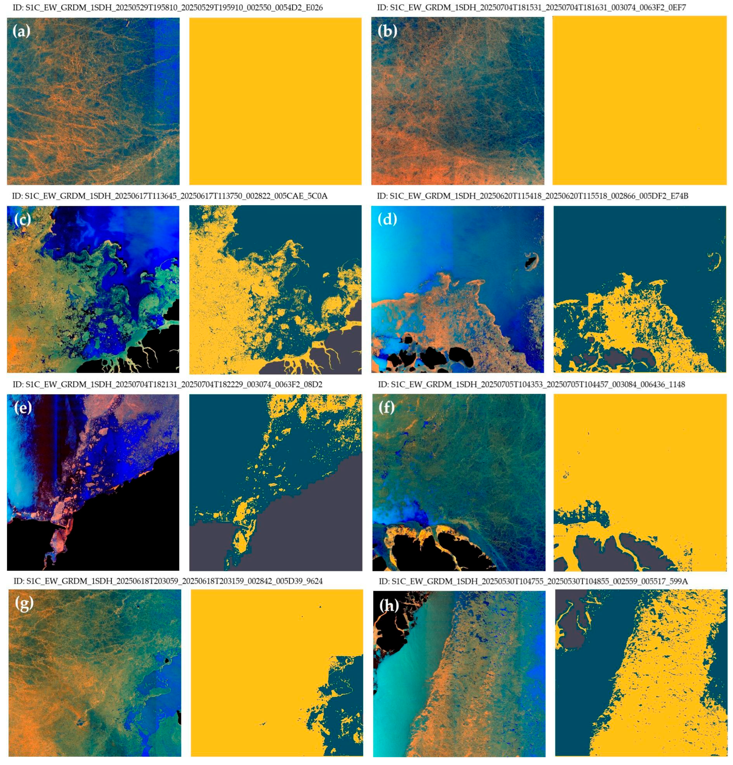
We note that Sentinel-1C has been deployed as a replacement for Sentinel-1B after its loss of communication and has since provided stable observations over the Arctic. Although the two satellites share identical technical specifications, even minor differences in image quality may lead to generalization issues for deep learning-based SIE mapping methods [28], since the existing models have been trained exclusively on Sentinel-1A/B data. To assess the generalization capability of our approach, we process 8 Sentinel-1C images acquired during the 2025 melt seasons (May 2025 to July 2025) using the same SIE product generation workflow described in Section 3.1. As shown in Figure 12a,b, the proposed method remains stable in regions with high SIC. Moreover, as illustrated in Figure 12c–h, it continues to effectively capture small-scale sea ice features in the marginal ice zone, maintaining its advantages.

4.4. Sub-Model Contribution Analysis

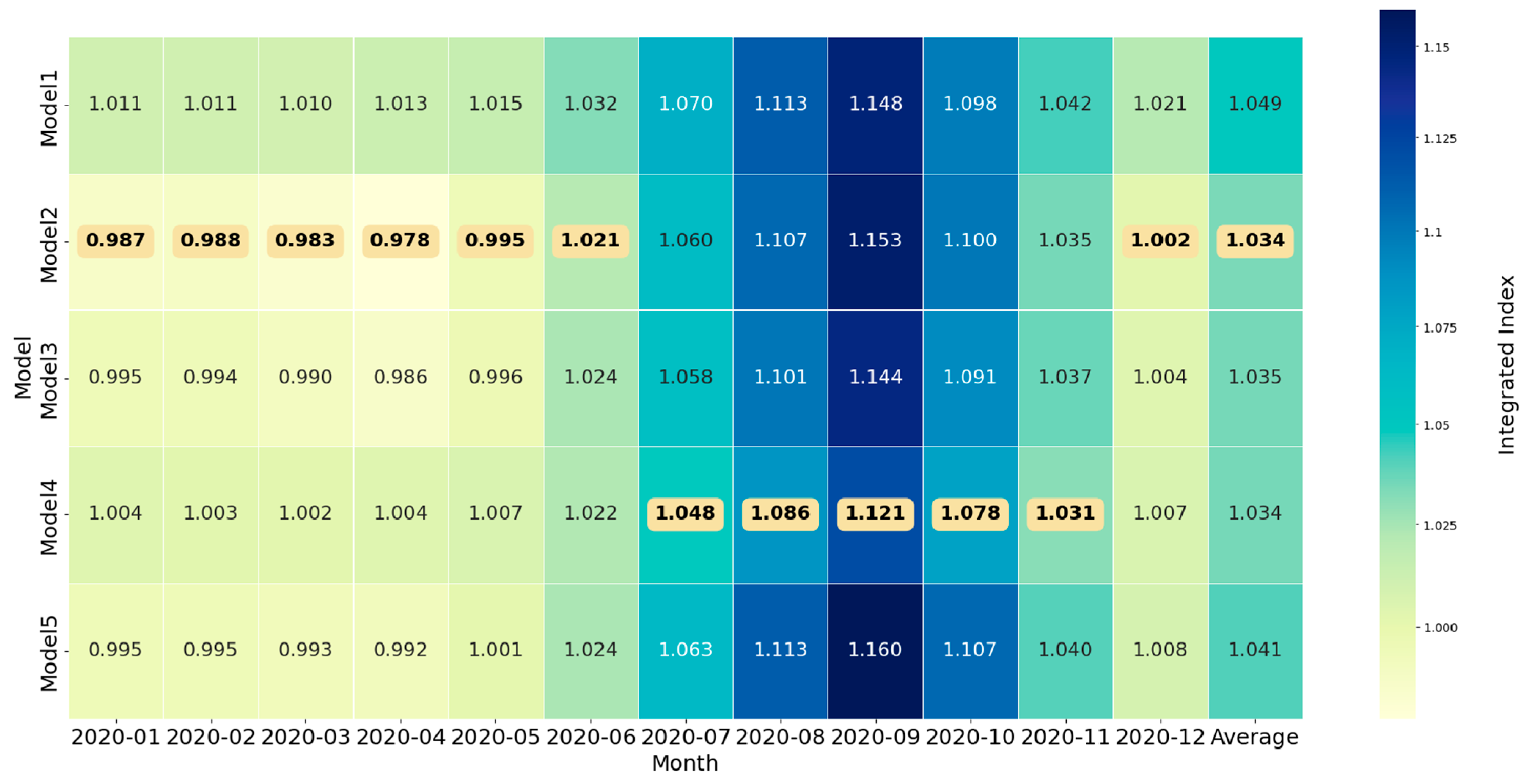
As shown in Figure 13, the monthly Integrated Index values for the year 2020, along with the annual average, are presented. Model 2 (January–June and December) and Model 4 (July–November) together account for all the months with the lowest index values, indicating the highest contribution across the year. In contrast, Model 1 (January–July, November, and December) and Model 5 (August–October) are responsible for the months with the highest index values, reflecting the lowest contribution levels. Model 3 consistently ranks as the second most contributing model in ten out of twelve months (January–May, July–October, and December). The annual average contribution ranks from highest to lowest as follows: Model 2 (1.034), Model 4 (1.034), Model 3 (1.035), Model 5 (1.041), and Model 1 (1.049). Therefore, in scenarios where computational efficiency or real-time processing is prioritized, Model 1 and Model 5 should be considered for removal, while Models 2, 3, and 4 are recommended to be retained to maintain integration effectiveness. At the same time, we observe that the Integrated Index remains relatively stable from January to June. Starting in July, however, the index exhibits a general upward trend, peaking in September, and gradually decreases thereafter. This pattern may be attributed to changes in the integration mechanism of the ensemble model. To further investigate this, we visualize the two components of the Integrated Index for each model and month, namely, the difference between each model and the ensemble output (hereafter referred to as 1–DSC), and the similarity among sub-models (hereafter referred to as DSC), as shown in Figure 14.
Figure 14 presents the monthly values of 1–DSC between each sub-model and the ensemble result, alongside the mean pairwise DSC among sub-models. Each model is thus represented by two adjacent columns for each month. It can be observed that starting in July, the values of 1–DSC increase significantly, peaking around September, and then begin to decline, returning to levels similar to those in January–June by November and stabilizing by December. This pattern indicates a substantial divergence between the outputs of individual models and the ensemble during July to November, suggesting that individual model predictions are less reliable in this period.
Meanwhile, the DSC among sub-models decreases markedly during the same months, reflecting greater diversity and disagreement among the sub-models. This increase in model diversity implies stronger complementarity, which may explain why the ensemble model maintains stable accuracy from July to November despite the degraded reliability of individual models. This phenomenon is understandable given the intensified sea ice melting observed during July to September, which complicates SIE extraction and challenges the robustness of individual models across the pan-Arctic. By October, as sea ice begins to refreeze and conditions gradually return to those observed earlier in the year, model consistency improves.
Considering the above, in accuracy-oriented applications, it is recommended to retain all sub-models during the July–November period to ensure sufficient model diversity. Moreover, adopting seasonally adaptive integration strategies may represent a promising direction for future optimization of the ensemble framework. For example, a reduced ensemble consisting of only Models 2 and 3 could be used from December of the previous year to June of the following year, while a full five-model ensemble can be employed from July to November.

5. Discussion

5.1. Applicability and Limitations of 400 m SAR-Derived SIE Products

Our results demonstrate that the 400 m resolution SAR-derived SIE product provides clear advantages over passive microwave radiometer products (e.g., AMSR2, 3.125 km), particularly in the marginal ice zone (MIZ), where small-scale floes and complex ice structures are more prevalent. Since most Arctic vessels tend to navigate along or across the MIZ, the ability to resolve these smaller floes is highly valuable for navigation [8]. However, the 400 m information is more suitable as a warning or situational awareness tool, enabling vessels to identify the presence and approximate distribution of floe bands. When ships attempt to actually cross the MIZ, shipborne radar, visual observation, and local ice reconnaissance remain indispensable for avoiding hazardous ice floes.
Beyond direct navigation support, the greatest potential of the S1-derived SIE product lies in its role as a complementary dataset to passive microwave observations. Passive microwave products provide consistent daily pan-Arctic coverage, while S1 observations typically require several days to complete a full Arctic mosaic. Accordingly, the S1-derived product should be regarded as an important supplement that enhances passive microwave products through data fusion, assimilation, and improved representation of marginal ice features, as has been demonstrated in a previous study [30].
In addition, the S1 SIE product can serve as a form of pseudo-labeling for subsequent research, supporting the development of more refined training datasets. By adjusting and refining these products, the workload of manual annotation can be reduced, thereby facilitating the training of higher-precision automated SIE extraction models, as demonstrated in the study of Wang et al. [31].

5.2. Impact of the Sentinel-1 Constellation Degradation on Temporal Variability

As shown in Figure 4, both the SIC time series and the difference curves exhibit a marked increase in standard deviation in 2022 and 2023, together with larger overall differences. While a certain degree of algorithmic instability cannot be fully excluded, these patterns appear plausibly linked to changes in the observing system and sampling characteristics. During the dual-satellite phase, the higher revisit frequency of Sentinel-1 enabled more continuous tracking of short-term sea ice evolution, such as floe formation, melt, or redistribution, thereby helping to maintain relatively smooth temporal statistics. In contrast, the single-satellite configuration in 2022–2023 resulted in substantially longer revisit intervals. Rapid ice changes are therefore sampled less frequently and often manifest in the time series as abrupt transitions, inflating the apparent variability. In addition, S1A acquisitions during this period, according to the European Space Agency’s official report Status of Copernicus Sentinel-1, Sentinel-1 Next Generation and ESA’s Earth Explorer 10 Harmony, are more concentrated at lower latitudes, where the MIZ is both more extensive and dynamic. The inherently higher variability and retrieval challenges in the MIZ likely further contributed to the increased standard deviations and differences. Nevertheless, this interpretation remains tentative, and further confirmation through quantitative analyses of acquisition frequency, spatial coverage, and contemporaneous sea ice conditions would be valuable.

5.3. Future Improvements

This section outlines potential improvements targeting the major limitation observed in the existing framework. To address the mismatch between the external coastline data and the shoreline boundaries observed in S1 imagery, as noted in Section 4.2, machine learning approaches can be employed to extract more accurate land–water boundaries. Specifically, the external coastline data can be used as a reference to manually delineate more precise shorelines on S1 imagery through visual interpretation, thereby constructing a labeled training dataset. A land segmentation classifier can then be trained using machine learning techniques. Several studies have already explored approaches for this purpose [32,33].
In addition, as shown in Figure 15, which corresponds to the issues observed in Figure 11, an occasional accuracy issue is detected in the current product, typically occurring in regions with high SIC. Although visual inspection of the 2020 dataset indicates that this issue is relatively infrequent, it may cause significant problems in certain applications. For instance, in assessments of SIE variability, anomalously low concentration values may appear in high-latitude areas. Also, non-expert users conducting route planning may misinterpret these regions as navigable without noticing the error.
It is evident that the issues in Figure 15a primarily originate from Model 2 and Model 3, while those in Figure 15b are mainly attributed to Model 3. This is due to the fact that sea ice extraction in the sub-models is performed using 256 × 256 image tiles, which are later stitched together to produce the full-scene result. When the accuracy of tile-based predictions is insufficient, the resulting errors in the full-scene output often manifest as rectangular false extractions corresponding to the tile shape. A potential solution is to fine-tune the current models using entire images and their corresponding labels. Given that the imagery is downsampled by a factor of 10 to a resolution of 400 m, resulting in image sizes of approximately 1000 × 1000 pixels, full-scene fine-tuning is computationally feasible. However, fine-tuning all sub-models may alter their functional roles within the ensemble, and it is therefore necessary to re-evaluate whether the ensemble composed of the five fine-tuned sub-models can still maintain robust performance across the pan-Arctic region.
Therefore, we tend to focus on adjusting the integration strategy rather than modifying the sub-models. In Figure 15a, Mode l1, Mode l4, and Mode l5 produce relatively accurate results, but the current integration strategy fails to adequately incorporate their outputs. A similar situation is observed in Figure 15b. We attribute this to the lack of targeted weighting across sub-model outputs within the integration framework. To address this, the attention mechanism [34,35,36] could be introduced to model sub-model contributions from both spatial and channel perspectives, enabling adaptive weighting that emphasizes more reliable extractions during the integration process.

6. Conclusions

This study evaluated the accuracy and generalization capability of a pan-Arctic SIE product generated using an integrated stacking U-Net model, based on 85,707 S1 EW mode SAR images from 2020 to 2023. Comparison against the widely used 3.125 km AMSR2 SIC product reveals a high Pearson correlation of 0.99, with annual mean absolute differences ranging from 5.93% to 7.85%. These results demonstrate the reliability and consistency of the S1 SIE product over long periods and across the entire Arctic region.
The analysis of monthly mean absolute difference trends and spatial distribution maps indicates that the highest discrepancies occur between May and August, with pronounced differences concentrated in nearshore regions, particularly around the Canadian Archipelago and Greenland. An analysis of the product generation workflows suggests that these discrepancies are primarily caused by interference from land-contaminated mixed pixels in the AMSR2 product, as well as limited accuracy in aligning the S1 imagery with the land mask, which can result in the omission of land pixels. Additionally, differences in spatial resolution between the two datasets contribute to subtle coastline mismatches, further amplifying the differences in these regions. Therefore, both products should be used with caution in these regions. In offshore regions, the differences are primarily concentrated in July and August within the Chukchi–Beaufort and East Siberian Seas. Case studies of high-difference images (>10%) further demonstrated that the S1 products are capable of capturing small-scale features, such as ice floes in marginal ice zones, which are often underrepresented in AMSR2 products due to resolution limitations. In contrast, the S1 product may exhibit occasional generalization issues under conditions of high SIC, whereas the AMSR2 product tends to provide more stable performance. This emphasizes the complementary value of the S1 product in regions where AMSR2 products are prone to errors. Meanwhile, this product can also serve as a baseline reference for constructing more detailed regional annotations, which can be used to develop more accurate region-specific classification methods.
Additionally, we introduce an Integrated Index to assess the contribution of each sub-model in the integrated stacking U-Net. The analysis shows that Model 2, Model 3, and Model 4 contribute the most across different months. Starting in July, the behavior of the ensemble model undergoes a noticeable shift, with increasing divergence between the sub-model outputs and the ensemble result, as well as a marked rise in inter-model differences. This phenomenon persists until November, when sea ice fully refreezes. These suggest that during this period, the stability of the ensemble model relies more on the diversity among sub-model outputs rather than the high accuracy of any single model. This evaluation provides a useful reference for simplifying the ensemble model in the future to improve product generation efficiency and enable deployment on low-computational-resource platforms. It also offers a basis for selecting more scientific integration strategies, such as seasonally adaptive ensemble approaches. Furthermore, we discussed the product’s applicability, the reasons for the increased differences during 2022–2023, its existing issues, and potential solutions to facilitate future improvements.
Future research will focus on further optimizing the integration framework by developing more lightweight, computationally efficient models that maintain high accuracy. This includes reselecting appropriate sub-models, retraining an integrated neural network capable of more effectively modeling the weights of sub-model outputs, and developing more accurate shoreline extraction methods.

Author Contributions

Conceptualization, H.Y. and X.-M.L.; methodology, H.Y. and Q.G.; validation, H.Y., Q.G. and Y.R.; formal analysis, H.Y., H.F. and Q.G.; investigation, H.Y. and Q.G.; resources, X.-M.L.; writing—original draft preparation, H.Y.; writing—review and editing, X.-M.L., H.F. and Y.R.; visualization, H.Y. and Q.G.; supervision, X.-M.L. and Y.R.; funding acquisition, X.-M.L. and Y.R. All authors have read and agreed to the published version of the manuscript.

Funding

This work was supported by the National Key R&D Program of China (No.2022YFC3104900).

Data Availability Statement

Sentinel-1 data are openly accessible through the Copernicus Data Space Ecosystem (https://dataspace.copernicus.eu/, accessed on 15 June 2025). The Sentinel-1 SIE products for the period 2020–2021 are publicly accessible from the Science Data Bank (http://www.dx.doi.org/10.11922/sciencedb.00273, accessed on 15 June 2025). The AMSR2 SIC data are publicly available from the Institute of Environmental Physics at the University of Bremen (https://seaice.uni-bremen.de/sea-ice-concentration/amsre-amsr2/, accessed on 5 July 2025).

Acknowledgments

The authors gratefully acknowledge the European Space Agency (ESA) for providing free and open access to Sentinel-1 SAR data. The AMSR2 sea ice concentration data, generated using the ASI algorithm, were kindly made available by the University of Bremen, Institute of Environmental Physics.

Conflicts of Interest

The authors declare no conflicts of interest.

References

  1. Zhou, L.; Zheng, S.; Ding, S.; Xie, C.; Liu, R. Influence of propeller on brash ice loads and pressure fluctuation for a reversing polar ship. Ocean Eng. 2023, 280, 114624. [Google Scholar] [CrossRef]
  2. Sun, X.; Lv, T.; Sun, Q.; Ding, Z.; Shen, H.; Gao, Y.; He, Y.; Fu, M.; Li, C. Analysis of Spatiotemporal Variations and Influencing Factors of Sea Ice Extent in the Arctic and Antarctic. Remote Sens. 2023, 15, 5563. [Google Scholar] [CrossRef]
  3. Ivanov, V. Arctic Sea Ice Loss Enhances the Oceanic Contribution to Climate Change. Atmosphere 2023, 14, 409. [Google Scholar] [CrossRef]
  4. Li, W.; Hsu, C.-Y.; Tedesco, M. Advancing Arctic Sea Ice Remote Sensing with AI and Deep Learning: Opportunities and Challenges. Remote Sens. 2024, 16, 3764. [Google Scholar] [CrossRef]
  5. Gignac, C.; Bernier, M.; Chokmani, K.; Poulin, J. IceMap250—Automatic 250 m Sea Ice Extent Mapping Using MODIS Data. Remote Sens. 2017, 9, 70. [Google Scholar] [CrossRef]
  6. Luo, Y.; Liu, Y.; Huang, C.; Han, F. An Ensemble Machine Learning Approach for Sea Ice Monitoring Using CFOSAT/SCAT Data. Remote Sens. 2024, 16, 3148. [Google Scholar] [CrossRef]
  7. Lu, J.; Scarlat, R.; Heygster, G.; Spreen, G. Reducing Weather Influences on an 89 GHz Sea Ice Concentration Algorithm in the Arctic Using Retrievals from an Optimal Estimation Method. J. Geophys. Res. Ocean. 2022, 127, e2019JC015912. [Google Scholar] [CrossRef]
  8. Hao, H.; Su, J.; Shi, Q.; Li, L. Arctic sea ice concentration retrieval using the DT-ASI algorithm based on FY-3B/MWRI data. Acta Oceanol. Sin. 2021, 40, 176–188. [Google Scholar] [CrossRef]
  9. Li, M.; Liu, J.; Qu, M.; Zhang, Z.; Liang, X. An Analysis of Arctic Sea Ice Leads Retrieved from AMSR-E/AMSR2. Remote Sens. 2022, 14, 969. [Google Scholar] [CrossRef]
  10. Karvonen, J. Baltic Sea Ice Concentration Estimation from C-Band Dual-Polarized SAR Imagery by Image Segmentation and Convolutional Neural Networks. IEEE Trans. Geosci. Remote Sens. 2022, 60, 1–11. [Google Scholar] [CrossRef]
  11. Matthews, J.L.; Peng, G.; Meier, W.N.; Brown, O. Sensitivity of Arctic Sea Ice Extent to Sea Ice Concentration Threshold Choice and Its Implication to Ice Coverage Decadal Trends and Statistical Projections. Remote Sens. 2020, 12, 807. [Google Scholar] [CrossRef]
  12. Rusin, J.; Lavergne, T.; Doulgeris, A.P.; Scott, K.A. Resolution enhanced sea ice concentration: A new algorithm applied to AMSR2 microwave radiometry data. Ann. Glaciol. 2025, 65, e15. [Google Scholar] [CrossRef]
  13. Chi, J.; Kim, H.-C.; Lee, S.; Crawford, M.M. Deep learning based retrieval algorithm for Arctic sea ice concentration from AMSR2 passive microwave and MODIS optical data. Remote Sens. Environ. 2019, 231, 111204. [Google Scholar] [CrossRef]
  14. Spreen, G.; Kaleschke, L.; Heygster, G. Sea Ice Remote Sensing Using AMSR-E 89-GHz Channels. J. Geophys. Res. Ocean 2008, 113, C02S03. [Google Scholar] [CrossRef]
  15. Dworak, R.; Liu, Y.; Key, J.; Meier, W.N. A Blended Sea Ice Concentration Product from AMSR2 and VIIRS. Remote Sens. 2021, 13, 2982. [Google Scholar] [CrossRef]
  16. Lohse, J.; Doulgeris, A.P.; Dierking, W. Mapping Sea-Ice Types from Sentinel-1 Considering the Surface-Type Dependent Effect of Incidence Angle. Ann. Glaciol. 2020, 61, 260–270. [Google Scholar] [CrossRef]
  17. Yan, C.; Fan, X.; Fan, J.; Wang, N. Improved U-Net Remote Sensing Classification Algorithm Based on Multi-Feature Fusion Perception. Remote Sens. 2022, 14, 1118. [Google Scholar] [CrossRef]
  18. Jiang, D.; Li, X.; Zhang, K.; Marinsek, S.; Hong, W.; Wu, Y. Automatic Supraglacial Lake Extraction in Greenland Using Sentinel-1 SAR Images and Attention-Based U-Net. Remote Sens. 2022, 14, 4998. [Google Scholar] [CrossRef]
  19. Shaar, F.; Yılmaz, A.; Topcu, A.E.; Alzoubi, Y.I. Remote Sensing Image Segmentation for Aircraft Recognition Using U-Net as Deep Learning Architecture. Appl. Sci. 2024, 14, 2639. [Google Scholar] [CrossRef]
  20. Chang, L.; Chen, Y.-T.; Wu, M.-C.; Alkhaleefah, M.; Chang, Y.-L. U-Net for Taiwan Shoreline Detection from SAR Images. Remote Sens. 2022, 14, 5135. [Google Scholar] [CrossRef]
  21. Ronneberger, O.; Fischer, P.; Brox, T. U-net: Convolutional networks for biomedical image segmentation. In Proceedings of the Medical Image Computing and Computer-Assisted Intervention—MICCAI 2015: 18th International Conference, Munich, Germany, 5–9 October 2015; Proceedings, Part III 18. Springer: Berlin/Heidelberg, Germany, 2015; pp. 234–241. [Google Scholar]
  22. Wang, Y.-R.; Li, X.-M. Arctic Sea Ice Cover Data from Spaceborne Synthetic Aperture Radar by Deep Learning. Earth Syst. Sci. Data 2021, 13, 2723–2742. [Google Scholar] [CrossRef]
  23. Melsheimer, C. ASI Version 5 Sea Ice Concentration User Guide; Version V0.9.4 (9 August 2024); Institute of Environmental Physics, University of Bremen: Bremen, Germany, 2024; Available online: https://seaice.uni-bremen.de/fileadmin/user_upload/ASIuserguide.pdf (accessed on 15 July 2025).
  24. Sun, Y.; Li, X.-M. Denoising Sentinel-1 Extra-Wide Mode Cross-Polarization Images Over Sea Ice. IEEE Trans. Geosci. Remote Sens. 2021, 59, 2116–2131. [Google Scholar] [CrossRef]
  25. Murashkin, D.; Spreen, G.; Huntemann, M.; Dierking, W. Method for Detection of Leads from Sentinel-1 SAR Images. Ann. Glaciol. 2018, 59, 124–136. [Google Scholar] [CrossRef]
  26. Dimitrovski, I.; Spasev, V.; Loshkovska, S.; Kitanovski, I. U-Net Ensemble for Enhanced Semantic Segmentation in Remote Sensing Imagery. Remote Sens. 2024, 16, 2077. [Google Scholar] [CrossRef]
  27. Du, K.-L.; Zhang, R.; Jiang, B.; Zeng, J.; Lu, J. Foundations and Innovations in Data Fusion and Ensemble Learning for Effective Consensus. Mathematics 2025, 13, 587. [Google Scholar] [CrossRef]
  28. Chen, Z.; Ding, Z.; Zhang, X.; Zhang, X.; Qin, T. Improving Out-of-Distribution Generalization in SAR Image Scene Classification with Limited Training Samples. Remote Sens. 2023, 15, 5761. [Google Scholar] [CrossRef]
  29. Wang, J.; Wang, H.; Sun, Z. Research on the Effectiveness of Deep Convolutional Neural Network for Electromagnetic Interference Identification Based on I/Q Data. Atmosphere 2022, 13, 1785. [Google Scholar] [CrossRef]
  30. Ludwig, V.; Spreen, G.; Pedersen, L.T. Evaluation of a New Merged Sea-Ice Concentration Dataset at 1 km Resolution from Thermal Infrared and Passive Microwave Satellite Data in the Arctic. Remote Sens. 2020, 12, 3183. [Google Scholar] [CrossRef]
  31. Wang, J.; HQ Ding, C.; Chen, S.; He, C.; Luo, B. Semi-Supervised Remote Sensing Image Semantic Segmentation via Consistency Regularization and Average Update of Pseudo-Label. Remote Sens. 2020, 12, 3603. [Google Scholar] [CrossRef]
  32. Baumhoer, C.A.; Dietz, A.J.; Kneisel, C.; Kuenzer, C. Automated Extraction of Antarctic Glacier and Ice Shelf Fronts from Sentinel-1 Imagery Using Deep Learning. Remote Sens. 2019, 11, 2529. [Google Scholar] [CrossRef]
  33. Zollini, S.; Dominici, D.; Alicandro, M.; Cuevas-González, M.; Angelats, E.; Ribas, F.; Simarro, G. New Methodology for Shoreline Extraction Using Optical and Radar (SAR) Satellite Imagery. J. Mar. Sci. Eng. 2023, 11, 627. [Google Scholar] [CrossRef]
  34. Ghaffarian, S.; Valente, J.; van der Voort, M.; Tekinerdogan, B. Effect of Attention Mechanism in Deep Learning-Based Remote Sensing Image Processing: A Systematic Literature Review. Remote Sens. 2021, 13, 2965. [Google Scholar] [CrossRef]
  35. Wang, G.; Chen, J.; Mo, L.; Wu, P.; Yi, X. Border-Enhanced Triple Attention Mechanism for High-Resolution Remote Sensing Images and Application to Land Cover Classification. Remote Sens. 2024, 16, 2814. [Google Scholar] [CrossRef]
  36. Chen, P.; Zhou, H.; Li, Y.; Liu, P.; Liu, B. A Novel Deep Learning Network with Deformable Convolution and Attention Mechanisms for Complex Scenes Ship Detection in SAR Images. Remote Sens. 2023, 15, 2589. [Google Scholar]
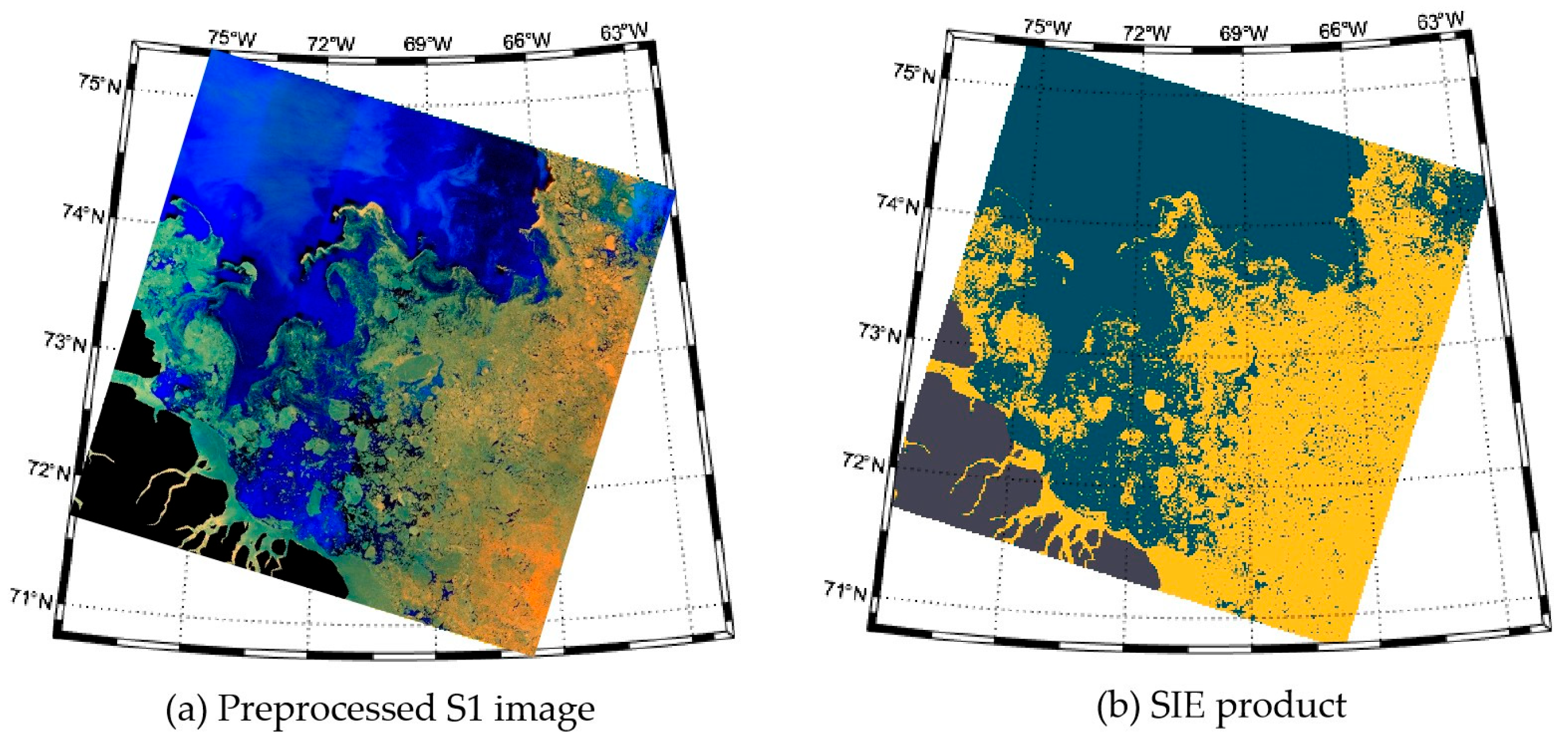
Figure 1. Example of a preprocessed S1 image and the corresponding SIE product. (a) shows the preprocessed S1 image. (b) presents the corresponding SIE product, where yellow denotes sea ice, cyan indicates open water, and dark gray represents land.
Remotesensing 17 03166 g001
Figure 2. Monthly distribution and proportion of SIE products from 2020 to 2023. The broken line indicates the monthly variation in product proportion.
Remotesensing 17 03166 g002
Figure 3. Flowchart of SIE product generation. The workflow includes image preprocessing, SIE extraction based on an integrated stacking U-Net algorithm, and the generation of the final SIE product.
Remotesensing 17 03166 g003
Figure 4. Comparison of S1 and AMSR2 products from 2020 to 2023. The blue and yellow lines show the AMSR2 and S1 SIC, respectively, while the red line indicates their mean absolute difference.
Remotesensing 17 03166 g004
Figure 5. Scatterplot of S1 SIC versus AMSR2 SIC, with data points mainly distributed along the one-to-one line, showing good consistency. The red dashed line represents the one-to-one line, where the S1-derived SIC and AMSR2 SIC are equal.
Remotesensing 17 03166 g005
Figure 6. Trend of monthly mean absolute differences between the S1 and AMSR2 products. The average differences are notably higher in May, June, July, and August.
Remotesensing 17 03166 g006
Figure 7. Spatial distribution of the center points of image-level mean absolute differences between S1 products and AMSR2 products during May–August from 2020 to 2023. Blue indicates differences of 0–10%, green indicates 10–20%, yellow indicates 20–30%, orange indicates 30–40%, and red indicates differences greater than 40%. The red dashed ellipse indicates the regions of high difference.
Remotesensing 17 03166 g007
Figure 8. Case study over the eastern Chukchi Sea on August 28, 2020. Panels (ac) show S1 images acquired on 27 August (S1B), 28 August (S1A, primary scene for analysis), and 29 August (S1B), respectively. Panels (df) present the corresponding S1 SIE product, the SIC converted from the SIE, and the reference AMSR2 SIC product for the scene shown in (b). The image-averaged difference between the S1 and AMSR2 SIC is 12%. Arrows denote variations over time, while the rectangles highlight identical regions of specific interest.
Remotesensing 17 03166 g008
Figure 9. Case study over the Chukchi Sea on 7 August 2020. Panels (ac) show S1 images acquired on 6 August (S1A), 7 August (S1B, primary scene for analysis), and 10 August (S1B), respectively. Panels (df) present the corresponding S1 SIE product, the SIC converted from the SIE, and the reference AMSR2 SIC product for the scene shown in (b). The image-averaged difference between the S1 and AMSR2 SIC is 22%. Arrows denote variations over time, while the rectangles highlight identical regions of specific interest.
Remotesensing 17 03166 g009
Figure 10. Case study over the transition zone between the Chukchi Sea and the East Siberian Sea on 15 August 2020. Panels (ac) show S1 images acquired on 14 August (S1B), 15 August (S1A, primary scene for analysis), and 16 August (S1B), respectively. Panels (df) present the corresponding S1 SIE product, the SIC converted from the SIE, and the reference AMSR2 SIC product for the scene shown in (b). The image-averaged difference between the S1 and AMSR2 SIC is 47%. Arrows denote variations over time, while the rectangles highlight identical regions of specific interest.
Remotesensing 17 03166 g010
Figure 11. Image captured near the central Arctic region north of the Chukchi Sea on 10 July 2020. (a) Image acquired by S1B; (b) S1 SIE product; (c) S1 SIC product; (d) AMSR2 SIC product. The image-averaged difference between the S1 and AMSR2 SIC is 59%.
Remotesensing 17 03166 g011
Figure 12. Visualization of Sentinel-1C SIE products. Images (a,b) represent high SIC regions, while the images (ch) depict the marginal ice zone. All images are acquired during the melt seasons (May–July 2025).
Remotesensing 17 03166 g012
Figure 13. Monthly and average Integrated Index values for all sub-models in 2020. The highlighted sections indicate the sub-model with the lowest Integrated Index each month, representing the highest contribution to the ensemble.
Remotesensing 17 03166 g013
Figure 14. Two components of the Integrated Index for all sub-models by month in 2020. For each sub-model, the left column represents the difference from the ensemble result (1–DSC_with_integrated_result), and the right column shows the mean DSC with the other sub-models (mean_pairwise_DSC).
Remotesensing 17 03166 g014
Figure 15. Example cases of high-error scenes in regions with high SIC. Panels (a,b) show the corresponding SIE products along with the extraction results from each sub-model.
Remotesensing 17 03166 g015
Table 1. List of variables and their descriptions in the SIE products.
No.VariablesDescriptions
1LongitudeLongitude of each sea ice and land mask record
2LatitudeLatitude of each sea ice and land mask record
3SeaIce0 denotes open water, and 1 denotes sea ice
4Mask0 indicates no land, and 1 indicates land
Disclaimer/Publisher’s Note: The statements, opinions and data contained in all publications are solely those of the individual author(s) and contributor(s) and not of MDPI and/or the editor(s). MDPI and/or the editor(s) disclaim responsibility for any injury to people or property resulting from any ideas, methods, instructions or products referred to in the content.