Highlights
What are the main findings?
- A Transformer-based model for 8-fold tropical cyclone wind field downscaling is developed.
- A novel TC dataset is constructed by integrating ERA5 reanalysis data with Cyclobs satellite observations.
What is the implication of the main finding?
- The method outperforms baselines in RMSE and dynamical metrics, and accurately reconstructs fine-scale tropical cyclone wind structures.
Abstract
Tropical cyclones (TCs) rank among the most destructive natural hazards globally, with core damaging potential originating from regions of intense wind shear and steep wind speed gradients within the eyewall and spiral rainbands. Accurately characterizing these fine-scale structural features is therefore critical for understanding TC intensity evolution, wind hazard distribution, and disaster mitigation. Recently, the deep learning-based downscaling methods have shown significant advantages in efficiently obtaining high-resolution wind field distributions. However, existing methods are mainly used to downscale general wind fields, and research on downscaling extreme wind field events remains limited. There are two main difficulties in downscaling TC wind fields. The first one is that high-quality datasets for TC wind fields are scarce; the other is that general deep learning frameworks lack the ability to capture the dynamic characteristics of TCs. Consequently, this study proposes a novel deep learning framework, CycloneWind, for downscaling TC surface wind fields: (1) a high-quality dataset is constructed by integrating Cyclobs satellite observations with ERA5 reanalysis data, incorporating auxiliary variables like low cloud cover, surface pressure, and top-of-atmosphere incident solar radiation; (2) we propose CycloneWind, a dynamically constrained Transformer-based architecture incorporating three wind field dynamical operators, along with a wind dynamics-constrained loss function formulated to enforce consistency in wind divergence and vorticity; (3) an Adaptive Dynamics-Guided Block (ADGB) is designed to explicitly encode TC rotational dynamics using wind shear detection and wind vortex diffusion operators; (4) Filtering Transformer Layers (FTLs) with high-frequency filtering operators are used for modeling wind field small-scale details. Experimental results demonstrate that CycloneWind successfully achieves an 8-fold spatial resolution reconstruction in TC regions. Compared to the best-performing baseline model, CycloneWind reduces the Root Mean Square Error (RMSE) for the U and V wind components by 9.6% and 4.9%, respectively. More significantly, it achieves substantial improvements of 23.0%, 22.6%, and 20.5% in key dynamical metrics such as divergence difference, vorticity difference, and direction cosine dissimilarity.
1. Introduction
Tropical cyclones (TCs) are intense rotating storm systems that originate over warm tropical oceans, characterized by low-pressure centers and closed low-level circulation. These systems inflict devastating impacts through torrential rain, destructive storm surges, and extreme winds. High-resolution (HR) wind field data containing fine-scale wind structures, particularly eyewalls and steep radial gradients, are critical to forecast the evolution of the TC intensity, simulate the dynamics of storm surges, and quantify disaster risks. Although these data could be obtained through satellite observations such as the scatterometer [1] and altimeter [2], they suffer from temporal discontinuity and orbital coverage gaps, hindering the continuous dynamical analysis of the TC cores. Meanwhile, reanalysis data that deliver globally consistent, hourly atmospheric states through advanced data assimilation are often used together with satellite observations for analyzing TC dynamics. However, even the latest ERA5 [3,4] has insufficient resolution to resolve the maximum wind speeds, vortex-scale dynamics governing TC intensification, or other critical kilometer-scale sub-mesoscale features. Therefore, the downscaling methodologies are considered for transforming accessible low-resolution (LR) meteorological model outputs into high-fidelity kilometer-scale wind fields while rigorously preserving the complex nonlinear dynamics of TC systems.
Traditional meteorological downscaling methods are typically categorized into two types: dynamical and statistical downscaling. Dynamical downscaling [5,6,7,8,9] uses physical principles, relying on Global Climate Models or reanalysis data to drive Regional Climate Models over limited areas. However, it requires significant computational resources, struggles with long-term simulations, and produces outputs with systematic errors due to atmospheric complexity. Statistical downscaling [10,11,12,13], in contrast, is computationally efficient and flexible, linking large-scale climate factors to localized meteorological variables through statistical models. Although it partially mitigates systematic GCM biases, traditional statistical methods lack the complexity to fully capture weather system intricacies, leading to reduced accuracy in simulated outcomes.
In recent years, deep learning methods have emerged as robust nonlinear statistical modeling tools with considerable potential in meteorological downscaling, offering superior performance and computational efficiency. Early research primarily adapted computer vision super-resolution models to meteorological downscaling. Among these, DeepSD [14] pioneered the application of the SRCNN architecture, demonstrating superior performance relative to traditional statistical methods and providing crucial validation for deep learning feasibility in meteorological downscaling. Subsequently, recognizing significant spatial correlations among meteorological elements, researchers identify attention mechanisms as a promising development direction. To effectively integrate digital elevation model data into the downscaling process, Shen et al. [15] and Liu et al. [16] proposed a cross-attention mechanism and a terrain-guided attention module, respectively, achieving kilometer-scale surface temperature reconstruction. Furthermore, Wang et al. [17] introduced dynamic and hierarchical attention modules to adaptively guide multiscale mapping relationship learning in meteorological data. Building on Transformer breakthroughs in computer vision tasks, Nguyen et al. [18] established the first Transformer-based foundation model for weather and climate science. Its inherently flexible and scalable architecture supports multitask learning, providing a unified framework for meteorological downscaling. In addition, Ling et al. [19] developed a probabilistic downscaling framework using diffusion models to quantify downscaling process uncertainty, which successfully reconstructs a 180-year historical climate sequence for East Asia. This demonstrates the potential of diffusion models to generate high-fidelity meteorological fields with quantifiable uncertainty. Collectively, these studies underscore the significant advantages conferred by deep learning models, including convolutional neural networks, attention mechanisms, Transformers, and diffusion models in revolutionizing meteorological downscaling tasks.
Wind field downscaling represents a critical component of meteorological downscaling research [20,21,22,23]. Relative to parameters such as temperature and salinity, near-surface wind fields exhibit stronger spatiotemporal variability and more complex local forcing responses. These characteristics significantly increase downscaling uncertainty and necessitate models with enhanced representational capacity. To address the dynamic influence of complex terrain, researchers have developed modules integrating terrain features to enhance downscaling accuracy. For instance, Zhong et al. [24] employed a UFormer architecture incorporating a dedicated HR terrain data encoder. Yu et al. [25] proposed a terrain-guided flat memory network and design an enhanced terrain-guided loss function utilizing HR remote sensing data. Sekiyama et al. [26] introduced an SRCNN variant featuring separate encoders for wind and terrain data, employing ensemble models trained with varying random seeds for kilometer-scale downscaling across Japan’s main island region. Subsequently, Lian et al. [27] developed the TerraWind model, which combines terrain factors and station-to-station relationships to capture multiscale wind–terrain correlations. Concurrently, other studies have explored efficient modules and innovative model architectures. For example, Liu et al. [28] enhanced multiscale feature fusion by introducing a dual-cross-attention mechanism within a UNet architecture. Mardani et al. [29] applied generative diffusion models, combining UNet mean prediction with diffusion models’ residual correction to achieve 2 km scale downscaling throughout the Taiwan region. These approaches primarily target either background wind fields or general weather systems over land under complex terrain conditions. Conversely, research addressing marine wind fields, especially extreme wind fields associated with strong weather systems, remains relatively limited. This limitation impedes understanding and prediction of TC wind field characteristics in critical air–sea interaction zones.
In this study, we focus on downscaling extreme sea surface wind field in TC scenarios, a type of intense weather system characterized by unique dynamical structures. TC wind fields exhibit distinct nonlinear structural features, including sharp wind speed gradients, strong rotational characteristics, and concentrated maximum winds. These complex dynamical characteristics and fine-scale spatial patterns differ fundamentally from terrestrial wind fields or general weather systems. Consequently, generalized wind field downscaling models developed for typical scenarios encounter substantial limitations when applied to TCs, failing to effectively represent unique TC structures and dynamical processes, particularly steep gradients and vortical features. Moreover, when processing extreme wind speeds and complex TC structures, these models exhibit substantially reduced predictive accuracy, frequently producing excessively smoothed outputs with structural distortions. Therefore, incorporating unique dynamical structures, dynamical constraints, and extreme characteristics into deep learning frameworks constitutes a fundamental challenge for achieving HR reconstruction. To address these challenges, we introduce a dynamics-constrained deep learning model for TC wind field downscaling using satellite observations. The major contributions are as follows:
(1) We construct a high-quality TC dataset by integrating Cyclobs satellite observations with ERA5 reanalysis data. Following grid interpolation and spatiotemporal matching, this dataset supports 8 × spatial downscaling of sea surface wind fields, with explicit coverage of critical TC structures, including TC eyewalls and spiral rainbands. To enhance feature representation, we further incorporate low cloud cover, surface pressure, and top-of-atmosphere incident solar radiation as auxiliary atmospheric variables in our LR input.
(2) We propose a Transformer-based TC wind field downscaling framework, CycloneWind, incorporating three specialized wind field dynamical operators with the ability to capture multiscale TC dynamics, and a dynamics-constrained loss function is formulated based on divergence and vorticity domains to enforce wind field dynamical consistency.
(3) Within the CycloneWind framework, the Adaptive Dynamics-Guided Block (ADGB) is designed to parallelly leverage the wind shear detection operator and wind vortex diffusion operator. Specifically, the wind shear detection operator is used to extract horizontal momentum transitions by leveraging gradient computation concepts similar to the Sobel operator; and the vortex diffusion operator is responsible for quantifying kinetic energy dispersion and concentration within vortex cores through second-order differentiation mechanisms inspired by Laplace operators. Crucially, the parallel structure establishes a fusion convolution that dynamically weights operator outputs according to TC evolution stages.
(4) In order to combine global dependency modeling with local spectral feature extraction, the Filtering Transformer Layers (FTLs) are introduced to embed high-frequency filtering operators directly within Transformer blocks. This capability specifically addresses the inherent limitations of ERA5 reanalysis data in high-wind-speed regions, where coarse spatial resolution obscures sharp velocity gradients and sub-scale vorticity features. The injected high-frequency components compensate for spectral energy loss during downscaling, enhancing reconstruction fidelity in diagnostically critical zones.
(5) Comprehensive experiments are conducted to evaluate the performance of CycloneWind compared with general deep learning frameworks. Firstly, quantitative performance analysis employs RMSE and specialized wind dynamical metrics, DivDiff, VorDiff, and CosDis, to holistically assess wind field reconstruction accuracy. Subsequently, systematic ablation studies isolate contributions of core modules and LR auxiliary atmospheric inputs, establishing effectiveness in modules and additional input. Finally, visualization integrates wind vector fields, divergence–vorticity diagrams, and bias maps, validating fine-scale structural preservation in critical regions.
The remainder of this paper is organized as follows: Section 2 describes the ERA5 reanalysis data sources, Cyclobs TC data sources, and data processing procedures. Section 3 details the proposed downscaling framework CycloneWind, including its overview architecture, wind field dynamical operators, ADGBs, FTLs, and the wind dynamics-constrained loss function. Section 4 specifies implementation details, evaluation metrics, and baseline methods. Section 5 gives experimental results, an ablation study on the modules and input elements, and wind speed analysis. Finally, Section 6 concludes the paper.
2. Datasets
This study utilizes two distinct data sources to build our TC wind field datasets: (1) ERA5 hourly reanalysis data on single levels, serving as the model LR input, and (2) Cyclobs TC satellite observation data, employed as the HR ground truth. The details of these data and data processing procedures are as follows.
2.1. ERA5 Data
The ERA5 data constitute the fifth-generation global atmospheric reanalysis produced by the European Center for Medium-Range Weather Forecast (ECMWF). Utilizing an advanced four-dimensional variational data assimilation system, it synthesizes historical global observations with numerical model forecasts to generate high-quality atmospheric state estimates spanning from 1940 to the present. In our study, we extract the following five meteorological variables at 0.25° × 0.25° spatial resolution and 1-h temporal resolution: 10 m u-component of wind, 10 m v-component of wind, low cloud cover, surface pressure, and top-of-atmosphere incident solar radiation.
2.2. Cyclobs Data
The Cyclobs TC satellite observation datasets are derived from the Cyclobs Level-2 wind product developed by the French Research Institute for Exploitation of the Sea (IFREMER). This product utilizes C-band synthetic aperture radars (SARs) aboard the Sentinel-1A and Sentinel-1B satellites to generate a dedicated TC dataset with a spatial resolution of 0.01° × 0.01°. To mitigate the known underestimation of extreme winds in SAR retrievals caused by factors such as rainband contamination, high-wind saturation, and viewing geometry effects, the Cyclobs Level-2 wind product incorporates dual-polarization signals, specifically both VV and VH, from Sentinel-1 SAR acquisitions. While VV-polarized backscatter loses sensitivity at extreme wind speeds, cross-polarized VH signals remain highly sensitive [30]. The wind product further combines these SAR measurements with a priori wind information from ECMWF to enhance accuracy, and allows high-resolution mapping of wind variability within and around TC eyes [31].
In this study, the Cyclobs data include all named TC events over major global ocean basins from 2017 to 2022, covering the full lifecycle stages of TCs, including genesis, development, maturity, and decay. The kilometer-scale spatial resolution enables clear resolution and precise capture of key dynamical structures in TCs, providing an essential observational basis for investigating convective mechanisms and intensity evolution. It is important to note that, due to constraints inherent in satellite observation principles, this dataset is exclusively available over open ocean areas, and terrestrial regions are uniformly assigned null values.
2.3. Data Processing
Critical data processing steps ensure grid alignment and data validity between the ERA5 reanalysis data and Cyclobs observations data, establishing the foundation for efficient and reliable wind field downscaling. First, rigorous quality control is performed to screen raw Cyclobs TC observation data, eliminating cases severely affected by observational conditions or land interference with substantial data gaps, while ensuring selected samples retain the complete TC structure characteristics. Subsequently, spatiotemporal alignment between LR and HR data is conducted. To reduce model complexity, computational costs, and training difficulty, the downscaling target factor is adjusted from 25-fold to a more achievable 8-fold. To accomplish this goal and ensure precise spatiotemporal matching, we first temporally interpolate the hourly ERA5 data to match the exact timestamps of the Cyclobs observations using bicubic interpolation. Then, the Cyclobs data at 1 km spatial resolution are spatially regridded to a 3.125 km resolution using nearest-neighbor interpolation. It should be noted that during the spatial interpolation process, the target latitude–longitude grid with a spatial resolution of 3.125 km must correspond to the ERA5 latitude–longitude grid, which has a spatial resolution of 25 km. The final spatiotemporally matched dataset is used for training and evaluating the typhoon wind field downscaling model.
3. Method
3.1. Problem Formulation
In wind downscaling studies, the wind field can be orthogonally decomposed into zonal wind speed u and meridional wind speed v to preserve its vector properties. In this paper, we incorporate additional atmospheric elements as multivariate model input, enhancing the accuracy and reliability of the downscaling process. Specifically, the input variables consist of wind field and auxiliary atmospheric variables , including low cloud cover (LCC), surface pressure (SP), and top-of-atmosphere incident solar radiation (TISR). Utilizing deep learning methods, the downscaling model learns the complex mapping relationship from the LR multivariate meteorological elements to the target HR wind field , with the objective of minimizing the discrepancy against HR ground truth observations . The downscaling process can be mathematically expressed as
Here, f represents a mapping function parameterized by , denotes the loss function, and s is the downscaling factor. The LR input is gridded at resolution, while the corresponding HR output is gridded at resolution, both covering a km spatial domain, which is sufficient to encompass typical TC areas.
3.2. Overall Architecture
This subsection delineates the overall architecture of the CycloneWind model, with structural details illustrated in Figure 1. Leveraging Sobel and Laplace operators, we initially introduce three wind field dynamical operators. The CNN-based ADGB integrates wind shear detection and wind vortex diffusion operators for TC feature enhancement, and the FTLs employ high-frequency filtering operators to resolve sub-grid turbulent structures. Sequentially cascading one ADGB, three FTLs, and residual connections constitutes the Dynamics-Guided Hybrid Module (DGHM). Furthermore, we formulate a wind dynamics-constrained loss function enforcing dynamical consistency through divergence and vorticity domain transformations.
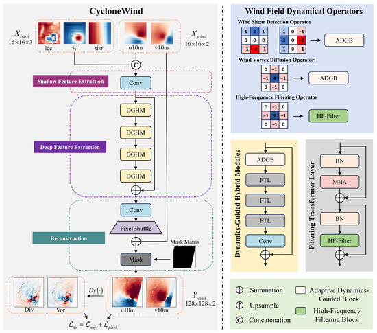
Figure 1.
Architecture of the proposed CycloneWind framework. The model incorporates three specialized wind field dynamical operators within four Dynamics-Guided Hybrid Modules (DGHMs), which consist of an Adaptive Dynamics-Guided Block (ADGB) and three Filtering Transformer Layers (FTLs). A dynamics-constrained loss function enforces fluid dynamical consistency across the network.
3.3. Wind Field Dynamical Operators
We implement classical operators, the Sobel operator, the Laplace operator and the modified Laplace operator, with wind dynamics-inspired names to advance structure detection and high-frequency information enhancement in TC wind fields. These specialized operators include
- (1)
- Wind Shear Detection Operator
The wind shear detection operators and , constructed based on the Sobel operators, quantitatively characterize the horizontal wind shear intensity by computing the spatial gradient tensors of the zonal u and meridional v components. Physically, positive gradient zones indicate downwind acceleration corridors, while negative zones mark upwind deceleration belts, with this sign signature serving as a critical diagnostic for TC dynamical structures. Through domain-wide wind shear field computation, these operators resolve multiscale dynamical boundaries in tropical cyclones, including eyewall boundaries and spiral rainbands.
- (2)
- Wind Vortex Diffusion Operator
The wind vortex diffusion operator adapts the Laplace operator into a second-order differential formulation applied directly to the wind speed field. Physically, this operator describes the diffusion or concentration of kinetic energy associated with vortex cores, rather than directly quantifying turbulent kinetic energy or energy flux. Positive values indicate the outward diffusion of kinetic energy from the central region of the vortex, while negative values signify its inward concentration toward the core. This diffusion signature pinpoints critical structural features: local extrema identify the primary vortex core boundary and secondary circulation centers, while steep gradients highlight dynamic transition zones, particularly the radius of maximum winds.
- (3)
- High-Frequency Filtering operator
The high-frequency filtering operator employs a modified Laplace operator by reconstructing its discrete formulation through enhanced weighting coefficients at the central grid. Compared to the wind vortex diffusion operator , this operator increases the operator’s sensitivity to atmospheric high-frequency features, enabling more effective capture of key dynamical characteristics at vortex core boundaries.
3.4. Adaptive Dynamics Guided Blocks
Wind shear and turbulent kinetic energy diffusion represent key kinematic characteristics governing tropical cyclone (TC) intensity evolution and structural organization. These observable features are valuable for detecting structural asymmetries, rainbands, eyewall boundaries, and environmental interaction zones. Specifically, fine-scale analysis of horizontal wind shear structures in the TC periphery enables the detection of circulation boundaries and potential outer rainbands. Concurrently, spatial distributions of wind vortex diffusion coefficients quantify turbulent mixing intensity, serving as effective indicators for precisely delineating typhoon eye boundaries. To explicitly incorporate these dynamical constraints within the downscaling framework, we introduce ADGBs as illustrated in Figure 2. These blocks are augmented with two specialized operators: the wind shear detection operator extracts zonal and meridional gradient variations to capture divergence and vorticity signatures, and the wind vortex diffusion operator targets high-frequency central regions characterized. Together, they form an adaptive feature extraction and fusion mechanism that dynamically integrates these wind field characteristics to selectively reinforce dynamical consistency within the main network’s predictions. Mathematically, this fusion process is expressed as
where and denote the input and output feature map, and denote the wind shear detection operator, denotes the wind vortex diffusion operators, and denotes convolution with kernels and with kernels.
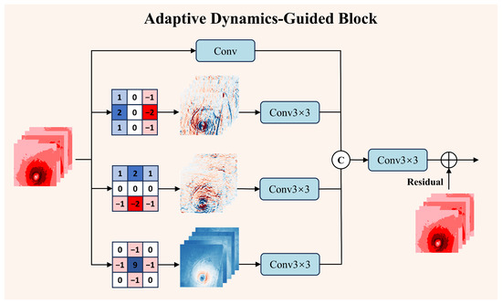
Figure 2.
Architecture of the Adaptive Dynamics-Guided Block. The Block processes wind field inputs through the wind shear detection operator and wind vortex diffusion operator. Outputs from all branches undergo adaptive feature fusion via a convolutional layer.
3.5. Filtering Transformer Layers
Transformers typically demonstrate superior capability to CNNs in capturing long-range dependencies while mitigating the over-smoothing effects that can occur in CNN-based local feature processing, particularly within high-wind-speed zones of TCs. Consequently, we employ a Swin Transformer-based architecture where the self-attention mechanism effectively models global feature relationships. For input features , the self-attention mechanism computes
where , , and are learnable projection matrices for the query Q, key K, and value V, respectively. Multi-head attention extends this across h subspaces:
High-frequency components in wind fields are critical for resolving fine-scale dynamic structures such as eyewall boundaries and small-scale vortices within TCs. To explicitly preserve these features, we utilize a high-frequency filtering operator that extracts multiscale high-frequency signatures. This operator is integrated with convolutional layers to form a high-frequency filtering block, replacing the standard feed-forward network. The block is formulated as
where denotes a 3 × 3 kernel convolution and represents the high-frequency filtering operator. The FTLs synergistically combine global dependency modeling with localized high-frequency feature extraction, significantly enhancing the reconstruction of critical fine-scale details. The FTLs can be defined by
Here, indicates a normalization method, and we implement the BatchNorm method in this study.
3.6. Wind Dynamics-Constrained Loss Function
Divergence and vorticity are two fundamental dynamical quantities in TC wind fields. Divergence describes the degree of horizontal air radiation or convergence, directly impacting vertical motion and weather system development. Vorticity measures the tendency of air to rotate around a vertical axis, representing the rotational characteristics essential to weather systems, especially core features like TC eyewalls and cyclonic circulations. Let and represent the zonal and meridional wind speed, respectively. Divergence and vorticity are mathematically expressed as
Incorporating divergence and vorticity as dynamical constraints into the loss function guides deep learning models to respect atmospheric dynamics. This improves dynamical consistency in wind field downscaling by aligning them with HR references in both statistics and key dynamical mechanisms. This approach mitigates dynamically unreasonable artifacts and improves the interpretability and reliability. The wind dynamics-constrained loss function is expressed as
Here, and represent the downscaling model output and HR ground truth, respectively. The loss functions comprise for pixel-wise reconstruction loss, and and for divergence and voracity domain constraints, with relative weighting controlled by .
4. Experiments
4.1. Implementation Details
In our study, we employ a five-fold cross-validation strategy, a widely recognized methodology adopted across multiple scientific domains [32,33,34], to enhance the validity and generalization of our experimental results. This approach is particularly crucial given the inherent scarcity of high-quality tropical cyclone observations. To maximize the utilization of all available samples and ensure comprehensive coverage of diverse TC cases, the full dataset comprising 1203 samples is used. The dataset is randomly partitioned into five mutually exclusive folds. In each iteration, one fold serves as the validation set, while the remaining four are used for training, corresponding to a 4:1 ratio between training and validation sets. This process is repeated five times such that each fold is used exactly once as the validation set, thereby enabling a robust and comprehensive evaluation of the model’s performance.
Notably, although the TC wind field dataset contains temporal information, we deliberately avoid chronological partitioning strategies. This decision stems from the limited relevance of temporal splits for evaluating our core wind field downscaling model. The model’s primary objective is learning underlying dynamical relationships within the data rather than forecasting specific future TC states. Chronological partitioning could introduce temporal biases and reduce the effective sample size, which our cross-validation strategy successfully mitigates.
During our training process, the input LR training data consist of 16 × 16 grids, while the corresponding target HR data comprise 128 × 128 grids. Our model is configured with 256 feature channels and trained for 50,000 iterations using a batch size of 32. Optimization is performed with the Adam optimizer at a learning rate of . All experiments are conducted on an NVIDIA GeForce RTX 3090 GPU (Lenovo, Beijing, China).
4.2. Evaluation Metrics
In this subsection, we systematically introduce the standardized evaluation metric Root Mean Squared Error (RMSE) and a dynamics-based evaluation metrics (DivDiff, VorDiff, CosDis) to establish a multidimensional quantitative assessment system for model performance. The RMSE metric quantifies the overall deviation magnitude between predictions and observations by computing root mean squared differences, thereby objectively evaluating the model’s comprehensive accuracy. Specifically, for each timestamp t, we define the predicted HR wind field as and the corresponding HR observation as . The mathematical expressions are as follows:
Here, denotes L2 norm. In wind field dynamical analysis, divergence and vorticity serve as core dynamical quantities characterizing the convergence and divergence properties and fluid rotational characteristics of wind fields, respectively, while wind direction defines the spatial orientation of wind velocity vectors. To quantitatively assess the model’s capability in restoring wind field dynamical principles, this study employs three specialized metrics: wind divergence difference, DivDiff, wind vorticity difference, VorDiff, and wind direction cosine dissimilarity, CosDis. These are formally defined as follows:
For RMSE, DivDiff, VorDiff, and CosDis, smaller values indicate better model performance.
4.3. Comparison Methods
We select four representative deep learning models from the image super-resolution domain as primary benchmarks, including EDSR [35], RCAN [36], SwinIR [37], and SRNO [38], to comprehensively evaluate the performance of our proposed CycloneWind. These models collectively encompass diverse technical pathways in super-resolution research: EDSR serves as a classic CNN-based residual network that demonstrates the effectiveness of simplified architecture and stacked residual blocks, providing a strong baseline for deep CNN architectures with demonstrated strong feature extraction capabilities; RCAN introduces channel attention mechanisms to adaptively weight informative feature channels, representing a flagship model for attention mechanisms in super-resolution that can selectively emphasize informative features; SwinIR adapts the Swin Transformer architecture to leverage shifted window and self-attention mechanisms for capturing global dependencies, serving as a leading representative of Transformer-based vision models; and SRNO employs neural operators to learn continuous mappings between function spaces, offering a novel modeling perspective that operates beyond conventional discretized grid-based approaches. Collectively, this strategically selected set of benchmarks represents major contemporary super-resolution paradigms, enabling a rigorous evaluation of CycloneWind against foundational deep learning approaches.
5. Results
5.1. Experiment Results
This subsection presents a quantitative model comparison on the TC wind field dataset using RMSE, DivDiff, VorDiff, and CosDis metrics, with comprehensive results detailed in Table 1. For equitable comparison with baseline models such as EDSR, RCAN, SwinIR, and SRNO, our CycloneWind includes configurations both with and without the wind dynamics-constrained loss functions (dyloss). Among the baseline models, EDSR exhibits the maximal error, RCAN demonstrates moderate performance gains over EDSR, SRNO shows slightly elevated RMSE but achieves some improvements on dynamics-based metrics, and SwinIR delivers comparatively robust performance. Without dyloss, CycloneWind already outperforms all baselines, achieving significant RMSE reductions relative to the suboptimal model: 8.8% reduction for zonal wind speed RMSE-U, 6.8% reduction for meridional wind speed RMSE-V, and 9.0% reduction for overall wind speed RMSE-Speed. More significantly, it exhibits substantial gains in dynamical fidelity: DivDiff decreases by 16.2%, VorDiff by 15.8%, and CosDis by 17.9%. This pronounced dynamical superiority proves more critical than point-wise error reductions, as dynamically consistent reconstructions are paramount for meteorological applications. Integrating dyloss yields further enhancement. Compared to its version without dyloss, CycloneWind with dyloss achieves an additional 8.2% reduction in DivDiff, 8.0% in VorDiff, and 3.1% in CosDis. These dynamics-based metrics are vital for maintaining structurally consistent wind field reconstructions. Consequently, the complete CycloneWind model (with dyloss) achieves significant error reductions: 9.6% in RMSE-U, 4.9% in RMSE-V, and 8.5% in RMSE-Speed, alongside substantial improvements of 23.0% in DivDiff, 22.6% in VorDiff, and 20.5% in CosDis, demonstrating clear superiority under this multifaceted evaluation.

Table 1.
Overall performance of the proposed model and other methods in RMSE-U, RMSE-V, RMSE-Speed, DivDiff, VorDiff, and CosDis. Bold text denotes the best performance, while underlined text denotes the second best.
5.2. Case Study
This subsection provides a detailed visual evaluation through representative case studies, crucial for understanding model performance on complex real-world scenarios. Five TC cases spanning different years are randomly selected from the five-fold cross-validation set: TC MARIA on 23 September 2017 at 10:44:51 UTC, TC HECTOR on 10 August 2018 at 16:57:14 UTC, TC HAGIBIS on 8 October 2019 at 20:31:45 UTC, TC MARIE on 3 October 2020 at 14:20:24 UTC, and TC MINDULLE on 25 September 2021 at 20:49:58 UTC.
Qualitative assessments rigorously compare HR ground truth against reconstructions from four established super-resolution architectures and our CycloneWind model. To holistically evaluate dynamical fidelity and pinpoint spatial discrepancies, we explicitly visualize spatial error distributions through bias maps integrated into all visual comparisons. Further analyses supplement these with wind speed and wind direction arrow plots, as shown in Figure 3, and spatial visualizations of divergence and vorticity fields, as shown in Figure 4 and Figure 5. This integrated multidynamics visualization framework provides comprehensive insights into model performance across fundamental atmospheric dynamics.
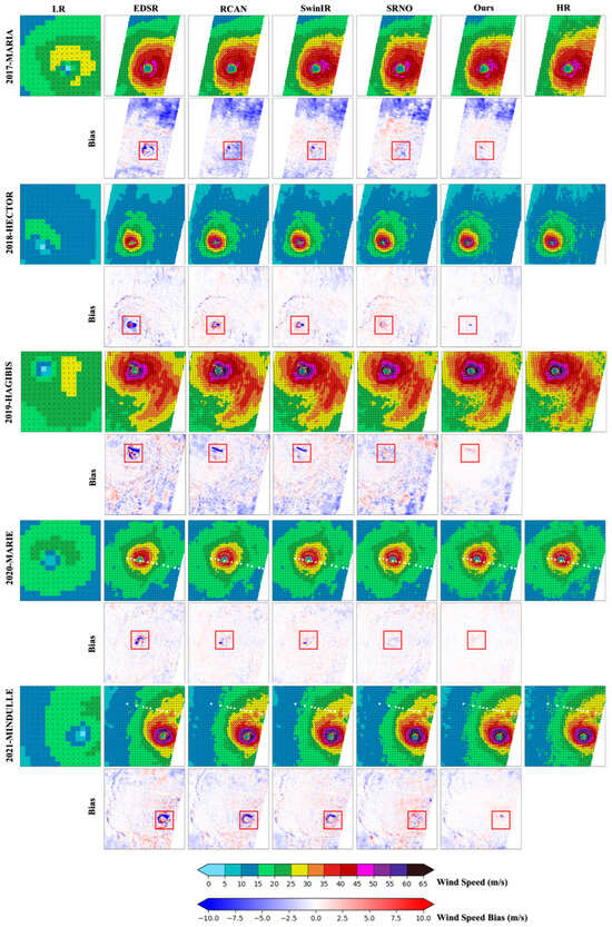
Figure 3.
Diagnostic comparison and error distribution of downscaled TC wind fields between downscaling results and ground truth. Red frames highlight regions of substantial inter-model error differences.
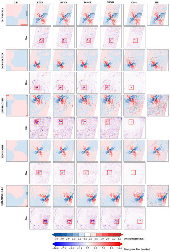
Figure 4.
Diagnostic comparison and error distribution of downscaled TC divergence fields between downscaling results and ground truth. Red frames highlight regions of substantial inter-model error differences.
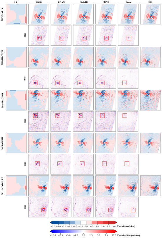
Figure 5.
Diagnostic comparison and error distribution of downscaled TC vorticity fields between downscaling results and ground truth. Red frames highlight regions of substantial inter-model error differences.
To enable a more intuitive observation of inter-model differences, particularly in the critical regions of the typhoon eye, eyewall, and adjacent areas where model capabilities are most challenged by intense winds and sharp gradients, we highlight these regions with red boxes in all figures. Results consistently demonstrate that within these highlighted areas, CycloneWind exhibits superior clarity, accuracy, and structural integrity compared to all benchmark models. Crucially, the bias maps within these red boxes reveal significantly smaller errors for CycloneWind, clearly accentuating its performance advantages where they matter most.
5.3. Ablation Study on Modules
To validate the effectiveness and necessity of the core components and loss function in the proposed CycloneWind model, systematic ablation studies are conducted. Using the complete model as the baseline, we sequentially remove the dynamics-constrained loss function (dyloss), replaced the high-pass filtering convolution in FTLs with standard MLP layers, and finally eliminated the ADGBs. As shown in Table 2, removing dyloss slightly increased numerical errors with 0.8% higher RMSE-U and 1.1% lower RMSE-V, but substantially degraded dynamical consistency metrics by elevating DivDiff 9.4% and VorDiff 8.7%. This demonstrates its critical role in enforcing dynamically meaningful solutions despite minor point-wise accuracy trade-offs. Removing the high-pass filtering block from the FTL leads to a comprehensive performance decline, with significant increases observed across all metrics: RMSE-U, RMSE-V, DivDiff, and VorDiff increase by 6.3%, 6.7%, 9.8%, and 10.0%, respectively. Removing the ADGBs induces the most severe deterioration, with the largest increases in errors with corresponding increases of 13.2%, 12.4%, 11.6%, and 12.7% in these metrics. These results indicate that while the dynamics-constrained loss function entails a minor compromise in numerical accuracy, it delivers substantial gains in dynamics-consistency metrics. Simultaneously, both the proposed ADGB and the FTL, particularly its high-pass filtering block, play indispensable roles within the model, as their removal or substitution significantly impairs its predictive capability.
Table 2.
Ablation study of proposed modules and loss function, including Adaptive Dynamics-Guided Blocks (ADGB), Filtering Transformer Layer (FTL), and wind dynamics-constrained loss (dyloss) in RMSE, DivDiff, VorDiff, and CosDis. Bold text denotes the best performance, while underlined text denotes the second best. The symbols ✓and ✗ denote the inclusion and exclusion of the module, respectively.
5.4. Ablation Study on Operators
To validate the effectiveness and necessity of the three wind field dynamical operators in the proposed CycloneWind model, systematic ablation studies were conducted. The baseline was established by removing all three dynamical operators from the CycloneWind model. Subsequently, we sequentially added the wind shear detection operator (WSDO), the wind vortex diffusion operator (WVDO), and the high-frequency filtering operator (HFFO). As shown in Table 3, incorporating WSDO led to a reduction of 0.2% in RMSE-U, 0.9% in RMSE-V, 0.4% in DivDiff, and 0.4% in VorDiff. In contrast, the addition of WVDO resulted in an increase of 0.4% in RMSE-U, but decreases of 0.6% in RMSE-V, 0.9% in DivDiff, and 0.4% in VorDiff. While the inclusion of WSDO and WVDO brought relatively modest overall improvements, HFFO contributed more significantly to model performance: its integration reduced RMSE-U by 1.7%, RMSE-V by 1.7%, DivDiff by 2.2%, and VorDiff by 2.1%. These results demonstrate that each of the three dynamical operators contributes to certain aspects of the model’s performance, with HFFO providing the most substantial gains.
Table 3.
Ablation study of proposed operators, including wind shear detection operator (WSDO), wind vortex diffusion operator (WVDO), and high-frequency filtering operator (HFFO). Bold text denotes the best performance, while underlined text denotes the second best. The symbols ✓and ✗ denote the inclusion and exclusion of the operator, respectively.
5.5. Ablation Study on Input Elements
To evaluate the contribution of LR auxiliary inputs to wind field downscaling, supplementary ablation experiments are conducted. We establish a baseline model utilizing only wind field elements as input. Building upon this baseline, three key meteorological variables, LCC, SP, and TISR, are systematically incorporated through individual and combined integrations. As shown in Table 4, Quantitative results demonstrate the dominant influence of LCC: its individual integration comprehensively improved performance, reducing RMSE-U by 3.78%, RMSE-V by 3.30%, DivDiff by 4.26%, and VorDiff by 3.73%. While SP and TISR showed marginal standalone contributions, their synergistic integration yielded measurable gains, decreasing the same metrics by 2.35%, 2.56%, 0.44%, and 0.86%. Collectively, integrating all three LR inputs (LCC+SP+TISR) achieves significant enhancements over the wind-only baseline, with 6.0% improvement in RMSE-U, 5.8% in RMSE-V, 4.7% in DivDiff, and 4.6% in VorDiff. These findings indicate that LCC is the critical factor for enhancing reconstruction accuracy, whereas SP and TISR, despite their limited individual effects, can synergistically optimize the wind field reconstruction process when combined.
Table 4.
Ablation study of input auxiliary elements, including low cloud cover (LCC), surface pressure (SP), and top-of-atmosphere incident solar radiation (TISR) in RMSE-U, RMSE-V, DivDiff, and VorDiff. Bold text denotes the best performance, while underlined text denotes the second best. The symbols ✓and ✗ denote the inclusion and exclusion of the element, respectively.
5.6. Wind Speed Study
In wind speed study, we classified wind fields into six formal categories according to the World Meteorological Organization TC scale to systematically evaluate the model’s performance robustness across meteorological intensities: Tropical Depression (10.8–17.1 m/s), Tropical Storm (17.1–24.4 m/s), Severe Tropical Storm (24.4–32.6 m/s), TC (32.6–41.4 m/s), Severe TC (41.4–51.9 m/s), and Super TC (≥51.9 m/s), with 0–10.8 m/s non-cyclonic conditions serving as the Normal Wind. As presented in Table 5, CycloneWind demonstrates significant advantages across all intensity regimes: it reduces RMSE by 6.0% in baseline conditions and by 7.4%, 10.5%, 9.6%, 5.6%, 3.4%, and 7.3% across the six cyclone categories, respectively. Remarkably, within the critical meteorological hazard range of Tropical Storm to Severe Tropical Storm, the model achieves an average error reduction of 10.05%, confirming its exceptional capacity for capturing developing cyclones. Notably, it maintains a substantial 7.3% improvement under destructive Super TC conditions, surpassing the extreme-condition performance of comparable models documented in existing literature, thereby validating its practical utility for disaster mitigation decision support systems.
Table 5.
Performance comparison of downscaling results against ground truth across meteorological wind speed classifications in RMSE. Bold text denotes the best performance, while underlined text denotes the second best.
6. Conclusions
This study successfully constructs and validates CycloneWind, a Transformer-based deep learning framework integrating wind field dynamical operators, aiming to achieve an 8-fold resolution downscaling of TC wind fields from 25 km to 3.125 km. The main works in our study are as follows:
(1) We first establish a high-quality dataset derived from Cyclobs satellite observations and ERA5 reanalysis data. Through comprehensive preprocessing involving grid interpolation and spatiotemporal matching, this dataset captures complete structural evolution across multiple TC intensity stages. The deliberate inclusion of low cloud cover, surface pressure, and top-of-atmosphere incident solar radiation as auxiliary variables significantly enriched multidimensional feature representation during downscaling.
(2) In our CycloneWind, we propose ADGBs to explicitly encode wind shear intensity and wind field rotational dynamics through synergistic integration of the wind shear detection operator and wind vortex diffusion operator. Then, we design FTLs by replacing SwinIR MLP blocks with high-frequency filtering operators alongside convolutional layers. Leveraging divergence and vorticity properties of TC wind fields, we formulate a divergence–vorticity composite loss function to enforce dynamical consistency in reconstruction.
(3) Through comprehensive experimental evaluation encompassing both quantitative metrics and qualitative analysis, CycloneWind demonstrates superior performance against publicly available super-resolution benchmark methods. In accuracy metrics, the model achieves significant RMSE reductions of 9.6%, 4.9%, and 8.5% for wind field in RMSE-U, RMSE-V, and RMSE-Speed, respectively. Regarding dynamical metrics, CycloneWind exhibits exceptional performance with 23.0%, 22.6%, and 20.5% reductions in DivDiff, VorDiff, and CosDis. These results conclusively demonstrate the enhanced dynamical consistency and rationality of the model in the generated output.
In summary, the CycloneWind framework provides a reliable and effective deep learning solution for high-precision downscaling of TC wind fields, notably achieving a successful fusion of dynamical operators and constraints to overcome limitations in purely data-driven models. It delivers significant improvements in both reconstruction accuracy and dynamics consistency, demonstrated by substantial enhancements across key quantitative metrics and dynamical statistical indicators. While focused on TCs, the framework exhibits strong generalization potential through its physically and dynamically aware mechanisms, including ADGBs, FTLs, and wind dynamics-constrained loss function, indicating applicability to downscaling broader meteorological elements like precipitation and temperature fields. This offers a novel technical pathway for advancing HR numerical weather prediction and refined analysis of severe weather events.
Author Contributions
Conceptualization, K.D., D.Z., X.S. and K.R.; Methodology, Y.H., K.D., Q.S., D.Z., X.S. and K.R.; Validation, Y.H., Q.S. and X.S.; Writing—original draft, Y.H.; Writing—review and editing, K.D., Q.S., D.Z. and K.R.; Visualization, Y.H., Q.S., D.Z., X.S. and K.R.; Supervision, K.D., Q.S., D.Z., X.S. and K.R.; Project administration, K.D. and K.R.; Funding acquisition, K.D. All authors have read and agreed to the published version of the manuscript.
Funding
This research received no external funding.
Data Availability Statement
Restrictions apply to the datasets: The datasets presented in this article are not readily available because the data are part of an ongoing study. Requests to access the datasets should be directed to Yuxiang Hu (huyuxiang19@nudt.edu.cn).
Conflicts of Interest
The authors declare no conflicts of interest.
Correction Statement
This article has been republished with a minor correction to the Data Availability Statement. This change does not affect the scientific content of the article.
References
- Shao, W.; Jiang, T.; Jiang, X.; Zhang, Y.; Zhou, W. Evaluation of sea surface winds and waves retrieved from the Chinese HY-2B data. IEEE J. Sel. Top. Appl. Earth Obs. Remote Sens. 2021, 14, 9624–9635. [Google Scholar] [CrossRef]
- Ye, X.; Lin, M.; Xu, Y. Validation of Chinese HY-2 satellite radar altimeter significant wave height. Acta Oceanol. Sin. 2015, 34, 60–67. [Google Scholar] [CrossRef]
- Hersbach, H.; Bell, B.; Berrisford, P.; Hirahara, S.; Horányi, A.; Muñoz-Sabater, J.; Nicolas, J.; Peubey, C.; Radu, R.; Schepers, D.; et al. The ERA5 global reanalysis. Q. J. R. Meteorol. Soc. 2020, 146, 1999–2049. [Google Scholar] [CrossRef]
- Campos, R.M.; Gramcianinov, C.B.; de Camargo, R.; da Silva Dias, P.L. Assessment and calibration of ERA5 severe winds in the Atlantic Ocean using satellite data. Remote Sens. 2022, 14, 4918. [Google Scholar] [CrossRef]
- Maraun, D.; Wetterhall, F.; Ireson, A.; Chandler, R.; Kendon, E.; Widmann, M.; Brienen, S.; Rust, H.; Sauter, T.; Themeßl, M.; et al. Precipitation downscaling under climate change: Recent developments to bridge the gap between dynamical models and the end user. Rev. Geophys. 2010, 48. [Google Scholar] [CrossRef]
- Varghese, S.; Langmann, B.; Ceburnis, D.; O’Dowd, C.D. Effect of horizontal resolution on meteorology and air-quality prediction with a regional scale model. Atmos. Res. 2011, 101, 574–594. [Google Scholar] [CrossRef]
- Tan, J.; Zhang, Y.; Ma, W.; Yu, Q.; Wang, J.; Chen, L. Impact of spatial resolution on air quality simulation: A case study in a highly industrialized area in Shanghai, China. Atmos. Pollut. Res. 2015, 6, 322–333. [Google Scholar] [CrossRef]
- Xu, Z.; Han, Y.; Yang, Z. Dynamical downscaling of regional climate: A review of methods and limitations. Sci. China Earth Sci. 2019, 62, 365–375. [Google Scholar] [CrossRef]
- Gao, Y.; Xu, J.; Zhang, M.; Liu, Z.; Dan, J. Regional climate dynamical downscaling over the Tibetan Plateau—From quarter-degree to kilometer-scale. Sci. China Earth Sci. 2022, 65, 2237–2247. [Google Scholar] [CrossRef]
- Fowler, H.J.; Blenkinsop, S.; Tebaldi, C. Linking climate change modelling to impacts studies: Recent advances in downscaling techniques for hydrological modelling. Int. J. Climatol. 2007, 27, 1547–1578. [Google Scholar] [CrossRef]
- Boé, J.; Terray, L.; Habets, F.; Martin, E. Statistical and dynamical downscaling of the Seine basin climate for hydro-meteorological studies. Int. J. Climatol. J. R. Meteorol. Soc. 2007, 27, 1643–1655. [Google Scholar] [CrossRef]
- Chen, H.; Guo, J.; Xiong, W.; Guo, S.; Xu, C.Y. Downscaling GCMs using the Smooth Support Vector Machine method to predict daily precipitation in the Hanjiang Basin. Adv. Atmos. Sci. 2010, 27, 274–284. [Google Scholar] [CrossRef]
- Fatichi, S.; Ivanov, V.Y.; Caporali, E. Simulation of future climate scenarios with a weather generator. Adv. Water Resour. 2011, 34, 448–467. [Google Scholar] [CrossRef]
- Vandal, T.; Kodra, E.; Ganguly, S.; Michaelis, A.; Nemani, R.; Ganguly, A.R. Deepsd: Generating high resolution climate change projections through single image super-resolution. In Proceedings of the 23rd ACM Sigkdd International Conference on Knowledge Discovery and Data Mining, Halifax, NS, Canada, 13–17 August 2017; pp. 1663–1672. [Google Scholar]
- Shen, Z.; Shi, C.; Shen, R.; Tie, R.; Ge, L. Spatial Downscaling of Near-Surface Air Temperature Based on Deep Learning Cross-Attention Mechanism. Remote Sens. 2023, 15, 5084. [Google Scholar] [CrossRef]
- Liu, G.; Zhang, R.; Hang, R.; Ge, L.; Shi, C.; Liu, Q. Statistical downscaling of temperature distributions in southwest China by using terrain-guided attention network. IEEE J. Sel. Top. Appl. Earth Obs. Remote Sens. 2023, 16, 1678–1690. [Google Scholar] [CrossRef]
- Wang, J.; Lin, L.; Zhang, Z.; Gao, S.; Yu, H. Deep neural network based on dynamic attention and layer attention for meteorological data downscaling. ISPRS J. Photogramm. Remote Sens. 2024, 215, 157–176. [Google Scholar] [CrossRef]
- Tung, N.; Johannes, B.; Ashish, K.; Jayesh K., G.; Aditya, G. ClimaX: A foundation model for weather and climate. In Proceedings of the 40th International Conference on Machine Learning, ICML 2023, Honolulu, HI, USA, 23–29 July 2023. [Google Scholar]
- Ling, F.; Lu, Z.; Luo, J.J.; Bai, L.; Behera, S.K.; Jin, D.; Pan, B.; Jiang, H.; Yamagata, T. Diffusion model-based probabilistic downscaling for 180-year East Asian climate reconstruction. Npj Clim. Atmos. Sci. 2024, 7, 131. [Google Scholar] [CrossRef]
- Höhlein, K.; Kern, M.; Hewson, T.; Westermann, R. A comparative study of convolutional neural network models for wind field downscaling. Meteorol. Appl. 2020, 27, e1961. [Google Scholar] [CrossRef]
- Stengel, K.; Glaws, A.; Hettinger, D.; King, R.N. Adversarial super-resolution of climatological wind and solar data. Proc. Natl. Acad. Sci. USA 2020, 117, 16805–16815. [Google Scholar] [CrossRef]
- Dujardin, J.; Lehning, M. Wind-Topo: Downscaling near-surface wind fields to high-resolution topography in highly complex terrain with deep learning. Q. J. R. Meteorol. Soc. 2022, 148, 1368–1388. [Google Scholar] [CrossRef]
- Yue, Y.; Liu, J.; Sun, Y.; Ren, K.; Deng, K.; Deng, K. Spatial Downscaling of Satellite Sea Surface Wind with Soft-Sharing Multi-Task Learning. Remote Sens. 2025, 17, 587. [Google Scholar] [CrossRef]
- Zhong, X.; Du, F.; Chen, L.; Wang, Z.; Li, H. Investigating transformer-based models for spatial downscaling and correcting biases of near-surface temperature and wind-speed forecasts. Q. J. R. Meteorol. Soc. 2024, 150, 275–289. [Google Scholar] [CrossRef]
- Yu, T.; Yang, R.; Huang, Y.; Gao, J.; Kuang, Q. Terrain-guided flatten memory network for deep spatial wind downscaling. IEEE J. Sel. Top. Appl. Earth Obs. Remote Sens. 2022, 15, 9468–9481. [Google Scholar] [CrossRef]
- Sekiyama, T.T.; Hayashi, S.; Kaneko, R.; Fukui, K.I. Surrogate downscaling of mesoscale wind fields using ensemble Superresolution convolutional neural networks. Artif. Intell. Earth Syst. 2023, 2, 230007. [Google Scholar] [CrossRef]
- Lian, J.; Huang, S.; Shao, J.; Chen, P.; Tang, S.; Lu, Y.; Yu, H. TerraWind: A deep learning-based near-surface winds downscaling model for complex terrain region. Geophys. Res. Lett. 2024, 51, e2024GL112124. [Google Scholar] [CrossRef]
- Liu, J.; Shi, C.; Ge, L.; Tie, R.; Chen, X.; Zhou, T.; Gu, X.; Shen, Z. Enhanced Wind Field Spatial Downscaling Method Using UNET Architecture and Dual Cross-Attention Mechanism. Remote Sens. 2024, 16, 1867. [Google Scholar] [CrossRef]
- Mardani, M.; Brenowitz, N.; Cohen, Y.; Pathak, J.; Chen, C.Y.; Liu, C.C.; Vahdat, A.; Kashinath, K.; Kautz, J.; Pritchard, M. Residual corrective diffusion modeling for km-scale atmospheric downscaling. arXiv 2023, arXiv:2309.15214. [Google Scholar] [CrossRef]
- Zhang, B.; Perrie, W. Cross-polarized synthetic aperture radar: A new potential measurement technique for hurricanes. Bull. Am. Meteorol. Soc. 2012, 93, 531–541. [Google Scholar] [CrossRef]
- Mouche, A.A.; Chapron, B.; Zhang, B.; Husson, R. Combined co-and cross-polarized SAR measurements under extreme wind conditions. IEEE Trans. Geosci. Remote Sens. 2017, 55, 6746–6755. [Google Scholar] [CrossRef]
- Chacón, A.M.P.; Ramírez, I.S.; Márquez, F.P.G. K-nearest neighbour and K-fold cross-validation used in wind turbines for false alarm detection. Sustain. Futur. 2023, 6, 100132. [Google Scholar] [CrossRef]
- Shebl, A.; Abriha, D.; Dawoud, M.; Ali, M.A.H.; Csámer, Á. PRISMA vs. Landsat 9 in lithological mapping—A K-fold Cross-Validation implementation with Random Forest. Egypt. J. Remote Sens. Space Sci. 2024, 27, 577–596. [Google Scholar] [CrossRef]
- Linnenbrink, J.; Milà, C.; Ludwig, M.; Meyer, H. kNNDM CV: K-fold nearest-neighbour distance matching cross-validation for map accuracy estimation. Geosci. Model Dev. 2024, 17, 5897–5912. [Google Scholar] [CrossRef]
- Lim, B.; Son, S.; Kim, H.; Nah, S.; Mu Lee, K. Enhanced deep residual networks for single image super-resolution. In Proceedings of the IEEE Conference on Computer Vision and Pattern Recognition Workshops, Honolulu, HI, USA, 21–26 July 2017; pp. 136–144. [Google Scholar]
- Zhang, Y.; Li, K.; Li, K.; Wang, L.; Zhong, B.; Fu, Y. Image super-resolution using very deep residual channel attention networks. In Proceedings of the European Conference on Computer Vision (ECCV), Munich, Germany, 8–14 September 2018; pp. 286–301. [Google Scholar]
- Liang, J.; Cao, J.; Sun, G.; Zhang, K.; Van Gool, L.; Timofte, R. Swinir: Image restoration using swin transformer. In Proceedings of the IEEE/CVF International Conference on Computer Vision, Montreal, BC, Canada, 11–17 October 2021; pp. 1833–1844. [Google Scholar]
- Wei, M.; Zhang, X. Super-resolution neural operator. In Proceedings of the IEEE/CVF Conference on Computer Vision and Pattern Recognition, Vancouver, BC, Canada, 17–24 June 2023; pp. 18247–18256. [Google Scholar]
Disclaimer/Publisher’s Note: The statements, opinions and data contained in all publications are solely those of the individual author(s) and contributor(s) and not of MDPI and/or the editor(s). MDPI and/or the editor(s) disclaim responsibility for any injury to people or property resulting from any ideas, methods, instructions or products referred to in the content. |
© 2025 by the authors. Licensee MDPI, Basel, Switzerland. This article is an open access article distributed under the terms and conditions of the Creative Commons Attribution (CC BY) license (https://creativecommons.org/licenses/by/4.0/).