A Machine-Learning-Based Cloud Detection and Cloud-Top Thermodynamic Phase Algorithm over the Arctic Using FY3D/MERSI-II

Highlights

What are the main findings?

• Arctic cloud detection and cloud phase identification model were constructed by combining active and passive remote sensing and employing machine learning method.
• The model achieved 91.6% cloud detection and 92.8% phase identification accuracy at 1 km resolution in the Arctic.

What is the implication of the main finding?

• The model can be implemented on other polar satellites with similar band observations.

Abstract

The Arctic, characterized by extensive ice and snow cover with persistent low solar elevation angles and prolonged polar nights, poses significant challenges for conventional spectral threshold methods in cloud detection and cloud-top thermodynamic phase classification. The study addressed these limitations by combining active and passive remote sensing and developing a machine learning framework for cloud detection and cloud-top thermodynamic phase classification. Utilizing the CALIOP (Cloud-Aerosol Lidar with Orthogonal Polarization) cloud product from 2021 as the truth reference, the model was trained with spatiotemporally collocated datasets from FY3D/MERSI-II (Medium Resolution Spectral Imager-II) and CALIOP. The AdaBoost (Adaptive Boosting) machine learning algorithm was employed to construct the model, with considerations for six distinct Arctic surface types to enhance its performance. The accuracy test results showed that the cloud detection model achieved an accuracy of 0.92, and the cloud recognition model achieved an accuracy of 0.93. The inversion performance of the final model was then rigorously evaluated using a completely independent dataset collected in July 2022. Our findings demonstrated that our model results align well with results from CALIOP, and the detection and identification outcomes across various surface scenarios show high consistency with the actual situations displayed in false-color images.

1. Introduction

Clouds play a crucial role in climate change by regulating Earth’s radiative balance, energy budget, and water cycle processes [1,2,3,4]. The Arctic region, serving as a crucial response zone and highly sensitive area to global climate change [5,6], is constantly shrouded by clouds, with an annual mean cloud cover reaching approximately 70% [7], thereby ranking it among the regions with the densest cloud cover in the world. The cloud radiative feedback mechanism plays a crucial role in the formation and melting of sea ice. By directly regulating the radiative exchange between the Earth and the atmosphere, it profoundly affects the water cycle and energy balance of the Arctic and even the entire Earth’s atmospheric system [4,8]. The lack of understanding of clouds in high-latitude regions will increase the errors and uncertainties associated with clouds in the assessment of climate change impacts [9,10]. Therefore, changes in cloud cover in the Arctic region have profound implications for both regional and global climate systems [11,12,13].

Given the limited availability of ground observation stations in the Arctic, satellite remote sensing has become a vital method for monitoring cloud parameters in this region [14,15,16]. Compared to hyperspectral and microwave bands, visible and near-infrared bands are able to observe the macroscopic and microscopic physical properties of clouds more precisely with their higher spatiotemporal resolution [17,18]. However, the Arctic region has a low solar elevation angle, and its surface is permanently covered by a large amount of ice and snow. The radiation difference between clouds and the underlying ice and snow surface in the visible and infrared channels is small, which makes it prone to errors for optical sensors to distinguish between clouds and ice/snow [19,20,21]. Researchers [22] evaluated the performance of cloud products based on Advanced Very High-Resolution Radiometer (AVHRR) data in the Arctic and found that cloud cover was accurately estimated in summer but significantly underestimated in winter. The global average cloud detection accuracy of CLARA-A2 (CM SAF Cloud, Albedo and Surface Radiation dataset from AVHRR data—second edition) data reaches 79.7%, but approximately 50% of clouds are still undetected in polar winters [23]. MODIS (Moderate Resolution Imaging Spectroradiometer), a set of sensors in the A-Train satellite constellation, is widely recognized as one of the most powerful tools for characterizing cloud features. However, a study [24] found that over sea ice surfaces in the Arctic region, the statistical data on cloud features provided by MODIS deviated from CALIOP by 30.9%. Since cloud detection at night is limited to the use of infrared bands, the deviation is even greater at night.

The MERSI-II onboard the FY-3D satellite has a spectral coverage ranging from 0.47 to 12 μm. The instrument completes the acquisition of a full scan swath every 5 min. Its visible band, near-infrared bands, and two long-wave infrared bands are all effective for cloud classification and retrieval of cloud-top thermodynamic phase states [25]. However, domestic research on cloud detection in polar regions utilizing Fengyun satellites remains inadequate, predominantly relying on established threshold detection methods derived from international practices [26]. Overall, threshold algorithms perform poorly during nighttime and winter [27]. In terms of Fengyun satellite remote sensing research on cloud parameters in polar regions, Wang et al. [28] constructed a cloud detection model for the Arctic summer based on MERSI-II infrared channel data using the threshold method. However, the study did not provide specific detection results for clouds or clear skies, but further criteria for distinguishing between clear skies and cloudy conditions need to be established based on the confidence levels. Chen et al. [29] proposed a multispectral cloud detection method for daytime Arctic regions using FY-3D/MERSI-II, which determines thresholds for various spectral tests based on empirical or statistical values. Additionally, due to the influences of polar temperature inversions, snowy and icy underlying surfaces, as well as the presence of polar nights, threshold-based cloud detection algorithms are constrained, resulting in lower algorithm accuracy compared to mid- and high-latitude regions [30].

In recent years, machine learning has also been applied to the study of cloud parameters in the Arctic [31,32]. Paul et al. [33] present a novel machine-learning-based approach using a deep neural network that is able to reliably discriminate between clouds, sea-ice, and open-water and/or thin-ice areas in a given swath solely from thermal-infrared MODIS channels and derived additional information. The study has significantly enhanced cloud detection capabilities, effectively reducing instances where open water or thin ice areas are misclassified as clouds. Wang et al. [34] presented a machine learning-based cloud detection algorithm that capitalizes on POLDER3’s multi-channel, multi-angle polarization measurements and CALIOP’s high-precision vertical cloud profiles. The BP neural network, optimized by the Particle Swarm Optimization algorithm, is constructed to train the cloud detection model, enhancing its sensitivity to thin clouds over bright surfaces. Some scholars [35] have utilized observational data from POLDER3 (Polarization and Directionality of the Earth’s Reflectances) to propose a multi-information fusion cloud detection network that integrates multispectral, polarization, and multi-angle information. However, the study utilized MODIS official cloud classification products as cloud labels, which exhibit certain limitations in performance during nighttime and in polar regions. A model utilizing multi-angle satellite observation data was employed to enhance the accuracy of cloud detection in the Arctic [36]; however, its applicability is limited to daytime conditions. A polar cloud detection approach [37], leveraging the Simple Linear Iterative Clustering method and based on GF-1/WFV and GF-1/PMS data, attained an accuracy of 92.5%; nevertheless, it is restricted to a limited number of spectral bands. The Naive Bayes method, when applied to 14-band data from the FY-4A Advanced Geosynchronous Radiation Imager (AGRI), exhibited good potential for cloud detection in the Arctic [38]; however, the model’s accuracy is contingent upon the precision of FY-4A operational products.

In this study, we developed AdaBoost machine learning models for Arctic cloud detection and cloud-top thermodynamic phase identification based on a spatially and temporally matched dataset of active and passive satellites. The machine learning model was trained using spatiotemporally matched datasets from FY-3D/MERSI-II and the CALIOP, with CALIOP data serving as the reference. Section 2 briefly introduces the spatiotemporal matching method and the data used for model training and validation. Section 3 offers comprehensive details regarding the model, its training process, and evaluation methods. Section 4 presents accuracy tests and qualitative analysis of the model. Section 5 concludes the study.

2. Materials and Methods

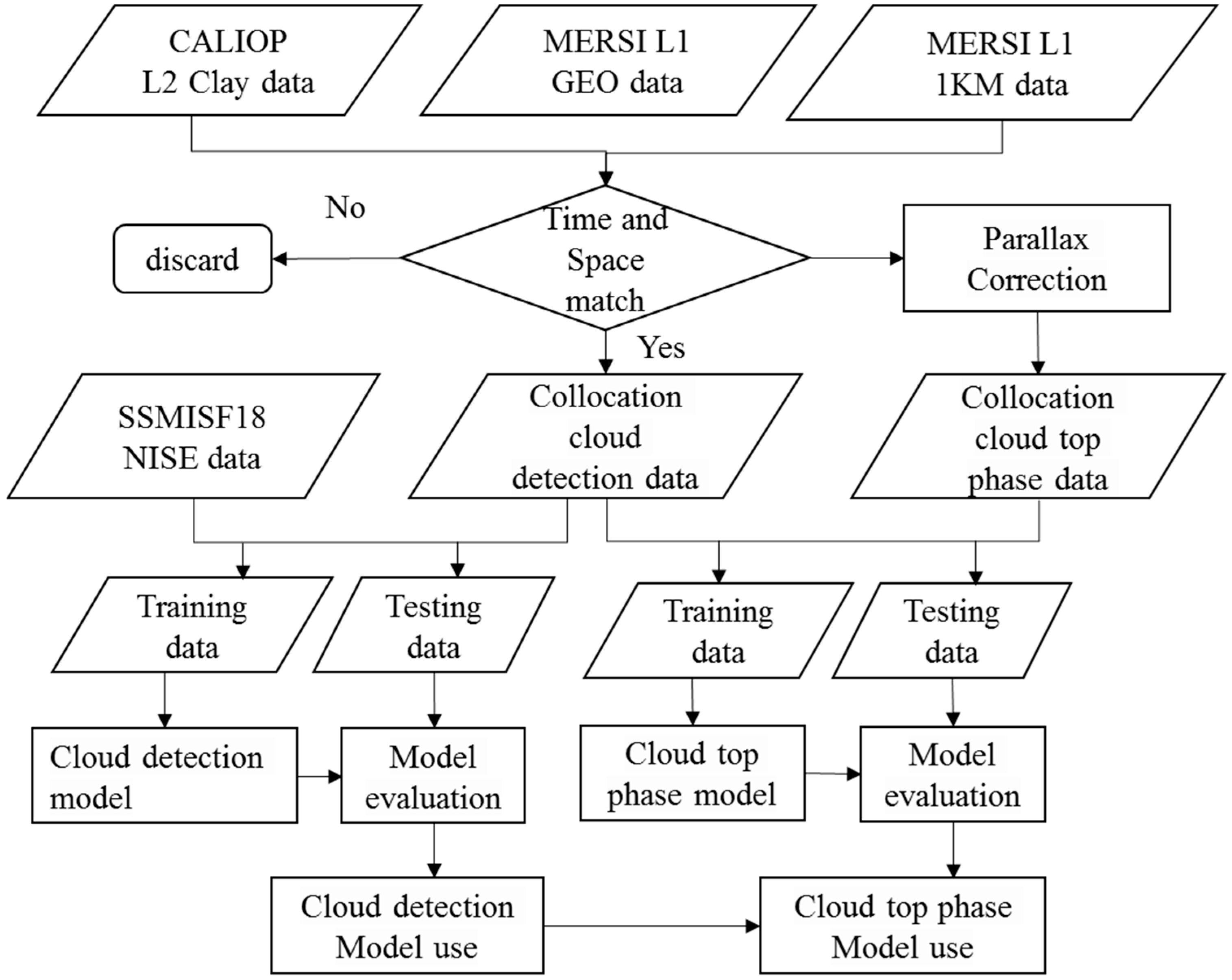
Figure 1 illustrates the flow of data processing and machine learning model building in this study. It involves spatial and temporal matching of CALIOP and MERSI-II sensors, followed by parallax correction to establish collocated datasets. The collocated datasets retain only data with reliable cloud detection and cloud-top thermodynamic phase identification results. The collocated datasets provide input values and true labels for the cloud detection and cloud-top thermodynamic phase model. The infrared channel data from the 1 km product of the MERSI-II sensor, as well as the Arctic ancillary information provided by the L1_GEO data of the MERSI-II sensor, are used as inputs for the models. The CALIOP cloud detection and cloud-top thermodynamic phase identification values serve as the true labels for machine learning models. AdaBoost (Adaptive Boosting) machine learning method is then employed to establish and optimize cloud detection and cloud-top thermodynamic phase models for different surface types in the Arctic region. In the process of model application, we first utilize the established model for cloud detection. Based on the cloud detection results, for the cloudy areas, we then employ the cloud-top thermodynamic phase model to discriminate the cloud-top thermodynamic phase.

To enhance the generalization ability of the models and ensure their reproducibility, 70% of the matched dataset is randomly selected as the training sample, while the remaining 30% is used as the test sample. A training dataset of 626,000 pixels and a test dataset of approximately 268,200 pixels are used in the paper. The inversion performance of the models was then rigorously evaluated using a completely independent dataset collected in July 2022.

2.1. CALIOP and MERSI-II Data

CALIOP can accurately obtain cloud information in the atmosphere, with a mature cloud phase identification product, which is widely used in the validation and evaluation of cloud products from passive satellite remote sensing instruments [39,40,41,42]. The CALIOP sensor uses 532 nm and 1064 nm lasers to measure aerosols and cloud layers in the atmosphere. The polarization signal at 532 nm is often used in cloud phase identification algorithms due to its strong dependence on particle shape [43]. In this study, we used the CALIOP Level2 1 km cloud layer product (CAL_LID_L2_01kmCLay-Standard-V4-20), which classifies cloud layers into water clouds, randomly oriented ice clouds, or horizontally oriented ice clouds based on the relationship between depolarization ratio, backscatter intensity, temperature, and attenuated backscatter color ratio. In cases where the identification is unclear, the phase is defined as “unknown/undetermined”. The algorithm discards cloud layers with multiple phases present. The study only selects data from the CALIOP product that are identified as water clouds and ice clouds. Based on the identification of the ice-water phase quality flag, the identification result is required to reach a trust level of medium or higher, i.e., Ice/Water Phase QA ≥ 2. The selected CALIOP cloud phase data serves as the true value of cloud phase provided during the model training and validation stages.

The CloudSat satellite is furnished with a 94 GHz Cloud Profiling Radar (CPR) sensor, which is extensively employed for examining global cloud profiles and their spatiotemporal variations. Nevertheless, the CPR’s frequency has a propensity for greater sensitivity to optically thick clouds, rendering it unable to discern optically thin clouds. Conversely, CALIOP exhibits a high degree of sensitivity to minute particles located at the cloud top. Consequently, in this research endeavor, CALIOP data alone is adopted as the gold standard for cloud detection and determination of cloud phase.

The FY-3 meteorological satellite is China’s second-generation polar-orbiting meteorological satellite, aiming to achieve all-weather, multi-spectral, and three-dimensional observations of global atmospheric and geophysical elements, providing meteorological parameters for medium-range numerical weather forecasting and monitoring large-scale natural disasters and ecological environments. The Medium Resolution Spectral Imager-II (MERSI-II) carried by the FY3D satellite is equipped with a total of 25 channels, including 16 visible-near-infrared channels, 3 shortwave infrared channels, and 6 medium-longwave infrared channels. For specific band information and detailed introductions, please refer to the official website at http://www.nsmc.org.cn/nsmc/cn/instrument/MERSI-2.html, accessed on 28 August 2025.

In this study, the brightness temperature data from the infrared channels (channels are abbreviated as CH) of the MERSI-II sensor’s L1_1km product were primarily used as input for research on an all-weather Arctic cloud detection model. The relevant channels and performance parameters can be obtained from the following link: http://space-weather.org.cn/nsmc/cn/instrument/MERSI-2.html, accessed on 28 August 2025. Among them, CH20 and CH21 are located in the mid-wave infrared region, where there is not only emitted radiation but also reflected radiation information during the daytime. CH22 is located in the water vapor absorption region, CH24 is an atmospheric window channel, and CH25 is an atmospheric split-window channel with minor water vapor absorption. The L1_GEO data of MERSI-II stores geographically located spherical observation data after preprocessing. In this study, 5 min and 1 km spatiotemporal resolution GEO data were used for spatiotemporal matching with the CALIOP cloud product.

2.2. Ancillary Data

The GEO files provided by the MERSI-II include Land Cover products, which define 17 land cover types according to the International Geosphere-Biosphere Programme (IGBP). These include 11 natural vegetation types, 3 land development and mosaic land types, and 3 non-vegetated land type definitions. The product codes and classifications are as follows: 0—water, 1—evergreen needleleaf forest, 2—evergreen broadleaf forest, 3—deciduous needleleaf forest, 4—deciduous broadleaf forest, 5—mixed forest, 6—dense shrubland, 7—open shrubland, 8—woody savanna, 9—savanna, 10—grassland, 11—permanent wetlands, 12—croplands, 13—urban and built-up areas, 14—cropland/natural vegetation mosaic, 15—snow and ice, 16—bare ground.

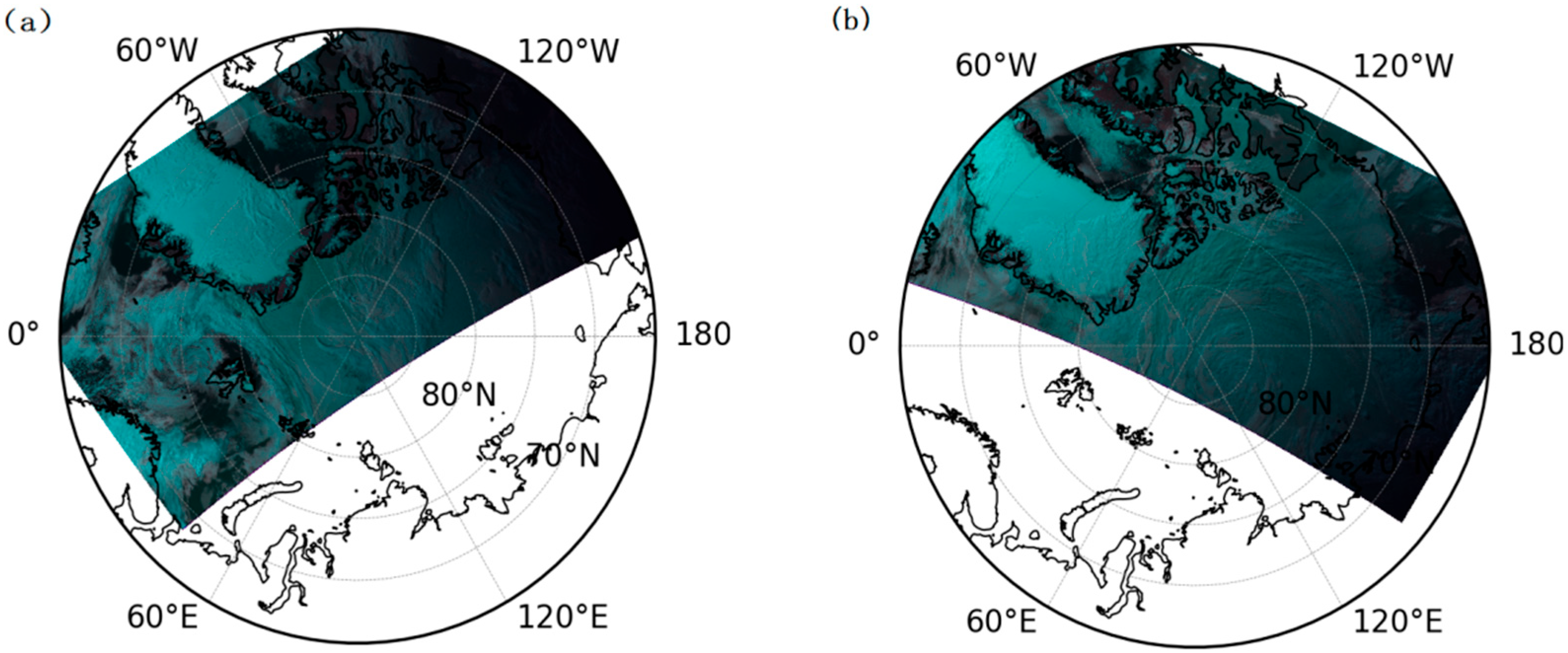
In the study, the AdaBoost model was trained for different surface types. The Arctic region has extremely low temperatures, often below minus tens of degrees Celsius, with most areas covered by glaciers and the surface soil layer permanently frozen. Figure 2 shows the Arctic surface types generated based on the Land Cover product in July 2021, revealing that the Arctic mainly includes five surface types: water bodies, evergreen needleleaf forests, open shrubland, grasslands, and ice and snow. Additionally, there are extremely small amounts of permanent wetlands, urban and built-up areas in the Arctic, but they occupy a very small proportion of the total area. Based on the Arctic surface classification, this study established cloud detection and cloud phase identification models for the aforementioned five surface types, respectively.

Due to the small temperature difference between clouds and ice/snow, the radiative difference between clouds and the ice/snow underlying surface is also small, making cloud detection very challenging. Therefore, this study uses sea ice as an auxiliary input to the model to reduce modeling errors. The fifth version of daily global sea ice concentration and snow cover data (NISE_SSMISF18_YYYYMMDD.HDF-EOS) from the National Snow and Ice Data Center (NSIDC) in the United States, which are based on the Special Sensor Microwave Imager (SSM/I), is utilized as auxiliary data for surface type classification. The data can be obtained from the website: https://nsidc.org/data/nise/versions/5, accessed on 28 October 2024. This data is stored in HDFEOS format, with the Extent dataset recording the sea ice concentration for each pixel and including markers for permanently glaciated areas. Based on the Extent data, pixels with sea ice coverage are recorded as 1, and pixels without sea ice are recorded as 0, serving as input data for the prediction model.

2.3. Spatiotemporal Matching

Select the high-latitude region north of 65°N as the study area, and use the 2021 FY3D/MERSI-II data and CALIOP Level2 cloud layer product data for spatiotemporal matching. The matching algorithm is as follows: Based on the overpass time of the CALIOP sub-satellite point, select the FY3D satellite orbits that pass over within 5 min before and after it. Using the CALIOP sub-satellite point as the center, calculate the distance between all MERSI-II pixels and the CALIOP sub-satellite point using the Haversine formula. If the distance between the pixel and the CALIOP sub-satellite point does not exceed 1 km, it is considered a matched pixel.

$$\mathrm{d}=2\mathrm{R}\times \mathrm{a}\mathrm{r}\mathrm{c}\mathrm{s}\mathrm{i}\mathrm{n}\sqrt{{\mathrm{s}\mathrm{i}\mathrm{n}}^2\left({\displaystyle \frac{{\mathrm{l}\mathrm{a}\mathrm{t}}_2-{\mathrm{l}\mathrm{a}\mathrm{t}}_1}{2}}\right)+\cos \left({\mathrm{l}\mathrm{a}\mathrm{t}}_1\right)\times \mathrm{c}\mathrm{o}\mathrm{s}({\mathrm{l}\mathrm{a}\mathrm{t}}_2)\times {\mathrm{s}\mathrm{i}\mathrm{n}}^2({\displaystyle \frac{{\mathrm{l}\mathrm{o}\mathrm{n}}_2-{\mathrm{l}\mathrm{o}\mathrm{n}}_1}{2}})}$$

(1)

where d is the distance between the two points, R is the radius of the Earth (approximately 6371 km), lat₁ and lat₂ are the latitude coordinates of the two points, and lon₁ and lon₂ are the longitude coordinates of the two points. Both latitude and longitude coordinates need to be expressed in radians. The Haversine formula eliminates the influence of cosine calculations and does not have excessively high requirements for the precision of floating-point operations in the system during short-distance calculations.

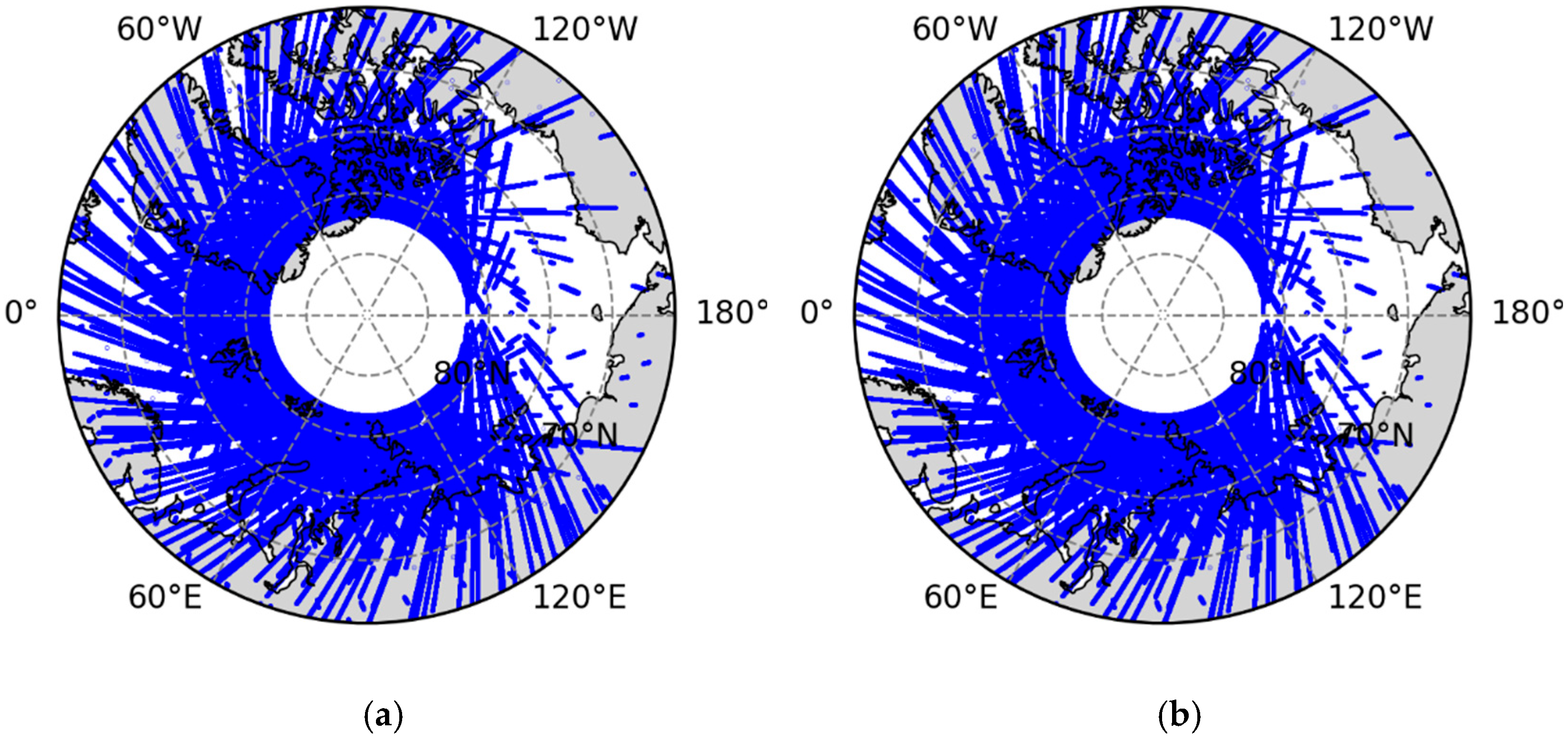
Precise spatiotemporal matching can minimize uncertainties arising from spatial and temporal sampling differences. For the MERSI-II sensor, in the case of a large view zenith angle (VZA), the area of the ground pixel will correspondingly increase. After performing the aforementioned spatiotemporal matching, pixels with VZA exceeding 45° in MERSI-II are further discarded. Figure 3 shows the distribution of CALIOP orbits matched with MERSI-II in the Arctic region for 2021.

2.4. Parallax Correction

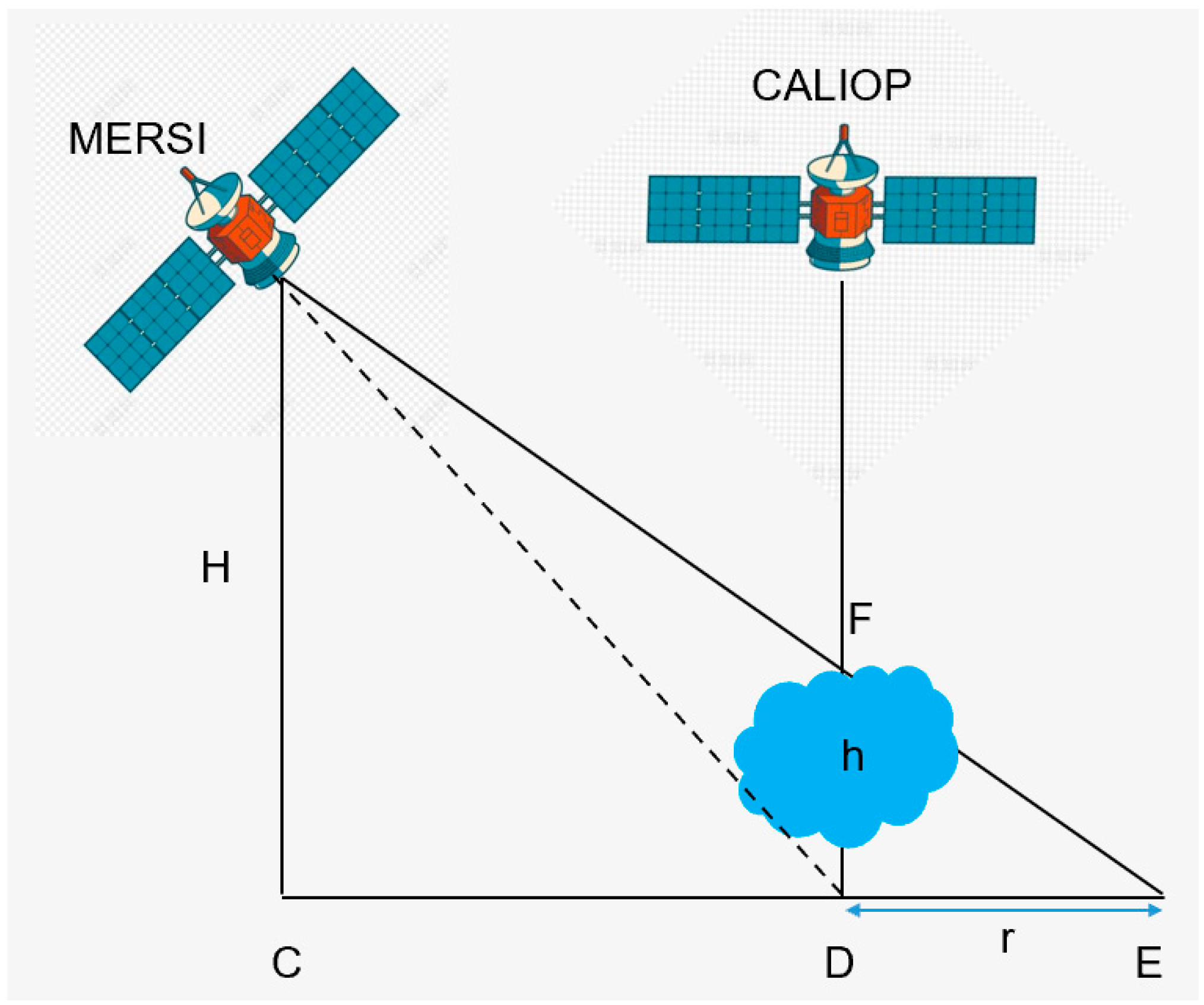
CALIOP is a vertically downward-looking instrument, while MERSI-II is an oblique-viewing instrument (Figure 4). If matching is based on the ground footprint (point D in the figure), the cloud information observed by MERSI-II is not from the sub-satellite point of CALIOP, but rather from the cloud information along the dashed line path, ultimately introducing erroneous information. To obtain correct matching results, the measurement value at point E, which is the ground footprint detected by MERSI-II, should be used.

Therefore, it is necessary to further perform parallax correction on the matched pixels of MERSI-II and CALIOP, using the method described by Wang et al. [44]. The displacement vector $\overrightarrow{|\mathrm{r}}|$ is represented as follows:

$$\overrightarrow{|\mathrm{r}}|=\mathrm{hHtan}\theta /(\mathrm{H}-\mathrm{h})$$

(2)

where H is the operational altitude of MERSI-II, h is the cloud-top height identified by CALIOP, and θ is the viewing zenith angle of MERSI-II at point D.

The viewing azimuth angle (the angle between CD and the geographic north) is denoted as ϕ, and the latitude and longitude of point D are represented in radians as Y_D and X_D, respectively. Then, the displacement vector can be projected onto latitude and longitude to uniquely determine the coordinates of point E. All angles and coordinates are in radians, and R_E is the radius of the Earth (approximately 6371 km). We used the following equations to quantitatively calculate the latitude and longitude of point E:

$${\mathrm{Y}}_{\mathrm{E}}={\mathrm{Y}}_{\mathrm{D}}+\overrightarrow{|\mathrm{r}}|\cos \varnothing /{\mathrm{R}}_{\mathrm{E}}$$

(3)

$${\mathrm{X}}_{\mathrm{E}}={\mathrm{X}}_{\mathrm{D}}+\overrightarrow{|\mathrm{r}}|\sin \varnothing /({\mathrm{R}}_{\mathrm{E}}\cos {\mathrm{Y}}_{\mathrm{D}})$$

(4)

3. Model Configuration and Training

3.1. AdaBoost Model and Evaluation Metrics

The AdaBoost algorithm was first proposed by Freund and Schapire in 1997. In classification problems, it improves classification performance by adjusting the weights of training samples to learn multiple classifiers, which are then linearly combined to integrate multiple weak classifiers into a strong classifier. The AdaBoost process can be divided into the following steps: initializing the weights of the training set and training a base learner from the initial set; increasing the weights of misclassified samples and decreasing the weights of correctly classified samples; increasing the weights of base learners with lower error rates and decreasing the weights of those with higher error rates; training the next base learner using the adjusted (and normalized) sample weights; repeating the process until the specified number of base learners is reached; and finally, combining these base learners with weights to perform voting.

Using the CALIOP cloud products as a reference, we define cloudy or ice cloud pixels as positive events, clear or water cloud pixels as negative events, respectively. The true positive rate (TPR) and false positive rate (FPR) were used to evaluate the prediction results of the deep learning model. We aim to build a model that is sensitive to both clear skies and cloudy conditions, capable of identifying the majority of clouds while also minimizing the misidentification of clear skies as cloudy. Therefore, high TPR and low FPR are required. The TPR and FPR are defined as follows:

$$\mathrm{T}\mathrm{P}\mathrm{R}={\displaystyle \frac{\mathrm{T}\mathrm{P}}{\mathrm{T}\mathrm{P}+\mathrm{F}\mathrm{N}}}$$

(5)

$$\mathrm{F}\mathrm{P}\mathrm{R}={\displaystyle \frac{\mathrm{F}\mathrm{P}}{\mathrm{F}\mathrm{P}+\mathrm{T}\mathrm{N}}}$$

(6)

TP and TN are the number of cloud and clear pixels that are correctly detected, whereas FP and FN are the number of pixels that are misidentified by the model (

Table 1. Confusion matrix of truth labels of samples and prediction results.

Confusion Matrix	Cloud Detection Model
	Cloud	Clear
Cloud (positive)	TP	FN
Clear (negative)	FP	TN

).

The paper employs the Accuracy and F1 Score to reflect the algorithm’s accuracy from multiple perspectives. Accuracy signifies the ratio of correctly classified samples to the overall count of samples. F1 Score is the harmonic mean of precision and recall. A higher F1 score indicates better overall performance. The equations are as follows:

$$\mathrm{A}\mathrm{c}\mathrm{c}\mathrm{u}\mathrm{r}\mathrm{a}\mathrm{c}\mathrm{y}={\displaystyle \frac{\mathrm{T}\mathrm{P}+\mathrm{T}\mathrm{N}}{\mathrm{T}\mathrm{P}+\mathrm{F}\mathrm{N}+\mathrm{F}\mathrm{P}+\mathrm{T}\mathrm{N}}}$$

(7)

$$\mathrm{P}\mathrm{r}\mathrm{e}\mathrm{c}\mathrm{i}\mathrm{s}\mathrm{i}\mathrm{o}\mathrm{n}={\displaystyle \frac{\mathrm{T}\mathrm{P}}{\mathrm{T}\mathrm{P}+\mathrm{F}\mathrm{P}}}$$

(8)

$$\mathrm{F}1 \mathrm{s}\mathrm{c}\mathrm{o}\mathrm{r}\mathrm{e}=2{\displaystyle \frac{\mathrm{P}\mathrm{r}\mathrm{e}\mathrm{c}\mathrm{i}\mathrm{s}\mathrm{i}\mathrm{o}\mathrm{n}\times \mathrm{T}\mathrm{P}\mathrm{R}}{\mathrm{P}\mathrm{r}\mathrm{e}\mathrm{c}\mathrm{i}\mathrm{s}\mathrm{i}\mathrm{o}\mathrm{n}+\mathrm{T}\mathrm{P}\mathrm{R}}}$$

(9)

3.2. Model Configuration

When using the AdaBoost model, appropriately selecting and tuning hyperparameters can enhance the model’s performance, allowing it to better adapt to various datasets and tasks. The performance of the AdaBoost model is jointly determined by its inputs (channels or other information) and parameter configurations (such as n_estimators and max_depth).

The radiative differences between clouds and snow/ice surfaces are relatively small, which makes it easy for optical sensors to produce errors in distinguishing between clouds and snow/ice. Therefore, based on the research results of Wang et al. [28] and in combination with the infrared band channel settings of FY3D/MERSI-II, the brightness temperature of window channels and the brightness temperature differences are selected as model inputs. These include the brightness temperature differences between CH20 and CH25, CH24 and CH20, CH23 and CH24, CH20 and CH21, as well as the brightness temperatures of CH22 and CH24. Additionally, the model inputs also include parameters such as VZA, longitude (lon), latitude (lat), solar zenith angle (SZA), and sea ice density (ICE).

Clouds and clear-sky underlying surfaces exhibit distinct emission radiation characteristics in infrared wavelengths. Numerous studies have demonstrated that brightness temperature differences across different infrared channels can be effectively utilized not only for cloud classification but also for distinguishing clouds from underlying snow/ice surfaces. Snow and ice surfaces demonstrate strong specular reflection properties, with their reflectance increasing sharply as the satellite VZA increases. This characteristic leads to radiation signal confusion between ice/snow and clouds during observations at large VZAs. Incorporating VZA into the model can correct geometric observational discrepancies and enhance consistency in radiometric signatures. The surface temperature and radiometric properties of the Arctic exhibit nonlinear variations with latitude, lon, and lat provide critical prior information that accelerates model convergence. The introduction of SZA enables effective mitigation of atmospheric scattering interference. ICE directly influences surface emissivity in the 10.8 μm and 12.0 μm channels; therefore, incorporating ICE into the model allows for quantitative characterization of surface coverage states and reduces confusion between ice/snow and clouds.

In terms of parameter configuration, n_estimators represents the number of weak learners to be constructed in the algorithm, and max_depth characterizes the maximum depth of the decision trees. When parameter values are excessively high, the model risks overfitting; conversely, when they are too low, the model may suffer from underfitting. Through testing of model configurations, the accuracy scores for these surface types are less sensitive to these model parameters when using more than 100 weak classifiers and a maximum tree depth of 10. Therefore, we use the configuration n_estimators = 100 and max_depth = 10 to train the model.

To evaluate the overall performance of the model, we defined an accuracy rate. In the study, accuracy refers to the proportion of samples where the cloud and clear-sky identification results based on the AdaBoost model agree with CALIOP, relative to the total number of samples. By comparing the model’s performance under different input variables and parameter configurations, we ultimately selected a model that exhibits relatively high accuracy while also saving computational time.

Table 2. Accuracy scores of AdaBoost cloud detection models based on testing pixels.

No.	Model Input	Water	Shrubland	Snow and Ice	Barren	Forest	Grasslands	All
1	B20_25, B24_20, B23_24, B20_21, B22, B24, lon, lat	0.898	0.898	0.910	0.880	0.913	0.859	0.892
2	B20_25, B24_20, B23_24, B20_21, B22, B24, lon, lat, VZA	0.897	0.900	0.906	0.890	0.932	0.862	0.904
3	B20_25, B24_20, B23_24, B20_21, B22, B24, lon, lat, VZA, SZA	0.900	0.896	0.908	0.882	0.931	0.863	0.910
4	B20_25, B24_20, B23_24, B20_21, B22, B24, lon, lat, VZA, SZA, ICE	0.898	0.904	0.904	0.882	0.923	0.857	0.911
5	B20_25, B24_20, B23_24, B20_21, B22, B24, lon, lat, VZA, ICE	0.898	0.893	0.909	0.888	0.911	0.851	0.905

presents the training and testing accuracy scores for the cloud detection model based on infrared channels under different inputs. It indicates that the model achieves the best overall accuracy scores across all surface types under the model input conditions numbered 3 and 4. Considering the costs of data acquisition and model computation comprehensively, we ultimately chose model 3.

4. Results

4.1. Evaluation of AdaBoost Model Results

TPR and FPR are two critical parameters in model evaluation. A perfect model should have a high TPR and a low FPR, with TPR ideally approaching 1 and FPR ideally approaching 0 [45].

Figure 5a illustrates the distribution of TPR and FPR for various surface cloud detection models. The TPR, which indicates the correct identification of clouds, averages at 91.9% across all surface models, while the FPR, representing false positives, stands at 12.0%. These models exhibit relative stability in performance across diverse surface types, with slight variations for each specific surface category. Notably, the model tailored for snow and ice surfaces (denoted by green circles) demonstrates the superior performance, achieving a TPR of 94.2% and an FPR of 8.9%. Models designed for water, shrubland, forest, and barren exhibit comparable performance metrics.

Furthermore, Figure 5b presents the TPR and FPR for cloud-top thermodynamic phase models. Across all surface models, the overall TPR (correct identification of ice clouds) for correctly identifying ice clouds is 94.6%, accompanied by an FPR of 9.4%. Notably, the model for grasslands exhibits a slightly inferior performance compared to the other surface models, with a TPR of 89.0% and an FPR of 10.3%. Conversely, the performance of the other models is more favorable.

Table 3. The evaluation results of cloud detection and cloud-top thermodynamic phase identification models on different land surfaces.

Surface Types	Cloud Detection		Cloud-Top Thermodynamic Phase
	Accuracy	F1 Score	Accuracy	F1 Score
Water	0.904	0.881	0.931	0.927
Shrubland	0.910	0.899	0.940	0.940
Snow and Ice	0.925	0.925	0.942	0.940
Barren	0.896	0.889	0.934	0.934
Grasslands	0.881	0.867	0.893	0.892
Broadleaf Forest	0.932	0.922	0.911	0.911
All	0.916	0.901	0.928	0.927

provides the accuracy and F1 scores for cloud detection models across various surface types. The overall model achieves an F1 score of 0.9. Among the models evaluated, the snow and ice surface model shows the highest performance, with all scores exceeding 0.92. In contrast, the grassland model demonstrates a lower performance compared to the other models, with an F1 score of 0.87. Regarding cloud-top thermodynamic phase models, the overall F1 score for all samples is 0.93. Among the surface-specific models, the snow and ice surface model performs best, with all scores surpassing 0.94. Similarly, the grassland model demonstrates lower accuracy and F1 score than the other models, with an F1 score of 0.892 and an accuracy of 0.893.

4.2. Verification and Analysis of Cloud Detection Model

To comprehensively assess the cloud detection model and cloud-top thermodynamic phase identification developed in this study, we selected MERSI-II observation scenes from diverse regions and underlying surfaces within the Arctic in July 2022. These scenes were analyzed in conjunction with MERSI-II false color images and cloud detection/cloud-top thermodynamic phase products from various satellites. The results were presented, and the model’s performance was thoroughly analyzed and discussed.

Figure 6a is the infrared brightness false color image of MERSI-II at 11:35 on 16 July 2022. This image, synthesized using channels at 0.685, 0.865, and 1.65 μm, provides an intuitive representation of cloud distribution. Figure 6c presents the MERSI-II cloud detection product (shaded) alongside the cloud detection results (line) along the CALIOP track, which passed within the same timeframe (<5 min). The CALIOP cloud detection product utilizes red dots to signify cloud labels and yellow dots for clear labels. Within area A, enclosed by the pink square, the underlying surface comprises snow and ice, barren land, and water. The false color image reveals that most of the area is clear-sky, and the CALIOP cloud detection product accurately identifies this. While MERSI-II identifies some clear-sky areas, these are significantly smaller compared to the false color image, suggesting over-detection of clouds. In contrast, the AdaBoost model, as shown in Figure 6e, effectively identifies the clear-sky view within the pink square. Similarly, the false color image of area B, also enclosed by the pink square, indicates that most of the area is clear-sky. MERSI-II identifies most of this area as possibly clear or undetermined, whereas the AdaBoost model successfully identifies the clear sky.

Figure 6b presents a false-color image captured at 15:25 on 9 July 2022. The area within the pink square depicts a clear-sky view over the snow-covered surface of the Greenland continent. The CALIOP cloud detection product accurately identifies clear skies in this region, whereas the MERSI-II cloud detection product is unable to make a determination. Figure 6f displays the cloud detection result of the AdaBoost model, which effectively identifies the clear-sky view within the pink square. The overall distribution of clear sky and clouds obtained by the AdaBoost model aligns well with the distribution shown in the false-color image.

4.3. Verification and Analysis of Cloud-Top Thermodynamic Phase Model

The cloud-top thermodynamic phase identification model developed in this study was subject to further evaluation, as shown in Figure 7. Similarly, Figure 7a,b depict infrared brightness false-color images obtained from MERSI-II, which are utilized to illustrate the actual distribution of clouds on the specified day. Figure 7c shows that at the CALIOP overpass trajectory at 13:15 on 16 July 2022. In area A, CALIOP identified the cloud-top thermodynamic phase as water clouds, whereas the MERSI-II cloud-top thermodynamic phase product labeled most of the area as uncertain. Figure 7e demonstrates that the AdaBoost cloud-top thermodynamic phase model constructed in this study can accurately identify water cloud regions. Specifically, for the clouds in area B (depicted in Figure 7c), CALIOP identifies them as ice clouds (indicated by red dots), whereas MERSI-II misidentified them as water clouds (cyan). However, our AdaBoost cloud-top thermodynamic phase model accurately identified the water clouds in area B (Figure 7e).

At 15:25 on 9 July 2022, along the CALIOP overpass track (Figure 7d), CALIOP identified area A as consisting of water clouds (yellow dots) and clear sky (gray dots). In contrast, the MERSI-II cloud-top thermodynamic phase product misidentified water clouds as ice clouds. The AdaBoost cloud-top thermodynamic phase model, however, was able to accurately identify both water clouds and clear sky areas. Regarding area B at the same time point, CALIOP identified ice cloud areas (red dots), which were mislabeled as water clouds by the MERSI-II cloud-top thermodynamic phase product (marked as the cyan-colored area). In contrast, the AdaBoost cloud-top thermodynamic phase model accurately identified the ice clouds (marked as the red-colored area) in Figure 7f.

5. Discussion

Our findings align favorably with recent advancements in machine learning-based Arctic cloud detection. For instance, the multi-information fusion cloud detection network utilizing POLDER-3 data reported 95.53% consistency with MODIS over ocean and ice-snow surfaces [35], while our approach maintains comparable accuracy using only infrared spectra. Unlike methods relying on multi-angle or polarization information, our model demonstrates that effective cloud detection and phase classification can be achieved with minimal input channels, potentially reducing computational complexity and data requirements.

However, this study still has some limitations: (1) While CALIOP provides excellent vertical resolution for cloud detection, its narrow swath creates spatial sampling limitations that inevitably affect training data comprehensiveness. In the dataset obtained through spatiotemporal matching, there is a relative scarcity of sample data within the 120°E–120°W range, and the uneven spatial distribution of training samples impacts the model’s performance. (2) In this study, VZA of the training samples was less than 40 degrees, resulting in increased uncertainty for cloud detection and identification of cloud-top thermodynamic phases at larger VZA. (3) Our approach exhibits sensitivity to surface emissivity variations—a particularly relevant concern in the Arctic, where snow and ice surface properties change rapidly with meteorological conditions. The reliance on infrared data alone makes our algorithm susceptible to errors when surface emissivity characteristics resemble those of clouds, especially under temperature inversion conditions common in polar regions. (4) Machine learning models focus on numerous parameters, and varying these parameter configurations can lead to diverse prediction outcomes. Future studies may concentrate on enhancing the precision of these models.

6. Conclusions

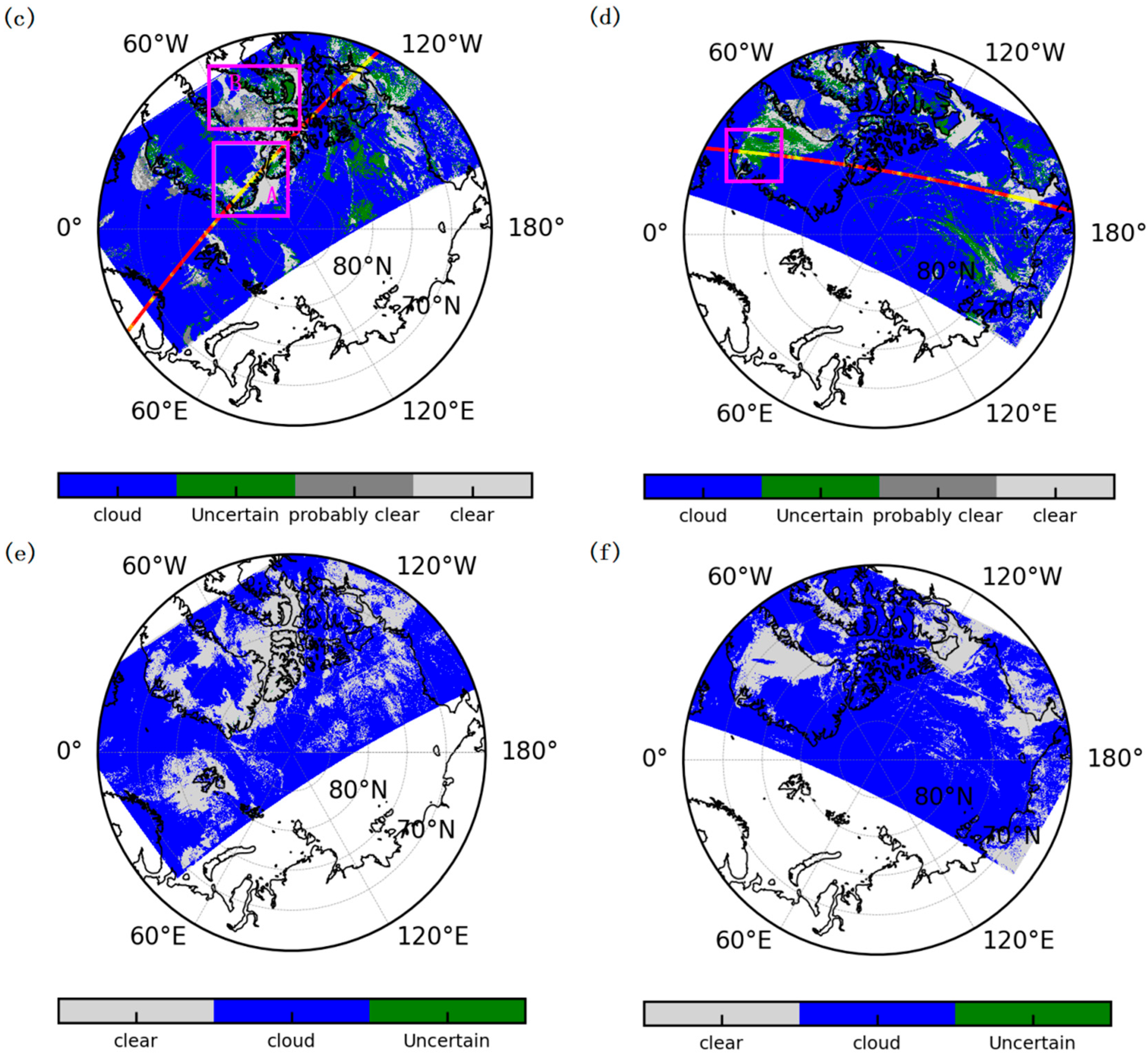
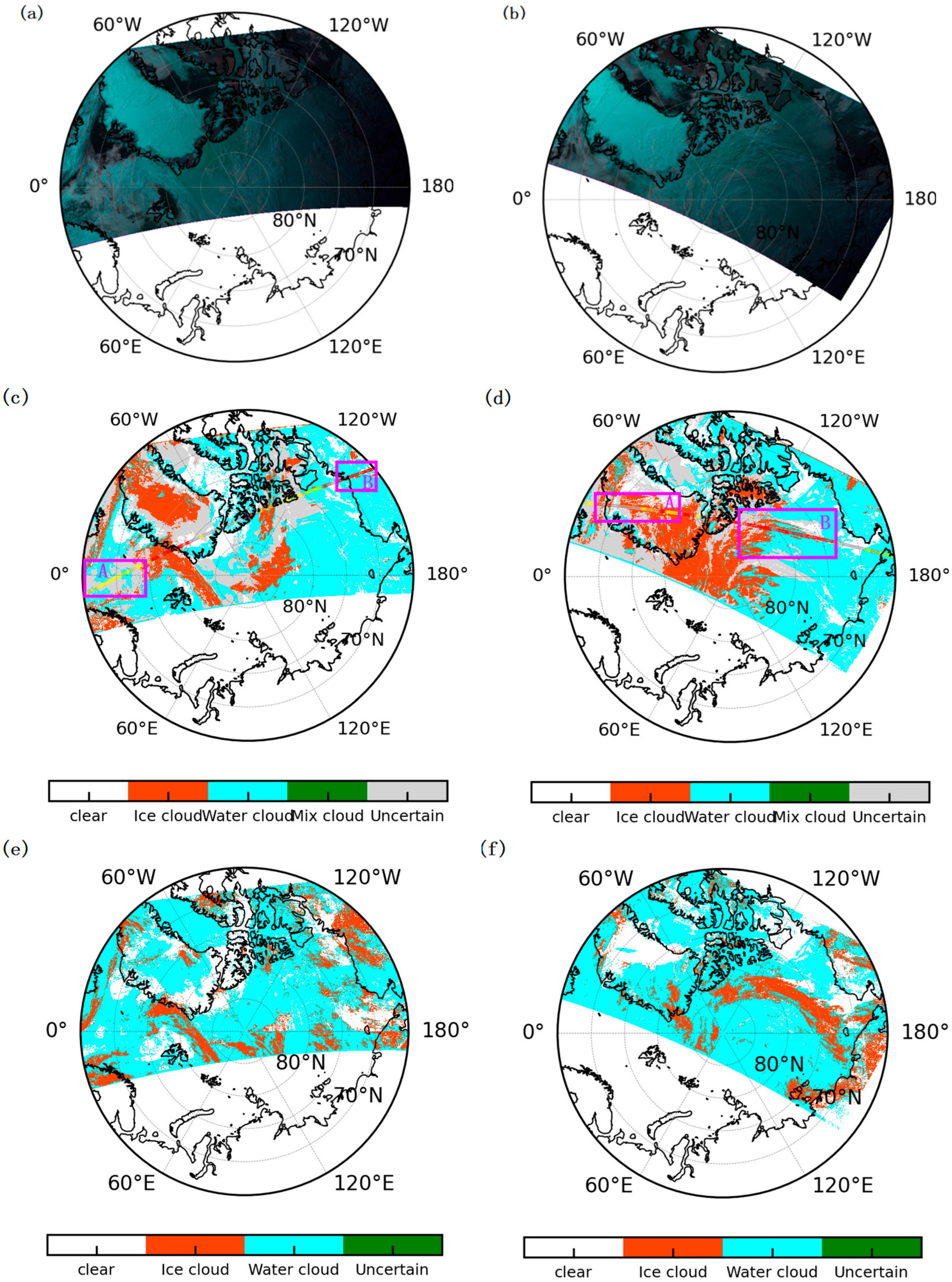
The performance of machine learning models is highly reliant on the quality of training samples and reference labels. CALIOP offers high reliability in cloud detection and cloud-top thermodynamic phase identification, thereby serving as a valid reference truth. In this paper, a spatiotemporal matched cloud parameter dataset was constructed using MERSI-II data from the FY-3D satellite and CALIOP cloud detection and cloud-top thermodynamic phase products for the year 2021. Based on this dataset, an AdaBoost machine learning algorithm was employed to develop a model for cloud detection and cloud-top thermodynamic phase identification at a 1 km resolution in the Arctic. The accuracy assessment of the machine learning model revealed that the cloud detection and cloud-top thermodynamic phase identification models achieved overall accuracies exceeding 91.6% and 92.8%, respectively, in the Arctic. Examination of the validation dataset demonstrated that the cloud detection and cloud-top thermodynamic phase models had the ability to correctly recognize clear skies that were mistakenly labeled as clouds in MERSI-II data, as well as accurately differentiate between ice clouds and water clouds that were incorrectly identified. The results of the models exhibited high consistency with CALIOP products, and the clear sky-cloud and ice-water cloud distribution obtained by the models aligned well with the identification results derived from false-color images.

The work presented in this paper also demonstrates that: (1) By utilizing machine learning methods, cloud detection and cloud-top thermodynamic phase identification in the Arctic can be achieved using solely raw infrared detection data, effectively addressing the issue of cloud parameter retrieval errors caused by the absence of visible light data during polar nights when using traditional threshold methods. (2) The dataset of Arctic cloud parameters established in this study, which combines CALIOP and MERSI-II, provides high-quality data for machine learning training and validation.