Abstract
The stochastic model in Precise Point Positioning (PPP) defines the statistical properties of observations and the dynamic behavior of parameters. An inaccurate stochastic model can degrade positioning accuracy, ambiguity resolution, and other aspects of performance. However, due to the influence of multiple factors, the stochastic model in PPP cannot be precisely predetermined, necessitating the development of an Adaptive Stochastic Model (ASM) based on Variance Component Estimation (VCE). While the benefits of ASMs for PPP float solutions are well documented, their contributions to other performance aspects remain insufficiently explored. This paper presents a comprehensive assessment of an ASM’s impact on PPP. First, the implementation of an ASM using VCE is described in detail. Then, experimental results demonstrate that the ASM effectively captures observational conditions through the estimated variance component factors. It enhances both PPP float and fixed solutions when the predefined stochastic model is inadequate, improves cycle-slip detection by tightening the stochastic model (reducing the missed detection rate from 19% to 8%), and accelerates both direct reconvergence and re-initialization after data gaps, with reconvergence times improved by 18% and 55%, respectively.
1. Introduction
GNSS Precise Point Positioning (PPP) is a global high-precision positioning method [1]. The PPP model comprises a functional model and a stochastic model. The latter describes the statistical properties of observational noise and process noise, serving as a critical component for data processing in PPP. A well-defined stochastic model is essential for optimal parameter estimation, reliable precision metrics, and effective hypothesis testing. Conversely, an improper stochastic model can degrade positioning accuracy [2], impact the detection of mismodeling errors with Detection, Identification, Adaptation (DIA) [3,4,5,6,7], and even result in incorrect ambiguity resolution [8,9,10]. The properties of stochastic noise are influenced by numerous factors, such as hardware design, observational environment, and even the time of day, making it challenging to capture these variations using a predefined stochastic model. Compared to other high-precision GNSS positioning methods like Real-Time Kinematic (RTK), PPP faces more complex stochastic noise characteristics due to its lack of support from regional GNSS networks. Thus, a real-time adaptive stochastic model is vital for refining the PPP model.
The PPP model is typically solved using the Kalman filter (KF), and the Sage–Husa adaptive KF is a classic algorithm for real-time stochastic model adjustment. The Sage–Husa algorithm is based on the principle that the a priori variance of the innovation vector can be expressed as a combination of observational noise variance and process noise variance. If one is accurately known, the other can be derived from the estimated innovation vector [11,12]. This algorithm is used extensively for dynamic positioning and navigation, such as GNSS integrated with Inertial Measurement Units (IMUs) [13,14], dead reckoning [15], and celestial navigation systems [16]. However, the Sage–Husa algorithm has notable limitations: it cannot simultaneously estimate both observational noise and process noise variances, and it requires estimating a full variance matrix, which often has more entries than just the innovation vector and cannot be estimated stably.
Variance Component Estimation (VCE) is another well-established algorithm that uses redundant information to estimate the variance matrix. Unlike the Sage–Husa algorithm, VCE decomposes the variance matrix into a linear combination of predefined matrices and estimates their coefficients, termed variance factors. This approach avoids the challenges associated with estimating the full variance matrix and enables the simultaneous refinement of observational and process noise models. VCE has been extensively used in post-processing applications, such as refining stochastic models with inter-frequency and temporal correlations [17,18,19] and stochastic models for multi-frequency observations [19,20]. Recent studies have explored integrating VCE with the Kalman filter for real-time stochastic model refinement. Some of them focused on the enhancement of stochastic models, such as applying Helmert’s simplified VCE to GPS Standard Point Positioning (SPP) [21], refining the stochastic model of PPP with Online-VCE [22], and the joint estimation of the variances of the dual-frequency GNSS observational noise and the process noise of the receiver code bias [23]. These studies are valuable to the analysis of stochastic models but did not present the benefits to the performance of refined stochastic models. Regarding the benefits of VCE to the performance of GNSS data processing, several different topics have been covered. Regarding the positioning performance, Zhang et al. combined modified VCE and Helmert VCE to improve observation weighting for PPP [24], while Zhang and Zhao adjusted the unit weight variance factor of the pseudo-range and the carrier-phase observations [25]; these results showed improvements in positioning accuracy, stability, and convergence time. For the estimation of non-positioning parameters, Yang et al. developed an adaptive KF using VCE to adjust the process noise variance for tropospheric delay of PPP, significantly improving the root-mean-square (RMS) error of tropospheric delay estimates [26]. For the quality control of data processing, Chang et al. used VCE to refine the stochastic model for ionospheric process noise in a cycle-slip repair algorithm [27], and the results showed that all manually introduced nontrivial cycle slips were correctly repaired.
These studies highlight the benefits of an Adaptive Stochastic Model (ASM) in various aspects of GNSS applications, including improved observational stochastic modeling, enhanced positioning precision, and refined tropospheric delay estimates; meanwhile, many of them are based on a PPP model which retains parameters for systematic errors and needs precise modeling of these parameters [22,24,25,26]. However, many aspects of GNSS PPP that depend on a proper stochastic model remain underexplored. For instance, ambiguity resolution (AR) typically involves two steps: decorrelation using Z-transformation and ambiguity fixing [28,29]. The Z-transformation operates on the variance matrix of ambiguities [30] while the success rate of fixing is calculated using the variance matrix [31]. Similarly, mismodeling detection algorithms such as DIA rely on hypothesis testing, whose effectiveness is determined by the quality of the stochastic model [32]. Furthermore, when satellite signals are interrupted, a dynamic model with an appropriate process noise model can better link epochs before and after the interruption, accelerating reconvergence and improving performance after data gaps [33,34,35]. However, it is incomplete to study only the benefits of an ASM for applicational problems; the value of an ASM to PPP lies in reflecting observational conditions through refined stochastic modeling, which should be assessed first. For a better understanding of the value of the ASM algorithm to PPP, an ASM algorithm is designed based on VCE and its influences on several topics of PPP are analyzed, including reflecting observational conditions through the estimation of time-variant variance factors, PPP float solution, PPP-AR, cycle-slip detection with DIA, reconvergence after data interruption, and interruption repair. The remaining sections are as follows: Section 2 proposes the ASM algorithm for the Kalman filter and the mathematical model of PPP; Section 3 evaluates the benefits of ASM across various PPP applications; and Section 4 summarizes the conclusions.
2. Materials and Methods
2.1. ASM for the Kalman Filter
In this section, the ASM for the Kalman filter is proposed, which is implemented with VCE. There are many VCE methods, including the Minimum Norm Quadratic Unbiased Estimator (MINQUE) [36], the best invariant quadratic unbiased estimator (BIQUE) [37], and the Least-Squares-VCE (LS-VCE) [38,39]. The LS-VCE is based on the well-known least-squared principle, which is more versatile and will be used to construct our ASM method. The LS-VCE will be introduced first; then, the implementation of the LS-VCE for the Kalman filter model will be derived; finally, the implementation of the ASM for the Kalman filter will be provided.
2.1.1. LS-VCE
Assume a linear observational model as
where is the observational vector, is the design matrix, is the estimable parameter, is the observational noise, is the variance matrix of , is the known part of variance matrix, and is the variance factor with corresponding matrix . A normal equation for the estimation of can be formed as follows:
where is the estimated value of , and the entries of and are calculated with
For , where is the projector of the orthogonal complement of , and the column space of [40]; obtains the trace of a matrix. The estimated variance factor is and the variance of is .
2.1.2. LS-VCE for the Kalman Filter
The dynamic model and observational model of the Kalman filter read
where and are the system states at epoch and , respectively; is the state transition matrix; is the process noise with the corresponding variance matrix ; is the observational vector; is the design matrix; and is the measurement noise with the corresponding variance matrix . Assume the estimated system state at epoch as
Then, the predicted system state at epoch can be obtained from the time update Equations (8) and (9), while the estimated system state can be obtained from the measurement update Equations (10) and (11).
where is the innovation vector, is the Kalman gain matrix, and is the variance matrix of . holds all the redundant information of the measurement update and can be used for determining the variance components of and . Assume that is divided as
while is divided as
The expression of can be rewritten in the form of (1) as
where the symbols in (1) are , , , , , . Furthermore, since , is simplified as and Equations (3) and (4) are simplified accordingly as
Then and can be estimated with the LS-VCE. The normal equation of the th epoch is noted as
2.1.3. Implementation of ASM
In most articles about refining stochastic models with VCE, data of several minutes or even hours are used for the estimation of one set of variance factors. However, the estimation in Equation (17) uses single-epoch data, which could be unstable due to the lack of redundant information. Meanwhile, the subtraction in Equation (16) may yield negative results, leading to negative estimated values of variance factors. To compensate the instability of single-epoch VCE, the single-epoch normal equations can be accumulated as Equation (18), where and form the accumulated normal equation of epoch . and for epoch are obtained from the initial value and variance matrix as and . The solution of and is with variance matrix .
However, when the estimated variance factors are time-variant, which happens when the observational environment changes, the accumulated estimations of the variance factors cannot reflect the temporal variation of the factors. To preserve the temporal characteristics of the estimated factors, a fading process is carried out as Equation (19) for , the estimation of last epoch, and its corresponding variance matrix before updating with Equation (18), where is a variance matrix for fading. is diagonal and its th diagonal entry reads , where is the fading factor for the th variance factor and the th diagonal entry of .
Figure 1 shows the estimations of the variance factor for pseudo-range observation. The single-epoch solution is noisy; with the normal matrices accumulated, the solution becomes so flat that it does not preserve any temporal variations; finally, with the fading process, the solution is both time-varying and smooth.
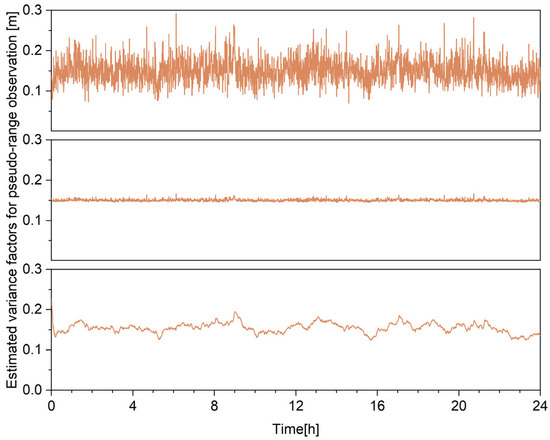
Figure 1.
The estimations of the variance factor for pseudo-range observation, single epoch (top), accumulating normal matrices of multiple epochs (middle), and with fading process (bottom).
The flow chart in Figure 2 shows the update of the Kalman filter with ASM. The update starts with system state and variance factor of the last epoch and observation of the current epoch; the green arrows show how the Kalman filter obtains the estimated system state of the current epoch, while the red ones show the process of updating the variance factor. Since the update of the variance factor is carried out after every update of the filter, it can be used for real-time applications.
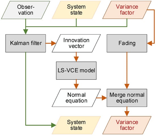
Figure 2.
Flow chart for the update of Kalman filter with ASM.
2.2. Data Processing Model of GNSS PPP
In this section, the multi-GNSS dual-frequency PPP model will be introduced. For the sake of simplicity, here we provide directly the full-rank observational equations. Equations (20) and (21) are the observational equations of pseudo-range and carrier-phase observations for GPS; Equations (22) and (23) are those of Galileo; and Equations (24) and (25) are those of BDS.
Superscript indicates the index of satellite, while subscripts and indicate the indices of frequency and epoch; and are pseudo-range and carrier-phase observations, respectively; is the approximated distance between satellite and receiver; is the positioning error with coefficient ; is the clock error of receiver; and are Inter-System Bias (ISB) for Galileo and BDS, respectively; is the zenith tropospheric wet delay with mapping function ; is the total electron content (TEC) in the unit of TECU, with that converts to signal delay on the th frequency band in meter; is the estimable ambiguity with wavelength ; and and are observational noise for pseudo-range and carrier-phase, respectively. Other systematic errors are corrected and omitted. , , , , , , and are set as parameters.
The dynamic model and observational model can be formed as Equations (5) and (6), where , , , for , for number of satellites; ; , ; , , for GPS, for Galileo, for BDS, with
Meanwhile, the variance matrices and are divided as
where is the elevational factor calculated with for the elevation of satellite ; is the ionosphere mapping factor; and are the positions of the satellite and receiver; is the position of the ionospheric piercing point of the single-layer ionospheric model, where is the unitary vector from receiver to satellite and is calculated by solving the equation ; and and are the length of the semi-major axis of Earth and height of the single-layer ionospheric model, respectively.
3. Results
In this section, the benefits of the ASM to several topics of PPP will be analyzed, including the estimation of variance factors, PPP float solution, PPP-AR, cycle-slip detection, reconvergence after data interruption, and interruption repair, where PPP tests are carried out for the model of Section 2.2 with either the predefined stochastic model or the ASM. Please note that although these tests are carried out in post-processing, the ASM can be used for real-time applications.
3.1. ASM Reflecting the Observational Conditions
To assess the ability of the ASM of reflecting the observational conditions, PPP tests with the ASM will be carried out for the model in Section 2.2 for global stations to obtain the estimated variance factors. Multi-GNSS observational data from 106 global stations on DOY 1~3 of 2023 is collected and processed with the configuration in Table 1. The precise products come from the Center for Orbit Determination in Europe (CODE), an analysis center of International GNSS Service (IGS), and include orbit, clock error, code bias, and phase bias [41,42].

Table 1.
Processing scheme for the analyses of variance factors.
3.1.1. Observational Noises of Pseudo-Range and Carrier-Phase Observations
Figure 3 shows the estimated variance factors of the pseudo-range observations for all stations, which are transformed to the unit of meter. The factors of the three systems vary around 0.1 m for most stations with visible temporal variations, which shows that the observational conditions are overall stable with slight fluctuations through time.
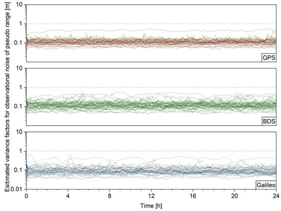
Figure 3.
Estimated variance factors of the pseudo-range observations for all stations.
Furtherly, Figure 4 shows the estimated variance factors of the carrier-phase observations for all stations. The curves of most stations vary around 1 mm for all three systems and the temporal variations are also preserved.
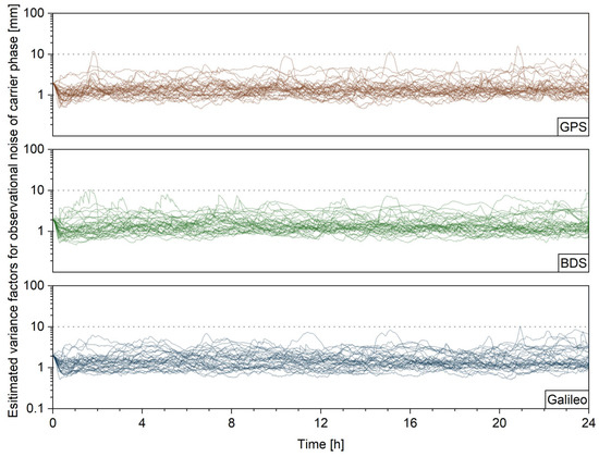
Figure 4.
Estimated variance factors of the carrier-phase observations for all stations.
Overall, the ASM can estimate the variance factors of both pseudo-range and carrier-phase observations and the temporal variations are preserved. It should be noted that the estimated factors are influenced by not only the observational noise but also systematic errors such as the precision of orbit/clock products. The factors reflect the overall observational conditions, which are influenced by multiple error sources; therefore, they can enhance the performance of positioning.
3.1.2. Process Noises of Atmospheric Parameters
Besides refining the observational stochastic model, the stochastic model of process noise is also improvable with an ASM. Figure 5 shows the estimated variance factors of ionospheric delay for all stations, where the x-axis is local time. The curves are correlated with local time and reach peak value at 12–18 every day, which matches the fact that the ionosphere is more active in daytime. It shows that the ASM is very helpful in adjusting the variance factor of ionospheric delay and could enhance cycle-slip detection, which requires refined ionospheric modeling for effective detection [43,44]. The enhancement of the ASM of cycle-slip detection with DIA will be examined in Section 3.4.
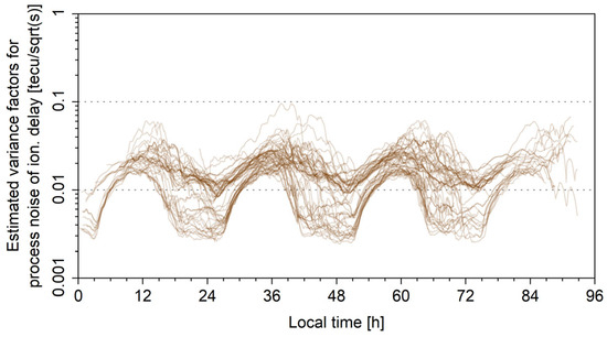
Figure 5.
Estimated variance factors of ionospheric delay for all stations.
Furtherly, Figure 6 shows the estimated variance factors of zenith tropospheric delay. The curves are almost straight lines, which shows that the factor of tropospheric delay is not estimable with the ASM and keeps its initial value. This is due to the fact that the variations of tropospheric delay between epochs are so small that they are overwhelmed by observational noises which are at least 10 times larger than them. However, the estimated factors do not diverge either, which shows that the algorithm is stable.
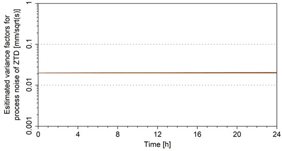
Figure 6.
Estimated variance factors of zenith tropospheric delay for all stations.
3.1.3. Process Noises of ISBs
Finally, Figure 7 shows the estimated variance factors of ISB. Like the factors of tropospheric delay, the curves are almost straight lines, which shows that the factors of ISB are not estimable with the ASM. This is due to the fact that the ISBs are linear combinations of receiver code biases, which are mostly stable.
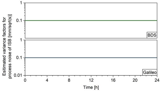
Figure 7.
Estimated variance factors of ISB for all stations.
3.2. Standard PPP Tests
In this section, PPP tests are carried out with an ASM (Adaptive) and without an ASM (Original) to show whether the positioning performance is improved with the proposed model.
3.2.1. PPP Results for Global Stations
Figure 8 shows the PPP positioning errors for IGS stations CHPG, MET3, and YAR3. The plots on the left and the right panels are very similar, which shows that the ASM has little impact on the performance.
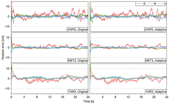
Figure 8.
PPP positioning errors without (left) and with (right) ASM.
Furtherly, with the solutions of global stations, the percentage of converged stations for different thresholds are shown in Figure 9 and the hists for 3D positioning errors are given in Figure 10. It shows that the ASM has little effect on both convergence time and positioning precision. This is due to that the estimated pseudo-range and carrier-phase variance factors in Figure 3 and Figure 4 are all close to their initial values and show little inter-station differences. Therefore, the ASM is not beneficial to PPP float solution when the stochastic model is suitable.
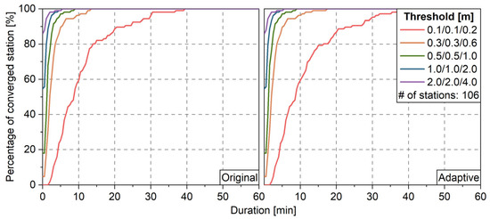
Figure 9.
Percentage of converged stations without (left) and with (right) ASM.
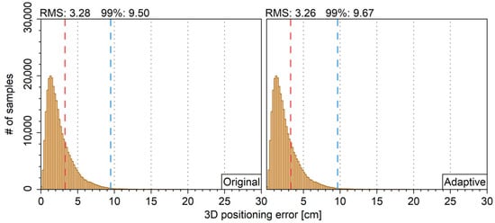
Figure 10.
Hists for 3D positioning error without (left) and with (right) ASM.
3.2.2. PPP Results for Unsuitable Stochastic Model
The results for the IGS station TONG are specifically analyzed, which is the only station whose observational errors are obviously larger than other stations. Figure 11 shows the estimated observational variance factors. The factors for pseudo-range and carrier-phase observations are about 0.6 m and 6 mm, respectively, which are larger than other stations. Though the exact cause for the large factors remains unknown, enhancing the stochastic model could still be beneficial to the performance. Figure 12 shows the positioning errors with and without the ASM and Table 2 shows the RMSs of positioning errors on east, north, and up directions after convergence. Note that the stochastic model for results without the ASM is the same as those in Section 3.2.1. The positioning precision is improved with the help of the ASM for 57%, 51%, and 25% for east, north, and up directions. It shows that when the predetermined stochastic model is unsuitable, the ASM can be adjusted according to the actual statistical properties of the observational noise and improve the positioning performance. Unfortunately, the data quality for most IGS stations is good, and it is difficult to find another example to prove the benefits of ASM to PPP float solutions. Non-IGS data under bad observational conditions is needed for future study.
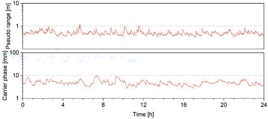
Figure 11.
Estimated pseudo-range and carrier-phase variance factors for TONG station.
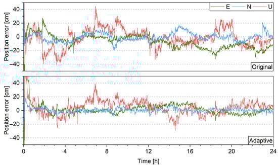
Figure 12.
Positioning error for TONG station without (top) and with (bottom) ASM.
Table 2.
RMS of the position errors for TONG station.
To further show the benefits of the ASM, PPP without an ASM is carried out again for the TONG station with standard deviations of pseudo-range and carrier-phase observations as 0.6 m and 6 mm, whose positioning error is shown in Figure 13. The result is different from the top panel of Figure 12 while similar to the bottom panel, which shows that the positioning performance is improved when the stochastic model is adjusted. This proves that the benefits of the ASM to positioning come from the ability of adjusting the stochastic model on-the-fly.
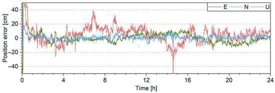
Figure 13.
Positioning error for TONG station with standard deviations of pseudo-range and carrier-phase observations as 0.6 m and 6 mm.
3.3. PPP-AR Test
Besides PPP float solution, ambiguity resolution is also influenced by the stochastic model, which will be analyzed in this section. The ambiguity resolution with the Integer Bootstrapping (IB) strategy will be introduced first; then, the performance of PPP-AR with an ASM will be analyzed.
3.3.1. Ambiguity Resolution
The IB strategy is a widely used ambiguity resolution strategy which fixes one ambiguity at a time and corrects the remaining float ambiguities with the fixed one [45]. For integer ambiguity parameter and its float estimation with variance matrix , the th ambiguity is fixed with the IB strategy as
where is corrected with the fixed solution of its previous ambiguities, i.e., under the conditions of . The recursive evaluation equation for reads
where and are and corrected with the fixed solution of the previous ambiguities, is the entry on the th row and th column of and is the th diagonal entry of . For arbitrary , , and that , , , and hold, where is the number of ambiguities, one has
where for , one has and .
3.3.2. PPP-AR Results for Global Stations
The ambiguity parameters of PPP are not integer due to the existence of phase biases of the satellites and receiver. To obtain ambiguities with integer properties, the satellite phase biases need to be corrected with IGS product and single difference should be applied between satellites to eliminate receiver phase biases. The BIA product from CODE is used to correct the satellite phase biases [41]. Due to the lack of a BDS phase bias product, only the ambiguities of GPS and Galileo are fixable. The AR process starts with float solutions of ambiguities and the corresponding variance matrix. Z-transformation is applied to obtain decorrelated ambiguities. Then, the widely used partial AR (PAR) procedure with the IB strategy is conducted, where a subset of decorrelated ambiguities is selected with a success rate threshold of 99.99% [29,46,47,48]. Finally, the position parameters are corrected with the fixed decorrelated ambiguities. Figure 14 shows the GPS+Galileo PPP-AR positioning errors for IGS stations AJAC, CHPG, and FAIR. The plots in the left and the right panels are very similar, which shows the ASM has little impact on the performance of PPP-AR.
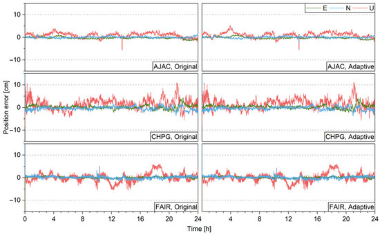
Figure 14.
PPP-AR positioning errors without (left) and with (right) ASM.
With the solutions of all stations, Figure 15 shows the hists for 3D positioning errors. The plots for results with the ASM are similar to those without the ASM, which also happens to the float solution. This shows that, if the stochastic model is suitable, the ASM is not beneficial to the performance of PPP-AR.
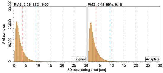
Figure 15.
Hist for PPP-AR 3D positioning error without (left) and with (right) ASM.
3.3.3. PPP-AR Results for Unsuitable Stochastic Model
The results for IGS station TONG are specifically analyzed, whose observational errors are larger than other stations, as is shown in Section 3.2.2. Figure 16 shows the PPP-AR positioning errors for the TONG station and the RMSs on three directions are given in Table 3. With the ASM, the positioning errors on east, north, and up directions are reduced for 36%, 28%, and 36%, respectively. This shows when the predetermined stochastic model is unsuitable, an ASM can enhance the performance of PPP-AR greatly.
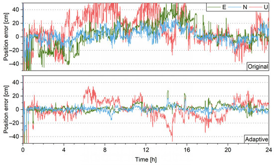
Figure 16.
PPP-AR positioning error for TONG station without (top) and with (bottom) ASM.
Table 3.
RMS of the PPP-AR position errors for TONG station.
To further show the benefits of the ASM, PPP-AR without an ASM is carried out again for the TONG station with standard deviations of pseudo-range and carrier-phase observations as 0.6 m and 6 mm, whose positioning error is shown in Figure 17. The result is better than the top panel of Figure 16 while slightly worse than the bottom panel, which shows the benefits of the ASM to positioning come from the ability of adjusting the stochastic model on-the-fly.
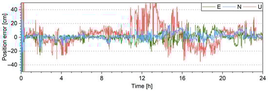
Figure 17.
PPP-AR positioning error for TONG station with standard deviations of pseudo-range and carrier-phase observations as 0.6 m and 6 mm.
3.4. Tests on Cycle-Slip Detection
The detection of unmodeled bias with DIA is another algorithm that could benefit from an ASM. DIA could use all the redundant information and construct an optimal procedure for anomaly detection [32]. Since DIA uses the stochastic model, it can show the ability of an ASM to enhance the detection effectiveness when the predefined stochastic model is improper. Among the anomalies of PPP, the cycle slip is the most important one due to its impact on positioning; therefore, cycle-slip detection with DIA will be tested to examine the benefit of the ASM. The DIA algorithm will be introduced; then, the PPP cycle-slip detection with DIA will be designed; finally, the performance will be analyzed.
3.4.1. DIA Algorithm
For an arbitrary observational model
where , one has the least square estimation (LSQ)
where and form the normal equation . The estimated value of the LSQ residual reads
where , . Equation (32) is also known as the null hypothesis. When there is unmodeled bias in the observational model, one has the alternative hypothesis
where is the unmodeled bias parameter with corresponding design matrix . Since Equation (35) is solved without considering , the solution of Equation (35) reads
where . This shows that the unmodeled bias is absorbed by both and , causing both increased positioning error and a larger residual. Note that there could be different types of unmodeled biases. The DIA algorithm is carried out in three steps: it determines whether there is unmodeled bias in the detection step, distinguishes what type of bias it is in the identification step, and finally modifies the observational model to include the unmodeled bias for better positioning performance in the adaptation step. For the detection, an overall test for determining whether there is unmodeled bias is carried out as
where is the upper α-quantile of a central chi-squared distribution with degrees of freedom, α is the false alarm probability of the overall test, and is the rank of the residual estimation. If Equation (38) holds, there is unmodeled bias during the observation, which needs to be identified. For the identification with different alternative hypothesis, is calculated for the th alternative hypothesis as
where , . When the dimensions of each are the same, the alternative hypothesis with the biggest is selected as the most likely one. Finally for the adaptation, the solution and its variance matrix are updated as
where , .
3.4.2. PPP Cycle-Slip Detection with DIA
To detect cycle slip with DIA, the model of the Kalman filter should be expressed in the form of Equation (32) and the alternative hypothesis for cycle slip should be designed. With the estimated system state at epoch in Equation (7), dynamic model in Equation (5), and observational model in Equation (6), the single-epoch model of the Kalman filter can be summarized as
The alternative hypothesis for the dynamic model with unmodeled bias reads
where is a unit vector with the th entry as 1, and is the bias that introduced for the th parameter of . To detect the cycle slip, an alternative hypothesis in the form of Equation (42) is set up for each ambiguity parameter of PPP, where is actually the cycle-slip parameter. Then, DIA algorithm is applied to detect the cycle slip.
3.4.3. Results for the Cycle-Slip Detection
The test is carried out for observational data with simulated cycle slips. For the observation of each station, two carrier-phase observations are randomly selected every 10 min and simulated with cycle slips of one cycle. Note that the observations are modified for not only the epoch that the cycle slips happen in but also subsequent epochs. GPS + BDS + Galileo PPP is performed for global stations with DIA detecting the simulated cycle slips, where either a predefined stochastic model or an ASM is used. Figure 17 shows the positioning error for the IGS station AJAC. Without the ASM, the positioning error degrades due to some undetected cycle slips; with the help of the ASM, the positioning error looks normal and free of undetected cycle slips. The main reason could be that the enhanced stochastic model for ionospheric delay makes the detection with dual-frequency data easier.
Figure 18 shows the hists for 3D positioning error. Though not comparable with those without simulated cycle slips, the positioning error of the ASM is dramatically reduced compared with that of the predefined stochastic model. Table 4 shows the numbers of simulated and detected cycle slips of all stations. The detection rate is improved from 81% to 92% with the help of the ASM, which indeed shows that the enhanced stochastic model is helpful to cycle-slip detection.
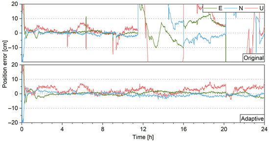
Figure 18.
PPP positioning error with simulated cycle slips which are detected with DIA.
Table 4.
Numbers of simulated and detected cycle slips.
3.5. Tests on Reconvergence and Interruption Repair
The reconvergence and interruption repair of PPP after data interruption are also influenced by the stochastic model. Here the interruption means all satellites are not visible for a few minutes and then reappear, which could happen in a city environment. Direct reconvergence is the basic method for handling interrupted data, which is to keep the parameters of the satellites and continue updating them once the satellites reappear. However, the ambiguities have to be reset due to the interrupted tracking of carrier-phase signals, whose reconvergences take dozens of minutes. Furthermore, the difference between the ambiguities before and after the interruption is actually a cycle-slip parameter with integer properties, which could be fixed with AR algorithm to accelerate the reconvergence [49,50,51,52,53]. The latter method is called interruption repair. The direct reconvergence requires a reliable time update of the filter to preserve the information, which would require a suitable stochastic model; the interruption repair is based on the AR algorithm, which is also influenced by the stochastic model. The variance factor of ionospheric delay is the only time-variant factor among all factors. The enhanced stochastic model of ionospheric delay should be beneficial to convergence. Unfortunately, the estimated factor also takes time to converge, which makes the ASM not beneficial to the convergence. However, the factor is already converged when interruptions occur; therefore, the stochastic model of ionospheric delay refined with an ASM could be beneficial to reconvergence and interruption repair, which will be tested in this section.
3.5.1. Reconvergences After 3 Min Interruptions
For the observation data of each station, 3 min of data interruptions are simulated every 2 h by simply removing all observations during the interruptions. GPS PPP tests are carried out, where the ionospheric delay parameters are kept during the interruption while ambiguity parameters are reset. Figure 19 shows the positioning errors for the IGS station BUCU. For data segments such as 2~4, 4~6, and 6~8, the ASM improves the reconvergence. This is mainly because of the enhanced stochastic model for ionospheric delay. Figure 20 shows the percentage of reconverged data segments for all stations. The time for 60% of the segments to reconverge to the threshold of 0.1/0.1/0.2 m is reduced from 19 min to 15.5 min, showing the benefits of ASM.
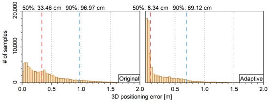
Figure 19.
Hists for 3D positioning error with simulated cycle slips which are detected with DIA.
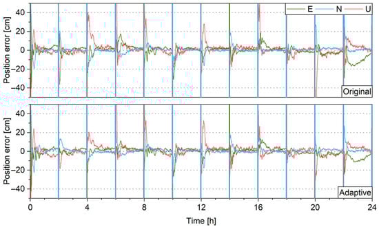
Figure 20.
PPP positioning errors with 3 min data interruptions every 2 h, without (top) and with (bottom) ASM.
To show the impact of refined ionospheric stochastic model to reconvergence, Figure 21 shows the PPP positioning errors for the IGS station BUCU where ionospheric delay is modeled as white noise process. It shows that, as the model of ionospheric delay cannot be enhanced by the ASM, the reconvergence is not improved at all.
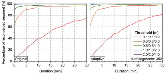
Figure 21.
Percentage of reconverged data segments without (left) and with (right) ASM.
3.5.2. Interruption Repair for 3 Min Interruptions
The algorithm for repairing interruption will be introduced first. The basic idea is to fix the cycle slip between the ambiguity before the interruption and the one after the interruption. The ionospheric delay and ambiguity parameters of all satellites are kept during the interruption. Once the satellites reappear, new ambiguity parameters are introduced and updated during the filter update. Then cycle slips are derived from the ambiguities before the interruption and the newly introduced one. The ambiguity resolution method in Section 3.3 is applied to the cycle-slip parameters and the system state is updated with the fixed cycle slips. This attempt of repairing repeats for each subsequent epoch. After 30 min, the ambiguities before the interruption are removed and the remaining “float” cycle slips will not be fixed anymore. Since the cycle slips are obtained via subtraction between old and new ambiguities, positive correlation between ambiguities would yield more precise and easy-to-fix cycle slips. With the ionospheric information preserved, the new ambiguity is linked with the old one through ionospheric parameters; therefore, the ASM could help the repair through precise modeling of the ionospheric delay.
PPP tests are carried out for global stations with interruption repair. Figure 22 shows the positioning errors with interruption repair for the IGS station CPVG. With the predefined stochastic model, at least six data segments are not repaired; while with the ASM, only two data segments are not repaired and the remaining segments instantly reconverge once the satellites reappear. This shows that with the ionospheric model refined, the repair of interruption becomes more effective. Finally, Figure 23 shows the percentage of reconverged data segments for all stations. The time for 80% of the segments to converge to the threshold of 0.1/0.1/0.2 m is greatly reduced from 30 min to 13.5 min, which proves the enhanced ionospheric stochastic model is indeed beneficial to the interruption repair.
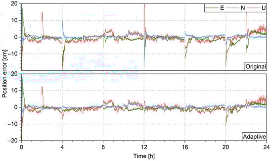
Figure 22.
PPP positioning errors with interruption repair, without (top) and with (bottom) ASM.
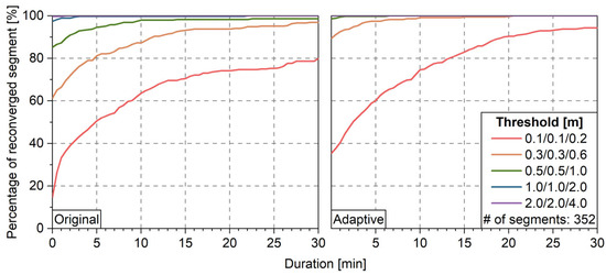
Figure 23.
Percentage of reconverged data segments with interruption repair, without (left) and with (right) ASM.
4. Discussion
An adaptive stochastic model (ASM) significantly enhances various aspects of Precise Point Positioning (PPP), necessitating a comprehensive assessment of its benefits. This paper implements an ASM by integrating the least-squares variance component estimation (LS-VCE) algorithm with the Kalman filter model and evaluates its contributions to PPP performance from multiple perspectives, including observational condition reflection, PPP float and fixed solutions, cycle-slip detection using DIA, reconvergence, and interruption repair. The main findings demonstrate that the ASM effectively improves the observational variance matrix when the predefined model is inadequate, benefiting both PPP float and fixed solutions. Additionally, the ASM enhances the ionospheric stochastic model, captures its temporal variations, and contributes to higher DIA success rates, faster reconvergence after data interruptions, and improved interruption repair. The detailed conclusions are summarized as follows:
- Variance Factor Estimation: Variance factors for the observational noise of pseudo-range and carrier-phase measurements are estimable and capture time-varying observational conditions. The variance factor for the ionospheric delay process noise is estimable and reflects the temporal variation of the ionosphere. The variance factor for tropospheric delay is not estimable due to its minimal variation between epochs, which is overwhelmed by the noise.
- PPP Float and Fixed Solutions: The ASM offers no significant advantage when the predefined stochastic model is appropriate. However, when observational noise is large, rendering the predefined model unsuitable, the ASM adjusts the variance factors to deliver superior PPP float and fixed solutions.
- Cycle-Slip Detection with DIA: With the predefined stochastic model, 19% of simulated cycle slips remain undetected, resulting in degraded positioning precision at the meter level. With the ASM, the undetected cycle slips are reduced to 8%, and positioning precision improves. Notably, the 50th percentile error is reduced by 75%.
- Reconvergence and Interruption Repair: Simulated 3 min data interruptions every 2 h reveal that the ASM reduces the reconvergence time for 60% of data segments to a threshold of 0.1/0.1/0.2 m from 19 min (predefined stochastic model) to 15.5 min. This improvement is attributed to the enhanced variance factor for ionospheric delay process noise. Interruption repair tests show that reconvergence time for 80% of segments to the same threshold decreases from 30 min (predefined stochastic model) to 13.5 min (ASM), underscoring the benefits of the improved ionospheric stochastic model.
In summary, the adaptive stochastic model not only refines variance factor estimation to reflect observational conditions but also significantly enhances PPP float and fixed solutions under challenging conditions, improves cycle-slip detection, and accelerates reconvergence and interruption repair. These findings highlight the broad applicability and effectiveness of an ASM in improving PPP performance. However, the IGS stations used for our tests are mostly under good observational conditions. The ASM will be tested for challenging applications such as maritime positioning in the future to show its ability to improve positioning in poor observational conditions.
Author Contributions
Methodology, Y.Z. (Yanning Zheng) and Y.S.; software, Y.Z. (Yanning Zheng); validation, Y.Z. (Yanning Zheng), Y.Z. (Yubin Zhou), and S.W.; resources, Y.S. and Y.Z. (Yubin Zhou); writing—original draft preparation, Y.Z. (Yanning Zheng) and Y.L.; writing—review and editing, Y.S. and S.W.; funding acquisition, Y.Z. (Yubin Zhou). All authors have read and agreed to the published version of the manuscript.
Funding
This research was supported by the Key Project of Marine Service Industry in Shandong Province (37000025050809990005X).
Data Availability Statement
The data presented in this study are available on the IGS data server of ESA at ftp://gssc.esa.int (accessed on 12 August 2024).
Conflicts of Interest
The authors declare no conflicts of interest.
References
- Zumberge, J.F.; Heflin, M.B.; Jefferson, D.C.; Watkins, M.M.; Webb, F.H. Precise Point Positioning for the Efficient and Robust Analysis of GPS Data from Large Networks. J. Geophys. Res. 1997, 102, 5005–5017. [Google Scholar] [CrossRef]
- Jin, S.; Wang, J.; Park, P.-H. An Improvement of GPS Height Estimations: Stochastic Modeling. Earth Planets Space 2005, 57, 253–259. [Google Scholar] [CrossRef]
- Li, Y.; Li, B.; Gao, Y. Improved PPP Ambiguity Resolution Considering the Stochastic Characteristics of Atmospheric Corrections from Regional Networks. Sensors 2015, 15, 29893–29909. [Google Scholar] [CrossRef] [PubMed]
- Li, B.; Lou, L.; Shen, Y. GNSS Elevation-Dependent Stochastic Modeling and Its Impacts on the Statistic Testing. J. Surv. Eng. 2016, 142, 04015012. [Google Scholar] [CrossRef]
- Li, B.; Zhang, L.; Verhagen, S. Impacts of BeiDou Stochastic Model on Reliability: Overall Test, w-Test and Minimal Detectable Bias. GPS Solut. 2017, 21, 1095–1112. [Google Scholar] [CrossRef]
- Yang, L.; Li, B.; Li, H.; Rizos, C.; Shen, Y. The Influence of Improper Stochastic Modeling of Beidou Pseudoranges on System Reliability. Adv. Space Res. 2017, 60, 2680–2690. [Google Scholar] [CrossRef]
- Zaminpardaz, S.; Teunissen, P.J.G. DIA-Datasnooping and Identifiability. J. Geod. 2019, 93, 85–101. [Google Scholar] [CrossRef]
- Kim, D.; Langley, R.B. GPS Ambiguity Resolution and Validation: Methodologies, Trends and Issues. In Proceedings of the 7th GNSS Workshop–International Symposium on GPS/GNSS, Seoul, Korea, 30 November–2 December 2000. [Google Scholar]
- Amiri-Simkooei, A.R.; Jazaeri, S.; Zangeneh-Nejad, F.; Asgari, J. Role of Stochastic Model on GPS Integer Ambiguity Resolution Success Rate. GPS Solut. 2016, 20, 51–61. [Google Scholar] [CrossRef]
- Han, S. Quality-Control Issues Relating to Instantaneous Ambiguity Resolution for Real-Time GPS Kinematic Positioning. J. Geod. 1997, 71, 351–361. [Google Scholar] [CrossRef]
- Mehra, R. Approaches to Adaptive Filtering. IEEE Trans. Automat. Contr. 1972, 17, 693–698. [Google Scholar] [CrossRef]
- Chin, L. Advances in Adaptive Filtering. In Control and Dynamic Systems, Advanced in Theory and Applications; Leondes, C.T., Ed.; Elsevier: Amsterdam, The Netherlands, 1979; Volume 15, pp. 277–356. [Google Scholar]
- Zhu, Z.; Liu, S. An Improved Sage-Husa Adaptive Filtering Algorithm. In Proceedings of the 31st Chinese Control Conference, Hefei, China, 25–27 July 2012; pp. 5113–5117. [Google Scholar]
- Xu, T.; Xu, X.; Xu, D.; Zou, Z.; Zhao, H. A New Robust Filtering Method of GNSS/MINS Integrated System for Land Vehicle Navigation. IEEE Trans. Veh. Technol. 2022, 71, 11443–11453. [Google Scholar] [CrossRef]
- Elzoghby, M.; Arif, U.; Li, F.; Zhi Yu, X. Investigation of Adaptive Robust Kalman Filtering Algorithms for GPS/DR Navigation System Filters. IOP Conf. Ser. Mater. Sci. Eng. 2017, 187, 012019. [Google Scholar] [CrossRef]
- Xu, S.; Zhou, H.; Wang, J.; He, Z.; Wang, D. SINS/CNS/GNSS Integrated Navigation Based on an Improved Federated Sage–Husa Adaptive Filter. Sensors 2019, 19, 3812. [Google Scholar] [CrossRef]
- Zhou, Z.; Shen, Y.; Li, B. Stochastic Model of GPS Doppler: Evaluation, Modeling and Performance. In China Satellite Navigation Conference (CSNC) 2012 Proceedings; Sun, J., Liu, J., Yang, Y., Fan, S., Eds.; Lecture Notes in Electrical Engineering; Springer: Berlin/Heidelberg, Germany, 2012; Volume 159, pp. 395–406. ISBN 978-3-642-29186-9. [Google Scholar]
- Li, B.; Hao, Q. Towards Reliable and Precise BeiDou Positioning with Stochastic Modelling. In International Symposium on Earth and Environmental Sciences for Future Generations; Freymueller, J.T., Sánchez, L., Eds.; International Association of Geodesy Symposia; Springer International Publishing: Cham, Switzerland, 2016; Volume 147, pp. 229–235. ISBN 978-3-319-69169-5. [Google Scholar]
- Li, B. Stochastic Modeling of Triple-Frequency BeiDou Signals: Estimation, Assessment and Impact Analysis. J. Geod. 2016, 90, 593–610. [Google Scholar] [CrossRef]
- Hu, H.; Zhou, F.; Jin, S. Improved Stochastic Modeling of Multi-GNSS Single Point Positioning with Additional BDS-3 Observations. Meas. Sci. Technol. 2021, 32, 045105. [Google Scholar] [CrossRef]
- Wang, J.-G.; Gopaul, N.; Scherzinger, B. Simplified Algorithms of Variance Component Estimation for Static and Kinematic GPS Single Point Positioning. J. Glob. Position. Syst. 2009, 8, 43–52. [Google Scholar] [CrossRef]
- Zhang, X.; Lu, X. Online Algorithm for Variance Components Estimation. Commun. Nonlinear Sci. Numer. Simul. 2021, 97, 105722. [Google Scholar] [CrossRef]
- Hou, P.; Zha, J.; Liu, T.; Zhang, B. LS-VCE Applied to Stochastic Modeling of GNSS Observation Noise and Process Noise. Remote Sens. 2022, 14, 258. [Google Scholar] [CrossRef]
- Zhang, Q.; Zhao, L.; Zhou, J. A Novel Weighting Approach for Variance Component Estimation in GPS/BDS PPP. IEEE Sens. J. 2019, 19, 3763–3771. [Google Scholar] [CrossRef]
- Zhang, Q.; Zhao, L. Adaptive Stochastic Model Based on LS-VCE for Observations in Kinematic Precise Point Positioning. In Proceedings of the 2022 41st Chinese Control Conference (CCC), Hefei, China, 25–27 July 2022; IEEE: Piscataway, NJ, USA, 2022; pp. 3410–3414. [Google Scholar]
- Yang, X.; Chang, G.; Wang, Q.; Zhang, S.; Mao, Y.; Chen, X. An Adaptive Kalman Filter Based on Variance Component Estimation for a Real-Time ZTD Solution. Acta Geod. Geophys. 2019, 54, 89–121. [Google Scholar] [CrossRef]
- Chang, G.; Xu, T.; Yao, Y.; Wang, Q. Adaptive Kalman Filter Based on Variance Component Estimation for the Prediction of Ionospheric Delay in Aiding the Cycle Slip Repair of GNSS Triple-Frequency Signals. J. Geod. 2018, 92, 1241–1253. [Google Scholar] [CrossRef]
- Teunissen, P.J.G. Least-Squares Estimation of the Integer GPS Ambiguities. In Invited Lecture. Section IV Theory and Methodology, IAG General Meeting, Beijing, China; Delft Geodetic Computing Centre: Delft, The Netherlands, 1993. [Google Scholar]
- Psychas, D.; Verhagen, S.; Teunissen, P.J.G. Precision Analysis of Partial Ambiguity Resolution-Enabled PPP Using Multi-GNSS and Multi-Frequency Signals. Adv. Space Res. 2020, 66, 2075–2093. [Google Scholar] [CrossRef]
- De Jonge, P.; Tiberius, C.C.J.M. The LAMBDA Method for Integer Ambiguity Estimation: Implementation Aspects; Publications of the Delft Computing Centre, LGR-Series; Delft Computing Centre: Delft, The Netherlands, 1996; Volume 12, pp. 1–47. [Google Scholar]
- Verhagen, S.; Li, B.; Teunissen, P.J.G. Ps-LAMBDA: Ambiguity Success Rate Evaluation Software for Interferometric Applications. Comput. Geosci. 2013, 54, 361–376. [Google Scholar] [CrossRef]
- Baarda, W. A Testing Procedure for Use in Geodetic Networks; Netherlands Geodetic Commission: Amersfoort, The Netherlands, 1968; Volume 2. [Google Scholar]
- Chen, D. A Method for the Repair of Cycle Slip Using Double-Differenced Velocity Estimation for GNSS RTK Positioning. Adv. Space Res. 2019, 63, 2809–2821. [Google Scholar] [CrossRef]
- Momoh, J.A. Robust GNSS Point Positioning in the Presence of Cycle Slips and Observation Gaps. Ph.D. Thesis, University College London, London, UK, 2013. [Google Scholar]
- Li, B.; Qin, Y.; Liu, T. Geometry-Based Cycle Slip and Data Gap Repair for Multi-GNSS and Multi-Frequency Observations. J. Geod. 2019, 93, 399–417. [Google Scholar] [CrossRef]
- Rao, C.R. Estimation of Variance and Covariance Components-MINQUE Theory. J. Multivar. Anal. 1971, 1, 257–275. [Google Scholar] [CrossRef]
- Koch, K. Schätzung von Varianzkomponenten. Allg. Vermess. Nachrich. 1978, 85, 264–269. [Google Scholar]
- Teunissen, P.J.G.; Amiri-Simkooei, A.R. Least-Squares Variance Component Estimation. J. Geod. 2008, 82, 65–82. [Google Scholar] [CrossRef]
- Zhang, B.; Hou, P.; Liu, T.; Yuan, Y. A Single-Receiver Geometry-Free Approach to Stochastic Modeling of Multi-Frequency GNSS Observables. J. Geod. 2020, 94, 37. [Google Scholar] [CrossRef]
- Teunissen, P.J.G. Zero Order Design: Generalized Inverses, Adjustment, the Datum Problem and S-Transformations. In Optimization and Design of Geodetic Networks; Grafarend, E.W., Sansò, F., Eds.; Springer: Berlin/Heidelberg, Germany, 1985; pp. 11–55. ISBN 978-3-642-70661-5. [Google Scholar]
- Schaer, S.; Villiger, A.; Arnold, D.; Dach, R.; Prange, L.; Jäggi, A. The CODE Ambiguity-Fixed Clock and Phase Bias Analysis Products: Generation, Properties, and Performance. J. Geod. 2021, 95, 81. [Google Scholar] [CrossRef]
- Su, K.; Jiao, G. Estimation of BDS Pseudorange Biases with High Temporal Resolution: Feasibility, Affecting Factors, and Necessity. Satell. Navig. 2023, 4, 17. [Google Scholar] [CrossRef]
- de Lacy, M.C.; Reguzzoni, M.; Sansò, F.; Venuti, G. The Bayesian Detection of Discontinuities in a Polynomial Regression and Its Application to the Cycle-Slip Problem. J. Geod. 2008, 82, 527–542. [Google Scholar] [CrossRef]
- Cai, C.; Liu, Z.; Xia, P.; Dai, W. Cycle Slip Detection and Repair for Undifferenced GPS Observations under High Ionospheric Activity. GPS Solut. 2013, 17, 247–260. [Google Scholar] [CrossRef]
- Teunissen, P.J.G. GNSS Ambiguity Bootstrapping: Theory and Application. In Proceedings of the International Symposium on Kinematic Systems in Geodesy, Geomatics and Navigation, Banff, AB, Canada, 5–8 June 2001; pp. 246–254. [Google Scholar]
- Teunissen, P.J.G. An Optimality Property of the Integer Least-Squares Estimator. J. Geod. 1999, 73, 587–593. [Google Scholar] [CrossRef]
- Odijk, D.; Arora, B.S.; Teunissen, P.J.G. Predicting the Success Rate of Long-Baseline GPS+Galileo (Partial) Ambiguity Resolution. J. Navig. 2014, 67, 385–401. [Google Scholar] [CrossRef]
- Nardo, A.; Li, B.; Teunissen, P.J.G. Partial Ambiguity Resolution for Ground and Space-Based Applications in a GPS+Galileo Scenario: A Simulation Study. Adv. Space Res. 2016, 57, 30–45. [Google Scholar] [CrossRef]
- Dai, Z.; Knedlik, S.; Loffeld, O. Instantaneous Triple-Frequency GPS Cycle-Slip Detection and Repair. Int. J. Navig. Obs. 2009, 2009, 407231. [Google Scholar] [CrossRef]
- Zhang, W.; Wang, J. A Real-Time Cycle Slip Repair Method Using the Multi-Epoch Geometry-Based Model. GPS Solut. 2021, 25, 60. [Google Scholar] [CrossRef]
- Zhang, Z.; Zeng, J.; Li, B.; He, X. Principles, Methods and Applications of Cycle Slip Detection and Repair under Complex Observation Conditions. J. Geod. 2023, 97, 50. [Google Scholar] [CrossRef]
- Zhang, X.; Li, X. Instantaneous Re-Initialization in Real-Time Kinematic PPP with Cycle Slip Fixing. GPS Solut. 2012, 16, 315–327. [Google Scholar] [CrossRef]
- Yao, Y.-F.; Gao, J.-X.; Wang, J.; Hu, H.; Li, Z.-K. Real-Time Cycle-Slip Detection and Repair for BeiDou Triple-Frequency Undifferenced Observations. Surv. Rev. 2016, 48, 367–375. [Google Scholar] [CrossRef]
Disclaimer/Publisher’s Note: The statements, opinions and data contained in all publications are solely those of the individual author(s) and contributor(s) and not of MDPI and/or the editor(s). MDPI and/or the editor(s) disclaim responsibility for any injury to people or property resulting from any ideas, methods, instructions or products referred to in the content. |
© 2025 by the authors. Licensee MDPI, Basel, Switzerland. This article is an open access article distributed under the terms and conditions of the Creative Commons Attribution (CC BY) license (https://creativecommons.org/licenses/by/4.0/).