Article

Evolution and Attribution Analysis of the Relationship Among Soil Erosion Negative Service, Carbon Sequestration, and Water Yield in the Yellow River Basin After the Grain for Green Program

1
College of Surveying and Geo-Informatics, North China University of Water Resources and Electric Power, Zhengzhou 450046, China
2
School of Water Conservancy, North China University of Water Resources and Electric Power, Zhengzhou 450046, China
3
Key Research Institute of Yellow River Civilization and Sustainable Development & Yellow River Civilization by Provincial and Ministerial Co-Construction of Collaborative Innovation Center, Henan University, Kaifeng 475001, China
4
Institute of Soil and Water Conservation, Northwest A&F University, Yangling 712100, China
5
Jinan Water Supply and Drainage Monitoring Center, Jinan 250000, China
*
Author to whom correspondence should be addressed.
Remote Sens. 2025, 17(17), 3028; https://doi.org/10.3390/rs17173028
Submission received: 2 July 2025 / Revised: 21 August 2025 / Accepted: 21 August 2025 / Published: 1 September 2025

Abstract

Understanding the tradeoff and synergy among ecosystem services (ESs) and their influencing factors is a prerequisite for simultaneously managing multiple ESs and holds significant importance for achieving harmonious regional development between humans and nature. Existing research predominantly focuses on the overall characteristics of tradeoff and synergy, while studies on spatially differentiated tradeoff and synergy characteristics remain limited. In addition, their driving mechanisms are not yet fully understood, especially in large-scale river basins. This study, taking the Yellow River Basin (YRB) from 2000 to 2023 as the study area, employed multi-source data and multiple models to quantify three ESs, including soil erosion negative service (indirectly reflecting the soil conservation service function), carbon sequestration, and water yield. Combining Pearson correlation analysis, a geographically weighted regression model, and optimal parameter geographical detection, we identified the spatiotemporal interaction relationships and their dominant drivers. The results indicated that soil erosion negative services decreased by 24.89%, while carbon sequestration and water yield increased by 53.30% and 38.47%, respectively. The most significant improvements in the three ESs were observed in the midstream of the YRB. Spatially, soil erosion negative service decreased from west to east. Carbon sequestration exhibited a spatial pattern of higher values in the south and east and lower values in the north and west. Water yield decreased from south to north. Tradeoff relationships existed between soil erosion negative service and carbon sequestration and between soil erosion negative service and water yield. A synergistic relationship existed between carbon sequestration and water yield. Over time, the proportion of areas showing synergy among these three ESs decreased. However, synergistic areas remained more common than tradeoff areas. This was especially evident in the relationship between carbon sequestration and water yield, where synergy consistently accounted for over 78% of the YRB. Rainfall, soil properties, and fractional vegetation cover were identified as important drivers of the tradeoff/synergy between soil erosion negative service and carbon sequestration. Rainfall, temperature, fractional vegetation cover, and elevation were significant drivers of the interactions between carbon sequestration and water yield. Population density, fractional vegetation cover, GDP density, and rainfall were the main influencing factors for the tradeoff/synergy between soil erosion negative service and water yield. Our general methodology and results provide valuable decision-making references for policymakers, highlighting the necessity of considering the spatiotemporal heterogeneity in ESs tradeoff characteristics and their underlying driving factors.

1. Introduction

As ecosystem services (ESs) become increasingly relevant to human well-being [1,2], it is significant to incorporate ESs into the formulation of ecosystem management strategies [3,4]. It has been proven that ecosystem health is deteriorating at an unprecedented rate, destroying the foundation of human livelihoods and adversely affecting quality of life [2,5]. In this context, it is urgent to adopt management strategies that incorporate the sustainable use of ESs. The main factors hindering this progress relate to unraveling the complex tradeoff/synergy relationships among different ESs and how different socio-ecological factors affect these relationships [6,7]. A full understanding of such interaction relationships and the associated drivers is essential for designing environmental management strategies that simultaneously improve multiple ESs to enhance human well-being [8,9].
Correctly understanding the complex interaction relationships among various ESs is a prerequisite for achieving sustainable ecosystem management [10,11]. Due to the diver-sity of ESs, the uneven spatial distribution, and the selectivity of human use, the relation-ships between ESs exhibit changes such as tradeoffs (where one service increases at the expense of another) and synergies (where services mutually enhance each other) under the combined influence of multiple factors [12]. Currently, numerous scholars domestically and internationally have actively explored tradeoff and synergy relationships among ESs, yielding substantial achievements. In terms of research content, these include the qualita-tive identification [13], quantitative analysis [14], supply–demand tradeoffs [15], and driving factors and mechanisms [16,17] of ES tradeoffs/synergies. Methodologically, stud-ies employ statistical methods [7], spatial analysis [18], scenario simulation analysis [19,20], cluster analysis [21], and the service flow approach [22]. Regarding research scale, studies initially focused predominantly on small-scale areas with relatively homogeneous geographical conditions, such as administrative units at the provincial, city, or county level [14,20,23]. Subsequently, it gradually expanded to complex geographical units in-fluenced by multiple factors, such as small basins and ecological functional zones [22,24]. Overall, these studies play a crucial role in supporting the in-depth analysis of ecological issues and subsequently formulating management strategies. However, existing research predominantly focuses on the overall tradeoff/synergy relationships of ESs, including the examination at different scales [25]. Until recently, scholars gradually realized that such overall relationships may mask local spatial variations [26,27]. Consequently, scholars now pay attention to spatial interactions [23,25]. However, due to the complexity and di-versity of the socioecological conditions within the regions, especially within large river basins, the spatial interactions will have different manifestation characteristics. Therefore, further studies are needed to support certain regions in more targeted efforts to alleviate tradeoffs and enhance synergies.
Simultaneously, building on the exploration of ESs tradeoff/synergy relationships, identifying the key factors influencing these relationship dynamics is a prerequisite for subsequent implementation of ecosystem improvement and protection [9]. Some studies have chosen methods such as traditional regression analysis [27] or geographically weighted regression (GWR) [13] to analyze the driving factors of ES changes. However, regression methods must meet classical regression assumptions. In addition, these meth-ods are prone to endogeneity issues arising from potential reverse causality between in-dependent and dependent variables. The optimal parameter geographical detector (OPGD) can quantitatively analyze the explanatory power of factors on dependent variables. It can also address the issue of spatial discretization of continuous variables and is an efficient tool for detecting the spatial heterogeneity of geographical phenomena [28]. This method not only effectively avoids endogeneity problems inherent in regression analysis but is al-so suitable for analyzing both numerical and qualitative data [29]. These advantages pro-vide a robust tool for accurately revealing the driving mechanisms behind ESs interac-tions.
The Yellow River Basin (YRB), as China’s second-largest river basin, serves as an ecological corridor connecting the Qinghai–Tibet Plateau, the Loess Plateau, and the North China Plain. It constitutes an extremely important ecological security barrier for the country and bears significant ESs functions [30]. However, under the long-term influence of human activities, the YRB suffers from a poor ecological foundation and severe vegeta-tion degradation. In addition, it is facing a series of problems including water scarcity, se-rious soil erosion, and fragile ecological environments [31,32]. Against this backdrop, ex-ploring how to protect the ecological environment of the YRB and achieve regional sus-tainable development is a core component of the national major strategy for ecological protection and high-quality development of the YRB [33]. In light of this, this study takes the YRB as the case study area. Comprehensively considering the urgent needs for ecolog-ical protection and ESs improvement within the basin [32,33,34], we selected three key ESs—soil erosion negative service, carbon sequestration, and water yield—as the research focus. Specifically, such research needs to determine the following: (1) the spatiotemporal variation characteristics of ESs in the years 2000, 2010, and 2023 following the implemen-tation of the Grain for Green Program (GFGP); (2) the overall interaction relationships and spatial interaction relationships among three ESs; and (3) the dominant driving factors behind the spatial tradeoffs/synergies of ESs. The results are expected to help understand the dynamics of key ESs and the interactions and driving mechanisms after the imple-mentation of the GFGP, thereby providing a decision-making basis for ecosystem protec-tion and regional sustainable development in the YRB.

2. Materials and Methods

2.1. Study Area

The Yellow River originates on the Qinghai–Tibet Plateau, stretching approximately 5464 km in length and flowing through nine provinces, including Qinghai, Sichuan, Gansu, Ningxia, Inner Mongolia, Shaanxi, Shanxi, Henan, and Shandong. Considering the YRB only includes a very small area of Sichuan province, the remaining eight provinces (excluding Sichuan) were included in the study sample. Based on the natural support and administrative unit completeness within the YRB, the final study area was determined as shown in Figure 1a. The YRB encompasses a total of 535 counties, comprising the upstream (158 counties), midstream (247 counties), and downstream (130 counties) (Figure 1b) [35]. It covers an area of about 1.87 million km2. Its elevation ranges from −30 m to 6676 m, exhibiting a general topographic pattern of higher elevations in the west and lower elevations in the east (Figure 1c). The YRB experiences a complex and variable climate, spanning high-cold arid zones, temperate semi-arid zones, and temperate monsoon zones. Its annual average rainfall increases from the northwest (17.3 mm) to the southeast (926.7 mm) (Figure 1d). Grassland is the predominant land use type in the YRB, followed by unused land and cultivated land (Figure 1e). Since the beginning of the new century, under the intertwined influences of the large-scale implementation of the GFGP, rapid socioeconomic development, climate change, and other complex environmental factors, the ESs of the YRB have exhibited intricate spatiotemporal relationships [30]. Therefore, it is necessary to assess the developmental characteristics of ESs, reveal their interaction relationships, and further identify the dominant driving factors. These are imperative for improving the ecological environment of the YRB and enabling it to fulfill its role as an ecological security barrier.

2.2. Methodological Process

We established the following research workflow to achieve our objectives (Figure 2): (1) Based on multi-source data, as well as the Revised Universal Soil Loss Equation (RUSLE) and Integrated Valuation of Ecosystem Services and Trade-offs (InVEST) models, we assessed the values of three key ESs (soil erosion negative service, carbon sequestration, and water yield) for the years 2000, 2010, and 2023 to characterize their spatiotemporal variations in the YRB. (2) We then investigated the overall correlations and spatial correlations between each pair of these three ESs using Pearson correlation analysis and the GWR model, aiming to reveal their interaction relationships (tradeoffs or synergies). (3) Finally, we employed the OPGD to further identify the driving mechanisms behind ESs interactions, providing a basis to inform decision making. It should be noted that our analysis was conducted at the county-level scale. As the county level is the scale at which many formal ecological management decisions are made in China, analysis at county scale can provide managers with useful information. However, to our knowledge, previous relevant studies in the YRB have not utilized the county-level scale, implying that findings from other scales may not readily inform policy formulation and implementation within this administrative framework.

2.2.1. Calculation of ESs

(1)
Soil erosion negative service
We adopted the soil erosion negative service to indirectly reflect soil conservation service function (i.e., reducing soil erosion). Generally speaking, the smaller the amount of soil erosion there is, the better the soil conservation service function. Compared with the positive effects of soil conservation service function, the soil erosion in this study is a negative ES type. Therefore, we define it as soil erosion negative service and use the RUSLE model to calculate it [13].
S E x = R x K x L x S x C x P x
For each pixel x , where S E x is the value of soil erosion negative service, R x is the rainfall erosivity factor; K x is the soil erodibility factor; L x and S x are the slope factors; C x is the vegetation management factor; and P x represents the soil and water conservation measures factor.
We calculate the R value using the method proposed by Wischmeier and Smith [36]:
R = i = 1 12 1.735 × 10 ( 1.5 lg p i 2 p 0.8188 )
where P i is the monthly rainfall, and P is the annual rainfall.
The EPIC model proposed by Williams et al. [37] was used to calculate the K value.
K = [ 0.2 + 0.3 e 0.0256 S d 1 S i / 100 ] × S i C L + S i 0.3 × 1 0.25 C C + e 3.72 2.95 C × 1 0.7 S n S n + e 5.51 + 22.9 S n
where S d , S i , C L , and C are the sand, silt, clay, and organic carbon contents of the soil, respectively. In addition, S n = 1 S d / 100 .
In this study, the L value and S value were calculated using the following formulas [38]:
L = ( λ / 22.13 ) m
m = { 0.2 θ 1 ° 0.3 1 ° < θ 3 ° 0.4 3 ° < θ 5 ° 0.5 θ > 5 °
S = 10.8 sin θ + 0.03 θ < 5 ° 16.8 sin θ 0.05 5 ° θ < 14 ° 21.91 sin θ 0.96 θ 14 °
where m is the coefficient for the length of the slope, λ is the horizontal length of the slope, and θ is the slope grad. Both θ and λ were extracted from the DEM of the YRB.
The C value was calculated using the following formula [39]:
C = 1 f = 0 0.6508 0.3436 l g f 0 < f 78.3 % 0 f > 78.3 %
where f is the fractional vegetation cover.
The P value is often assigned based on different land use types [13]. The P values of water body and construction land were 0. The P values of forest land, grassland, and unused land were 1. For cultivated land, generally, the greater the slope is, the more obvious the effect of soil and water conservation measures. Therefore, the P value of cultivated land was assigned according to Table 1 [40].
Using the RUSLE model, we estimated soil erosion negative service in the YRB for the period 2000–2023, yielding an average value of 2382.87 t/(km2·yr) across the entire basin. Similarly, employing the RUSLE model, Xiao et al. [41] reported an estimate of 2777.5 t/(km2·yr) for soil erosion in the YRB during 1990–2015, while Yin and Chang [42] reported an estimate of 1746 t/(km2·yr) for the period 2000–2020. Our result falls between the highest and lowest values reported above and exhibits similar spatial distribution patterns. Therefore, we believe the soil erosion negative service results presented in this study are both reasonable and reliable.
(2)
Carbon sequestration
Carbon sequestration refers to the carbon dioxide that plants absorb from the atmosphere through photosynthesis, which is crucial for mitigating climate change. In this study, carbon dioxide consumed by photosynthesis was used as an indicator to measure the supply of carbon sequestration. According to the formula describing photosynthesis, 1.63 g carbon dioxide is required to produce 1 g dry matter, and dry matter contains approximately 45% carbon [43]. Then, carbon sequestration is calculated as follows:
C F x = 1.63 N P P x 45 %
For each pixel x , where C F x is the value of carbon sequestration, N P P ( x , t ) is the value of net primary production, which is obtained from the Resource and Environmental Science Data Center and has been widely applied and highly praised.
(3)
Water yield
The InVEST model was used to calculate water yield on the YRB, and this model has been widely used in water yield research [19,44]. The InVEST model is based on the principle of water balance and considers the difference between precipitation and actual evapotranspiration in each pixel to calculate water yield.
W Y x = 1 A E T x / P x P x
A E T x P x = 1 + P E T x P x [ 1 + ( P E T x P x ) w x ] 1 / w x
P E T x = K C x × E T x
w x = Z × A W C x P x + 1.25
For each pixel x , where W Y x is the value of water yield, A E T x is the annual actual evapotranspiration; P x is the annual precipitation; P E T x is the annual potential evapotranspiration; w x is the non-physical parameters reflecting natural climate and soil properties; K C x is the vegetation evapotranspiration coefficient, which was obtained from the local literature [45]; E T x is the evapotranspiration of reference crops, which was calculated using the Modified–Hargreaves method; Z is empirical constant, which is related to the frequency of precipitation in a year; and A W C x is the available water capacity for plants. More details can be found in the InVEST 3.5.0 User’s Guide.
The InVEST model generated the water yield of the YRB. The model was calibrated using the natural runoff data at the outlet the YRB, and the multi-year average relative error between the estimated value and the runoff value was only 8.49%.

2.2.2. Identification of Tradeoff and Synergy

(1)
Overall interaction
We used Pearson correlation analysis to study the overall interaction between pairwise ESs, which is a prevalent quantitative method to identify the direction and strength of these interactive relationships [13]. A negative correlation indicates a tradeoff between two ESs, whilst a positive correlation indicates a synergy between two ESs [46]. We executed Pearson correlation analysis in 2000, 2010, and 2023 with the “corrplot” package using the R 4.3 platform.
(2)
Spatial interaction
In addition to the overall synergy and tradeoff obtained using correlation analysis, we also investigated a spatially explicit understanding of ES tradeoff and synergy. The GWR model was employed to identify the spatial interactions of ES pairs [25]. The GWR model is a local linear regression technique used to identify the relations of spatial variables. It is based on the assumption that there is significant spatial heterogeneity or non-stationary characteristics in spatial data relationships [13,16]. In this study, since only any two ESs were used as the independent and dependent variables, separately, there was no issue of multicollinearity among independent variables. This enhances the applicability of GWR model for studying interaction relationships between ESs [16,23]. The formula for the GWR model is expressed as follows:
y ( u ) = β 0 ( u ) + k = 1 p β k ( u ) x k ( u ) + ε ( u )
where u represents the spatial location, β 0 ( u ) is the intercept term, p is the number of independent variables, β k ( u ) is the regression coefficient for the k-th independent variable, x k ( u ) is the value of the k-th independent variable and ε ( u ) is the random error. Similarly, a positive regression coefficient denotes a synergistic effect between ESs, while a negative regression coefficient indicates a tradeoff effect. The greater the absolute value of the regression coefficient is, the stronger the interaction between the two ESs.

2.2.3. Analysis of the Drivers

(1)
Selecting of the latent drivers
We selected latent drivers based on the following principles: (1) natural variables (including soil properties, climatic factors, topographic factors, etc.) used to quantify ESs in this study; (2) variables that directly or indirectly drive the ESs interactions as identified in the relevant literature [13,16,17,19,46]; and (3) quantitative data for the variables had to be available. Ultimately, we selected 15 latent drivers from five variable categories (see Table 2 for details).
(2)
OPGD model
Spatial data discretization and the scale effect are fundamental issues in the geographical detector model, often determined subjectively based on empirical knowledge, leading to problems such as strong subjectivity and poor computational accuracy [28]. In contrast, OPGD is an improved model derived from the traditional geographical detector. It optimizes the spatial data discretization process and the spatial analysis scale, identifies the optimal parameter combination for the geographical detector model, and significantly enhances the accuracy and effectiveness of spatial analysis [29]. Therefore, we employed OPGD to analyze the influencing factors of the interaction relationships among soil erosion negative service, carbon sequestration, and water yield. Applying the OPGD in this study, we utilized the OPGD R 4.4.1 package to determine the optimal parameters for spatial data discretization. Specifically, for each latent driving factor, we calculated the Q value under different classification methods (including equal interval, natural breaks, quantile, geometric interval, and standard deviation) and varying numbers of intervals (ranging from 6 to 14 intervals). Then, we selected the parameter combination (classification method plus numbers of intervals) with the highest explanatory power for each latent driver for subsequent factor detection. The specific calculation formula is as follows:
Q = 1 S S W S S T
S S W = h = 1 L N h σ h 2 S S T = N σ 2
where Q represents the explanatory power of the latent drivers on the dependent variable, ranging between 0 and 1. A larger Q value for a latent driver indicates a stronger explanatory power over the dependent variable. In addition, L denotes the number of strata for the variable; N h and N represent the number of samples in stratum h and the total number of samples, respectively; σ h 2 and σ 2 represent the variance within stratum h and the overall variance of the entire region, respectively; and S S W and S S T are the sum of intra stratum variances and the total variance of the entire region, respectively.

2.3. Data Preparation

We utilized four types of data: spatial vector data, remote sensing data, physical geographical data, and socioeconomic data. The details are presented in Table 3.
When calculating ESs, the datasets of different resolutions we used were converted to a 1 km grid resolution using the Resample tools in the ArcGIS 10.2 platform and were projected onto the same coordinate system. Then, we aggregated the ES results and some latent drivers at the grid scale to the “mean values” at county-level scale using the Zonal Statistics tools in ArcGIS 10.2 platform.

3. Results

3.1. Spatiotemporal Variation in ESs

3.1.1. Soil Erosion Negative Service

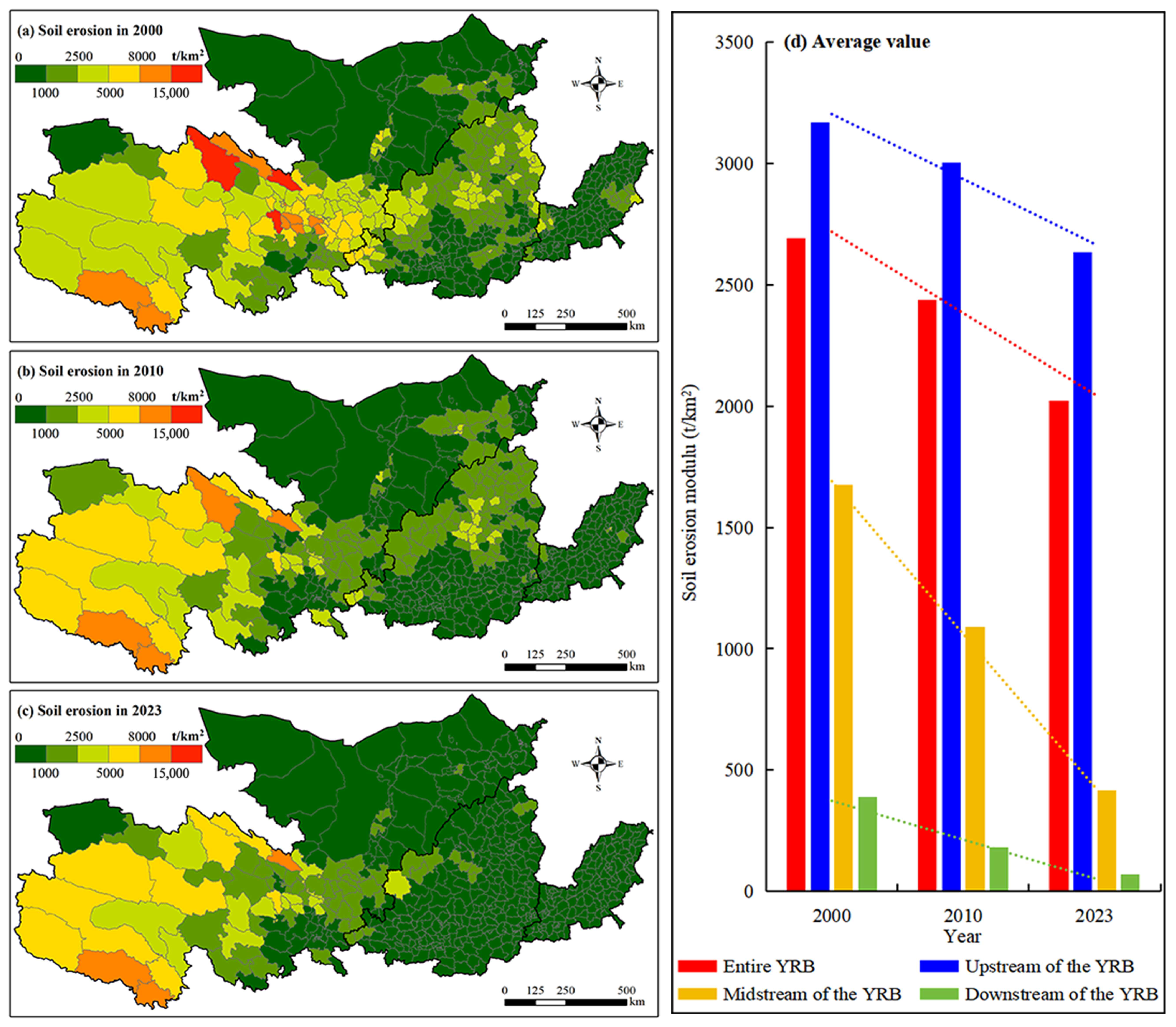
The spatiotemporal characteristics of soil erosion negative service in the YRB are illustrated in Figure 3. Spatially, the distribution pattern of soil erosion negative service remained relatively consistent from 2000 to 2023. It consistently exhibited a pattern of higher values in the west and lower values in the east, showing a sequential decrease from upstream to midstream to downstream. Temporally, soil erosion negative service across the entire YRB displayed a continuous downward trend during the study period. The soil erosion negative service values for 2000, 2010, and 2023 were 2690.42 t/km2, 2437.34 t/km2, and 2020.86 t/km2, respectively. The overall change rate is −24.89%, with an average annual decrease of 29.11 t/(km2·yr). Soil erosion negative service in the upstream, midstream, and downstream of the YRB all showed decreasing trends over time. For the upstream, the modulus values in 2000, 2010, and 2023 were 3168.69 t/km2, 3003.28 t/km2, and 2633.33 t/km2, respectively. This corresponds to a change rate of −16.90% and a reduction rate of 23.28 t/(km2·yr). In the midstream, the modulus values were 1674.56 t/km2, 1091.70 t/km2, and 415.32 t/km2, respectively. This corresponds to a change rate of −75.20% and a reduction rate of 54.75 t/(km2·yr). For the downstream, the modulus values were 389.28 t/km2, 183.43 t/km2, and 69.55 t/km2, respectively, representing a change rate of −82.13% and decreasing at an average annual rate of 13.90 t/(km2·yr). Overall, the most pronounced improvement in soil erosion negative service occurred in the midstream of the YRB.

3.1.2. Carbon Sequestration

The spatiotemporal characteristics of carbon sequestration in the YRB are illustrated in Figure 4. Spatially, carbon sequestration exhibited similar distribution patterns throughout the study period. It generally characterized by higher values in the south and east and lower values in the north and west, with the highest values in the midstream followed by the downstream and upstream. From 2000 to 2023, carbon sequestration amounts across the entire YRB and its upstream, midstream, and downstream individually displayed a consistent increasing trend year by year. Specifically, the average carbon sequestration amounts for the entire YRB in 2000, 2010, and 2023 were 485.01 t/km2, 651.96 t/km2, and 743.51 t/km2, respectively. It represented an increase of 53.30% at an average annual rate of 11.24 t/(km2·yr). In the upstream, the amounts were 329.36 t/km2, 418.79 t/km2, and 440.61 t/km2, respectively. This corresponds to an increase of 33.78% at an average annual rate of 4.84 t/(km2·yr). In the midstream, the amounts were 921.02 t/km2, 1375.76 t/km2, and 1694.88 t/km2, respectively. This corresponds to a change rate of 84.02% and an average annual rate of 33.65 t/(km2·yr). In the downstream, the amounts were 885.02 t/km2, 1023.07 t/km2, and 1189.79 t/km2, respectively, indicating an increase of 34.44% at an average annual rate of 13.25 t/(km2·yr). Overall, the most pronounced improvement in carbon sequestration capacity occurred in the midstream of the YRB.

3.1.3. Water Yield

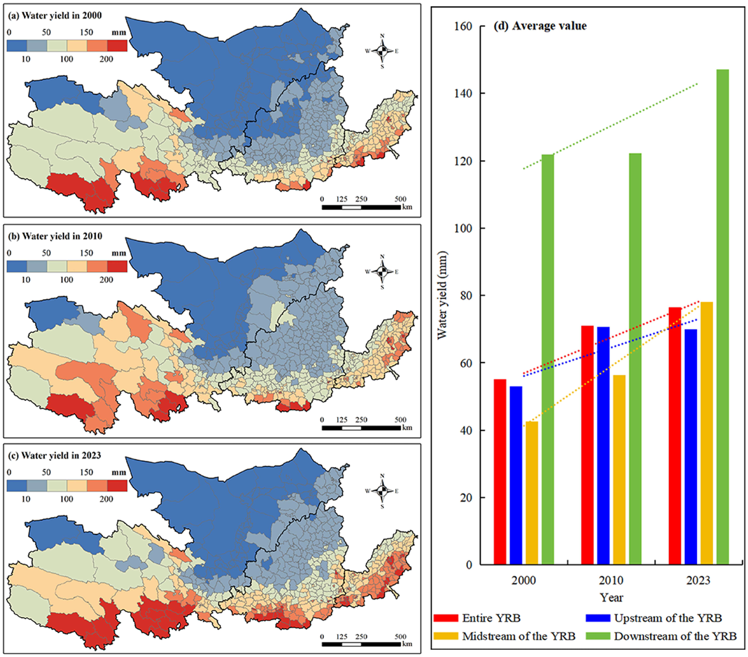
The spatiotemporal characteristics of water yield in the YRB are illustrated in Figure 5. From 2000 to 2023, the spatial distribution of water yield consistently exhibited a pattern of decreasing from south to north. Significant spatial variation existed from the upstream to downstream, with the downstream having the highest water yield. Temporally, water yield across the entire YRB, as well as in its upstream, midstream, and downstream individually, showed an increase compared to the initial period. Specifically, the average water yield for the entire YRB in 2000, 2010, and 2023 was 55.21 mm, 71.01 mm, and 76.45 mm, respectively. It represented an increase of 38.47% at a rate of 0.92 mm/yr. In the upstream, the amounts were 53.01 mm, 70.72 mm, and 69.95 mm, respectively. It showed an increase of 31.96% at a rate of 0.74 mm/yr. In the midstream, the amounts were 42.67 mm, 56.32 mm, and 78.09 mm, respectively. This corresponds to a significant increase of 83.01% at a rate of 1.54 mm/yr. In the downstream, the amounts were 121.82 mm, 122.16 mm, and 147.21 mm, respectively. This is equivalent to an increase of 20.84% at a rate of 1.10 mm/yr. Overall, the most significant increase in water yield capacity occurred in the midstream of the YRB.

3.2. Tradeoff and Synergy Relationships Between ES Pairs

3.2.1. Overall Tradeoff/Synergy Among ESs

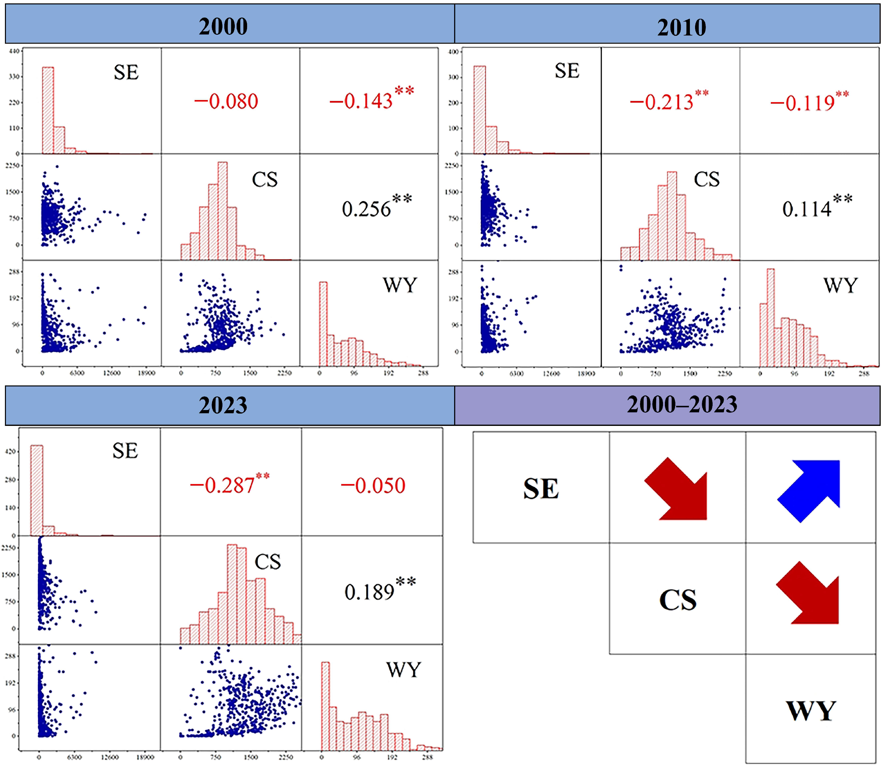
We found that tradeoff relationships were exhibited between soil erosion negative service and carbon sequestration and between soil erosion negative service and water yield. In contrast, a synergistic relationship was observed between carbon sequestration and water yield (Figure 6). That is, as soil erosion decreased, carbon sequestration and water yield increased synergistically. Further examining the temporal change characteristics, we found that the relationships between soil erosion negative service and carbon sequestration as well as between carbon sequestration and water yield showed characteristics shifting toward tradeoff direction. Conversely, the relationship between soil erosion negative service and water yield exhibited a trend shifting toward a synergistic direction.

3.2.2. Spatial Tradeoff /Synergy Among ESs

The GWR results indicated spatial heterogeneity in both tradeoffs and synergies among soil erosion negative service, carbon sequestration, and water yield across the YRB, with marked differences in the spatial distribution patterns for each ES pair (Figure 7a). Statistical analysis (Figure 7b) revealed that the proportion of spatially synergistic areas decreased over time for the pairs of soil erosion negative service–carbon sequestration, soil erosion negative service–water yield, and carbon sequestration–water yield. However, the synergistic areas still predominated over tradeoff areas throughout the study period. This dominance was particularly pronounced for the pair of carbon sequestration-water yield, where synergistic areas exceeded 78% of the basin annually. Taking 2023 as an example, spatial synergy between soil erosion negative service and carbon sequestration primarily occurred in the downstream, the Jizi Bay region, and the westernmost parts (with stronger synergy in the westernmost). Spatial tradeoffs clustered in the central YRB, including the eastern part of the upstream and the midstream of the YRB, exhibiting weaker intensity. For soil erosion negative service and water yield, synergy was mainly found in the northwestern and eastern parts, with a stronger synergy effect in the northwestern region of the YRB. Conversely, tradeoffs were concentrated in the Loess Plateau region with weaker intensity. The spatial synergy effect between carbon sequestration and water yield covered extensive areas across the midstream and upstream, with a stronger synergy effect in the northernmost part of the YRB. Tradeoffs, however, were mainly distributed in the eastern midstream and downstream, also showing weaker intensity.

3.3. Driving Forces of ES Tradeoff/Synergy

3.3.1. Parameter Discretization Results

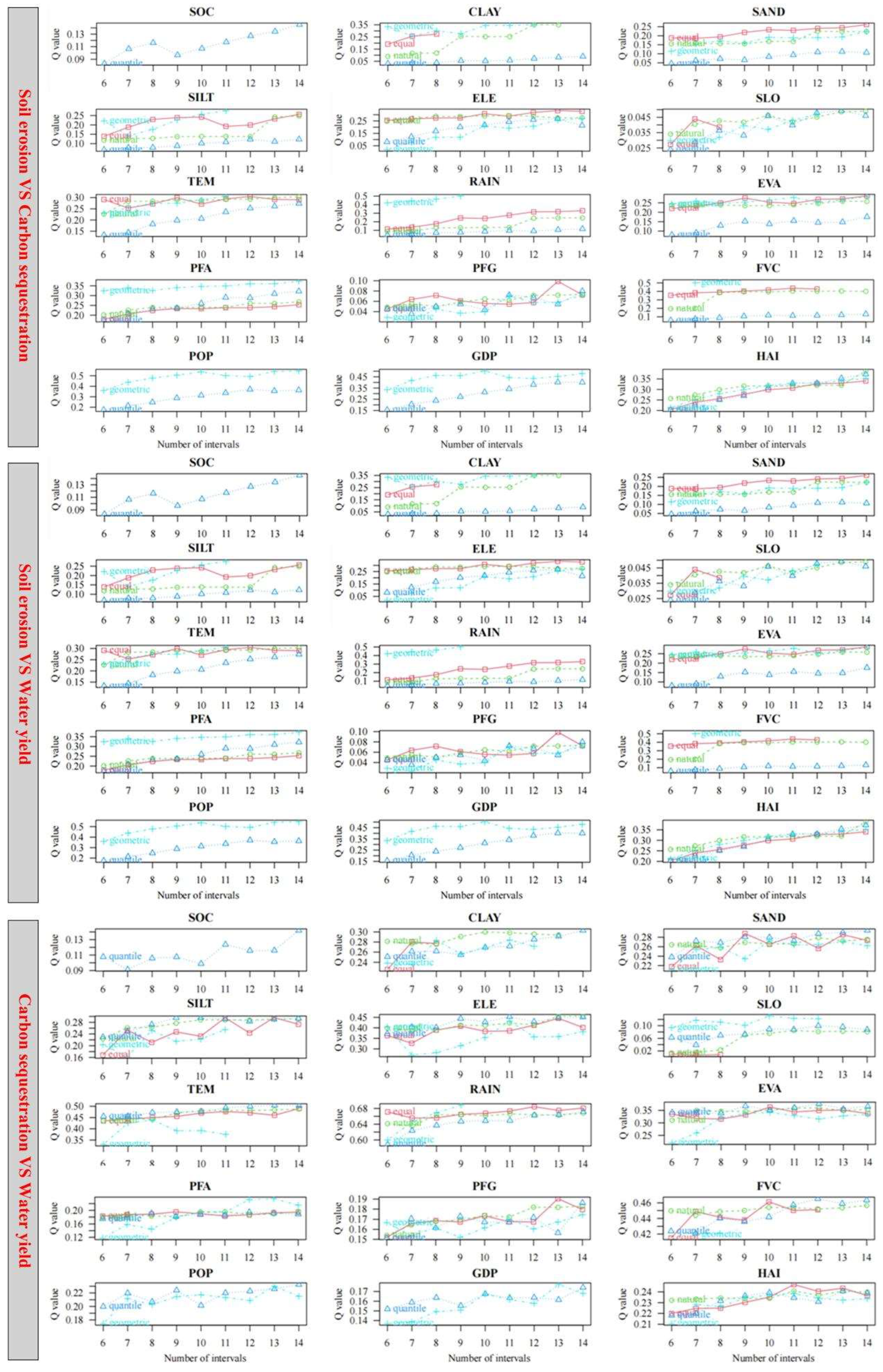
The parameter discretization results are shown in Figure 8. It can be observed that the Q values for each factor differed significantly across classification methods and numbers of intervals. For different factors corresponding to different ES pairs, we selected the parameter combination (classification method and number of interval) that yielded the highest Q value as the optimal discretization approach. This selected parameter combination effectively captured the heterogeneity of the underlying spatial stratification, particularly focusing on the importance of key continuous variables.

3.3.2. Driving Forces Results

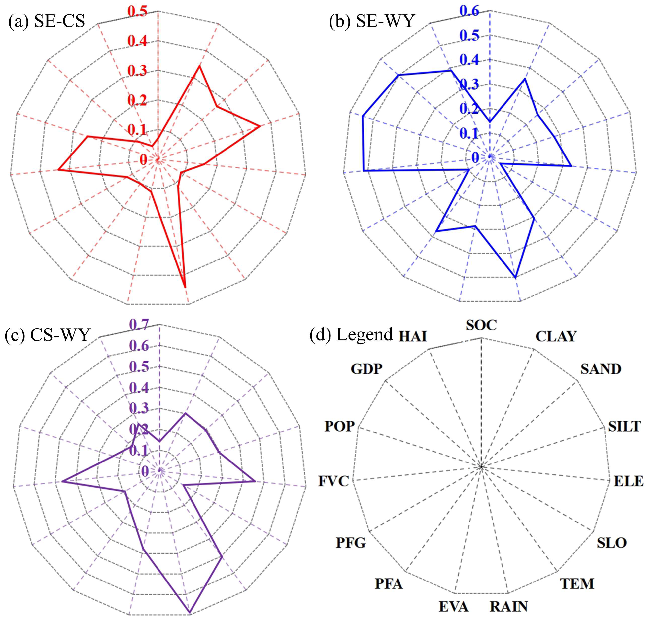
We investigated the driving mechanisms behind the changes in tradeoff/synergy intensity among soil erosion negative service, carbon sequestration, and water yield in the YRB (Figure 9). The results indicated significant differences in the degree of influence exerted by various factors on the interactions between different ES pairs. Specifically, rainfall (Q = 0.441) was the dominant factor influencing the tradeoff/synergy relationship between soil erosion negative service and carbon sequestration, followed by silt content (Q = 0.361), clay content (Q = 0.344), and fractional vegetation cover (Q = 0.338). Meanwhile, rainfall (Q = 0.689) also exhibited the most prominent explanatory power for the interactions between carbon sequestration and water yield, followed by temperature (Q = 0.505), fractional vegetation cover (Q = 0.465), and elevation (Q = 0.456). For the tradeoff/synergy relationship between soil erosion negative service and water yield, population density had the strongest influence (Q = 0.546), followed by fractional vegetation cover (Q = 0.518), GDP density (Q = 0.502), and rainfall (Q = 0.501). Overall, the tradeoff/synergy relationship between soil erosion negative service and carbon sequestration was primarily driven by rainfall, soil properties, and vegetation cover. The relationship between carbon sequestration and water yield was mainly influenced by climate, vegetation cover, and elevation. The relationship between soil erosion negative service and water yield was predominantly affected by socioeconomic conditions, vegetation cover, and rainfall. Clearly, both rainfall and fractional vegetation cover have significant influences in explaining the tradeoff/synergy dynamics across all ES pairs.

4. Discussion

4.1. The Development of ESs After the GFGP

The GFGP, a landmark ecological restoration policy in China, has profoundly reshaped the ecological trajectory of the YRB since its full implementation in 2000. Our analysis reveals an overall improvement trend in soil conservation capacity, carbon sequestration capacity, and water yield capacity across the basin from 2000 to 2023, albeit with significant regional variations.
Soil erosion negative service decreased by 24.89%, with the most striking reduction observed in the midstream (−75.20%). This is closely linked to the regional status as a core implementation zone of the GFGP [47], which has also received strong support by the re-search of Wu et al. [48] on the Loess Plateau region. The conversion of large areas of slop-ing cropland to forests and grasslands enhanced fractional vegetation cover, directly mit-igating raindrop splash and runoff scouring. Coupled with supporting soil and water conservation programs like terraces and fish-scale pits [49,50], this led to an average an-nual erosion modulus reduction of 54.75 t/km2 in the midstream, particularly within the Loess Plateau. Although soil erosion negative service in the upstream decreased by 16.90%, the absolute value (2633.33 t/km2) remained significantly higher than in the mid-stream (415.32 t/km2) and downstream (69.55 t/km2). This disparity may stem from chal-lenges in vegetation recovery due to harsh high-cold arid conditions, severe climate, and unresolved grazing pressure [51] and also highlights the rigid constraints imposed by the natural background on the program’s effectiveness in the upstream. The increase in car-bon sequestration capacity was particularly remarkable, with a basin-wide rise of 53.30%. The midstream emerged as the primary contributor with an 84.02% growth rate. This finding is also similar to the results of Fang et al. [52], who studied the YRB, and found that the growth of NPP is mainly concentrated in the Shaanxi region. This may be related to the synergistic increase in biomass accumulation and soil organic carbon pools driven by the expansion of planted forests and grasslands [53,54]. Studies indicate that convert-ing cropland to trees, shrubs, and grassland significantly enhances soil organic carbon sequestration by 88.20%, 55.15%, and 43.18%, respectively, compared to farmland [55]. Notably, the spatial distribution of carbon sequestration exhibited a pattern of “higher in the south and east, lower in the north and west,” reflecting, to some extent, the controlling role of hydrothermal conditions on vegetation productivity [56]. Despite a lower growth rate (34.44%) in the downstream, the high baseline value (1189.79 t/km2) made its carbon sequestration contribution per unit area still not negligible. Water yield dynamics pre-sented a more complex mechanism. Basin-wide water yield increased by 38.47%, led by the midstream with an 83.01% surge. This phenomenon appears paradoxical to the ex-pectation that the increase in evapotranspiration due to vegetation recovery may lead to a reduction in water yield. This discrepancy is likely due to increased regional rainfall over the past two decades, which offset the negative impact of enhanced evapotranspiration caused by vegetation restoration [57,58], also aligning with findings from Wang and Xu [59] and Huang et al. [60]. In contrast, the water yield increase in the upstream (31.96%) was primarily driven by precipitation fluctuations. The downstream, however, saw a rela-tively limited increase (20.84%), possibly constrained by increased water abstraction for agricultural irrigation.
Crucially, the midstream emerged as a hotspot for ecosystem improvement, highlighting the effectiveness of the GFGP in this ecologically fragile and program-intensive region. This area simultaneously achieved a sharp reduction in soil erosion, a surge in carbon sequestration, and a significant increase in water yield, forming a triple-synergy pattern of “erosion reduction—carbon sequestration increase—water yield increase”. This demonstrates that the GFGP successfully initiated a positive ecological feedback loop in this critical zone and challenges the traditional tradeoff expectation that “erosion control inevitably suppresses water yield” [61,62].

4.2. The Influencing Mechanism of Tradeoff/Synergy Among Pairwise ESs

Correlation analysis revealed the dynamic interactions among ESs. The predominant synergy between carbon sequestration and water yield aligns with the expected outcomes of vegetation restoration. The enhanced canopy cover and root systems concurrently boost carbon uptake and regulate water fluxes, improving infiltration and baseflow [62,63]. This help to achieve synergistic gains in both carbon sequestration and water yield. Simulta-neously, the observed tradeoffs between soil erosion negative service and carbon seques-tration and between soil erosion negative service and water yield are encouraging. This signifies that the increases in carbon sequestration and water yield under vegetation res-toration also achieve the most fundamental objective of project implementation (i.e., re-ducing soil erosion), which has also been supported by the studies of Wu et al. [48] and An et al. [64]. However, GWR results strongly demonstrate that these interactions exhibit spatial location dependency. That is to say, the tradeoffs between carbon sequestration and water yield or the synergy between soil erosion negative service and carbon seques-tration as well as soil erosion negative service and water yield in some spatial regions are not what we wish to see. It was this spatial heterogeneity that motivated us to fur-ther employ the OPGD to pinpoint the dominant forces driving these spatial tradeoffs/synergies. This further helps to reveal the unique mechanisms of interaction among different ESs with the hope of providing a basis for conflict-mitigation management strategies.
We found that the interaction between soil erosion negative service and carbon se-questration is predominantly governed by natural factors. Rainfall is the most critical, serving both as the primary energy source for erosion processes and as a key regulator of vegetation productivity by controlling water availability [56]. Soil texture significantly in-fluences both soil erodibility and carbon stabilization capacity. Fractional vegetation cover directly mediates these processes by stabilizing the surface matrix and providing organic inputs [53]. Collectively, these three factors underscore the fundamental efficacy of climate forcing, pedogenic properties, and vegetation structural dynamics in shaping the interac-tion patterns between soil erosion negative service and carbon sequestration. For the in-teraction between carbon sequestration and water yield, climatic drivers again exerted strong control. Rainfall and temperature are key explanatory variables, governing water availability and photosynthetic activity [54]. Fractional vegetation cover acts as a bio-physical linchpin, directly coupling carbon fixation with hydrological partitioning through canopy interception and root-zone processes [10,65]. Elevation integrates gradi-ents of temperature, moisture, and vegetation type [66], thereby influencing the character-istics of their interaction. This hierarchy also emphasizes that the synergistic effect of cli-mate (hydrothermal conditions) and vegetation cover is the core mechanism controlling the “carbon–water nexus” in the YRB. Conversely, socioeconomic drivers predominated in the interaction between soil erosion negative service and water yield. This distinct an-thropogenic signature highlights the profound and growing human influence on ero-sion-water yield dynamics, particularly in this rapidly developing basin. Population den-sity exerted the strongest control. This may reflect the compound pressures from land-use intensification (e.g., expansion of irrigated agriculture), the proliferation of impervious surfaces due to infrastructure development, and water abstraction that reconfigures runoff generation and sediment source–sink dynamics [13,67]. Fractional vegetation cover retains a crucial role by mediating the impact of land cover on infiltration capacity [62]. GDP den-sity signifies the capacity of economic activity to influence land management and reshape hydrological infrastructure (e.g., silt arrester, reservoirs, canals). Rainfall provides the fundamental hydrological context, thereby influencing their relationship.
The cross-cutting significance of rainfall and fractional vegetation cover across all three ES pairs represents a key finding. Rainfall establishes the fundamental hydrological forcing governing erosion energy, carbon assimilation, and runoff generation, while fractional vegetation cover represents the primary lever through which human intervention (e.g., GFGP-driven afforestation) modulates biophysical processes. Such a finding underscores the pervasive influence of climate and vegetation restoration strategies on ESs interactions within the YRB. Consequently, it necessitates the development of climate-adaptive vegetation restoration strategies—for instance, prioritizing drought-tolerant species in arid regions and regulating stand density in humid areas—to balance multiple ES objectives.

4.3. Limitations and Prospects

This study, however, like other similar studies, has some limitations that future work can further address. First, it is foreseeable that there are errors and uncertainties in the as-sessment of ESs. On the one hand, uncertainty comes from the model itself. On the other hand, the data input to the model would also affect the simulation results. Secondly, alt-hough the selection of the county scale as the basic unit is convenient for decision making to enhance the convenience of governance application, we must also admit that the con-clusions drawn at a single scale may not be applicable to other scales [13,16,34]. Future research should consider exploring at multiple scales, such as different grid sizes, water-shed, township, etc., may provide a richer theoretical basis for managers working at a range of scales. In addition, our analysis focused specifically on the latest driving mecha-nisms of ESs interactions in the YRB. Future research could incorporate a temporal scale to examine the dynamic influences between ES interactions and their driving factors over time. Meanwhile, a deeper understanding of the interactions among ESs is needed to clar-ify how biophysical processes affect ES functions and ES spatiotemporally in the context of climate change versus anthropic interventions.

5. Conclusions

We found that the three ESs in the YRB exhibited spatiotemporal heterogeneity in their changes. Soil erosion negative service decreased at an average annual rate of 29.11 t/km2 from 2000 to 2023, showing a general spatial pattern of higher values in the west and lower values in the east. Carbon sequestration increased at an average annual rate of 11.24 t/km2, exhibiting a spatial pattern of higher values in the south and east and lower values in the north and west. Water yield increased at an average annual rate of 0.92 mm, displaying a spatial pattern decreasing from south to north. The midstream of the YRB emerged as the core area of ES improvement. Overall tradeoff relationships existed between soil erosion negative service and carbon sequestration and between soil erosion negative service and water yield, while an overall synergistic relationship existed between carbon sequestration and water yield. The proportion of areas showing synergy among the three ES pairs decreased over time but remained higher than the proportion of areas showing tradeoff during the study period. This was especially evident in the relationship between carbon sequestration and water yield, where synergy consistently accounted for over 78% of the basin. The spatial tradeoff effects between soil erosion negative service and carbon sequestration and between soil erosion negative service and water yield were primarily clustered in the Loess Plateau region, whereas the spatial synergistic effect between carbon sequestration and water yield showed contiguous distribution in the midstream and upstream of the YRB. The tradeoff/synergy relationships of different ES pairs were influenced by distinct driving factors. Rainfall, soil properties, and fractional vegetation cover were important drivers for the relationship between soil erosion negative service and carbon sequestration. Rainfall, temperature, fractional vegetation cover, and elevation significantly drove the interactions between carbon sequestration and water yield. Population density, fractional vegetation cover, GDP density, and rainfall were the main influencing factors for the interactions between soil erosion negative service and water yield. Our findings provide significant theoretical foundations for the YRB and similar regions, offering a scientific basis for formulating ecological conservation policies and resource management measures.

Author Contributions

Conceptualization, M.Y. and L.C.; data curation, M.Y.; methodology, M.Y., M.W., L.C. and H.Z.; validation, H.N. and J.L.; investigation, M.Y., M.W., H.N. and J.L.; writing—original draft preparation, M.Y., M.W. and L.C.; writing—review and editing, M.Y., L.C., H.Z., H.N. and J.L.; project administration, L.C.; funding acquisition, M.Y. All authors have read and agreed to the published version of the manuscript.

Funding

This research was funded by the National Natural Science Foundation of China (42401384), the Humanities and Social Sciences Foundation of Ministry of Education of China (24YJCZH376), and the Key Scientific Research Projects of Colleges and Universities in Henan Province (25A170008).

Data Availability Statement

The data that support the findings of this study are available from the corresponding author upon reasonable request.

Acknowledgments

We appreciate the four anonymous reviewers and their valuable comments. Also, we thank Editors for the editing and comments.

Conflicts of Interest

The authors declare no conflicts of interest.

References

  1. Ouyang, Z.; Zheng, H.; Xiao, Y.; Polasky, S.; Liu, J.; Xu, W.; Wang, Q.; Zhang, L.; Xiao, Y.; Rao, E.; et al. Improvements in ecosystem services from investments in natural capital. Science 2016, 352, 1455–1459. [Google Scholar] [CrossRef]
  2. Reid, W.V.; Mooney, H.A.; Cropper, A.; Capistrano, D. Millennium Ecosystem Assessment. Ecosystems and Human Well-Being; Island Press: Washington, DC, USA, 2005. [Google Scholar]
  3. Bai, Y.; Wong, C.P.; Jiang, B.; Hughes, A.C.; Wang, M.; Wang, Q. Developing China’s ecological redline policy using ecosystem services assessments for land use planning. Nat. Commun. 2018, 9, 3034. [Google Scholar] [CrossRef]
  4. Schröter, M.; Crouzat, E.; Hölting, L.; Massenberg, J.; Rode, J.; Hanisch, M.; Kabisch, N.; Palliwoda, J.; Priess, J.A.; Seppelt, R.; et al. Assumptions in ecosystem service assessments: Increasing transparency for conservation. Ambio 2021, 50, 289–300. [Google Scholar] [CrossRef]
  5. IPBES. Summary for Policymakers of the Global Assessment Report on Biodiversity and Ecosystem Services of the Intergovernmental Science-Policy Platform on Biodiversity and Ecosystem Services. 2019. Available online: https://www.ipbes.net/system/tdf/spm_global_unedited_advance.pdf?file=1&type=node&id=35245 (accessed on 12 March 2025).
  6. Su, B.; Liu, M. How to manage the ecosystem services effectively and fairly? J. Clean. Prod. 2024, 458, 142477. [Google Scholar] [CrossRef]
  7. Simeon, M.; Wana, D. Synergies and trade-offs among key ecosystem services in Maze National Park and its environs, southwestern Ethiopia. Glob. Ecol. Conserv. 2025, 57, e03398. [Google Scholar] [CrossRef]
  8. Huang, L.; Du, Y.; Tang, Y. Ecosystem service trade-offs and synergies and their drivers in severely affected areas of the Wenchuan earthquake, China. Land Degrad. Dev. 2024, 35, 3881–3896. [Google Scholar] [CrossRef]
  9. Schwantes, A.M.; Firkowski, C.R.; Gonzalez, A.; Fortin, M.J. Revealing driver-mediated indirect interactions between ecosystem services using Bayesian Belief Networks. Ecosyst. Serv. 2025, 73, 101717. [Google Scholar] [CrossRef]
  10. Feng, Z.; Jin, X.; Chen, T.; Wu, J. Understanding trade-offs and synergies of ecosystem services to support the decision-making in the Beijing–Tianjin–Hebei region. Land Use Policy 2021, 106, 105446. [Google Scholar] [CrossRef]
  11. Chen, S.; Liu, X.; Yang, L.; Zhu, Z. Variations in Ecosystem Service Value and Its Driving Factors in the Nanjing Metropolitan Area of China. Forests 2023, 14, 113. [Google Scholar] [CrossRef]
  12. Rodriguez, J.P.; Beard, T.D., Jr.; Bennett, E.M.; Cumming, G.S.; Cork, S.J.; Agard, J.; Dobson, A.P.; Peterson, G.D. Trade-offs across space, time, and ecosystem services. Ecol. Soc. 2006, 11, 28. [Google Scholar] [CrossRef]
  13. Yang, M.; Gao, X.; Zhao, X.; Wu, P. Scale effect and spatially explicit drivers of interactions between ecosystem services—A case study from the Loess Plateau. Sci. Total Eviron. 2021, 785, 147389. [Google Scholar] [CrossRef]
  14. Karimi, J.D.; Corstanje, R.; Harris, J.A. Bundling ecosystem services at a high resolution in the UK: Trade-offs and synergies in urban landscapes. Landsc. Ecol. 2021, 36, 1817–1835. [Google Scholar] [CrossRef]
  15. Zhang, J.; Wang, M.; Liu, K.; Chen, S.; Zhao, Z. Social-ecological system sustainability in China from the perspective of supply-demand balance for ecosystem services. J. Clean. Prod. 2025, 497, 145039. [Google Scholar] [CrossRef]
  16. Xia, H.; Yuan, S.; Prishchepov, A.V. Spatial-temporal heterogeneity of ecosystem service interactions and their social-ecological drivers: Implications for spatial planning and management. Resour. Conserv. Recycl. 2023, 189, 106767. [Google Scholar] [CrossRef]
  17. Hohlenwerger, C.; Spake, R.; Tambosi, L.R.; Aristizábal, N.; González-Chaves, A.; Librán-Embid, F.; Saturni, F.; Eigenbrod, F.; Metzger, J.P. Coffee pollination and pest control are affected by edge diversity at local scales but multiscalar approaches and disservices can not be ignored. Landscape Ecol. 2024, 39, 75. [Google Scholar] [CrossRef]
  18. Qu, Q.; Zhang, K.; Niu, J.; Xiao, C.; Sun, Y. Spatial-Temporal Differentiation of Ecosystem Service Trade-Offs and Synergies in the Taihang Mountains, China. Land 2025, 14, 513. [Google Scholar] [CrossRef]
  19. Umwali, E.D.; Chen, X.; Ma, X.; Guo, Z.; Mbigi, D.; Zhang, Z.; Umugwaneza, A.; Gasirabo, A.; Umuhoza, J. Integrated SSP-RCP Scenarios for Modeling the Impacts of Climate Change and Land Use on Ecosystem Services in East Africa. Ecol. Model. 2025, 504, 111092. [Google Scholar] [CrossRef]
  20. Zhang, Z.; Shen, Z.; Liu, L.; Zhang, Y.; Yu, C.; Cui, L.; Gao, Y. Integrating ecosystem services conservation into the optimization of urban planning policies in eco-fragile areas: A scenario-based case study. Cities 2023, 134, 104200. [Google Scholar] [CrossRef]
  21. Lovric, M.; Torralba, M.; Orsi, F.; Pettenella, D.; Mann, C.; Geneletti, D.; Plieninger, T.; Primmer, E.; Hernandez-Morcillo, M.; Thorsen, B.J.; et al. Mind the income gap: Income from wood production exceed income from providing diverse ecosystem services from Europe’s forests. Ecosyst. Serv. 2025, 71, 101689. [Google Scholar] [CrossRef]
  22. Rong, Y.; Zheng, L.; Zhao, Y. Balancing ecosystem services supply-flow-demand for watershed ecological security: A case study of the Hai River Basin, China. Front. Ecol. Evol. 2025, 13, 1587167. [Google Scholar] [CrossRef]
  23. Hu, Y.; Xu, X.; Huang, X.; Li, Y.; Cao, J.; Yan, Y.; Hu, X.; Wu, S. Urban Spatial Management and Planning Based on the Interactions Between Ecosystem Services: A Case Study of the Beijing-Tianjin-Hebei Urban Agglomeration. Remote Sens. 2025, 17, 1258. [Google Scholar] [CrossRef]
  24. Hu, X.; Wang, H.; Fang, Q.; Chang, C.; Li, A.; Wang, H. Integrating ecosystem services trade-off, drivers and zoning into watershed water environment management in Nansihu Lake Basin, China. Ecol. Indic. 2024, 167, 112642. [Google Scholar] [CrossRef]
  25. Ma, X.; Xu, Z.; Zuo, D. Investigating on Trade-offs and Synergies of Ecosystem Services and their Driving Mechanisms Under Different Land Use Scenarios. Water Resour. Manag. 2025, 1–23. [Google Scholar] [CrossRef]
  26. Zhang, H.; Wang, L.; Jiang, S.; Li, K.; Xin, X.; Huang, X.; Chen, J.; Zhou, L.; Li, Z. Impacts of rice-crayfish co-culture on ecosystem service trade-offs/ synergies in agricultural watersheds: A case exploration in Sihu Lake Basin, China. Agr. Water Manag. 2025, 310, 109389. [Google Scholar] [CrossRef]
  27. Brück, M.; Fischer, J.; Law, E.A.; Schultner, J.; Abson, D.J. Drivers of ecosystem service specialization in a smallholder agricultural landscape of the Global South: A case study in Ethiopia. Ecol. Soc. 2023, 28, 1. [Google Scholar] [CrossRef]
  28. Li, Y.; Geng, H. Spatiotemporal trends in ecosystem carbon stock evolution and quantitative attribution in a karst watershed in southwest China. Ecol. Indic. 2023, 153, 110429. [Google Scholar] [CrossRef]
  29. Liu, L.; Wang, J.; Li, J.; He, S.; Lan, Y.; Liu, F. Evaluation of Ecosystem Service Capacity Using the Integrated Ecosystem Services Index at Optimal Scale in Central Yunnan, China. Ecol. Evol. 2025, 15, e71222. [Google Scholar] [CrossRef] [PubMed]
  30. Yang, M.; Gao, X.; Siddique, K.H.M.; Wu, P.; Zhao, X. Spatiotemporal exploration of ecosystem service, urbanization, and their interactive coercing relationship in the Yellow River Basin over the past 40 years. Sci. Total Eviron. 2023, 858, 159757. [Google Scholar] [CrossRef] [PubMed]
  31. Fu, B.; Wang, S.; Shen, Y.; Cheng, C.; Li, Y.; Feng, X.; Liu, Y. Mechanisms of Human-natural System Coupling and Optimization of the Yellow River Basin. Bull. Natl. Nat. Sci. Found. China 2021, 35, 504–509. (In Chinese) [Google Scholar]
  32. Song, S.; Wen, H.; Wang, S.; Wu, X.; Cumming, G.S.; Fu, B. Quantifying the effects of institutional shifts on water governance in the Yellow River Basin: A social-ecological system perspective. J. Hydrol. 2024, 629, 130638. [Google Scholar] [CrossRef]
  33. Wang, Y.; Chen, Y.; Wang, H.; Lv, Y.; Hao, Y.; Cui, X.; Wang, Y.; Hu, R.; Xue, K.; Fu, B. Ecosystem Change and Its Ecohydrological Effect in the Yellow River Basin. Bull. Natl. Nat. Sci. Found. China 2021, 35, 520–528. (In Chinese) [Google Scholar]
  34. Ji, Q.; Feng, X.; Sun, S.; Zhang, J.; Li, S.; Fu, B. Cross-scale coupling of ecosystem service flows and socio-ecological interactions in the Yellow River Basin. J. Environ. Manag. 2024, 367, 122071. [Google Scholar] [CrossRef]
  35. Zhou, Z.; Sun, X.; Zhang, X.; Wang, Y. Estimation and influencing factors of agricultural water efficiency in the Yellow River basin, China. J. Environ. Manag. 2022, 322, 116073. [Google Scholar] [CrossRef]
  36. Wischmeier, W.H.; Smith, D.D. Rainfall energy and its relationship to soil loss. Trans. Am. Geophys. Union 1958, 39, 285–291. [Google Scholar] [CrossRef]
  37. Williams, J.R.; Jones, C.A.; Kiniry, J.R.; Spanel, D.A. The EPIC crop growth-model. Trans. ASAE 1989, 32, 497–511. [Google Scholar] [CrossRef]
  38. Liu, B.; Nearing, M.A.; Risse, L.M. Slope Gradient Effects on Soil Loss for Steep Slopes. Trans. ASAE 1994, 37, 1835–1840. [Google Scholar] [CrossRef]
  39. Cai, C.; Ding, S.; Shi, Z.; Huang, L.; Zhang, G. Study of applying USLE and geographical information system IDRISI to predict soil erosion in small watershed. J. Soil Water Conserv. 2000, 14, 19–24. (In Chinese) [Google Scholar]
  40. Huang, S.; Li, J.; Zhang, X.; Deng, L.; Zhang, J. Analysis of spatial and temporal changes in soil erosion in Henan Province over the last ten years. J. Agr. Resour. Environ. 2021, 38, 232–240. (In Chinese) [Google Scholar]
  41. Xiao, Y.; Guo, B.; Lu, Y.; Zhang, R.; Zhang, D.; Zhen, X.; Chen, S.; Wu, H.; Wei, C.; Yang, L.; et al. Spatial–temporal evolution patterns of soil erosion in the Yellow River Basin from 1990 to 2015: Impacts of natural factors and land use change. Geomat. Nat. Haz. Risk 2021, 12, 103–122. [Google Scholar] [CrossRef]
  42. Yin, Z.; Chang, J. Analysis of soil erosion and its driving factors in the Yellow River Basin from 2000 to 2020. J. Xi’an Univ. Technol. 2023, 39, 360–368. [Google Scholar]
  43. Zhao, M.; Peng, J.; Liu, Y.; Li, T.; Wang, Y. Mapping Watershed-Level Ecosystem Service Bundles in the Pearl River Delta, China. Eco. Econ. 2018, 152, 106–117. [Google Scholar] [CrossRef]
  44. Liu, C.; Liu, J.; Zhang, L.; Shrestha, U.B.; Luo, D.; Wei, Y.; Wang, J. Assessing Climate and Land Use Change Impacts on Ecosystem Services in the Upper Minjiang River Basin. Remote Sens. 2025, 17, 1884. [Google Scholar] [CrossRef]
  45. Yang, J.; Xie, B.; Zhang, D. Spatio-temporal variation of water yield and its response to precipitation and land use change in the Yellow River Basin based on InVEST model. Chin. J. Appl. Ecol. 2020, 31, 2731–2739. (In Chinese) [Google Scholar]
  46. Mashizi, A.K.; Sharafatmandrad, M. Dry forests conservation: A comprehensive approach linking ecosystem services to ecological drivers and sustainable management. Glob. Ecol. Conserv. 2023, 47, e02652. [Google Scholar] [CrossRef]
  47. He, Z.; Geng, G.; Zheng, R. Variation Characteristics and Its Driving Forces of Fractional Vegetation Cover in the Shaanxi Section of the Yellow River Basin Under the Background of the Grain for Green Program. Environ. Sci. 2025. (In Chinese) [Google Scholar] [CrossRef]
  48. Wu, X.; Wang, S.; Fu, B.; Feng, X.; Chen, Y. Socio-ecological changes on the Loess Plateau of China after Grain to Green Program. Sci. Total Eviron. 2019, 678, 565–573. [Google Scholar] [CrossRef] [PubMed]
  49. Sun, C.; Hou, H.; Chen, W. Effects of vegetation cover and slope on soil erosion in the Eastern Chinese Loess Plateau under different rainfall regimes. PeerJ 2021, 9, e11226. [Google Scholar] [CrossRef] [PubMed]
  50. Tian, P.; Tian, X.; Geng, R.; Zhao, G.; Yang, L.; Mu, X.; Gao, P.; Sun, W.; Liu, Y. Response of soil erosion to vegetation restoration and terracing on the Loess Plateau. CATENA 2023, 227, 107103. [Google Scholar] [CrossRef]
  51. Zheng, Z.; Lv, M.; Ma, Z. Climate, Hydrology, and Vegetation Coverage Changes in Source Region of Yellow River and Countermeasures for Challenges. Bull. Chin. Acad. Sci. 2020, 35, 61–72. (In Chinese) [Google Scholar]
  52. Fang, L.; Xu, D.; Wang, L.; Niu, Z.; Zhang, M. The study of ecosystem services and the comparison of trade-off and synergy in Yangtze River Basin and Yellow River Basin. Geogr. Res. 2021, 40, 821–838. (In Chinese) [Google Scholar]
  53. Lu, F.; Hu, H.; Sun, W.; Zhu, J.; Liu, G.; Zhou, W.; Zhang, Q.; Shi, P.; Liu, X.; Wu, X.; et al. Effects of national ecological restoration projects on carbon sequestration in China from 2001 to 2010. Proc. Natl. Acad. Sci. USA 2018, 115, 4039–4044. [Google Scholar] [CrossRef]
  54. Zhang, Y.; Wang, Z.; Lu, X.; Xiao, P.; Zhao, G. Evolution of ecosystem carbon sink and its driving factors in the Loess Plateau. Res. Soil. Water Conserv. 2025, 32, 266–274+284. (In Chinese) [Google Scholar]
  55. Lin, F.; Wang, L.; Wen, Q. Dynamic Responses of Sequestration of Soil Organic Carbon to Vegetation Restoration and the Values of Carbon Sink in the Loess Plateau. Res. Soil. Water Conserv. 2021, 28, 53–58. (In Chinese) [Google Scholar]
  56. Yang, Y.; Yin, J.; Slater, L.J.; Liu, P.; Zhang, L.Q.; Zhang, Y. Global vegetation dynamics under decreased terrestrial water storage: Insights into water stress response. Agr. Forest Meteorol. 2025, 368, 110549. [Google Scholar] [CrossRef]
  57. Li, Y.; Piao, S.; Li, L.Z.; Chen, A.; Wang, X.; Ciais, P.; Huang, L.; Lian, X.; Peng, S.; Zeng, Z.Z.; et al. Divergent hydrological response to large-scale afforestation and vegetation greening in China. Sci. Adv. 2018, 4, eaar4182. [Google Scholar] [CrossRef] [PubMed]
  58. Su, W.; Yang, Y.; Wang, T.; Su, L.; Wang, Y. Variation Characteristics and Influencing Factors of Drought in the Loess Plateau in Recent 20 Years. Sci. Technol. Eng. 2023, 23, 4551–4560. (In Chinese) [Google Scholar]
  59. Wang, P.; Xu, M. Evaluating the inter-annual surplus/deficit dynamic of water retention service in the Yellow River Basin, China. Ecol. Indic. 2022, 145, 109695. [Google Scholar] [CrossRef]
  60. Huang, W.; Wang, P.; He, L.; Liu, B. Improvement of water yield and net primary productivity ecosystem services in the Loess Plateau of China since the “Grain for Green” project. Ecol. Indic. 2023, 154, 110707. [Google Scholar] [CrossRef]
  61. Jiang, C.; Zhang, H.; Zhang, Z. Spatially explicit assessment of ecosystem services in China’s Loess Plateau: Patterns, interactions, drivers, and implications. Glob. Planet Change 2018, 161, 41–52. [Google Scholar] [CrossRef]
  62. Xun, B.; Zheng, Y.; Fan, R.; Hao, R.; Liu, B. Assessment of trade-off/synergy relationships between ecosystem services andidentification of ecological restoration thresholds. Acta Ecol. Sin. 2024, 44, 7431–7444. (In Chinese) [Google Scholar]
  63. Duan, R.; Li, X.; Zhang, Q. Spatio-temporal Variation of Ecosystem Service Trade-offs/Synergies and Ecosystem Service Bundles in Western Jilin. Environ. Sci. 2025. (In Chinese) [Google Scholar] [CrossRef]
  64. An, J.; Yuan, X.; Yang, R.; An, Q.; Su, Q. Effeet of the Grain for Green Program on Ecosystem Services in Northern Shaanxi, China. Environ. Sci. 2025, 46, 2410–2427. (In Chinese) [Google Scholar]
  65. Feng, X.; Fu, B.; Piao, S.; Wang, S.; Ciais, P.; Zeng, Z.; Lü, Y.; Zeng, Y.; Li, Y.; Jiang, X.; et al. Revegetation in China’s Loess Plateau is approaching sustainable water resource limits. Nat. Clim. Change 2016, 6, 1019–1022. [Google Scholar] [CrossRef]
  66. Gomes, L.C.; Bianchi, F.J.J.A.; Cardoso, I.M.; Fernandes, E.I.; Schulte, R.P.O. Land use change drives the spatio-temporal variation of ecosystem services and their interactions along an altitudinal gradient in Brazil. Landsc. Ecol. 2020, 35, 1571–1586. [Google Scholar] [CrossRef]
  67. Jantz, C.A.; Manuel, J.J. Estimating impacts of population growth and land use policy on ecosystem services: A community-level case study in Virginia, USA. Ecosyst. Serv. 2013, 5, 110–123. [Google Scholar] [CrossRef]
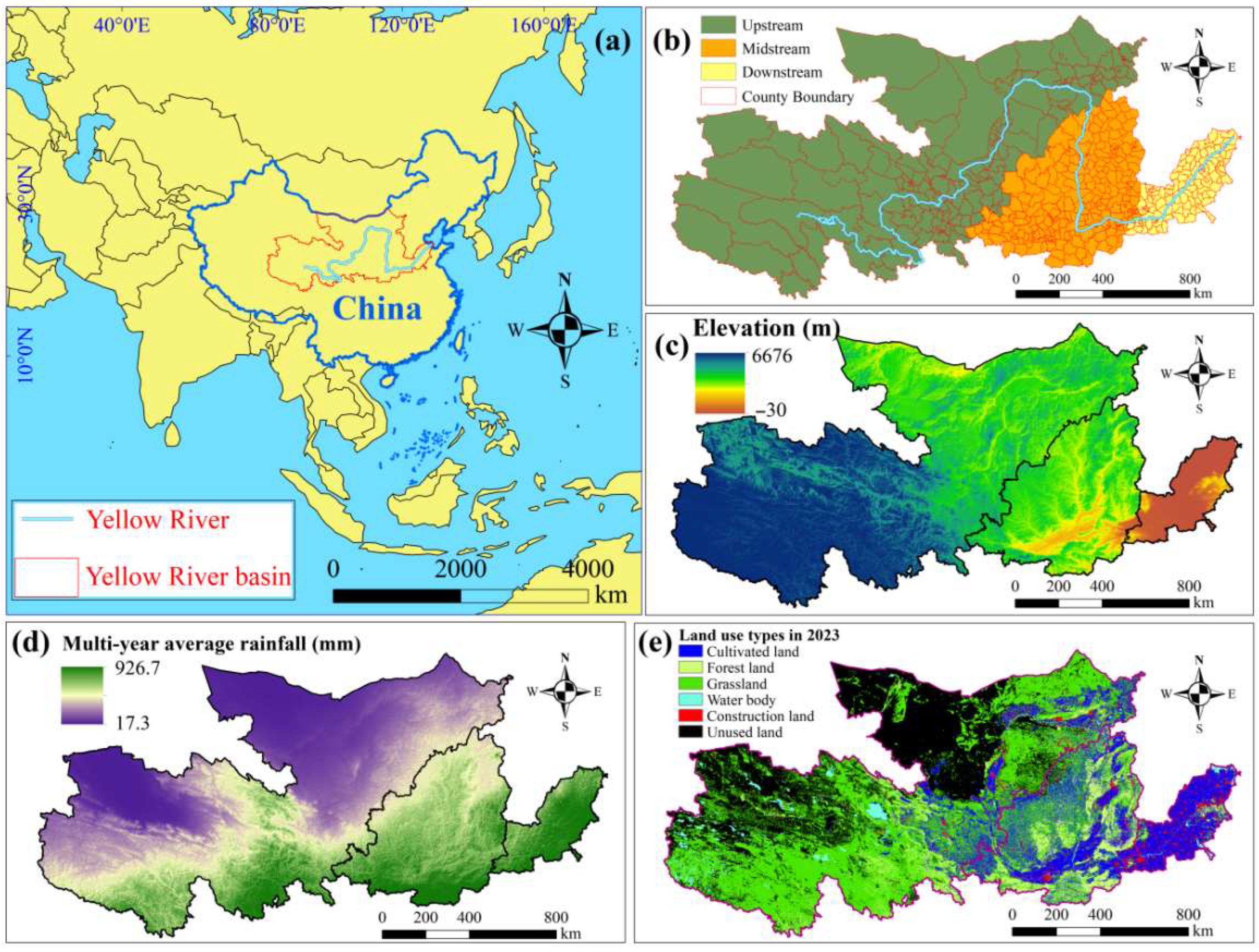
Figure 1. Study area location (a), administrative division (b), elevation (c), rainfall (d), and land use type (e) of the YRB.
Remotesensing 17 03028 g001
Figure 2. Flow chart of this study (NPP: net primary production; SE: soil erosion negative service; CS: carbon sequestration; WY: water yield).
Remotesensing 17 03028 g002
Figure 3. Spatial variation in 2000 (a), 2010 (b), 2023 (c) and temporal variation (d) of soil erosion negative service (The dashed lines of different colors are respectively the trend lines of the corresponding regions).
Remotesensing 17 03028 g003
Figure 4. Spatial variation in 2000 (a), 2010 (b), and 2023 (c) and temporal variation (d) of carbon sequestration (The dashed lines of different colors are respectively the trend lines of the corresponding regions).
Remotesensing 17 03028 g004
Figure 5. Spatial variation in 2000 (a), 2010 (b), and 2023 (c) and temporal variation (d) of water yield (The dashed lines of different colors are respectively the trend lines of the corresponding regions).
Remotesensing 17 03028 g005
Figure 6. Pearson correlation coefficient among ES pairs (SE: soil erosion negative service; CS: carbon sequestration; WY: water yield; ** means p < 0.01; blue arrows indicate that relationships are development in a synergistic direction, while red arrows indicate that relationships are development in a tradeoff direction).
Remotesensing 17 03028 g006
Figure 7. Spatial distribution (a) and area ratio (b) of tradeoff/synergy among ES pairs (SE: soil erosion negative service; CS: carbon sequestration; WY: water yield).
Remotesensing 17 03028 g007
Figure 8. Discretization results for continuous variables (SOC: soil organic carbon content; CLAY: clay content; SAND: sand content; SILT: silt content; ELE: average elevation; SLO: average slope; TEM: annual average temperature; RAIN: annual average rainfall; EVA: annual average evapotranspiration; PFA: proportion of farmland; PFG: proportion of forestland and grassland; FVC: fractional vegetation cover; POP: population density; GDP: GDP density; HAI: human activity intensity).
Remotesensing 17 03028 g008
Figure 9. The driving force of tradeoff/synergy for SE-CS (a), SE-WY (b), CS-WY (c) and Legend (d) (SE: soil erosion negative service; CS: carbon sequestration; WY: water yield; SE-CS: the relationships between SE and CS; SE-WY: the relationships between SE and WY; CS-WY: the relationships between CS and WY).
Remotesensing 17 03028 g009
Table 1. Assignment table for cultivated land.
Slope (°)≤55~1010~1515~202~25≥25
p value0.1000.2210.3050.5750.7050.800
Table 2. Details of latent drivers for investigating influences on interaction of ESs.
VariableLatent DriverAbbreviationUnit
Soil propertiesSoil organic carbon contentSOC%
Clay contentCLAY%
Sand contentSAND%
Silt contentSILT%
Topographic conditionsAverage elevationELEm
Average slopeSLO°
Climatic conditionsAnnual average temperatureTEM
Annual average rainfallRAINmm
Annual average evapotranspirationEVAmm
GFGPProportion of farmlandPFA%
Proportion of forestland and grasslandPFG%
Fractional vegetation coverFVC%
Socioeconomic situationsPopulation densityPOPpeople/km2
GDP densityGDP104 CNY/km2
Human activity intensityHAI-
Table 3. Detailed description and application of the data.
Data TypeDatasetFormatSourceApplication
Spatial vector dataAdministrative boundaries dataVector, CountyResource and Environmental Science Data Center (RESDC, http://www.resdc.cn/)For all analyses
Remote sensing dataLand use dataRaster, 1000 mRESDC (http://www.resdc.cn/)Soil erosion negative service calculation; water yield calculation; driver analysis
FVC dataRaster, 250 mNational Tibetan Plateau Data Center (https://data.tpdc.ac.cn/)Soil erosion negative service calculation; driver analysis
Net primary production dataRaster, 1000 mRESDC (http://www.resdc.cn/)Carbon sequestration calculation
Physical geographical dataClimate-related dataRaster, 1000 mNational Earth System Science Data Center (http://www.geodata.cn/)Soil erosion negative service calculation; water yield calculation; driver analysis
Digital Elevation Model (DEM) dataRaster, 30 mGeospatial Data Cloud (http://www.gscloud.cn/)Soil erosion negative service calculation; driver analysis
Soil dataRaster, 1000 mNational Cryosphere Desert Data Center (http://www.ncdc.ac.cn/portal/)Soil erosion negative service calculation; water yield calculation; driver analysis
Socioeconomic dataPopulationSpreadsheet, countyChina Statistical Database (https://www.shujuku.org/, accessed on 12 March 2025)Driver analysis
GDPSpreadsheet, countyChina Statistical Database (https://www.shujuku.org/, accessed on 12 March 2025)Driver analysis
Disclaimer/Publisher’s Note: The statements, opinions and data contained in all publications are solely those of the individual author(s) and contributor(s) and not of MDPI and/or the editor(s). MDPI and/or the editor(s) disclaim responsibility for any injury to people or property resulting from any ideas, methods, instructions or products referred to in the content.