Article

HTMNet: Hybrid Transformer–Mamba Network for Hyperspectral Target Detection

1
School of Aerospace Science and Technology, Xidian University, Xi’an 710126, China
2
Xi’an Institute of Space Radio Technology, Xi’an 710100, China
*
Author to whom correspondence should be addressed.
Remote Sens. 2025, 17(17), 3015; https://doi.org/10.3390/rs17173015
Submission received: 7 July 2025 / Revised: 16 August 2025 / Accepted: 26 August 2025 / Published: 30 August 2025
(This article belongs to the Special Issue Advances in Remote Sensing Image Target Detection and Recognition)

Abstract

Hyperspectral target detection (HTD) aims to identify pixel-level targets within complex backgrounds, but existing HTD methods often fail to fully exploit multi-scale features and integrate global–local information, leading to suboptimal detection performance. To address these challenges, a novel hybrid Transformer–Mamba network (HTMNet) is proposed to reconstruct the high-fidelity background samples for HTD. HTMNet consists of the following two parallel modules: the multi-scale feature extraction (MSFE) module and the global–local feature extraction (GLFE) module. Specifically, in the MSFE module, we designed a multi-scale Transformer to extract and fuse multi-scale background features. In the GLFE module, a global feature extraction (GFE) module is devised to extract global background features by introducing a spectral–spatial attention module in the Transformer. Meanwhile, a local feature extraction (LFE) module is developed to capture local background features by incorporating the designed circular scanning strategy into the LocalMamba. Additionally, a feature interaction fusion (FIF) module is devised to integrate features from multiple perspectives, enhancing the model’s overall representation capability. Experiments show that our method achieves AUC(PF, PD) scores of 99.97%, 99.91%, 99.82%, and 99.64% on four public hyperspectral datasets. These results demonstrate that HTMNet consistently surpasses state-of-the-art HTD methods, delivering superior detection performance in terms of AUC(PF, PD).

1. Introduction

Hyperspectral remote sensing employs a combination of imaging and spectral techniques, enabling the acquisition of detailed spectral information for every pixel over a wide wavelength spectrum, producing hyperspectral images (HSIs) with numerous contiguous bands [1]. Due to their high spectral resolution, HSIs possess strong material discrimination capabilities, making them valuable for applications such as target detection [2,3], classification [4,5], super resolution [6,7], anomaly detection [8,9], and unmixing [10,11], etc. Among these tasks, hyperspectral target detection (HTD) leverages spectral signatures to identify specific targets, and it has emerged as a research hotspot. Its capability for fine-grained spectral analysis enables accurate detection, even in complex background environments. As a result, HTD has found broad applications in areas such as military security [12,13], resource exploration [14,15], and environmental monitoring [16,17], etc. The core of HTD is to design effective detectors that exploit spectral discrepancies between different materials to enhance target visibility while minimizing background interference. Existing HTD approaches can be broadly categorized into the following two groups: traditional methods and deep learning (DL)-based methods.
Traditional HTD techniques primarily rely on matching-based approaches [18], such as spectral angular mapper (SAM) [19] and spectral information divergence (SID) [20], which use handcrafted decision functions to differentiate targets from backgrounds. SAM measures the angle between a test pixel and target spectra, while SID calculates the probability differences between spectra. However, these methods are prone to noise interference, which can degrade detection accuracy. In response, statistical distribution-based detection methods were introduced. The generalized likelihood ratio test (GLRT) [21] and related methods, such as the adaptive coherence estimator (ACE) [22], represent widely utilized approaches developed over the past few decades. In addition, methods like constrained energy minimization (CEM) [23] and related filters, like the target-constrained interference minimization filter (TCIMF) [24], function by optimizing energy equations based on energy minimization principles for target discrimination. Although these methods exhibit straightforward implementation procedures, real-world complexities often violate their underlying assumptions, limiting their effectiveness in practical applications.
To achieve greater performance in HTD, representation learning-based HTD methods are proposed. For example, Chen et al. [25] developed a sparsity-based algorithm for automatic HTD, leveraging the property that HSI pixels, lying in a low-dimensional subspace, can be expressed as sparse linear combinations of training pixels. Zhang et al. [26] introduced a novel sparse representation-based binary hypothesis network for HTD, which formulates the detection problem through a binary hypothesis framework grounded in the sparse representation characteristics. Li et al. [27] integrated sparse representation with collaborative representation to attain a more accurate background characterization. Zhang et al. [28] introduced a spatially adaptive sparse representation method for HTD, which incorporates neighboring spatial information by dynamically weighting the distinct contributions of surrounding pixels to enhance representation specificity. Zhao et al. [29] introduced a novel weighted Cauchy distance graph in conjunction with local adaptive collaborative representation, aiming to fully exploit spatial and spectral features. In addition, some other methods, including multiple instance learning [30], metric learning [31], and tensor decomposition [32,33], are proposed.
In recent years, DL-based approaches, especially those employing background reconstruction, have demonstrated satisfactory performance on HTD benchmark datasets [34]. For example, Tian et al. [35] devised a novel background reconstruction model by introducing the orthogonal subspace into a variational autoencoder (AE) to discern the background distribution. Sun et al. [36] introduced an adaptive background adversarial learning strategy aimed at enhancing the accuracy of background modeling. Leveraging adversarial learning, Qin et al. [37] proposed a novel two-stage detection framework that utilizes weakly supervised background reconstruction to extract spectral features from the latent space.
For discriminative feature extraction, some deep learning-based HTDs mainly employed convolutional neural network (CNN) to capture spatial and local features. For example, Gao et al. [38] developed a dual-branches network by introducing generative adversarial network (GAN) and CNN to focus on spectral and spatial features. In addition, Xu et al. [39] combined graph neural network (GNN) and CNN to improve the performance of HTD. However, CNN-based methods may exhibit limitations in capturing global contextual information, potentially constraining overall model performance. Therefore, some researchers have attempted to model global features by introducing Transformer. For example, Qin et al. [40] developed an integrated spectral–spatial framework, leveraging the Transformer architecture for the purpose of learning spectral–spatial features. Rao et al. [41] developed a Siamese Transformer network to suppress the background and highlight the targets. Jiao et al. [42] proposed a triplet spectral-wise Transformer-based model to learn local features and global features. Recently, Mamba [43] has obtained attention for modeling long sequences with linear complexity. Based on this, Shen et al. [44] introduced a pyramid state space model (SSM) which served as the backbone network, enabling the capture and fusion of multi-resolution spectral features, thereby alleviating spectral variation and enhancing robust representation.
Although recent Transformer- and Mamba-based methods have achieved promising results in HTD, some critical challenges remain. First, many existing methods do not adequately exploit multi-scale features, which limits cross-scale feature interaction and reduces the ability to capture diverse spatial patterns. Second, current approaches often fail to effectively integrate global and local contextual information, leading to incomplete background representations and reduced discrimination between targets and complex backgrounds. Third, some methods are unable to fully fuse the extracted multi-perspective features, which may cause semantic gaps between different feature sources and weaken the overall representation capability. Addressing these challenges is essential for improving background modeling accuracy, enhancing target discrimination, and achieving robust detection performance in real-world scenarios. In response to these difficulties, we propose a novel hybrid Transformer–Mamba network (HTMNet) for modeling high-fidelity background samples in HTD. HTMNet comprises the following two parallel modules: a multi-scale feature extraction (MSFE) module and a global–local feature extraction (GLFE) module, aimed at capturing background features from multiple perspectives. Specifically, the MSFE module utilizes Transformer-based architecture for the extraction and integration of multi-scale background features. In the GLFE module, a global feature extraction (GFE) module integrates a spectral–spatial attention mechanism into the Transformer to capture global background features, while a local feature extraction (LFE) module is developed to capture local background features by incorporating the designed circular scanning strategy into the LocalMamba [45]. Our circular scanning strategy aggregates features from four corner-to-center circular trajectories, allowing for a more balanced coverage of surrounding spatial dependencies. This approach preserves locality while maintaining continuity across directions, thus alleviating the boundary discontinuity issue inherent in standard window partitions. Additionally, a feature interaction fusion (FIF) module is designed to achieve the interaction of multiple perspective features, further improving the fidelity of background modeling.
Apart from integrating Mamba and Transformer modules, the main innovation of HTMNet lies in its dual-branch architecture (MSFE + GLFE) and the FIF mechanism, which jointly address the limitations of existing HTD methods in both multi-scale representation and global–local feature modeling. This design enables HTMNet to capture complementary background features from multiple perspectives and to effectively fuse them for high-fidelity background modeling.
The key contributions of this paper are outlined below:
  • A novel HTMNet is designed for HTD, which effectively models high-fidelity background samples by jointly leveraging Transformer and Mamba architectures. This hybrid design significantly improves the network’s capability to distinguish target information from complex background by capturing both multi-scale and global–local features.
  • A dual-branch architecture is designed, consisting of an MSFE module and a GLFE module. The MSFE module employs a Transformer-based strategy to capture and fuse features at multiple spatial scales. The GLFE module further complements this by capturing global background features through incorporating a spectral–spatial attention module into the Transformer and extracting local background features via a novel circular scanning strategy embedded within the LocalMamba. This dual-perspective design can capture background features from multiple perspectives, enhancing both multi-scale and global–local representation capabilities.
  • A FIF module is further devised to facilitate the integration and interaction of features extracted from the two branches. By promoting multi-scale and global–local feature fusion, the FIF module enhances contextual consistency and semantic complementarity among features, enhancing background modeling accuracy and robustness.
The remainder of this paper is structured as follows. Section 2 covers the foundational concepts of Mamba and details the proposed HTMNet. Section 3 details the experimental setup, presents the results, and provides the corresponding analysis. Section 4 and Section 5 describe the discussion and conclusion of this paper, respectively.

2. Methods

We propose a novel HTMNet to overcome the limitations of existing HTD methods in capturing multi-scale and global–local features. The HTMNet is designed to model high-fidelity background representations by utilizing the complementary advantages of Transformer and Mamba architectures. As shown in Figure 1, the overall framework consists of the following three main components: MSFE, GLFE, and FIF modules. Specifically, the MSFE module that leverages Transformer-based mechanisms to capture and fuse features across different spatial scales. The GLFE module further complements this by capturing global background features through incorporating a spectral–spatial attention module into Transformer and extracting local background features via a novel circular scanning strategy embedded within the LocalMamba. To integrate these complementary features, a FIF module is introduced, enabling effective multi-scale and global–local information interaction. This architecture allows HTMNet to model high-fidelity background representations, thereby improving detection performance in complex scenes.

2.1. Preliminary

In recent times, the state space model (SSM) has drawn considerable interest within the domain of sequential data modeling [43]. These models are typically derived from continuous-time dynamical systems; here, the system transforms input sequence x ( t ) R L into output sequence y ( t ) R L through a latent state h ( t ) R N . Here, N and L represent separately the dimensions of the latent space and input sequence. The underlying process can be characterized by the following linear ordinary differential equations (ODEs):
h ( t ) = A h ( t ) + B x ( t ) y ( t ) = C h ( t )
where h ( t ) denotes the time derivative of h ( t ) ; A R N × N , B R N × L , and C R L × N denote the system parameters. To integrate the continuous SSM into deep learning algorithms, it is crucial to carry out the discretization process. In particular, the ODEs given in Equation (1) are discretized through the application of the zero-order hold rule, as demonstrated below:
h t = A ¯ h t 1 + B ¯ x t y t = C h t
The computation of matrices A ¯ R N × N and B ¯ R N × L is calculated as follows:
A ¯ = exp ( Δ A ) B ¯ = ( Δ A ) 1 ( exp ( Δ A I ) ) Δ B
where Δ represents a timescale factor, striking a balance between the impact of the present input and the previous state. In actual implementation, B ¯ is approximated as Δ B according to the first-order Taylor series expansion.
However, the capacity of SSMs to capture sequence context is inherently limited due to their static parameterization. To overcome this limitation, Mamba [43] takes a step further by improving state interaction through the introduction of a selective mechanism (S6). This mechanism can more effectively identify key dependencies within sequences. The success of such advancements has opened doors for their application in vision-related fields. For example, VMamba [46] introduced an innovative 2D selective scanning approach (SS2D). This approach scans images in both horizontal and vertical directions, ultimately enhancing the model’s performance.

2.2. Preprocessing Module

To obtain more robust input, we first perform preprocessing on the input HSI. Specifically, given an original HSI X o H × W × B , where H and W signify, separately, the height and width of HSI, and B signifies the number of spectral bands. Each pixel x i , j o B denotes the spectral vector situated at coordinate ( i , j ) . For a certain pixel x i , j o in HSI, we extract its surrounding spatial patch. Assuming the patch size is K × K , the patch can be formulated as follows:
P i , j = { x i + m , j + n o | m , n { K 1 2 , , K 1 2 } }
where P i , j K × K × B is the patch centered at ( i , j ) and x i + m , j + n o is the spectral vector within the patch. By encoding all pixels using spectral similarity, we obtain the enhanced spectral vector x , as follows:
x = P T W
where W K × K signifies the similarity weight matrix between the central pixel and surrounding pixels. The similarity weight w i W for the i-th pixel is defined below:
w i = exp ( s ( x c o , P i ) ) j = 1 K 2 exp ( s ( x c o , P j ) )
where x c o represents the central pixel in patch P and s ( ) denotes the cosine similarity function. Similarly, according to Equation (5), we calculate all pixels in the original HSI to derive the enhanced HSI X H × W × B .

2.3. Multi-Scale Feature Extraction Module

To extract and fuse multi-scale spatial features, the MSFE module is designed, as illustrated in Figure 1b. Specifically, in the bottom-up downsampling process, the spatial size is gradually reduced (downsampled by a factor of 2) to obtain multi-scale representations by using the convolution and average pooling operation, as follows:
X k = Avgpool ( Conv 3 × 3 ( X k 1 ) )
where k { 1 , 2 , 3 } , X 0 = X , Conv 3 × 3 ( ) denotes the convolution with kernel 3 and Avgpool ( ) denotes the average pooling operation.
After each downsampling, the multi-head self-attention module is applied to the corresponding feature maps, as detailed in Figure 2, which corresponds to the module illustrated in Figure 1b. Specifically, taking X H × W × B as an example, first, linear projections are used to project X into query Q H × W × B , key K H × W × B , and value V H × W × B . The above calculation can be defined below, as follows:
Q = X W Q , K = X W K , V = X W V
where W Q , W K , W V B × B denote the learnable weights. Second, Q , K , and V are reshaped into two-dimensional forms through the Reshape operation Q , K , V B × H W , and they are partitioned into h self-attention heads along the channel direction, resulting in Q = [ Q 1 , Q 2 , , Q i , , Q h ] , K = [ K 1 , K 2 , , K i , , K h ] , and V = [ V 1 , V 2 , , V i , , V h ] . Here, the dimension of each attention head is C/h. For each group of Q i , K i , V i , the Softmax function is employed to calculate the multi-head self-attention score, as follows:
Y i = Softmax ( Q i ( K i ) T α ) V i
where Y i signifies the output of the i-th head in the self-attention mechanism and α denotes the learnable scalar. Finally, use Concatenation and Reshape operations to merge the outputs of all heads and restore their shapes to obtain Y k H × W × B , k { 0 , 1 , 2 , 3 } .
In the top-down upsampling process, the spatial size is increased by a factor of 2, gradually restoring the original size. Each upsampling step is followed by combining the upsampled feature maps with the corresponding feature maps from the multi-head self-attention block. The formulation of the process is presented below.
F M S = Y 0 + TConv 3 × 3 ( Y 1 + TConv 3 × 3 ( Y 2 + TConv 3 × 3 ( Y 3 ) ) )
where TConv 3 × 3 ( ) denotes the transposed convolution with kernel 3.
In summary, the MSFE module processes the input through a series of downsampling and upsampling stages, integrating multi-head self-attention at each stage to enhance feature representation and capture multi-scale features.

2.4. Global–Local Feature Extraction Module

To extract global–local features, a novel GLFE module is devised, as illustrated in Figure 1c. In the GLFE module, a GFE module integrates a spectral–spatial attention mechanism into the Transformer to capture global background features, while an LFE module utilizes a novel circular scanning strategy within the LocalMamba [45] to extract fine-grained features. The details of the GFE and LFE modules are as follows.

2.4.1. Global Feature Extraction Module

The GFE module is designed to capture global background features, as shown in Figure 1c. Specifically, the GFE module consists of a self-attention module and a spectral–spatial attention module. To be specific, given input X H × W × B , the GFE module firstly obtains its embedding features Q , K , V H × W × B and A H × W × B through convolution projection, as follows:
Q , K , V , A = Split ( DConv 3 × 3 ( Conv 1 × 1 ( LN ( X ) ) ) )
where LN ( ) represents the layer normalization, Conv 1 × 1 ( ) signifies the convolution layer with kernel 1, DConv 3 × 3 ( ) signifies the depth-wise convolution with kernel 3, and Split ( ) denotes the split operation. Then, the global background features F G H × W × B are obtained as follows:
F G = F S A + F S S + X
where F S A = Softmax ( Q K T α ) V denotes the output of the self-attention module. F S S H × W × B denotes the output of the spectral–spatial attention module. The details of the spectral–spatial attention module are as follows:
(1)
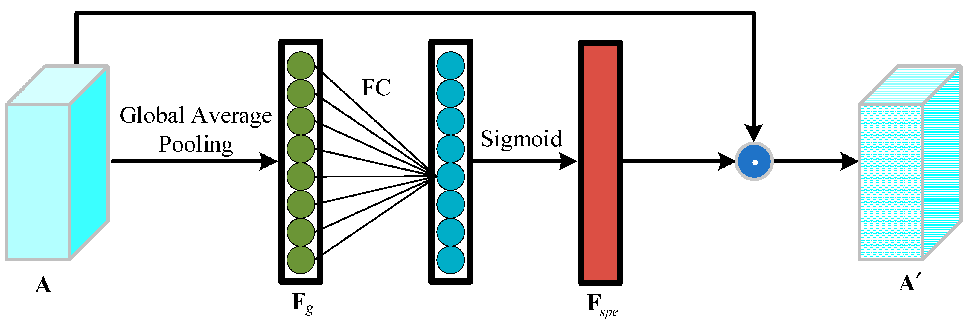
Spectral attention module: Figure 3 corresponds to the spectral attention module in Figure 1c, specifically, first, a global average pooling operation is performed on the features A to obtain the global feature representation F g 1 × 1 × B of each channel. Then, the F g is imported into the fully connected (FC) layer and Sigmoid function to obtain spectral attention weights F s p e 1 × 1 × B . Finally, we obtain the enhanced spectral features A H × W × B by element-wise multiplication of F s p e and A . The processes are formulated as follows.
F g = GAP ( A ) F s p e = Sigmoid ( FC ( F g ) ) A = A F s p e
where GAP ( ) signifies the global average pooling layer, FC ( ) signifies the FC layer, Sigmoid ( ) represents the Sigmoid activation function, and denotes the element-wise multiplication.
(2)
Spatial attention module: Figure 4 corresponds to the spatial attention module in Figure 1c, specifically, first, a max and average of the pooling layers are performed on the features A to obtain pooled features F m H × W × 1 and F a H × W × 1 . Then, after concatenating F m and F a , a convolution followed by a Sigmoid function is performed to attain the spatial attention features F s p a H × W × 1 . Finally, we obtain the output F S S H × W × B of the spectral–spatial attention module by element-wise multiplication of F s p a and A . The processes are formulated as follows.
F m = MP ( A ) , F a = AP ( A ) F s p a = Sigmoid ( Conv 3 × 3 ( Concat ( F m , F a ) ) ) F S S = A F s p a
where MP ( ) signifies the max pooling layer, AP ( ) signifies the average pooling layer, Concat ( ) denotes the concatenate operation along the channel dimension, and Conv 3 × 3 ( ) denotes the convolution with kernel 3.

2.4.2. Local Feature Extraction Module

The inherent non-causality of 2D spatial data in images poses a fundamental challenge to methods designed for causal processing. Conventional techniques that flatten spatial tokens often disrupt local 2D structural relationships, thereby weakening the model’s capacity to effectively capture spatial dependencies. For example, the flattening strategy used in Vim [47] increases the separation between vertically adjacent tokens, undermining local coherence and impairing the model’s sensitivity to spatial details. Although VMamba [46] mitigates this issue by applying bidirectional scans (both horizontally and vertically), it still struggles to capture complete spatial contexts in a single pass. To handle the limitation, LocalMamba [45] presents an innovative method for local image scanning that partitions images into multiple local windows, facilitating the closer arrangement of pertinent local tokens, and thereby improving the modeling of local dependencies. However, the existing scanning strategy disrupts local spatial continuity, making it less effective for modeling local information. To tackle this challenge, we propose a circular scanning strategy to flatten the local image into a 1D sequence, as illustrated in Figure 5.
Based on the above analysis, an LFE module based on LocalMamba is devised to capture local background features, as illustrated in Figure 1c. Specifically, circular scanning along four distinct directions is first applied to flatten the local image into a 1D sequence. Subsequently, four distinct S6 blocks are employed to learn rich feature representations from each direction. To enhance feature integration and filter out irrelevant information, we adopt the spatial-channel attention (SCA) module, following the design in LocalMamba [45]. This module utilizes two components, channel attention and spatial attention, to dynamically assign weights to feature channels and spatial locations. Finally, the outputs of the four SCA modules are merged to obtain the local background feature F L .
Finally, the global–local background features are attained using the dynamic weight fusion mechanism, as follows:
F G L = w 1 F G + w 2 F L
where w 1 and w 2 denote the learnable parameters.

2.5. Feature Interaction Fusion Module

To model more robust background samples, a FIF module is designed to enhance and integrate two input features, F M S and F G L , through cross-branch interaction, as illustrated in Figure 1d. Specifically, each input is first processed by both max and average pooling operations to extract complementary statistical features. The pooled outputs are then concatenated and passed through a convolutional layer to acquire compact representations F 1 and F 2 . These representations are used to modulate the original features via cross-wise multiplication (i.e., the F 1 is multiplied with F M S , and vice versa), enabling mutual enhancement between the two branches. The resulting features are then added back to their respective original inputs, and finally, the two updated features F ^ M S and F ^ G L are fused through the element-wise addition to produce the output feature X ^ .
F 1 = Conv 3 × 3 ( Concat ( MP ( F G L ) , AP ( F G L ) ) ) F 2 = Conv 3 × 3 ( Concat ( MP ( F M S ) , AP ( F M S ) ) ) F ^ M S = ( F 1 F M S ) + F M S F ^ G L = ( F 2 F G L ) + F G L X ^ = F ^ M S + F ^ G L
where MP ( ) signifies the max pooling layer, AP ( ) signifies the average pooling layer, Concat ( ) signifies the concatenate operation along channel dimension, and Conv 3 × 3 ( ) denotes the convolution with kernel 3.

2.6. Model Training and Inference

In the training stage, the L2 norm is utilized as the loss function L to train the HTMNet, which is shown below:
L = 1 H W w i j i = 1 H j = 1 W x i j x ^ i j 2
where 2 represents the L2 norm, x i j denotes the enhanced spectral vector at coordinates (i, j), and x ^ i j denotes the reconstructed spectral vector at coordinates (i, j). w i j denotes the similarity weight, which is introduced to suppress the reconstruction of targets. Specifically, the w i j is obtained by calculating the cosine similarity between target spectrum y and enhanced spectral vector x i j .
w i j = exp x i j y T x i j 2 y 2
In the inference stage, the enhanced HSI X is imported into the trained HTMNet to acquire the reconstructed HSI X ^ ; the detection result can be obtained as follows:
R = N max min X X ^ 2
where N max min denotes the max–min normalization. Finally, nonlinear background suppression is employed to suppress the background, as follows:
R = exp ( R 1 ) 2 α
where α is a hyperparameter that controls the degree of background suppression.

3. Results

3.1. Experimental Setup

3.1.1. Dataset Setup

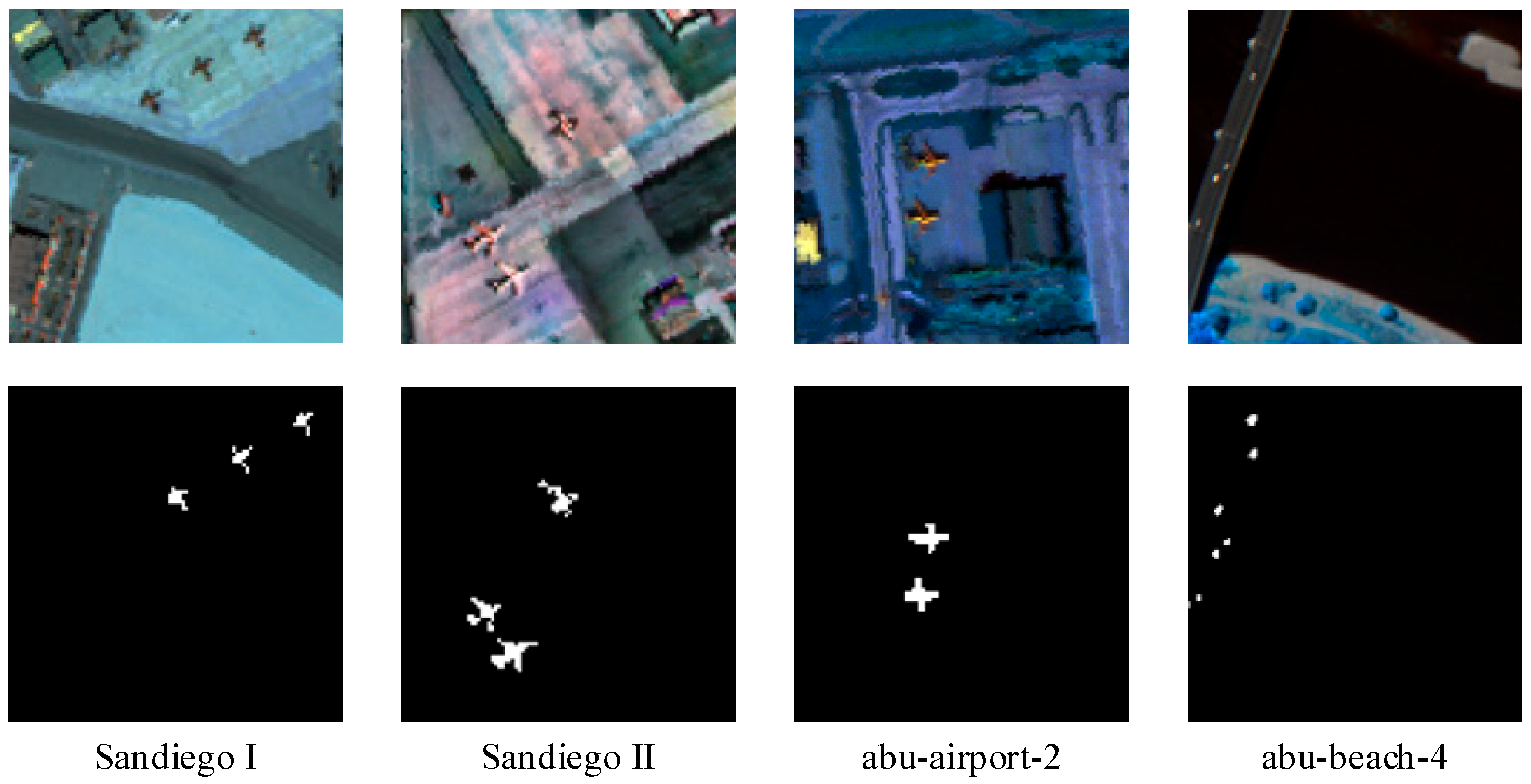
We evaluated the proposed HTMNet on four publicly available HSIs. Details regarding these datasets are presented below, while Figure 6 shows false-color images alongside their corresponding ground truth (GT) maps.
(1)
San Diego I and San Diego II [48]: The first two datasets, San Diego I and San Diego II, were acquired using the Airborne Visible Infrared Imaging Spectrometer (AVIRIS) at San Diego Airport, California, USA. Both HSIs have dimensions of 100 × 100 × 224, featuring a spatial resolution of 3.5 m and covering the wavelength range from 400 to 2500 nm. Following the removal of low-quality bands, 189 spectral bands were retained for the experimental analysis. The targets to be inspected are three aircraft.
(2)
Abu-airport-2 [49]: The third dataset, Abu-airport-2, was collected by AVIRIS on the Los Angeles Airport scene in California. The size of HSI is 100 × 100 × 205, featuring 100 × 100 pixels and 205 spectral bands, with a wavelength range of 400 to 2500 nm. Spatial resolution of this dataset is 7.1 m. The targets to be detected are two aircraft, consisting of 87 pixels.
(3)
Abu-beach-4 [49]: The fourth dataset, Abu-beach-4, was collected by the Reflectometry Imaging Spectrometer (ROSIS-03) sensor in the Pavia Beach area of Italy. The spatial size of HSI is 150 × 150 and the spatial resolution is 1.3 m. It consists of 115 spectral bands, ranging from 430 nm to 860 nm. After removing the low-quality bands, there were still 102 bands in the experiment. Some Vehicles on the bridge are marked as targets.
In the experiment, the pixel that is closest to the average spectrum of all the target pixels is selected as the target spectrum.

3.1.2. Evaluation Metric

The performance of HTD models is assessed in this article through comprehensive qualitative and quantitative evaluation measures. For qualitative measure, this paper adopts the 3D receiver operating characteristic (ROC) curve [50,51], background-target separation map, and visual detection map to intuitively compare the detection performance. For quantitative evaluation, three AUC values, AUC(PF, PD), AUC(τ, PD), and AUC(τ, PF), are defined as the integrations of their corresponding ROC curves, which are as follows: ROC(PF, PD), ROC(τ, PD), and ROC(τ, PF), where PF, PD, and τ denote, separately, false-alarm probability, detection probability, and threshold. Based on these, two additional AUC metrics are further derived through the following formulations:
AUC SNPR = AUC ( τ , P D ) AUC ( τ , P F ) AUC ODP = AUC ( P F , P D ) + AUC ( τ , P D ) AUC ( τ , P F )
where AUC ODP and AUC SNPR denote the overall detection probability and signal-to-noise probability ratio, respectively.

3.1.3. Implementation Details

In this article, we construct the single-scale feature extraction (SSFE) network as the baseline by removing the GLFE module, FIF module, and multi-scale module in MSFE. The input HSI data are normalized to the range [0, 1] using min–max normalization before training, and no data augmentation is applied. The batch size is set to the total number of pixels in the corresponding dataset, allowing all pixels to be processed in a single optimization step. The L2 norm is used as the training objective. The AdamW optimizer is adopted for training, with a weight decay of 10−4. Learning rate is set to 1 × 10⁻⁴, gradually increasing during the first 10% of epochs using a linear warm-up scheduler, and subsequently decreasing following a cosine schedule. The training epochs are set to 200. In the background suppression procedure, the parameter α is set to 0.1 on four HSI datasets. The head H in MSFE is set to 2. The patch sizes P of the center pixel are set to 11 × 11, 13 × 13, 11 × 11, and 5 × 5 for San Diego I, San Diego II, Abu-airport-2, and Abu-beach-4. The parameters H and patch size P are quantitatively analyzed in Section 4.5.
The experiments were performed using Python 3.10 and PyTorch 2.0, running on a system featuring an Intel® Core™ i7-6700 CPU, 32 GB of RAM, and an NVIDIA RTX 5880 Ada Generation GPU with 48 GB of memory.

3.2. Ablation Study

An ablation study with different configurations is conducted to evaluate the influence of the proposed MSFE, GLFE, and FIF modules. Specifically, as shown in Table 1, the first row signifies the baseline model. The second row denotes baseline with the multi-scale module (i.e., MSFE). The third row combines the MSFE and GLFE modules. The final row demonstrates the proposed method, which incorporates the MSFE, GLFE, and FIF modules.
(1)
Effectiveness of MSFE: To assess the effectiveness of MSFE, we conducted an experiment by integrating the multi-scale module into the baseline. As shown in Table 1, MSFE outperforms the baseline by 0.74%, 0.58%, 0.35%, and 0.26% on the four datasets, respectively, demonstrating its effectiveness. These improvements indicate that MSFE is capable of effectively extracting multi-scale features for better background modeling.
(2)
Effectiveness of GLFE: To assess the effectiveness of GLFE, we conducted an experiment by combining MSFE and GLFE, where their outputs were added directly to obtain the final result. As shown in Table 1, MSFE + GLFE outperforms MSFE alone by 0.08%, 0.09%, 0.21%, and 0.65% on the four datasets, respectively. These results show that GLFE is effective in capturing complementary global and local contextual information, which further enhances the representational capability of the model.
(3)
Effectiveness of FIF: By incorporating the FIF module to fuse the outputs of MSFE and GLFE, we conducted an experiment aimed at assessing the effectiveness of FIF. As shown in Table 1, the configuration MSFE + GLFE + FIF outperforms MSFE + GLFE by 0.03%, 0.02%, 0.10%, and 0.32% on the four datasets, respectively. These results demonstrate that FIF effectively enhances feature interaction and fusion, contributing to improved detection performance.
The main performance gains of HTMNet come from the MSFE and GLFE modules, which directly enhance the network’s capacity to capture discriminative background features at multiple scales and perspectives. In contrast, the FIF module plays a complementary role, its primary function is to facilitate effective integration between the multi-scale features from MSFE and the global–local features from GLFE, ensuring contextual consistency and semantic complementarity.
Since FIF focuses on feature refinement and interaction rather than primary feature extraction, its impact appears as a consistent but moderate improvement in quantitative results. However, our ablation studies confirm that removing FIF leads to a decline in performance stability across datasets, especially in challenging scenes where background complexity and target similarity are high. Therefore, even though its numerical gain is smaller, FIF remains crucial for enhancing background modeling accuracy and robustness in the final model.

3.3. Comparison with Other Advanced HTD Methods

To prove the superiority of the proposed HTMNet, we conduct qualitative and quantitative comparisons with several advanced HTD methods, including CEM [23], CTTD [52], TD_TSE [53], TSTTD [42], HTD-IRN [54], and HTD-Mamba [44].

3.3.1. Qualitative Comparison

(1)
ROC curve comparisons
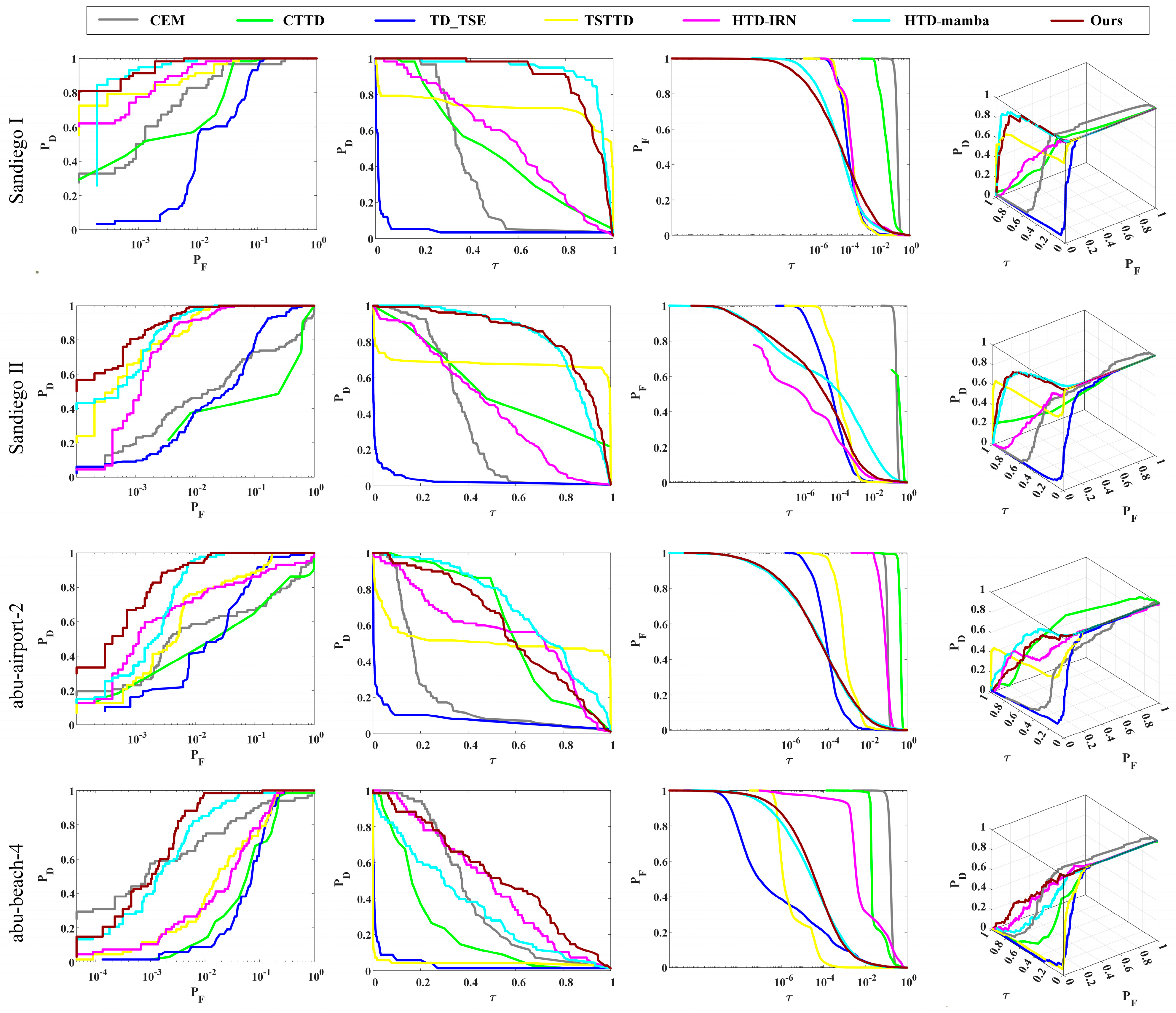
Figure 7 illustrates the ROC curves corresponding to different HTD methods, as evaluated across four HSI datasets. In the first column, the ROC(PF, PD) curve of HTMNet is closer to the upper-left corner, demonstrating its superior overall performance compared to other HTD methods. In the second column, the ROC(τ, PD) curve of HTMNet is closer to the upper-right corner on the San Diego II and Abu-beach-4 datasets, indicating its superior detection probability compared to other HTD methods. Moreover, it also achieves competitive results on the remaining datasets. In the third column, compared to other HTD methods, HTMNet achieves a more leftward ROC(τ, PF) curve, demonstrating its effectiveness in reducing false-alarm rates. Additionally, the fourth column shows the 3D ROC curves (τ, PF, PD), further validating the effectiveness of HTMNet.
(2)
Background-target separation map comparisons
To further evaluate the background-target separation performance of each method, Figure 8 presents the separation maps of seven methods across four HSI datasets. In the maps, red and blue boxes signify the distributions of targets and background, respectively. A larger gap between these boxes indicates better separability. As shown in Figure 8, HTMNet exhibits superior background-target separation on San Diego II and Abu-beach-4 datasets, and maintains competitive separation capability on San Diego I and Abu-airport-2 datasets. Moreover, HTMNet demonstrates a background distribution range close to zero across four datasets, reflecting its strong background suppression ability compared to other HTD methods.
For Figure 8b,d, it can be observed that the proposed method achieves the best background-target separability, which is further validated by the quantitative metric AUC(τ, PD). As shown in Table 2, our method also obtains the highest AUC(τ, PD) values for these datasets. For Figure 8a,c, our method achieves competitive separability, which is consistent with its competitive AUC(τ, PD) values reported in Table 2. In addition, as shown in Figure 8, the background distributions of our method and some other methods are both close to zero, indicating that our method has a competitive background suppression capability. This observation is consistent with the AUC(τ, PF) metric in the quantitative analysis, as shown in Table 2, where our method also achieves competitive results.
(3)
Detection map comparisons
For an intuitive comparison, Figure 9 displays the visualized result maps of seven HTD methods on four HSI datasets. The results indicate that our proposed method obtains an optimal balance between target highlighting and background suppression. Specifically, the traditional method CEM struggles to accurately detect targets while effectively suppressing the background. HTD-IRN and HTD-Mamba can detect most target pixels but suffer from weak background suppression. Conversely, TD_TSE and TSTTD suppress background noise well but fail to retain complete target information. CTTD exhibits unstable performance, often missing useful information or producing excessive false-positives. In contrast, the proposed HTMNet consistently achieves accurate target localization and effective background suppression. Its detection maps closely align with the GT, preserving the shape and contour of the targets, thereby demonstrating superior detection performance.

3.3.2. Quantitative Comparison

To quantitatively assess model performance, Table 2 reports the AUC scores of all methods on four HSI datasets. As shown in Table 2, the proposed HTMNet consistently obtains the highest AUC(PF, PD) scores across all four HSI datasets, demonstrating its superior overall performance. For AUC(τ, PD), HTMNet achieves the highest scores across the San Diego II and Abu-beach-4 datasets, and obtains competitive results across the San Diego I and Abu-airport-2 datasets, highlighting its strong target detection capability. Regarding AUC(τ, PF), although TD_TSE and TSTTD perform well across all datasets, they suffer from severe loss of target information. In contrast, HTMNet maintains a favorable balance between background suppression and target detection by achieving competitive AUC(τ, PD) and AUC(τ, PF) scores. Additionally, our method achieves competitive AUCODP and AUCSNPR results on all datasets, indicating its comprehensive detection effectiveness.
Table 2 also compares the inference time of all methods, where CEM, CTTD, and TD_TSE exhibit faster inference due to their simpler architectures. Despite this, HTMNet achieves a competitive inference time among DL-based methods.
For the San Diego I and II datasets, the relatively homogeneous backgrounds and well-separated target spectra allow many methods to achieve high scores. As a result, our proposed model exhibits only small performance variations on these datasets.
For the Abu-beach-4 and Abu-airport-2 datasets, the more complex backgrounds lead to relatively lower detection performances for most HTD methods. However, due to the dual-branch architecture and the FIF module, HTMNet can help mitigate these effects by effectively capturing multi-scale and global–local features. As a result, our method is able to maintain high performance even in complex scenarios, which leads to more noticeable performance differences compared to other HTD methods.
In addition, baseline models also show large differences across datasets, because each dataset has different scene characteristics; for example, simpler backgrounds favor higher baseline performance, while complex backgrounds often result in poorer performance.
In summary, our method demonstrates outstanding detection performance and maintains competitive inference efficiency, achieving a favorable trade-off between accuracy and computational complexity.

4. Discussion

4.1. Impact of Fusion Strategy

To verify the superiority of the FIF module, we conducted additional experiments by comparing it to the following two alternative fusion strategies: (1) early fusion via pointwise addition, and (2) cross-attention fusion [55]. The results in Table 3 show that, although pointwise addition is computationally efficient, it yields only limited performance gains. Cross-attention fusion achieves accuracy comparable to FIF but incurs a substantially higher computational cost. In contrast, FIF achieves higher accuracy than both pointwise addition and cross-attention fusion, while maintaining low computational complexity, thereby offering a better trade-off between performance and efficiency.

4.2. Impact of the Larger Dataset

To assess the generalizability of HTMNet, we additionally evaluated it on a larger, widely used hyperspectral dataset, as shown in Figure 10a. The details of the dataset are as follows.
The SpecTIR dataset (larger dataset) [56] was collected from the SpecTIR hyperspectral airborne Rochester experiment (SHARE), with a spatial size of 180 × 180 pixels, 120 spectral bands, and 1 m spatial resolution. This dataset features a large spatial coverage and various background textures.
As shown in Table 4, for the SpecTIR dataset, HTMNet achieves the highest AUC(PF, PD) score, demonstrating a superior overall performance. For AUC(τ, PD), it also attains the highest score, highlighting its strong target detection capability. Regarding AUC(τ, PF), HTMNet yields lower false-alarm rates than other HTD methods. For AUCODP, HTMNet attains the highest scores among all compared methods. For AUCSNPR, HTMNet delivers competitive results compared to other HTD methods.
For an intuitive comparison, the first row of Figure 11 displays the visualized result maps of seven HTD methods on the SpecTIR dataset. Specifically, both HTMNet and HTD-Mamba can detect most target pixels; however, HTD-Mamba suffers more from weak background suppression than our method.
These results demonstrate that HTMNet achieves accurate target localization while maintaining effective background suppression, validating its generalizable detection performance on larger HSI dataset.

4.3. Impact of the Low-Contrast Dataset

To assess the generalizability of HTMNet, we additionally evaluated it on a low contrast, widely used hyperspectral dataset, as shown in Figure 10b. The details of the dataset are as follows:
The Salinas dataset (low contrast) [57] is acquired by the AVIRIS sensor; it covers the Salinas Valley region in California, USA, with a spatial size of 120 × 120 pixels, 204 spectral bands, and a spatial resolution of 3.7 m. Some targets in this dataset exhibit low contrast with the background, making them challenging to detect.
As shown in Table 4, for the Salinas dataset, HTMNet achieves the highest AUC(PF, PD) score, demonstrating a superior overall performance. For AUC(τ, PD), it attains competitive results. Regarding AUC(τ, PF), HTMNet achieves the lowest false-alarm rate, indicating effective background suppression. For AUCODP, it maintains a more competitive performance than other HTD methods, and for AUCSNPR, it attains the highest score among all compared methods.
For an intuitive comparison, the second row of Figure 11 displays the visualized result maps of seven HTD methods on the Salinas dataset. Specifically, HTMNet, HTD-IRN, and HTD-Mamba can detect the most target pixels, but HTD-IRN and HTD-Mamba exhibit higher false-alarm rates compared to our method.
These results confirm that HTMNet possesses a strong target detection capability and effective background suppression, and is able to distinguish between the targets and background, even when they share similar spectral or spatial characteristics.

4.4. Analyses of Computational Efficiency

We conducted additional experiments to compare the computational efficiency of deep learning-based HTD methods on the San Diego I dataset. As shown in Table 5, HTMNet exhibits the highest number of parameters, memory usage, and FLOPs among the compared methods. This higher complexity arises from the integration of the MSFE and GLFE modules, together with the FIF module. Despite the increased computational cost, these components collectively enhance the model’s capability to capture rich spatial–spectral patterns, thereby directly contributing to its superior detection accuracy.
HTMNet is designed with a focus on improving target detection accuracy. Compared to other HTD methods, HTMNet requires higher memory and FLOPs due to the dual-branch architecture and the incorporation of both Transformer- and Mamba-based modules. As such, the current version is not specifically optimized for deployment on highly resource-constrained platforms, such as satellites or unmanned aerial vehicles.
In future work, we plan to explore lightweight architectural variants of HTMNet, for example, by pruning redundant channels, employing low-rank approximations, or distilling a compact student model, to make the approach more suitable for real-time, edge, or on-board processing in satellite and UAV applications.

4.5. Impact of Hyperparameters

(1)
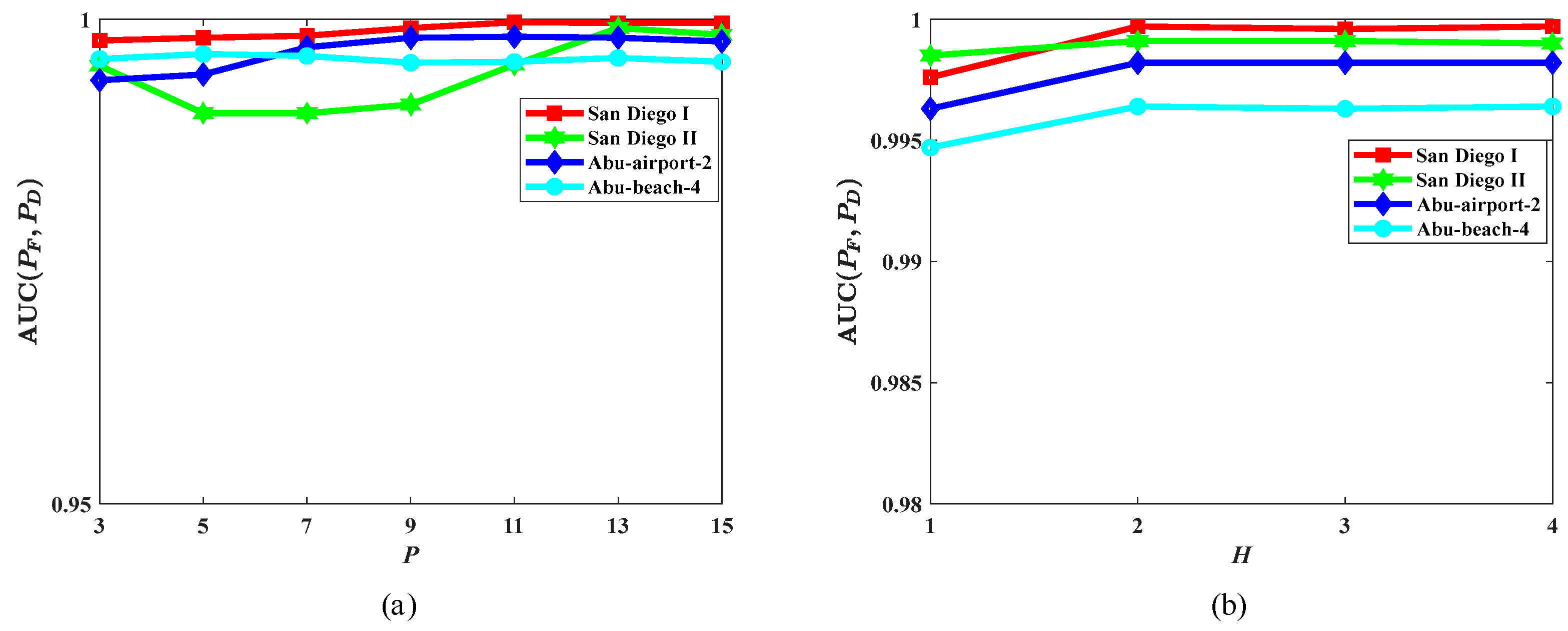
Patch size P: For the patch sizes, as shown in Figure 12a, the highest AUC(PF, PD) values were achieved when the patch sizes were set to 11 × 11, 13 × 13, 11 × 11, and 5 × 5 for the San Diego I, San Diego II, Abu-airport-2, and Abu-beach-4 datasets, respectively. Therefore, these sizes were adopted to ensure optimal detection performance for each dataset.
(2)
Number of attention heads H: For the number of attention heads, as shown in Figure 12b, when the number of attention heads exceeds 2, the AUC(PF, PD) value remains stable and reaches its maximum. Therefore, considering both detection accuracy and computational efficiency, the number of attention heads is set to 2.
(3)
For the scan orientations in the proposed circular scanning strategy, as illustrated in Figure 5, we designed four orientations starting from the four corner points and scanning towards the center in a circular manner. This configuration enables comprehensive local feature extraction from multiple perspectives.

4.6. Impact of Spectral–Spatial Attention (SSA) Block

To verify the effect of the spectral–spatial attention (SSA) block, we conducted the ablation experiments to verify its effect. Specifically, as shown in Table 6, removing the SSA block results in a decrease in detection accuracy, indicating its critical role in enhancing global feature extraction.

4.7. Impact of Similarity Strategy

To validate the impact of similarity, we conducted an additional experiment by replacing cosine similarity with Euclidean distance for spectral similarity computation. As shown in Table 7, using Euclidean distance led to lower detection accuracy compared to cosine similarity, confirming the superiority of cosine similarity for our task.

4.8. Differences with Existing Method

A method similar to our work is HTD-Mamba. HTD-Mamba primarily focuses on spectral sequence modeling using a pyramid state–space model and spectrally contrastive learning to enhance background-target discrimination. In contrast, HTMNet is a hybrid network combining Transformer and Mamba architectures, specifically designed to extract and integrate multi-scale and global–local features through its dual-branch structure, consisting of the MSFE and GLFE modules. Additionally, HTMNet designs a FIF module to promote contextual consistency and semantic complementarity between multi-perspective features, which is not present in HTD-Mamba.

5. Conclusions

In this article, we proposed a novel HTMNet for modeling high-fidelity background samples in HTD. HTMNet consists of two parallel modules—MSFE and GLFE—which is designed to capture background features from multiple perspectives. Specifically, the MSFE module employs a Transformer-based architecture to extract and fuse multi-scale background features. The GLFE module integrates a GFE submodule, which incorporates spectral–spatial attention into the Transformer, and an LFE submodule that utilizes a novel circular scanning strategy for LocalMamba to capture fine-grained local features. Furthermore, a FIF module is introduced to effectively integrate multi-perspective features, enabling accurate modeling of high-fidelity backgrounds. Ablation studies confirm the effectiveness of the MSFE, GLFE, and FIF modules. Extensive experimental results on four publicly available HSI datasets verify the effectiveness and superiority of the proposed HTMNet compared to advanced HTD approaches.

Author Contributions

X.Z., Y.K., Y.H. and W.Z. provided the methodology; X.Z. wrote the original draft; X.Z., Y.K., Y.H. and W.Z. performed experiments; and X.Z., Y.K., Y.H., W.Z., M.Z. and H.W. revised the manuscript. All authors have read and agreed to the published version of the manuscript.

Funding

This research received no external funding.

Data Availability Statement

The hyperspectral images used in this paper are available at http://xudongkang.weebly.com/ (accessed on 11 January 2013).

Conflicts of Interest

The authors declare no conflicts of interest.

References

  1. Tong, Q.; Xue, Y.; Zhang, L. Progress in hyperspectral remote sensing science and technology in China over the past three decades. IEEE J. Sel. Top. Appl. Earth Obs. Remote Sens. 2013, 7, 70–91. [Google Scholar] [CrossRef]
  2. Nasrabadi, N.M. Hyperspectral target detection: An overview of current and future challenges. IEEE Signal Process. Mag. 2013, 31, 34–44. [Google Scholar] [CrossRef]
  3. Chen, B.; Liu, L.; Zou, Z.; Shi, Z. Target detection in hyperspectral remote sensing image: Current status and challenges. Remote Sens. 2023, 15, 3223. [Google Scholar] [CrossRef]
  4. Audebert, N.; Le Saux, B.; Lefèvre, S. Deep learning for classification of hyperspectral data: A comparative review. IEEE Geosci. Remote Sens. Mag. 2019, 7, 159–173. [Google Scholar] [CrossRef]
  5. He, L.; Li, J.; Liu, C.; Li, S. Recent advances on spectral–spatial hyperspectral image classification: An overview and new guidelines. IEEE Trans. Geosci. Remote Sens. 2017, 56, 1579–1597. [Google Scholar] [CrossRef]
  6. Wang, X.; Hu, Q.; Cheng, Y.; Ma, J. Hyperspectral image super-resolution meets deep learning: A survey and perspective. IEEE/CAA J. Autom. Sin. 2023, 10, 1668–1691. [Google Scholar] [CrossRef]
  7. Chen, C.; Sun, Y.; Hu, X.; Zhang, N.; Feng, H.; Li, Z.; Wang, Y. Multi-Attitude Hybrid Network for Remote Sensing Hyperspectral Images Super-Resolution. Remote Sens. 2025, 17, 1947. [Google Scholar] [CrossRef]
  8. Huo, Y.; Cheng, X.; Lin, S.; Zhang, M.; Wang, H. Memory-Augmented Autoencoder with Adaptive Reconstruction and Sample Attribution Mining for Hyperspectral Anomaly Detection. IEEE Trans. Geosci. Remote Sens. 2024, 62, 5518118. [Google Scholar] [CrossRef]
  9. Cheng, X.; Wang, C.; Huo, Y.; Zhang, M.; Wang, H.; Ren, J. Prototype-Guided Spatial-Spectral Interaction Network for Hyperspectral Anomaly Detection. IEEE Trans. Geosci. Remote Sens. 2025, 63, 5516517. [Google Scholar] [CrossRef]
  10. Bioucas-Dias, J.M.; Plaza, A.; Dobigeon, N.; Parente, M.; Du, Q.; Gader, P. Hyperspectral unmixing overview: Geometrical, statistical, and sparse regression-based approaches. IEEE J. Sel. Top. Appl. Earth Obs. Remote Sens. 2012, 5, 354–379. [Google Scholar] [CrossRef]
  11. Li, C.; Li, S.; Chen, X.; Zheng, H. Deep bidirectional hierarchical matrix factorization model for hyperspectral unmixing. Appl. Math. Model. 2025, 137, 115736. [Google Scholar] [CrossRef]
  12. Chang, S.; Du, B.; Zhang, L.; Zhao, R. IBRS: An iterative background reconstruction and suppression framework for hyperspectral target detection. IEEE J. Sel. Top. Appl. Earth Obs. Remote Sens. 2017, 10, 3406–3417. [Google Scholar] [CrossRef]
  13. Zhao, X.; Hou, Z.; Wu, X.; Li, W.; Ma, P.; Tao, R. Hyperspectral target detection based on transform domain adaptive constrained energy minimization. Int. J. Appl. Earth Obs. Geoinf. 2021, 103, 102461. [Google Scholar] [CrossRef]
  14. Sun, X.; Zhang, H.; Xu, F.; Zhu, Y.; Fu, X. Constrained-target band selection with subspace partition for hyperspectral target detection. IEEE J. Sel. Top. Appl. Earth Obs. Remote Sens. 2021, 14, 9147–9161. [Google Scholar] [CrossRef]
  15. Qin, H.; Wang, S.; Li, Y.; Xie, W.; Jiang, K.; Cao, K. A Signature-constrained Two-stage Framework for Hyperspectral Target Detection Based on Generative Self-supervised Learning. IEEE Trans. Geosci. Remote Sens. 2025, 63, 5514917. [Google Scholar] [CrossRef]
  16. Bayarri, V.; Prada, A.; García, F.; De Las Heras, C.; Fatás, P. Remote Sensing and Environmental Monitoring Analysis of Pigment Migrations in Cave of Altamira’s Prehistoric Paintings. Remote Sens. 2024, 16, 2099. [Google Scholar] [CrossRef]
  17. Luo, F.; Shi, S.; Qin, K.; Guo, T.; Fu, C.; Lin, Z. SelfMTL: Self-Supervised Meta-Transfer Learning via Contrastive Representation for Hyperspectral Target Detection. IEEE Trans. Geosci. Remote Sens. 2025, 63, 5508613. [Google Scholar] [CrossRef]
  18. West, J.E.; Messinger, D.W.; Ientilucci, E.J.; Kerekes, J.P. Matched filter stochastic background characterization for hyperspectral target detection. In Proceedings of the SPIE 5806, Algorithms and Technologies for Multispectral, Hyperspectral, and Ultraspectral Imagery XI, Orlando, FL, USA, 1 June 2005; Volume 5806, pp. 1–12. [Google Scholar]
  19. Kruse, F.A.; Lefkoff, A.B.; Boardman, J.W.; Heidebrecht, K.B.; Shapiro, A.T.; Barloon, P.J.; Goetz, A.F.H. The spectral image processing system (SIPS)—Interactive visualization and analysis of imaging spectrometer data. Remote Sens. Environ. 1993, 44, 145–163. [Google Scholar] [CrossRef]
  20. Chang, C.I. An information-theoretic approach to spectral variability, similarity, and discrimination for hyperspectral image analysis. IEEE Trans. Inf. Theory 2000, 46, 1927–1932. [Google Scholar] [CrossRef]
  21. Kelly, E.J. An adaptive detection algorithm. IEEE Trans. Aerosp. Electron. Syst. 2007, AES-22, 115–127. [Google Scholar] [CrossRef]
  22. Kraut, S.; Scharf, L.L. The CFAR adaptive subspace detector is a scale-invariant GLRT. IEEE Trans. Signal Process. 2002, 47, 2538–2541. [Google Scholar] [CrossRef]
  23. Farrand, W.H.; Harsanyi, J.C. Mapping the distribution of mine tailings in the Coeur d’Alene River Valley, Idaho, through the use of a constrained energy minimization technique. Remote Sens. Environ. 1997, 59, 64–76. [Google Scholar] [CrossRef]
  24. Chang, C.I.; Ren, H.; Hsueh, M.; Du, Q.; D’Amico, F.M.; Jensen, J.O. Revisiting the target-constrained interference-minimized filter (TCIMF). In Proceedings of the SPIE 5159, Imaging Spectrometry IX, San Diego, CA, USA, 7 January 2004; Volume 5159, pp. 339–348. [Google Scholar]
  25. Chen, Y.; Nasrabadi, N.M.; Tran, T.D. Sparse representation for target detection in hyperspectral imagery. IEEE J. Sel. Top. Signal Process. 2011, 5, 629–640. [Google Scholar] [CrossRef]
  26. Zhang, Y.; Du, B.; Zhang, L. A sparse representation-based binary hypothesis model for target detection in hyperspectral images. IEEE Trans. Geosci. Remote Sens. 2014, 53, 1346–1354. [Google Scholar] [CrossRef]
  27. Li, W.; Du, Q.; Zhang, B. Combined sparse and collaborative representation for hyperspectral target detection. Pattern Recognit. 2015, 48, 3904–3916. [Google Scholar] [CrossRef]
  28. Zhang, Y.; Du, B.; Zhang, Y.; Zhang, L. Spatially adaptive sparse representation for target detection in hyperspectral images. IEEE Geosci. Remote Sens. Lett. 2017, 14, 1923–1927. [Google Scholar] [CrossRef]
  29. Zhao, X.; Li, W.; Zhao, C.; Tao, R. Hyperspectral target detection based on weighted Cauchy distance graph and local adaptive collaborative representation. IEEE Trans. Geosci. Remote Sens. 2022, 60, 5527313. [Google Scholar] [CrossRef]
  30. Huo, Y.; Qian, X.; Li, C.; Wang, W. Multiple instance complementary detection and difficulty evaluation for weakly supervised object detection in remote sensing images. IEEE Geosci. Remote Sens. Lett. 2023, 20, 6006505. [Google Scholar] [CrossRef]
  31. Zhang, L.; Zhang, L.; Tao, D.; Huang, X.; Du, B. Hyperspectral remote sensing image subpixel target detection based on supervised metric learning. IEEE Trans. Geosci. Remote Sens. 2013, 52, 4955–4965. [Google Scholar] [CrossRef]
  32. Zhao, X.; Liu, K.; Gao, K.; Gao, K.; Li, W. Hyperspectral time-series target detection based on spectral perception and spatial–temporal tensor decomposition. IEEE Trans. Geosci. Remote Sens. 2023, 61, 5520812. [Google Scholar] [CrossRef]
  33. Zhao, X.; Liu, K.; Wang, X.; Zhao, S.; Gao, K.; Lin, H. Tensor Adaptive Reconstruction Cascaded with Global and Local Feature Fusion for Hyperspectral Target Detection. IEEE J. Sel. Top. Appl. Earth Obs. Remote Sens. 2024, 18, 607–620. [Google Scholar] [CrossRef]
  34. Chen, Z.; Gao, H.; Lu, Z.; Zhang, Y.; Ding, Y.; Li, X.; Zhang, B. MDA-HTD: Mask-driven dual autoencoders meet hyperspectral target detection. Inf. Process. Manag. 2025, 62, 104106. [Google Scholar] [CrossRef]
  35. Tian, Q.; He, C.; Xu, Y.; Wu, Z.; Wei, Z. Hyperspectral target detection: Learning faithful background representations via orthogonal subspace-guided variational autoencoder. IEEE Trans. Geosci. Remote Sens. 2024, 62, 5516714. [Google Scholar] [CrossRef]
  36. Sun, L.; Ma, Z.; Zhang, Y. ABLAL: Adaptive background latent space adversarial learning algorithm for hyperspectral target detection. IEEE J. Sel. Top. Appl. Earth Obs. Remote Sens. 2023, 17, 411–427. [Google Scholar] [CrossRef]
  37. Qin, H.; Xie, W.; Li, Y.; Jiang, K.; Lei, J.; Du, Q. Weakly supervised adversarial learning via latent space for hyperspectral target detection. Pattern Recognit. 2023, 135, 109125. [Google Scholar] [CrossRef]
  38. Gao, Y.; Feng, Y.; Yu, X.; Mei, S. Robust signature-based hyperspectral target detection using dual networks. IEEE Geosci. Remote Sens. Lett. 2023, 20, 5500605. [Google Scholar] [CrossRef]
  39. Xu, S.; Geng, S.; Xu, P.; Chen, Z.; Gao, H. Cognitive fusion of graph neural network and convolutional neural network for enhanced hyperspectral target detection. IEEE Trans. Geosci. Remote Sens. 2024, 62, 5515915. [Google Scholar] [CrossRef]
  40. Qin, H.; Xie, W.; Li, Y.; Du, Q. HTD-VIT: Spectral-spatial joint hyperspectral target detection with vision transformer. In Proceedings of the IGARSS 2022—2022 IEEE International Geoscience and Remote Sensing Symposium, Kuala Lumpur, Malaysia, 17–22 July 2022; IEEE: Piscataway, NJ, USA, 2022; pp. 1967–1970. [Google Scholar]
  41. Rao, W.; Gao, L.; Qu, Y.; Sun, X.; Zhang, B.; Chanussot, J. Siamese transformer network for hyperspectral image target detection. IEEE Trans. Geosci. Remote Sens. 2022, 60, 5526419. [Google Scholar] [CrossRef]
  42. Jiao, J.; Gong, Z.; Zhong, P. Triplet spectralwise transformer network for hyperspectral target detection. IEEE Trans. Geosci. Remote Sens. 2023, 61, 5519817. [Google Scholar] [CrossRef]
  43. Gu, A.; Dao, T. Mamba: Linear-time sequence modeling with selective state spaces. arXiv 2023, arXiv:2312.00752. [Google Scholar] [CrossRef]
  44. Shen, D.; Zhu, X.; Tian, J.; Liu, J.; Du, Z.; Wang, H. HTD-Mamba: Efficient Hyperspectral Target Detection with Pyramid State Space Model. IEEE Trans. Geosci. Remote Sens. 2025, 63, 5507315. [Google Scholar] [CrossRef]
  45. Huang, T.; Pei, X.; You, S.; Wang, F.; Qian, C.; Xu, C. Localmamba: Visual state space model with windowed selective scan. In Proceedings of the European Conference on Computer Vision, Milan, Italy, 29 September–4 October 2024; Springer: Cham, Switzerland, 2025; pp. 12–22. [Google Scholar]
  46. Liu, Y.; Tian, Y.; Zhao, Y.; Yu, H.; Xie, L.; Wang, Y.; Ye, Q.; Liu, Y. Vmamba: Visual state space model. arXiv 2024, arXiv:2401.10166. [Google Scholar] [PubMed]
  47. Zhu, L.; Liao, B.; Zhang, Q.; Wang, X.; Liu, W.; Wang, X. Vision mamba: Efficient visual representation learning with bidirectional state space model. arXiv 2024, arXiv:2401.09417. [Google Scholar] [CrossRef]
  48. Xu, Y.; Wu, Z.; Li, J.; Plaza, A.; Wei, Z. Anomaly detection in hyperspectral images based on low-rank and sparse representation. IEEE Trans. Geosci. Remote Sens. 2015, 54, 1990–2000. [Google Scholar] [CrossRef]
  49. Kang, X.; Zhang, X.; Li, S.; Li, K.; Li, J.; Benediktsson, J.A. Hyperspectral anomaly detection with attribute and edge-preserving filters. IEEE Trans. Geosci. Remote Sens. 2017, 55, 5600–5611. [Google Scholar] [CrossRef]
  50. Chang, C.I. Comprehensive analysis of receiver operating characteristic (ROC) curves for hyperspectral anomaly detection. IEEE Trans. Geosci. Remote Sens. 2022, 60, 5511720. [Google Scholar] [CrossRef]
  51. Chang, C.I. An effective evaluation tool for hyperspectral target detection: 3D receiver operating characteristic curve analysis. IEEE Trans. Geosci. Remote Sens. 2020, 59, 5131–5153. [Google Scholar] [CrossRef]
  52. Sun, X.; Zhuang, L.; Gao, L.; Gao, H.; Sun, X.; Zhang, B. Information retrieval with chessboard-shaped topology for hyperspectral target detection. IEEE Trans. Geosci. Remote Sens. 2023, 61, 5514515. [Google Scholar] [CrossRef]
  53. Sun, X.; Qu, Y.; Gao, L.; Sun, X.; Qi, H.; Zhang, B. Target detection through tree-structured encoding for hyperspectral images. IEEE Trans. Geosci. Remote Sens. 2020, 59, 4233–4249. [Google Scholar] [CrossRef]
  54. Shen, D.; Ma, X.; Kong, W.; Liu, J.; Wang, J.; Wang, H. Hyperspectral target detection based on interpretable representation network. IEEE Trans. Geosci. Remote Sens. 2023, 61, 5519416. [Google Scholar] [CrossRef]
  55. Li, H.; Wu, X.J. CrossFuse: A novel cross attention mechanism based infrared and visible image fusion approach. Inf. Fusion 2024, 103, 102147. [Google Scholar] [CrossRef]
  56. Herwegab, J.A.; Kerekesa, J.P.; Weatherbeec, O.; Messinger, D.; van Aardt, J.; Ientilucci, E.; Ninkov, Z.; Faulring, J.; Raqueño, N.; Meola, J. Spectir hyperspectral airborne rochester experiment data collection campaign. In Proceedings of the SPIE Algorithms and Technologies for Multispectral, Hyperspectral, and Ultraspectral Imagery XVIII, Baltimore, MD, USA, 23–27 April 2012; Volume 8390, pp. 839028-1–839028-10. [Google Scholar]
  57. Feng, R.; Li, H.; Wang, L.; Zhong, Y.; Zhang, L.; Zeng, T. Local spatial constraint and total variation for hyperspectral anomaly detection. IEEE Trans. Geosci. Remote Sens. 2021, 60, 5512216. [Google Scholar] [CrossRef]
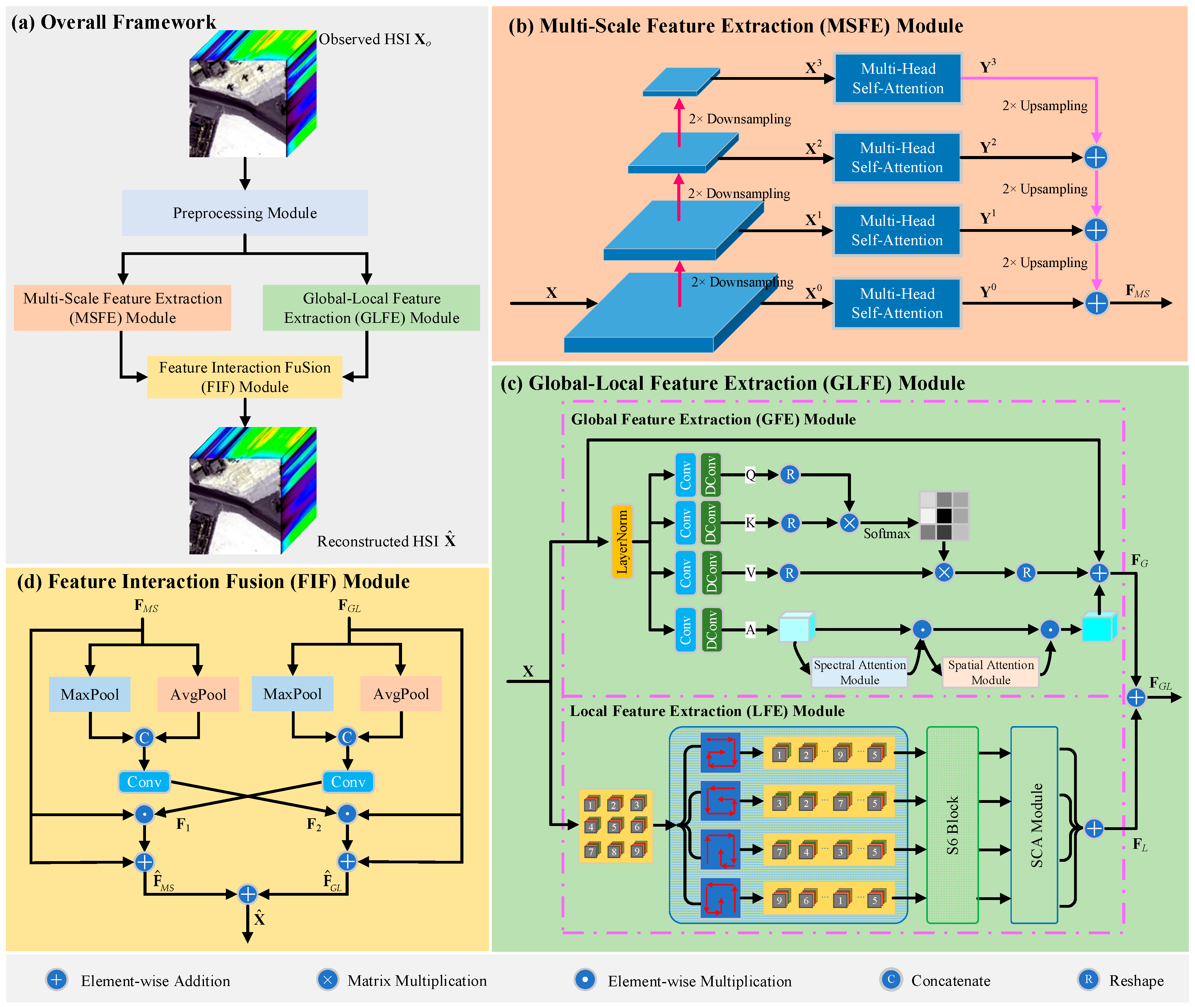
Figure 1. Overall framework of HTMNet.
Remotesensing 17 03015 g001
Figure 2. Multi-head self-attention module.
Remotesensing 17 03015 g002
Figure 3. Framework of spectral attention module.
Remotesensing 17 03015 g003
Figure 4. Framework of spatial attention module.
Remotesensing 17 03015 g004
Figure 5. Schematic diagram of circular scanning.
Remotesensing 17 03015 g005
Figure 6. Four real HSI datasets used in this article. The first and second rows signify the false-color images and GT maps, respectively.
Remotesensing 17 03015 g006
Figure 7. ROC curve comparisons for various HTD methods on four HSI datasets. The first to fourth columns, respectively, represent the ROC(PF, PD), ROC(τ, PD), ROC(τ, PF), and ROC(τ, PF, PD) curves.
Remotesensing 17 03015 g007
Figure 8. Background-target separation maps of various HTD methods on four HSI datasets.
Remotesensing 17 03015 g008
Figure 9. Visualized results of various HTD methods on four HSI datasets.
Remotesensing 17 03015 g009
Figure 10. (a) SpecTIR dataset. (b) Salinas dataset.
Remotesensing 17 03015 g010
Figure 11. Visualized results of various HTD methods on SpecTIR and Salinas datasets.
Remotesensing 17 03015 g011
Figure 12. Parameter analysis of P and H on four HSI datasets. (a) Impact of the patch size P. (b) Impact of the number of attention heads H.
Remotesensing 17 03015 g012
Table 1. Ablation study results [AUC(PF, PD)] on four HSI datasets.
SSFE (Baseline)MSFEGLFEFIFSan Diego ISan Diego IIAbu-Airport-2Abu-Beach-4
0.99120.99220.99160.9841
0.99860.99800.99510.9867
0.99940.99890.99720.9932
0.99970.99910.99820.9964
Table 2. Comparison of AUC scores and inference time (in seconds) for various HTD methods on four HSI datasets. The best results are indicated in bold, with the second-best underlined; the same is the case below.
DatasetAUC ValuesCEMCTTDTD_TSETSTTDHTD-IRNHTD-MambaOurs
San Diego IAUC(PF, PD) ↑0.81510.69290.93090.99710.99830.99940.9997
AUC(τ, PD) ↑0.35910.55340.03060.72960.56330.93110.8998
AUC(τ, PF) ↓0.25040.31700.00040.00080.00440.00660.0074
AUCODP0.92380.92930.96111.72591.55721.92411.8921
AUCSNPR1.43401.745677.3617974.6511127.0831140.2938121.3924
Inference time ↓0.34100.35600.56202.89002.72621.75621.8530
San Diego IIAUC(PF, PD) ↑0.98650.98690.96950.99780.99670.99860.9991
AUC(τ, PD) ↑0.38680.50530.04990.68040.45000.82800.8435
AUC(τ, PF) ↓0.16680.05250.00110.00150.00320.01720.0057
AUCODP1.20651.43971.01831.67671.44351.80941.8368
AUCSNPR2.31889.630744.6177461.7719140.871148.2789147.2270
Inference time ↓0.42650.32560.42362.65002.86261.76521.8226
Abu-airport-2AUC(PF, PD) ↑0.83610.80360.95110.97450.92500.99680.9982
AUC(τ, PD) ↑0.22300.61240.07730.51540.56330.70510.6043
AUC(τ, PF) ↓0.10430.46690.00060.00630.08520.00900.0052
AUCODP0.95480.94911.02781.48361.40311.69291.5973
AUCSNPR2.13811.3116132.801082.44636.608578.2876116.8085
Inference time ↓0.36590.26520.39522.95562.96521.79661.7952
Abu-beach-4AUC(PF, PD) ↑0.94190.90340.91740.94810.94830.99230.9964
AUC(τ, PD) ↑0.40890.22010.03320.04270.48220.34820.5306
AUC(τ, PF) ↓0.17040.04890.00230.00020.06130.00250.0033
AUCODP1.18041.07460.94830.99071.36921.33801.5237
AUCSNPR2.39884.501814.3010227.30697.8677138.7763161.0973
Inference time ↓0.08960.56240.35622.86543.95212.95352.3655
Table 3. Impact of different fusion modules on four HSI datasets [AUC(PF, PD)].
AdditionCross-AttentionFIFSan Diego ISan Diego IIAbu-Airport-2Abu-Beach-4
0.99940.99890.99720.9932
0.99970.99900.99790.9955
0.99970.99910.99820.9964
Table 4. Comparison of AUC scores for various HTD methods on two HSI datasets.
DatasetAUC ValuesCEMCTTDTD_TSETSTTDHTD-IRNHTD-MambaOurs
SpecTIRAUC(PF, PD) ↑0.74780.93030.98360.99220.85680.99300.9993
AUC(τ, PD) ↑0.37470.39850.11480.52230.64640.60900.6996
AUC(τ, PF) ↓0.12080.02270.00010.00020.01110.00740.0034
AUCODP1.00171.30611.09831.51431.49221.59461.6955
AUCSNPR3.100917.54201116.88572694.816458.093782.7502207.2633
SalinasAUC(PF, PD) ↑0.99540.88490.97740.96950.95240.99840.9994
AUC(τ, PD) ↑0.58210.78810.14640.65120.55710.81860.7809
AUC(τ, PF) ↓0.08930.10220.00150.01040.03660.00080.0002
AUCODP1.48811.57081.12231.61021.47291.81621.7801
AUCSNPR6.51557.713496.782362.342315.2363975.03074207.4922
Table 5. Computational complexity comparison for deep learning-based methods on the San Diego I dataset.
MethodsTSTTDHTD-IRNHTD-MambaHTMNet
Params. (M)0.910.410.341.43
Memory usage (M)895.8774.3890.41057.6
FLOPs (G)1.951.760.222.55
Table 6. Impact of SSA block on four HSI datasets [AUC(PF, PD)].
San Diego ISan Diego IIAbu-Airport-2Abu-Beach-4
w/o SSA0.99890.99840.99600.9911
w/SSA0.99940.99890.99720.9932
Table 7. Impact of similarity on four HSI datasets [AUC(PF, PD)].
San Diego ISan Diego IIAbu-Airport-2Abu-Beach-4
Euclidean distance0.99950.99890.99780.9962
Cosine similarity0.99970.99910.99820.9964
Disclaimer/Publisher’s Note: The statements, opinions and data contained in all publications are solely those of the individual author(s) and contributor(s) and not of MDPI and/or the editor(s). MDPI and/or the editor(s) disclaim responsibility for any injury to people or property resulting from any ideas, methods, instructions or products referred to in the content.