A Study of Global Hourly Sea Surface Temperature Fusion Based on the Triple-Collocation Fusion Algorithm

Abstract

Sea surface temperature (SST) is vital for climate monitoring and extreme weather forecasting. Existing global SST datasets are typically provided at daily to seasonal resolutions, while hourly data remain limited to regional scales. Polar-orbiting satellites offer global coverage but low temporal resolution, providing only 1–2 observations per day. Geostationary satellites provide high temporal resolution but cover only part of the region. These limitations create a gap in the availability of global, hourly SST data. To address this, we propose a Triple-Collocation (TC)-based fusion algorithm for generating accurate global hourly SST data through multi-source integration. The method includes data preprocessing (quality control and linear interpolation), merging five geostationary SST datasets into two global sets by priority, applying TC fusion to three polar-orbiting datasets, and finally combining all sources via multi-source TC fusion. Results show improved temporal resolution and increased spatial coverage to 32%. The fused dataset achieves high accuracy, with a daily mean Bias below 0.0427 °C, RMSE about 0.5938 °C to 0.6965 °C, and R² exceeding 0.9879. These outcomes demonstrate the method’s reliability and its potential for supporting climate and environmental research.

1. Introduction

The ocean covers 71% of the Earth’s surface, absorbs the majority of incoming solar radiation, and plays a vital role in atmospheric energy transfer [1]. As the interface for air–sea interactions, variations in the thermal state of the ocean’s surface layer have a significant impact on atmospheric dynamics. SST is the main parameter describing the thermal state of the ocean’s surface layer and is crucial for understanding the marine environment, global climate change, and disaster prevention and mitigation [2]. Accurate, high-coverage SST data are essential for various applications. Traditional methods, such as using ships and buoys, offer high precision but suffer from sparse and uneven spatial distribution [3,4,5]. SST derived from thermal infrared data is often limited by gaps caused by clouds and atmospheric aerosols, resulting in coverage that fails to meet application needs [6]. While microwave sensors can provide full coverage, their spatial resolution is low, and they are sensitive to heavy rainfall [7]. Polar-orbiting satellites provide global SST coverage due to their orbital characteristics and observation times. However, their temporal resolution is limited, typically offering only two observations per day [8]. In contrast, geostationary satellites deliver higher temporal resolution—ranging from one hour to as frequent as every ten minutes—but their spatial coverage is more restricted [9]. Therefore, integrating multi-source SST data is crucial for generating products that combine high spatial and temporal resolution, extensive coverage, and improved accuracy.

Existing studies on global SST analysis are mostly confined to daily, monthly, or seasonal scales, often failing to capture critical information within hourly variations. Seasonal scales can reflect long-term trends, such as monsoon changes. This information is important for the fishing industry [10]. However, it is unable to portray the hourly temperature abruptness of events such as ocean heat waves and typhoon transits; the diurnal variation of SST significantly affects the ocean–atmosphere thermal interactions [11], and the time-by-time data can fill the research gaps of short-term climate processes, such as analyzing the impact of time-by-time variation of SST on the atmospheric circulation during strong storms and improving the accuracy of numerical weather prediction to provide real-time disaster warnings in coastal areas [12]. Therefore, the fusion of multi-source data to build a time-dependent, high-coverage, high-precision SST product can not only make up for the defects of a single data source, but also establish a refined time-series standard for climate research through the integration of time-dependent data, and promote the related fields to real-time dynamic monitoring.

Multi-source data fusion refers to integrating information from different sensors—whether of varying types or from the same sensor at different times—into a unified representation of the same entity [13]. Common data fusion methods include objective analysis, optimal interpolation (OI), and Kalman filtering [14]. Objective analysis, first applied to data fusion in the United States in 1965, has since become a well-established technique for solving practical data fusion challenges. Guan, L. and Kawamura, H. [15] applied objective analysis to fuse SST data from microwave and infrared sensors, resulting in a global SST product with a temporal resolution of one day and a spatial resolution of 25 km. OI introduced by Eliassen in 1954, as part of objective analysis methods, was employed by Reynolds, R.W. et al. [16] to combine AVHRR SST data with observational SST data, producing a fused product with a temporal resolution of one day and a spatial resolution of 0.25°. Additionally, Li, Y. et al. [17] used data interpolation empirical orthogonal function (DINEOF) alongside the OI method to successfully fuse microwave and infrared SST data in the Arctic region. Kalman filtering, first introduced to meteorology and oceanography by Michael, G. and Malanotte-Rizzoli, P., iteratively calculates optimal Kalman coefficients to provide the best estimate of a system’s state [18]. Xi, M. [19] applied OI to fuse infrared (AVHRR) and microwave (AMSR-E) SST data in the mid-latitude southern Indian Ocean, producing a high-resolution SST product that successfully captured the structure of oceanic fronts. One of the key advantages of Kalman filtering over optimal interpolation is its ability to enhance spatial coverage while preserving more detailed information, making it a more effective tool for SST data fusion. Wang, Y. [20] also used AVHRR and AMSR-E SST data, exploring the application of Kalman filtering in SST fusion. In 2008, Ding, R. [21] developed an SST product with a 1-day temporal resolution and approximately 2 km spatial resolution. He applied optimal interpolation and Bayesian maximum entropy methods to fuse SST data from MODIS infrared, AMSR-2, and HY-2A microwave radiometers. In contrast, Liao, Z. [22] focused on SST data from the FY-3C satellite, using both optimal interpolation and Kalman filtering methods for data fusion. He further employed the radial basis function network (RBFN) to enhance the representation of SST details in the fused results. Additionally, Wang, M. et al. [23] achieved multi-source fusion of conventional observations, satellite data, and 3D analysis using a deep learning-based ocean data fusion network (ODF network).

The TC fusion algorithm presented in this paper extends the Triple-Collocation method, first introduced in 1998 [24]. The TC algorithm is widely used for evaluating and analyzing data from multiple sources [25]. It operates by using three independent datasets, each containing observations of the same geophysical variable but differing in error characteristics. By comparing discrepancies among these datasets, the error variance of each can be estimated [26]. Christoforos, T. [27] conducted a study comparing four TC algorithms using buoy-reported real SST, ATSRs/SST, and AMSR-E/SST data. He also determined the minimum sample size required for analysis. Xu, F. et al. [28] applied the TC algorithm to assess SSTs from major platforms in the NOAA In Situ Quality Monitoring (iQuam) system, using data from NOAA-17 AVHRR and Envisat AATSR, both produced by ESA under the Climate Change Initiative (CCI) program. The study revealed the standard deviations of SST errors for various platforms as analyzed using the TC algorithm. For ships, the error was 0.75 K, while for buoys and Argo floats, it ranged from 0.21 to 0.22 K. Tropical moorings showed an error of 0.17 K, and coastal moorings had an error of 0.40 K. The errors for AVHRR and AATSR were between 0.35–0.38 K and 0.15–0.30 K, respectively.

Li, C. et al. [29] assessed the applicability of multi-source precipitation products in China from 2013 to 2015 using the TC algorithm. Their results showed a relative Bias of 4.5% in the southern region and a root mean square error (RMSE) of 0.61 for the Tibetan Plateau. These findings indicate that the TC algorithm provides reliable precipitation estimates for China. Wang, S. et al. [30] applied the TC algorithm to fuse three independent soil moisture products at two spatial scales in the Nagqu region, demonstrating that the fused data were more comprehensive and accurate. Zhou, L. et al. [31] utilized surface temperature products from FY-3C/VIRR, MODIS, and ground observations for multi-source fusion in the Huaihe River Basin. In summary, while the TC algorithm has been widely applied to SST analysis, precipitation evaluation, and soil moisture fusion, no research has yet focused specifically on the fusion of multi-source SST data using this algorithm.

This paper presents a novel approach to SST fusion using the TC fusion algorithm, effectively integrating multi-source SST data from both polar-orbiting and geostationary satellites. This fusion enhances global SST spatial coverage and increases temporal resolution from twice daily to hourly intervals. The performance of the resulting global temporal SST product is evaluated based on key metrics, including spatial coverage, Bias relative to measured data, RMSE, and R².

2. Data Presentation

The accuracy and diversity of SST data are essential for achieving high-precision data fusion. This study uses heterogeneous data from multiple sources, including polar-orbiting satellites, geostationary satellites, and measured data, to ensure comprehensive spatial and temporal coverage. However, due to satellite orbit limitations and sea ice, effective data are concentrated in mid-latitude and low-latitude sea areas and coastal regions, with less coverage in polar regions [32]. The technical parameters of each data source are detailed in the next section. Polar-orbiting satellite data provide the foundational global coverage, while geostationary satellites offer high-frequency observations at mid and low latitudes. Measured data are used for calibration and validation. By organizing the temporal resolution, spatial resolution, data level, and coverage of each source, a solid foundation is laid for applying the TC fusion algorithm and analyzing the results.

2.1. Polar-Orbiting Satellite Data

The polar-orbiting satellite data used in this study include global SST products from AMSR2, MODIS, and AVHRR.

AMSR2 (Advanced Microwave Scanning Radiometer 2) is onboard the GCOM-W1 satellite, developed by the Japan Aerospace Exploration Agency (JAXA), Tsukuba, Japan. It is designed to detect microwave radiation signals from the Earth’s surface and atmosphere [33]. The data used here are high-resolution sea surface temperature (GHRSST) products, specifically fusion-processed daily L3-level data, covering the global ocean from 1 to 2 September 2023. The spatial resolution is 0.25°, with coverage extending from 89.875°N to 89.875°S and from −179.875° to 179.875° longitude, providing near-global ocean coverage, with the exception of small polar regions.

The Moderate Resolution Imaging Spectroradiometer (MODIS, National Aeronautics and Space Administration (NASA), Washington, DC, USA) is a key instrument for observing global biological and physical processes, providing twice-daily observations across 16 thermal infrared bands [34]. The MODIS SST data used in this study have a temporal resolution of twice per day, a spatial resolution of 4 km, and cover the period from 1 to 2 September 2023, matching the AMSR2 data. The coverage spans from 90°N to 90°S latitude and 180°E to 180°W longitude, providing comprehensive global ocean coverage.

The Advanced Very High Resolution Radiometer (AVHRR, National Oceanic and Atmospheric Administration (NOAA), Washington, DC, USA) is a multi-spectral channel scanning radiometer, playing a crucial role in global ocean research and meteorological monitoring applications [35]. The SST data used in this study are derived from the AVHRR thermal infrared band, based on L3 level datasets compiled by GHRSST. These data have a temporal resolution of twice per day, a spatial resolution of 0.05°, and cover the period from 1 to 2 September 2023. The coverage spans from 90°N to 90°S latitude and 180°E to 180°W longitude, ensuring full global ocean coverage.

2.2. Geostationary Satellite Data

The specific temporal resolution, spatial resolution, data level, and spatial coverage of the geostationary satellite SST data used in this paper are summarized in

Table 1. Information on geostationary satellite sea surface temperature data products.

Data	Spatial Resolution	Spatial Extent
		Longitude	Latitude
Himawari-9 SST	2 km	180°W~160°W and 80°E~180°E	60°S~60°N
Met10_SEVIRI SST	5 km	60°W~60°E	60°S~60°N
Met09_SEVIRI SST	3 km	18.5°W~101.5°E	60°S~60°N
G16_ABI SST	2 km	135°W~15°W	60°S~60°N
G18_ABI SST	2 km	and 180°W~77°W 163°E~180°E	60°S~60°N

.

Himawari-9, launched in March 2017, is equipped with a hyperspectral imager (AHI) featuring 16 observation bands [36]. The satellite provides full-disc observations every 10 min. The SST data used in this study are L3C-class products, aggregated from these 10 min intervals to achieve a temporal resolution of 1 h and a spatial resolution of 2 km. The data cover latitudes from 60°S to 60°N and longitudes from 180°W to 160°E and 80°E to 180°E.

Meteosat, operated by the European Organisation for the Exploitation of Meteorological Satellites (EUMETSAT), offers SST data from the Meteosat-9 (Met09/SST) and Meteosat-10 (Met10/SST) satellites. Met09/SST covers the Indian Ocean, with a latitudinal range of 60°S to 60°N and longitudinal range of 101.5°E to 18.5°W. It provides L3C-level SST data on a 0.05° grid, aggregated from 15 min interval data to create 1 h temporal resolution products. Met10_SEVIRI, which covers the eastern Atlantic, also provides high-resolution SST data, remapped to a regular grid with 1 h temporal resolution.

The GOES satellites, operated by NOAA, continuously monitor Earth’s atmosphere, oceans, and surface, providing ocean surface temperature measurements that are processed by ACSPO to generate SST data. This paper uses SST data from G16-ABI and G18-ABI. G16-ABI has a temporal resolution of 1 h, with 0.2 GB of daily data, covering 59°S to 59°N and 135°W to 15°W at a 2 km resolution. G18-ABI also has 1 h temporal resolution, with 0.7 GB of daily data, covering 60°S to 60°N and 180°W to 77°W/163°E to 180°E, also at 2 km resolution.

2.3. Measured Data

The iQuam product, developed by NOAA’s Satellite Applications and Research Center (STAR), integrates buoy, ship, and other survey data for SST analysis [3]. The data are archived monthly, with updates every 12 h and a 2 h delay. All data processing for the previous month is completed by the 15th of the following month. The system performs three primary functions in near real time: quality control (QC) of field SST, online monitoring of field SST after QC, and the provision of reformatted field SST data with quality grades and flags. The data are stored in point form and is available for download at http://www.star.nesdis.noaa.gov/sod/sst/iquam/index.html (accessed on 20 November 2023).

3. Methods

In this paper, we apply the TC algorithm proposed by Tan, S. et al. [26] to SST data fusion for the first time, offering an innovative solution for high-precision global SST fusion. The TC fusion algorithm consists of two steps: First, the error variance of various datasets is estimated using the TC algorithm. Second, fusion weights for the data are determined based on the estimated error variance, followed by the data fusion process. The TC algorithm relies on four assumptions:

(1)

The three SST products are linearly correlated with the true value;

(2)

The errors of the three SST products do not vary with time;

(3)

The errors of the three SST products are independent of each other, i.e., the covariance between the errors of different products is zero;

(4)

The errors of the three SST products are independent of each other and of the true value, i.e., the covariance between the errors of the three products and the true value is 0.

Based on the four assumptions, the relational equations for the three different data values are established as shown below:

$$\left\{\begin{array}{c}{\mathit{T}}_{\mathit{x}}={\alpha }_{\mathit{x}}+{\beta }_{\mathit{x}} {\mathit{T}}_{\mathit{t}}+{\epsilon }_{\mathit{x}}\\ {\mathit{T}}_{\mathit{y}}={\alpha }_{\mathit{y}}+{\beta }_{\mathit{y}} {\mathit{T}}_{\mathit{t}}+{\epsilon }_{\mathit{y}}\\ {\mathit{T}}_{\mathit{z}}={\alpha }_{\mathit{z}}+{\beta }_{\mathit{z}} {\mathit{T}}_{\mathit{t}}+{\epsilon }_{\mathit{z}}\end{array},\right.$$

(1)

where ${\mathit{T}}_{\mathit{x}}, {\mathit{T}}_{\mathit{y}}, {\mathit{T}}_{\mathit{z}}$ are the three data values corresponding to the same image element; ${\mathit{T}}_{\mathit{t}}$ is the true value of the SST; ${\alpha }_{\mathit{x}}, {\alpha }_{\mathit{y}}, {\alpha }_{\mathit{z}}$ are the additive deviation coefficients of the three SST products ${\mathit{T}}_{\mathit{x}}, {\mathit{T}}_{\mathit{y}}, {\mathit{T}}_{\mathit{z}}$ relative to the true value of the SST ${\mathit{T}}_{\mathit{t}}$; ${\beta }_{\mathit{x}}, {\beta }_{\mathit{y}}, {\beta }_{\mathit{z}}$ are the multiplicative deviation coefficients of the three SST products ${\mathit{T}}_{\mathit{x}}, {\mathit{T}}_{\mathit{y}}, {\mathit{T}}_{\mathit{z}}$ relative to the true value of the SST ${\mathit{T}}_{\mathit{t}}$; ${\epsilon }_{\mathit{x}}, {\epsilon }_{\mathit{y}}, {\epsilon }_{\mathit{z}}$ are the errors that the mean of the three SST products is 0, respectively. Any of the data in ${\mathit{T}}_{\mathit{x}}, {\mathit{T}}_{\mathit{y}}, {\mathit{T}}_{\mathit{z}}$ are selected as a reference sample, and in this paper, the data of ${\mathit{T}}_{\mathit{x}}$ are selected as a reference sample to construct the scaling coefficients ${\beta }_{\mathit{y}}^{*}$, ${\beta }_{\mathit{Z}}^{*}$, and 2 new sequences ${\mathit{T}}_{\mathit{y}}^{*}, {\mathit{T}}_{\mathit{Z}}^{*}$:

$$\left\{\begin{array}{c}{\beta }_{\mathit{y}}^{*}={\displaystyle \frac{<{(\mathit{T}}_{\mathit{x}}-\overline{{\mathit{T}}_{\mathit{x}}})\left({\mathit{T}}_{\mathit{z}}-\overline{{\mathit{T}}_{\mathit{z}}}\right)>}{<{(\mathit{T}}_{\mathit{y}}-{\mathit{T}}_{\mathit{y}})\left({\mathit{T}}_{\mathit{z}}-{\mathit{T}}_{\mathit{z}}\right)>}}\\ {\beta }_{\mathit{z}}^{*}={\displaystyle \frac{<({\mathit{T}}_{\mathit{x}}-\overline{{\mathit{T}}_{\mathit{x}}})\left({\mathit{T}}_{\mathit{y}}-\overline{{\mathit{T}}_{\mathit{y}}}\right)>}{<({\mathit{T}}_{\mathit{y}}-{\mathit{T}}_{\mathit{y}})\left({\mathit{T}}_{\mathit{z}}-{\mathit{T}}_{\mathit{z}}\right)>}}\end{array},\right.$$

(2)

$$\left\{\begin{array}{c}{\mathit{T}}_{\mathit{y}}^{*}={\beta }_{\mathit{y}}^{*}\left({\mathit{T}}_{\mathit{y}}-\overline{{\mathit{T}}_{\mathit{y}}}\right)+\overline{{\mathit{T}}_{\mathit{x}}}\\ {\mathit{T}}_{\mathit{z}}^{*}={\beta }_{\mathit{Z}}^{*}\left({\mathit{T}}_{\mathit{Z}}-\overline{{\mathit{T}}_{\mathit{Z}}}\right)+\overline{{\mathit{T}}_{\mathit{x}}}\end{array},\right.$$

(3)

where: $<(*)\left(*\right)>$ is the mean value calculated by multiplying the corresponding elements of the 2 sets of samples two by two. The construction of the scaling factor ${\beta }_{\mathit{y}}^{*}$, ${\beta }_{\mathit{Z}}^{*}$ utilizes the 2 irrelevance assumptions (Assumption (3) and Assumption (4)), so that on the one hand, it can be derived directly by the operation between the two samples, for a definite value; on the other hand, it can be reduced to the ratio of the coefficients of deviation of the linear multiplication of the two samples. For example, it can be obtained from E() = 0:

$${\mathit{T}}_{\mathit{i}}-\stackrel{\mathit{-}}{{\mathit{T}}_{\mathit{j}}}=({\alpha }_{\mathit{i}}+{\beta }_{\mathit{i}}{\mathit{T}}_{\mathit{t}}+{\epsilon }_{\mathit{i}})-({\alpha }_{\mathit{i}}+{\beta }_{\mathit{i}}{\mathit{T}}_{\mathit{t}})={\beta }_{\mathit{i}}\left({\mathit{T}}_{\mathit{t}}-\overline{{\mathit{T}}_{\mathit{t}}}\right)+{\epsilon }_{\mathit{i}},$$

(4)

Substituting Equation (4) into Equation (2) and eliminating the term with zero according to Assumption (3) and Assumption (4) yields:

$$\begin{array}{}{\beta }_{\mathit{y}}^{*}={\displaystyle \frac{<{(\mathit{T}}_{\mathit{x}}-\overline{{\mathit{T}}_{\mathit{x}}})\left({\mathit{T}}_{\mathit{z}}-\overline{{\mathit{T}}_{\mathit{z}}}\right)>}{<{(\mathit{T}}_{\mathit{y}}-{\mathit{T}}_{\mathit{y}})\left({\mathit{T}}_{\mathit{z}}-{\mathit{T}}_{\mathit{z}}\right)>}}= {\displaystyle \frac{{\beta }_{\mathit{x}}{\beta }_{\mathit{z}}<{{(\mathit{T}}_{\mathit{t}}-\overline{{\mathit{T}}_{\mathit{t}}})}^2>+{\beta }_{\mathit{x}}<\left({\mathit{T}}_{\mathit{t}}-\overline{{\mathit{T}}_{\mathit{t}}}\right){\epsilon }_{\mathit{z}}>+{\beta }_{\mathit{z}}<\left({\mathit{T}}_{\mathit{t}}-\overline{{\mathit{T}}_{\mathit{t}}}\right){\epsilon }_{\mathit{x}}>+<{\epsilon }_{\mathit{x}}{\epsilon }_{\mathit{z}}>}{{\beta }_{\mathit{y}}{\beta }_{\mathit{z}}<{{(\mathit{T}}_{\mathit{t}}-\overline{{\mathit{T}}_{\mathit{t}}})}^2>+{\beta }_{\mathit{y}}<\left({\mathit{T}}_{\mathit{t}}-\overline{{\mathit{T}}_{\mathit{t}}}\right){\epsilon }_{\mathit{z}}>+{\beta }_{\mathit{z}}<\left({\mathit{T}}_{\mathit{t}}-\overline{{\mathit{T}}_{\mathit{t}}}\right){\epsilon }_{\mathit{y}}>+<{\epsilon }_{\mathit{y}}{\epsilon }_{\mathit{z}}>}}= {\displaystyle \frac{{\beta }_{\mathit{x}}{\beta }_{\mathit{z}}<{{(\mathit{T}}_{\mathit{t}}-\overline{{\mathit{T}}_{\mathit{t}}})}^2>}{{\beta }_{\mathit{y}}{\beta }_{\mathit{z}}<{{(\mathit{T}}_{\mathit{t}}-\overline{{\mathit{T}}_{\mathit{t}}})}^2>}}={\displaystyle \frac{{\beta }_{\mathit{x}}}{{\beta }_{\mathit{y}}}},\end{array}$$

(5)

The same reasoning gives: ${\beta }_{\mathit{z}}^{*}$:

$$\begin{array}{}{\beta }_{\mathit{z}}^{*}={\displaystyle \frac{<{(\mathit{T}}_{\mathit{x}}-\overline{{\mathit{T}}_{\mathit{x}}})\left({\mathit{T}}_{\mathit{y}}-\overline{{\mathit{T}}_{\mathit{y}}}\right)>}{<{(\mathit{T}}_{\mathit{z}}-\overline{{\mathit{T}}_{\mathit{z}}})\left({\mathit{T}}_{\mathit{y}}-\overline{{\mathit{T}}_{\mathit{y}}}\right)>}}= {\displaystyle \frac{{\beta }_{\mathit{x}}{\beta }_{\mathit{y}}<{{(\mathit{T}}_{\mathit{t}}-\overline{{\mathit{T}}_{\mathit{t}}})}^2>+{\beta }_{\mathit{x}}<\left({\mathit{T}}_{\mathit{t}}-\overline{{\mathit{T}}_{\mathit{t}}}\right){\epsilon }_{\mathit{z}}>+{\beta }_{\mathit{y}}<\left({\mathit{T}}_{\mathit{t}}-\overline{{\mathit{T}}_{\mathit{t}}}\right){\epsilon }_{\mathit{x}}>+<{\epsilon }_{\mathit{x}}{\epsilon }_{\mathit{y}}>}{{\beta }_{\mathit{y}}{\beta }_{\mathit{z}}<{{(\mathit{T}}_{\mathit{t}}-\overline{{\mathit{T}}_{\mathit{t}}})}^2>+{\beta }_{\mathit{y}}<\left({\mathit{T}}_{\mathit{t}}-\overline{{\mathit{T}}_{\mathit{t}}}\right){\epsilon }_{\mathit{z}}>+{\beta }_{\mathit{z}}<\left({\mathit{T}}_{\mathit{t}}-\overline{{\mathit{T}}_{\mathit{t}}}\right){\epsilon }_{\mathit{x}}>+<{\epsilon }_{\mathit{x}}{\epsilon }_{\mathit{z}}>}}= {\displaystyle \frac{{\beta }_{\mathit{x}}{\beta }_{\mathit{y}}<{{(\mathit{T}}_{\mathit{t}}-\overline{{\mathit{T}}_{\mathit{t}}})}^2>}{{\beta }_{\mathit{y}}{\beta }_{\mathit{z}}<{{(\mathit{T}}_{\mathit{t}}-\overline{{\mathit{T}}_{\mathit{t}}})}^2>}}={\displaystyle \frac{{\beta }_{\mathit{x}}}{{\beta }_{\mathit{z}}}},\end{array}$$

(6)

Since Equations (5) and (6) with Assumptions (3) and (4), the new sequence ${\mathit{T}}_{\mathit{y}}^{*}, {\mathit{T}}_{\mathit{Z}}^{*}$ in which all ${\alpha }_{\mathit{y}}, {\alpha }_{\mathit{z}}, {\beta }_{\mathit{y}}, {\beta }_{\mathit{z}}$ are transformed into ${\alpha }_{\mathit{x}}, {\beta }_{\mathit{x}}$:

$$\left\{\begin{array}{c}{\mathit{T}}_{\mathit{x}}={\alpha }_{\mathit{x}}+{\beta }_{\mathit{x}} {\mathit{T}}_{\mathit{t}}+{\epsilon }_{\mathit{x}}\\ {\mathit{T}}_{\mathit{y}}^{*}={\alpha }_{\mathit{x}}+{\beta }_{\mathit{x}} {\mathit{T}}_{\mathit{t}}+{{\beta }_{\mathit{y}}^{*}\epsilon }_{\mathit{y}}\\ {\mathit{T}}_{\mathit{Z}}^{*}={\alpha }_{\mathit{x}}+{\beta }_{\mathit{x}} {\mathit{T}}_{\mathit{t}}+{{\beta }_{\mathit{z}}^{*}\epsilon }_{\mathit{z}}\end{array}\right.,$$

(7)

As a result, the term containing the “truth value ${\mathit{T}}_{\mathit{t}}$” can be eliminated by subtracting two by two:

$$\left\{\begin{array}{c}{\mathit{T}}_{\mathit{x}}-{\mathit{T}}_{\mathit{y}}^{*}={\epsilon }_{\mathit{x}}-{{\beta }_{\mathit{y}}^{*}\epsilon }_{\mathit{y}}\\ {\mathit{T}}_{\mathit{x}}-{\mathit{T}}_{\mathit{z}}^{*}={\epsilon }_{\mathit{x}}-{{\beta }_{\mathit{z}}^{*}\epsilon }_{\mathit{z}}\\ {\mathit{T}}_{\mathit{z}}^{*}-{\mathit{T}}_{\mathit{y}}^{*}={{\beta }_{\mathit{z}}^{*}\epsilon }_{\mathit{z}}-{{\beta }_{\mathit{y}}^{*}\epsilon }_{\mathit{y}}\end{array},\right.$$

(8)

According to the 2 irrelevance assumptions (Assumption (3) and Assumption (4)), it follows that

$$\left\{\begin{array}{c}{<(\mathit{T}}_{\mathit{x}}-{\mathit{T}}_{\mathit{y}}^{*}\left)\right({\mathit{T}}_{\mathit{x}}-{\mathit{T}}_{\mathit{z}}^{*})>={<\epsilon }_{\mathit{x}}{\epsilon }_{\mathit{x}}>\\ {<(\mathit{T}}_{\mathit{x}}-{\mathit{T}}_{\mathit{y}}^{*}\left)\right({\mathit{T}}_{\mathit{z}}^{*}-{\mathit{T}}_{\mathit{y}}^{*})>={{\beta }_{\mathit{y}}^{*}}^2{<\epsilon }_{\mathit{y}}{\epsilon }_{\mathit{y}}>\\ <({\mathit{T}}_{\mathit{z}}^{*}-{\mathit{T}}_{\mathit{x}})({\mathit{T}}_{\mathit{z}}^{*}-{\mathit{T}}_{\mathit{y}}^{*})>={{\beta }_{\mathit{z}}^{*}}^2{<\epsilon }_{\mathit{z}}{\epsilon }_{\mathit{z}}>\end{array}\right.,$$

(9)

where ${<\epsilon }_{\mathit{i}}{\epsilon }_{\mathit{i}}>$ is the variance of the random variable ${\sigma }_{{\epsilon }_{\mathit{i}}}$, ${\mathit{T}}_{\mathit{x}}, {\mathit{T}}_{\mathit{y}}^{*}, {\mathit{T}}_{\mathit{z}}^{*}, {\beta }_{\mathit{y}}^{*}, {\beta }_z^{*}$ can all be found from the sample ${\mathit{T}}_{\mathit{x}}, {\mathit{T}}_{\mathit{y}}, {\mathit{T}}_{\mathit{z}}$, so it can be expressed as ${\mathit{T}}_{\mathit{x}}, T_y^{*}, {\mathit{T}}_{\mathit{z}}^{*}$, ${\beta }_{\mathit{y}}^{*}$, ${\beta }_{\mathit{z}}^{*}$:

$$\left\{\begin{array}{c}{\sigma }_{{\epsilon }_{\mathit{x}}}^2={<(\mathit{T}}_{\mathit{x}}-{\mathit{T}}_{\mathit{y}}^{*}\left)\right({\mathit{T}}_{\mathit{x}}-{\mathit{T}}_{\mathit{z}}^{*})>\\ {\sigma }_{{\epsilon }_{\mathit{y}}}^2={\displaystyle \frac{{<(\mathit{T}}_{\mathit{x}}-{\mathit{T}}_{\mathit{y}}^{*}\left)\right({\mathit{T}}_{\mathit{z}}^{*}-{\mathit{T}}_{\mathit{y}}^{*})>}{{{\beta }_{\mathit{y}}^{*}}^2}}\\ {\sigma }_{{\epsilon }_{\mathit{z}}}^2={\displaystyle \frac{{<(\mathit{T}}_{\mathit{z}}-{\mathit{T}}_{\mathit{x}}^{*}\left)\right({\mathit{T}}_{\mathit{z}}^{*}-{\mathit{T}}_{\mathit{y}}^{*})>}{{{\beta }_{\mathit{z}}^{*}}^2}}\end{array},\right.$$

(10)

Then, the TC algorithm was used to determine the error variance of the three data values relative to the true value. Subsequently, the fusion weight for each SST product was calculated pixel by pixel, ultimately enabling the fusion of multi-source data. Based on the number of valid data points from the three SST products for the same image element, after temporal and spatial matching, the fusion of these products is categorized into three scenarios:

(1) When valid data exist for all three SST products for the same image element on the same day, the fusion weights for each SST product are calculated separately using Equation (11):

$$\left\{\begin{array}{c}{\mathit{w}}_{\mathit{x}}={\displaystyle \frac{{\sigma }_{{\epsilon }_{\mathit{x}}}^2{\sigma }_{{\epsilon }_{\mathit{z}}}^2}{{\sigma }_{{\epsilon }_{\mathit{x}}}^2{\sigma }_{{\epsilon }_{\mathit{y}}}^2+{\sigma }_{{\epsilon }_{\mathit{x}}}^2{\sigma }_{{\epsilon }_{\mathit{z}}}^2+{\sigma }_{{\epsilon }_{\mathit{y}}}^2{\sigma }_{{\epsilon }_{\mathit{z}}}^2}}\\ {\mathit{w}}_{\mathit{y}}={\displaystyle \frac{{\sigma }_{{\epsilon }_{\mathit{x}}}^2{\sigma }_{{\epsilon }_{\mathit{z}}}^2}{{\sigma }_{{\epsilon }_{\mathit{x}}}^2{\sigma }_{{\epsilon }_{\mathit{y}}}^2+{\sigma }_{{\epsilon }_{\mathit{x}}}^2{\sigma }_{{\epsilon }_{\mathit{z}}}^2+{\sigma }_{{\epsilon }_{\mathit{y}}}^2{\sigma }_{{\epsilon }_{\mathit{z}}}^2}}\\ {\mathit{w}}_{\mathit{z}}={\displaystyle \frac{{\sigma }_{{\epsilon }_{\mathit{x}}}^2{\sigma }_{{\epsilon }_{\mathit{x}}}^2}{{\sigma }_{{\epsilon }_{\mathit{x}}}^2{\sigma }_{{\epsilon }_{\mathit{y}}}^2+{\sigma }_{{\epsilon }_{\mathit{x}}}^2{\sigma }_{{\epsilon }_{\mathit{z}}}^2+{\sigma }_{{\epsilon }_{\mathit{y}}}^2{\sigma }_{{\epsilon }_{\mathit{z}}}^2}}\end{array},\right.$$

(11)

where ${\mathit{w}}_{\mathit{x}}, {\mathit{w}}_{\mathit{x}}, {\mathit{w}}_{\mathit{x}}$ and represent the fusion weights of the three SST products ${\mathit{T}}_{\mathit{x}}, {\mathit{T}}_{\mathit{y}}, {\mathit{T}}_{\mathit{z}}$, respectively; and then use the fusion weights of the three SST products to calculate the fused SST:

$${\mathit{T}}_{\mathit{m}}={\mathit{w}}_{\mathit{x}}{\mathit{T}}_{\mathit{x}}+{\mathit{w}}_{\mathit{y}}{\mathit{T}}_{\mathit{y}}+{\mathit{w}}_{\mathit{z}}{\mathit{T}}_{\mathit{z}},$$

(12)

where ${\mathit{T}}_{\mathit{m}}$ is the post-fusion SST;

(2) When only two SST products exist with valid data for the same image element on the same day, Equation (13) is used to calculate the fusion weights of these two SST products:

$$\left\{\begin{array}{c}{\mathit{w}}_{\mathit{x}}={\displaystyle \frac{{\sigma }_{{\epsilon }_{\mathit{y}}}^2}{{\sigma }_{{\epsilon }_{\mathit{x}}}^2{+\sigma }_{{\epsilon }_{\mathit{y}}}^2}}\\ {\mathit{w}}_{\mathit{y}}={\displaystyle \frac{{\sigma }_{{\epsilon }_{\mathit{x}}}^2}{{\sigma }_{{\epsilon }_{\mathit{x}}}^2+{\sigma }_{{\epsilon }_{\mathit{y}}}^2}}\end{array},\right.$$

(13)

The fused SSTs were calculated using the fused weights of the two SST products:

$${\mathit{T}}_{\mathit{m}}={\mathit{w}}_{\mathit{x}}{\mathit{T}}_{\mathit{x}}+{\mathit{w}}_{\mathit{y}}{\mathit{T}}_{\mathit{y}},$$

(14)

(3) When only one SST product exists with valid data for the same image element on the same day, the SST of that product is directly assigned to the fused SST:

$${\mathit{T}}_{\mathit{m}}={\mathit{T}}_{\mathit{x}},$$

(15)

In this paper, three commonly used evaluation metrics are selected to measure the accuracy of model fusion data: Bias, root mean square error (RMSE), and coefficient of determination (R²). The formulas for each index are as follows:

$$\mathit{Bias}={\displaystyle \frac{1}{\mathit{n}}}{\sum }_{\mathit{i}=1}^{\mathit{n}}\left({\mathit{X}}_{\mathit{i}}-{\mathit{Y}}_{\mathit{i}}\right),$$

(16)

$$\mathit{RMSE}=\sqrt{{\displaystyle \frac{1}{\mathit{n}}}{\sum }_{\mathit{i}=1}^{\mathit{n}}{\left({\mathit{X}}_{\mathit{i}}-{\mathit{Y}}_{\mathit{i}}\right)}^2},$$

(17)

$${\mathit{R}}^2=1-{\displaystyle \frac{{\sum }_{\mathit{i}=1}^{\mathit{n}}{\left({\mathit{Y}}_{\mathit{i}}-{\mathit{X}}_{\mathit{i}}\right)}^2}{{\sum }_{\mathit{i}=1}^{\mathit{n}}{\left({\mathit{X}}_{\mathit{i}}-\overline{{\mathit{X}}_{\mathit{i}}}\right)}^2}},$$

(18)

where $\mathit{n}$ is the number of samples, $\mathit{Y}$ represents the fusion result data, and $\mathit{X}$ represents the actual measurement obtained from buoys, ships, etc. The smaller the values of the Bias and RMSE indicators, the closer they are to indicating that the fusion of SST data is good and the overall accuracy is higher. Conversely, larger values indicate that the fusion data effect is poor and the accuracy is low.

4. Experiments and Results

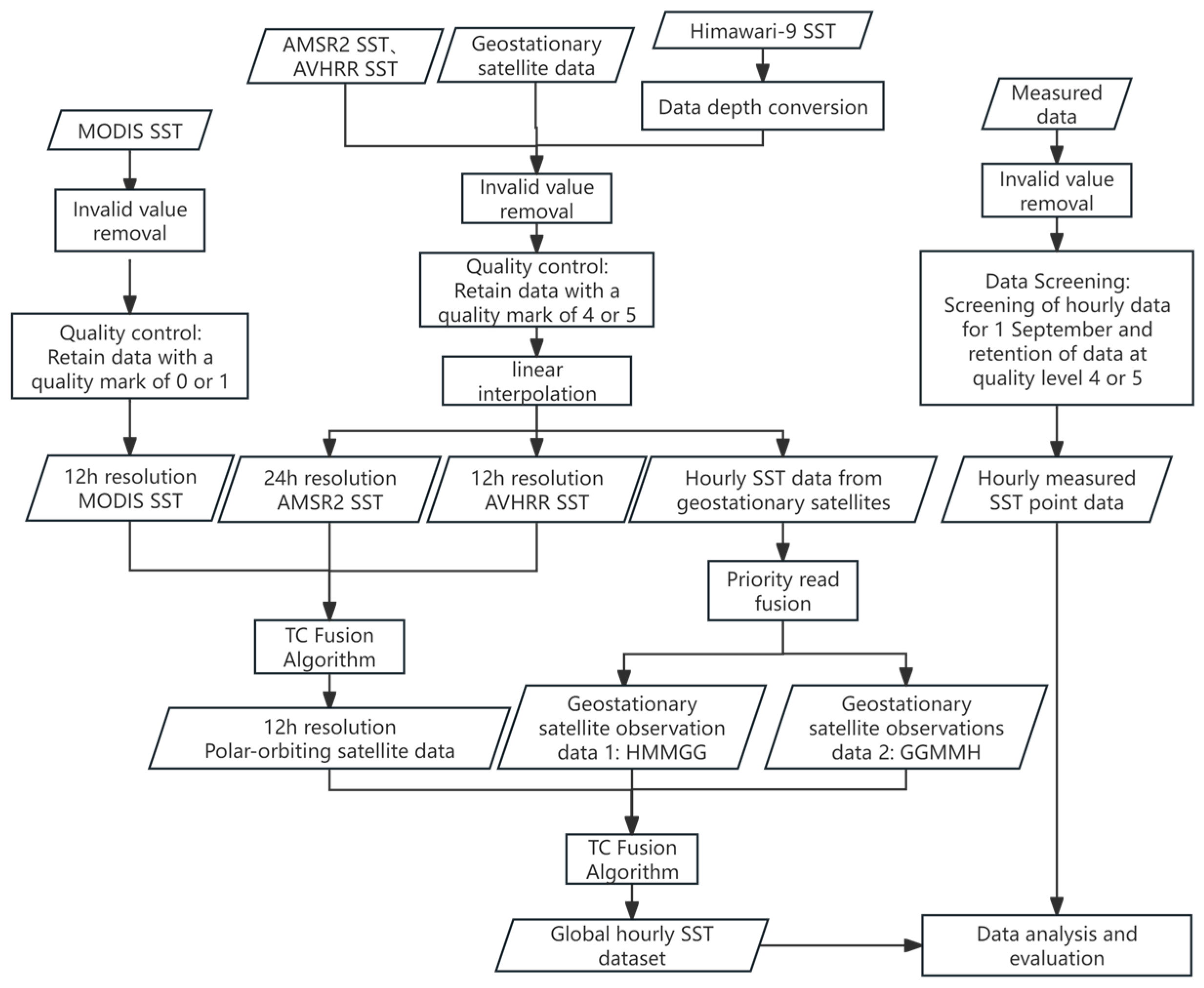
The experimental flow in this paper, shown in Figure 1, covers three core aspects: data preprocessing, fusion experiment, and data evaluation, outlining the complete process from raw data processing to result verification.

4.1. Preprocessing

To ensure the quality and reliability of each SST product and facilitate comparison on the same spatial scale, this paper performs thorough preprocessing before data fusion. The main preprocessing steps include data deep conversion, removing invalid values, quality control, and linear interpolation, which lay the foundation for the subsequent fusion analysis.

During the data preprocessing stage, this study first standardized the measurement depths of the data. As indicated by the fundamental information accompanying the datasets, while the Himawari-9 SST data were measured at the skin depth, all other datasets used in this study were measured at the subskin depth. To achieve depth consistency, we employed the physical conversion model to adjust the Himawari-9 SST data to the subskin level:

$${\mathit{T}}_{\mathit{subskin}}={\mathit{T}}_{\mathit{skin}}- ∆\mathit{T}={\mathit{T}}_{\mathit{skin}}- \mathit{a}(1-e^{-b{U}_{10}})$$

(19)

Key parameters: $\mathit{a}$ $=$ −0.15 (maximum temperature difference coefficient), $b$ = 0.3 (wind speed response coefficient); ${\mathrm{U}}_{10}$ is the 10-m wind speed.

The conversion was applied only to the skin depth SST data from Himawari-9. Data from other sources, originally at the subskin depth, were used directly. Consequently, all merged data products were standardized to the subskin depth, ensuring a consistent physical basis for the fused dataset.

Subsequently, invalid values were removed. This study eliminates the infinity values and NAN invalid values in the data to eliminate the interference of abnormal data on the results. Then, the quality control of the data is carried out on this basis. According to the data description information in the data download webpage, the quality of AMSR2, AVHRR, and the geostationary satellite SST data used are labelled on a scale from 0 to 5, where 0 represents no data, 1 represents data that should not be used in any case due to the influence of clouds, rain, etc., 2 is the worst-quality but usable data, and 5 represents the best-quality data, and the quality level increases step by step from 2 to 5 in a stepwise manner. SST data with quality levels 4 and 5 were selected for this paper based on a combination of data quality and quantity. For the MODIS SST product, the data quality identification also adopts the level from 0 to 5, but the order of good and bad quality is reversed from AMSR2. Therefore, SST data with quality levels 0 and 1 were selected for this paper. After the above processing, the linear interpolation method is used to unify the data grid, and finally, a standardized preprocessed dataset with a spatial resolution of 4 km is obtained.

In processing the measured data, each file contains SST data for the entire month. During the screening process, hourly SST measurements for 1 September were extracted and evaluated based on their quality identifiers. Only data with quality levels 4 or 5 were selected.

4.2. Experiments

As shown in Figure 1, this study uses a rigorous processing procedure in the fusion of SST data. Although the five sets of geostationary satellite data selected for the study can cover the global sea area at low and middle latitudes, there is spatial overlapping of the data. This study follows a priority strategy, processing data in the order of Himawari-9, Met09_SEVIRI, Met10_SEVIRI, G16_ABI, and G18_ABI to generate the first stationary satellite observation dataset (named HMMGG, which stands for Himawari-9, Met09_SEVIRI, Met10_SEVIRI, G16_ABI, and G18_ABI). Subsequently, by adjusting the data reading priority, the data are re-read in the order of G18_ABI, G16_ABI, Met10_SEVIRI, Met09_SEVIRI, and Himawari-9 to generate the second geostationary satellite observation dataset (named GGMMH, formed by the initials of G18_ABI, G16_ABI, Met10_SEVIRI, Met09_SEVIRI, and Himawari-9). The two datasets, HMMGG and GGMMH, provide complementary geostationary satellite SST data sources for the subsequent multi-source fusion through the differentiated data combination strategy, which effectively improves the data diversity and coverage.

For the fusion of polar-orbiting satellite SST data, we applied the TC fusion algorithm to combine three datasets: AMSR2, AVHRR, and MODIS, resulting in SST data with a 12-h temporal resolution. Given the temporal coverage of polar-orbiting satellites, we processed the data across different time windows, generating three SST datasets centered on 00:00, 12:00, and 24:00 UTC on 1 September, each with a 6 h window before and after the central time point.

Finally, the TC fusion algorithm was used to integrate the polar-orbiting satellite data with two geostationary satellite datasets, producing global time-dependent SST data after processing data from various time periods.

4.3. Results

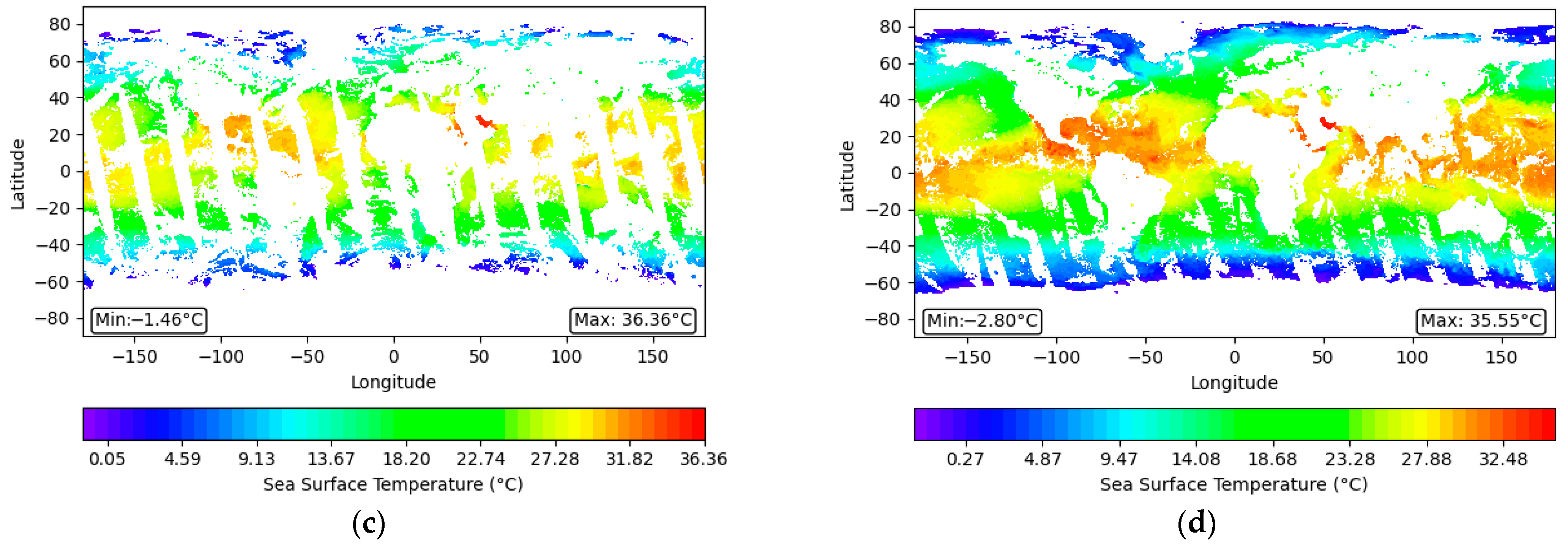
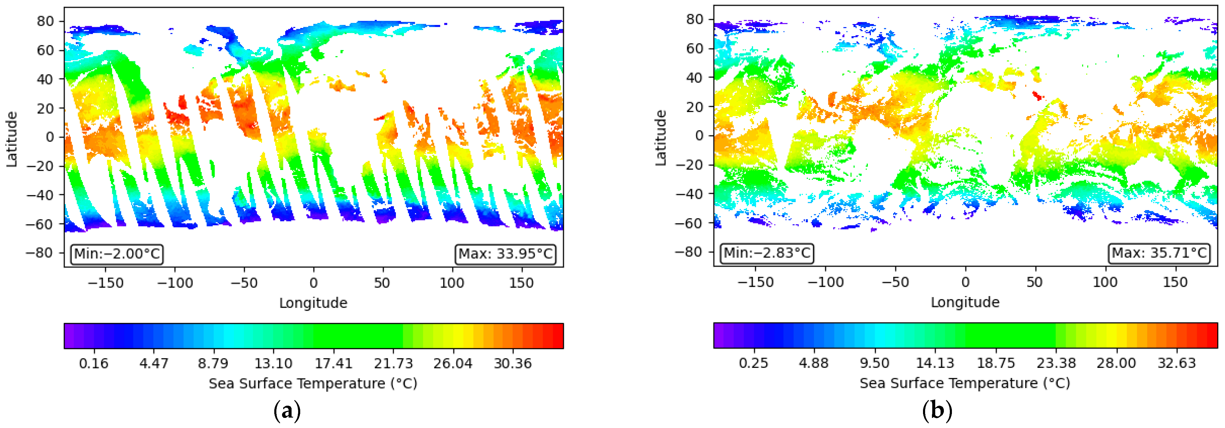
This study uses data from 00:00 UTC on 1 September 2023 as a representative case to visualize the SST data fusion process and stage-wise results. Figure 2a–c display the preprocessed SST images from three types of polar-orbiting satellite data: AMSR2, AVHRR, and MODIS, highlighting the characteristics of the raw data. Figure 2d presents the preliminary results after processing these datasets using the TC fusion algorithm, illustrating the integration of the polar-orbiting satellite data.

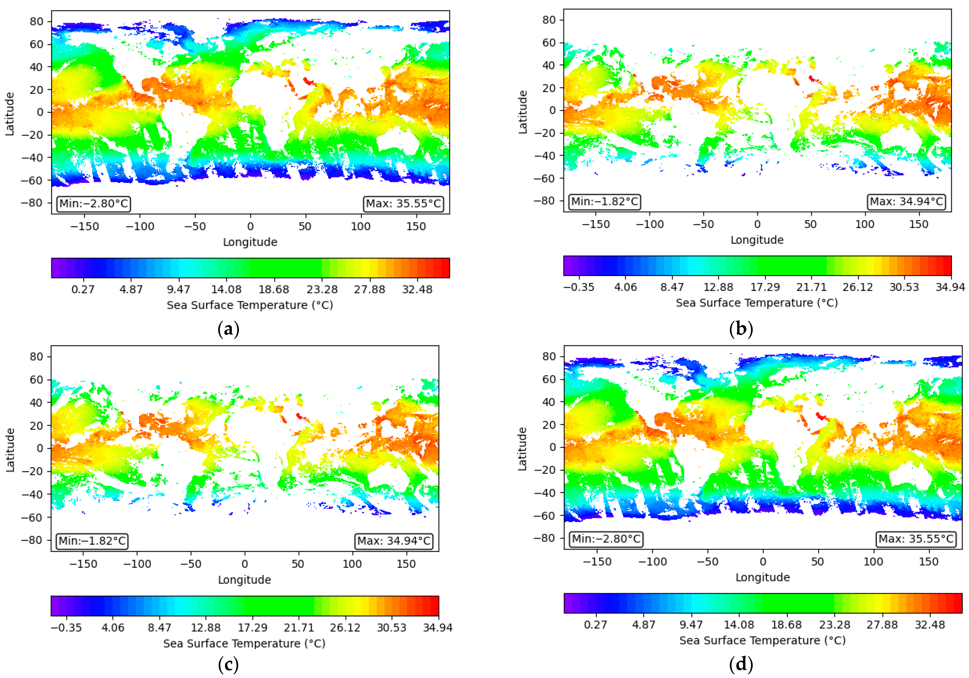
Figure 3 further outlines the subsequent stages of the fusion process. Figure 3a shows the preliminary fusion result of the polar-orbiting satellite data (TC-AAM); Figure 3b,c show the preliminary fusion results of the HMMGG and GGMMH datasets generated from the geostationary satellite data, using different data reading sequences; and Figure 3d shows the final fusion result, TC-AHG, representing the complete global time-series SST data. The two sets of images systematically demonstrate the entire process, from raw data preprocessing and initial fusion of polar-orbiting and geostationary satellite data to the generation of the final global SST dataset.

5. Discussion

In this study, the TC fusion algorithm is applied to both polar-orbiting and geostationary satellite SST data to overcome the spatial and temporal limitations of individual observations. We evaluate its performance in terms of spatial coverage and data accuracy. Specifically, we compare the spatial extent of the fused dataset with that of the original data to quantify improvements in coverage. In addition, we assess data reliability by analyzing deviations from in situ measurements, examining residual distributions, and calculating standard error metrics. The results demonstrate that the TC algorithm significantly enhances both the spatial completeness and the agreement with measured SST values, providing a high-precision foundation for climate research.

5.1. Spatial Coverage Analysis

First, we compare the spatial coverage of the original datasets with that of the fusion results. The SST spatial coverage index in this study is defined as the ratio of valid grid point data to global-scale grid point data. Figure 4a presents the spatial coverage statistics of polar-orbiting satellite data during the TC fusion process. Using the data at 00:00 UTC on 1 September as an example, the AMSR2 dataset—based on microwave measurements—achieves relatively high spatial coverage (25.53%) due to its insensitivity to cloud interference and its 24 h temporal resolution. In contrast, AVHRR and MODIS datasets—derived from thermal infrared measurements—are more affected by cloud cover and have a 12 h temporal resolution, resulting in lower spatial coverage of 14.32% and 9.10%, respectively.

After applying the TC fusion algorithm, the global spatial coverage of SST data increases to 29.89% within the 12 h time window, representing a clear improvement over the original datasets. Figure 4b illustrates the spatial coverage statistics before and after TC fusion at four selected time points: 00:00, 06:00, 12:00, and 18:00 UTC. Notably, the fused polar-orbiting satellite data achieve a spatial coverage of approximately 29%. In contrast, the geostationary satellite data—mainly derived from thermal infrared sensors and concentrated in mid- and low-latitude regions—exhibit lower spatial coverage, remaining around 10%. When combining both polar-orbiting and geostationary satellite data using the TC algorithm, the global spatial coverage of valid SST data further increases to approximately 32%.

5.2. Comparative Analysis with Measured Data

To evaluate the pixel-level deviation between the fused SST data and the in situ measurements, a Cartesian coordinate system is established, where the preprocessed measured SST values are plotted on the x-axis and the fused SST values on the y-axis. The data points are visualized accordingly. As illustrated in Figure 5, the TC fusion results demonstrate a wider distribution of points compared to those from the individual geostationary satellites, yet with very few outliers—indicating a strong overall agreement with the in situ measurements.

Additionally, Figure 6 presents the histograms of residual distributions for the polar-orbiting satellite data, HMMGG data, GGMMH data, and their fused result at 00:00 UTC on 1 September. All residuals approximately follow a normal distribution. Among them, the fused dataset exhibits the smallest mean deviation from the measured values (−0.03 °C). Regarding dispersion, both the fused TC_AHG data and the pre-fusion polar-orbiting data have a standard Bias of 0.70 °C, suggesting similar spread characteristics. In contrast, the geostationary satellite datasets show smaller standard deviations, indicating less variability. Overall, the dispersion of residuals in the final fused dataset is primarily influenced by the polar-orbiting satellite data.

Table 2. Statistics of data accuracy assessment before and after fusion on 1 September 2023 at 00, 06, 12, and 18 moments. It includes the Bias, RMSE, and R² results of TC-AAM, HMMGG, and GGMMH data before fusion and TC-AHG after fusion with respect to the measured SST data at the four moments. The units are in °C.

Time	Data	Bias	RMSE	R2
00	TC_AAM	−0.0894	0.7027	0.9883
	HMMGG	0.0845	0.5685	0.9891
	GGMMH	0.1246	0.5488	0.9901
	TC_AHG	−0.0278	0.6965	0.9879
06	TC_AAM	0.0706	0.6828	0.9890
	HMMGG	−0.0209	0.4937	0.9923
	GGMMH	0.0001	0.4648	0.9932
	TC_AHG	0.0235	0.6471	0.9901
12	TC_AAM	0.0973	0.6075	0.9913
	HMMGG	0.0120	0.5524	0.9924
	GGMMH	0.0180	0.5447	0.9926
	TC_AHG	0.0721	0.6154	0.9909
18	TC_AAM	−0.1348	0.6180	0.9907
	HMMGG	0.1881	0.6394	0.9885
	GGMMH	0.1914	0.6410	0.9887
	TC_AHG	0.0418	0.5938	0.9914

presents the accuracy indexes of the data before and after fusion compared with the measured data at four time points (00:00, 06:00, 12:00, and 18:00) on 1 September 2023. The fused TC-AHG data show outstanding performance in various indexes: the Bias values are −0.0278 °C at 00:00, 0.0235 °C at 06:00, 0.0721 °C at 12:00, and 0.0418 °C at 18:00, with all absolute values less than 0.08 °C, which is significantly better than the pre-fusion data. Specifically, the Bias of TC-AAM ranges from −0.1348 °C to 0.0973 °C, HMMGG from −0.0449 °C to 0.1881 °C, and GGMMH from −0.0275 °C to 0.1914 °C. In particular, at 18:00, the Bias of TC-AHG is 0.0418 °C, which is 79.39%, 77.80%, and 78.20% lower than that of TC-AAM (−0.1348 °C), HMMGG (0.1881 °C), and GGMMH (0.1914 °C), respectively. The RMSE values for TC-AHG range from 0.5938 °C to 0.6965 °C, which is slightly higher than those of HMMGG (0.4648 °C to 0.6394 °C) and GGMMH (0.4648 °C to 0.6410 °C) but combines the advantage of global coverage from polar-orbiting satellites. The coefficients of determination (R²) all exceed 0.9879, reaching 0.9914 at 18:00, indicating an extremely strong correlation between the fused data and the measured data.

Table 3. The following table shows the Bias and RMSE values before and after data fusion for hourly measurements on 1 September 2023. The first six columns present the Bias and RMSE values of the polar-orbiting satellite data (TC-AAM) and two geostationary satellite datasets (HMMGG and GGMMH) relative to the measured data prior to fusion. The last two columns display the Bias and RMSE results of the fused product (TC-AHG) relative to the measured data. All values are in degrees Celsius (°C), with the last row showing the average values.

Time	TC_AAM		HMMGG		GGMMH		TC_AHG
	Bias	RMSE	Bias	RMSE	Bias	RMSE	Bias	RMSE
0	−0.0894	0.7027	0.0845	0.5685	0.1246	0.5488	−0.0278	0.6965
1	−0.0741	0.6946	0.0875	0.5899	0.1048	0.5780	−0.0226	0.7013
2	−0.0510	0.6699	0.0890	0.5988	0.1078	0.5716	−0.0074	0.6590
3	−0.0185	0.6826	0.0285	0.5204	0.0401	0.4972	−0.0029	0.6697
4	0.0078	0.6734	0.0052	0.4723	0.0212	0.4420	−0.0160	0.6510
5	0.0126	0.6870	−0.0449	0.4581	−0.0253	0.4361	−0.0160	0.6466
6	0.0706	0.6828	−0.0209	0.4937	0.0001	0.4648	0.0235	0.6471
7	0.0568	0.6569	−0.0320	0.4925	−0.0069	0.4275	0.0332	0.6245
8	0.0691	0.6356	0.0162	0.4859	0.0095	0.4725	0.0429	0.6199
9	0.0791	0.6146	−0.0260	0.4989	−0.0275	0.4915	0.0438	0.6052
10	0.0942	0.6053	0.0352	0.5514	0.0296	0.5405	0.0830	0.6046
11	0.0983	0.5940	0.0271	0.4994	0.0203	0.4822	0.0686	0.5793
12	0.0973	0.6075	0.0120	0.5524	0.0180	0.5447	0.0721	0.6154
13	0.0832	0.6019	0.0355	0.5461	0.0398	0.5397	0.0701	0.5891
14	0.0630	0.5830	0.0076	0.4999	0.0187	0.4883	0.0454	0.5622
15	0.0403	0.5789	0.0756	0.5392	0.1001	0.5169	0.0503	0.5559
16	−0.0008	0.5823	0.1228	0.5748	0.1513	0.5613	0.0702	0.5870
17	−0.0332	0.6220	0.1713	0.6077	0.1893	0.5953	0.0909	0.5993
18	−0.0779	0.6185	0.1853	0.6048	0.1846	0.5970	0.0719	0.6075
19	−0.1348	0.6180	0.1881	0.6394	0.1914	0.6410	0.0418	0.5938
20	−0.1268	0.6529	0.1812	0.6561	0.2029	0.6459	0.0657	0.6390
21	−0.1295	0.6457	0.1407	0.6484	0.1634	0.6295	0.0350	0.6430
22	−0.1197	0.6396	0.1320	0.6425	0.1574	0.6246	0.0216	0.6264
23	−0.1050	0.6045	0.0397	0.5197	0.0614	0.5044	−0.0021	0.5713
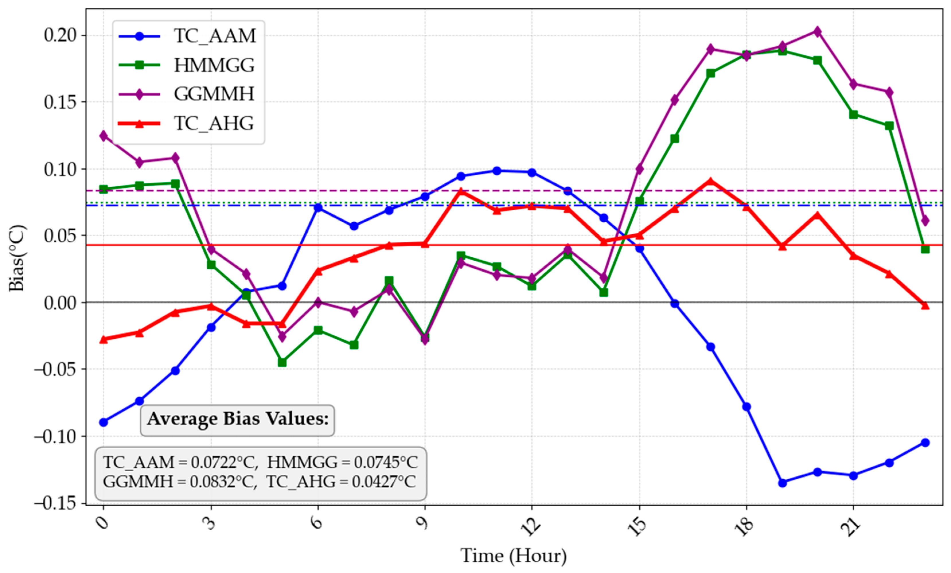
Average	0.0722	0.6356	0.0745	0.5525	0.0832	0.5351	0.0427	0.6206

presents the hourly Bias and RMSE details of data before and after fusion on 1 September 2023 (covering the entire 24 h period). The average Bias of the fused TC-AHG data is 0.042699 °C, which is 40.86%, 42.71%, and 48.66% lower than the pre-fusion TC-AAM (0.072208 °C), HMMGG (0.074532 °C), and GGMMH (0.083167 °C), respectively. RMSE analysis reveals TC-AHG achieves a mean RMSE of 0.6206 °C, 2.36% lower than TC-AAM (0.6356 °C), with its RMSE fluctuation range (0.5713~0.6965 °C) showing 31.4% reduction in standard deviation. The absolute Bias of TC-AHG remains below 0.08 °C during most periods, with minor increases at 10:00 (0.0830 °C) and 17:00 (0.0909 °C) still outperforming pre-fusion data. At 17:00, TC-AAM shows a Bias of −0.0332 °C with an RMSE of 0.6220 °C; HMMGG has a Bias of 0.1713 °C and an RMSE of 0.6077 °C; GGMMH exhibits a Bias of 0.1893 °C and an RMSE of 0.5953 °C; while TC-AHG maintains a Bias of 0.0909 °C and an RMSE of 0.5993 °C. As illustrated in Figure 7, TC-AHG’s Bias fluctuation range (−0.0278 °C to 0.0909 °C) narrows by >52% versus pre-fusion methods (e.g., TC-AAM: −0.1348 °C to 0.0983 °C), with the Bias–RMSE correlation coefficient reduced to 0.62 (TC-AAM: 0.79), indicating simultaneous optimization of systematic and random errors. This enhanced stability provides robust support for hourly scale sea surface temperature monitoring.

In 2021, Li, Y. [17] reconstructed Arctic SST data on an annual scale by fusing multiple data sources. The results showed that the absolute Bias between the fused and in situ measurements ranged from 0.0923 °C to 0.0143 °C, demonstrating a high level of agreement—comparable to the results obtained in this study. In the same year, Zhou, X. [36] conducted hourly SST fusion using Himawari-8 satellite data for the offshore region of China. Their validation results indicated a Bias of 0.09 °C and an RMSE of 0.89 °C. In contrast, the fused SST data presented in this study achieve a global-average Bias of approximately 0.0427 °C and RMSE of 0.6206 °C, values lower than those reported in regional studies such as Zhou et al. (2021) [36]. This further supports the accuracy and robustness of the proposed fusion approach.

The global time-series SST data generated using the TC fusion algorithm in this study not only improves the temporal resolution of SST products but also expands the spatial coverage of individual satellite datasets. Moreover, the fused results show high accuracy and strong consistency with in situ measurements. These findings provide solid evidence for the reliability and effectiveness of the TC fusion algorithm in integrating polar-orbiting and geostationary satellite SST data at a global scale.

6. Conclusions

This study introduces the application of the TC fusion algorithm to effectively integrate SST data from both polar-orbiting and geostationary satellites. A notable advantage of the TC algorithm lies in its ability to autonomously evaluate and fuse multi-source data without the need for prior knowledge. The main objective is to leverage the wide spatial coverage of polar-orbiting satellites and the high temporal resolution of geostationary satellites to generate globally consistent, time-dependent, and high-precision SST datasets. The fused products show clear improvements, notably enhancing the temporal resolution to an hourly scale.

Through careful comparison and analysis of the fusion results with buoy measurement data, we observe that the SST data produced by the TC fusion algorithm demonstrate high accuracy. The spatial coverage of the fused data increased by 6 per cent (32 per cent compared to 26 per cent before fusion) and a daily mean Bias below 0.0427 °C, RMSE from about 0.5938 °C to 0.6965 °C, and R² exceeding 0.9879. These experimental findings robustly confirm the reliability of the TC fusion algorithm in integrating polar-orbiting and geostationary satellite data and showcase the considerable potential of this method for SST data fusion.

This study lays a solid foundation for future research. To enhance practical application value, we plan to integrate the fused SST dataset into numerical weather prediction or climate models to validate its utility in typhoon forecasting and air–sea interaction research. At the methodological level, a key challenge lies in addressing the partial independence limitation of the HMMGG and GGMMH datasets arising from their shared input sources. Concurrently, one of the core priorities for future work is to conduct a comprehensive quantitative comparison to assess the performance of the TC method relative to alternative fusion schemes like Kalman filtering and optimal interpolation. Moreover, to further improve spatial coverage and accuracy—especially in high-latitude regions with limited GEO satellite coverage—future work could integrate VIIRS or other polar-optimized sensors, with careful attention to temporal alignment. These enhancements are expected to further refine the methodology and advance the quality of SST data products.

References

1. Kawai, Y.; Wada, A. Diurnal Sea Surface Temperature Variation and Its Impact on the Atmosphere and Ocean: A Review. J. Oceanogr. 2007, 63, 721–744. [Google Scholar] [CrossRef]
2. Yang, S.; Yan, H. Impact of the north and south ssta in north pacific on rainfall patterns of flood season in China. J. Appl. Meteorol. Sci. 2007, 18, 193–201. [Google Scholar]
3. Xu, F.; Ignatov, A. In situ SST Quality Monitor (iQuam). J. Atmos. Ocean. Technol. 2014, 31, 164–180. [Google Scholar] [CrossRef]
4. Kennedy, J.J.; Rayner, N.A.; Smith, R.O.; Parker, D.E.; Saunby, M. Reassessing biases and other uncertainties in sea surface temperature observations measured in situ since 1850: 2. Biases and homogenization. J. Geophys. Res. 2011, 116, 15220. [Google Scholar] [CrossRef]
5. Stramma, L.; Cornillon, P.; Weller, R.A.; Price, J.F.; Briscoe, M.G. Large Diurnal Sea Surface Temperature Variability: Satellite and In Situ Measurements. J. Phys. Oceanogr. 1986, 16, 827–837. [Google Scholar] [CrossRef]
6. Zhang, C.; Hong, H.; Shang, S. Merging and validation of multi-sensor remote sensing sea surface temperature in the China Sea. In Proceedings of the 2011 International Conference on Remote Sensing, Environment and Transportation Engineering, Nanjing, China, 24–26 June 2011; pp. 4156–4159. [Google Scholar]
7. Guan, L.; Kawamura, H. SST Availabilities of Satellite Infrared and Microwave Measurements. J. Oceanogr. 2003, 59, 201–209. [Google Scholar] [CrossRef]
8. Olafur, J.; Irina, G.; Alexander, I. Towards global daily gridded super-collated SST product from low earth orbiting satellites (L3S-LEO-Daily) at NOAA. In Ocean Sensing and Monitoring XIV, Proceedings of the SPIE Defense + Commercial Sensing, 2022, Orlando, FL, USA, 3–7 April 2022; SPIE: Bellingham, WA, USA, 2022. [Google Scholar]
9. Maturi, E.; Harris, A.; Mittaz, J.; Merchant, C.; Potash, B.; Meng, W.; Sapper, J. NOAA’s Sea Surface Temperature Products from Operational Geostationary Satellites. Bull. Am. Meteorol. Soc. 2008, 89, 1877–1888. [Google Scholar] [CrossRef]
10. Khaled, M.A.; Al-Jamali, F.H.; Said, R.E.; Mohammad, A.S.; Ahmed, M.H.; Ahmed, H.O. Analysis of SST and Chl-a data from MODIS-Aqua in the Major Egyptian Fishing Zones of the Red Sea. Egypt. J. Aquat. Res. 2023, 49, 520–529. [Google Scholar] [CrossRef]
11. Jung, S.; Im, J.; Han, D. PARAN: A novel physics-assisted reconstruction adversarial network using geostationary satellite data to reconstruct hourly sea surface temperatures. Remote Sens. Environ. 2025, 323, 114749. [Google Scholar] [CrossRef]
12. Luo, J. Analysis of Diurnal Variation of Sea Surface Temperature in the South China Sea and Its Influence on Typhoon Simulation. Master’s Thesis, National Marine Environmental Forecasting Center, Beijing, China, 2024. [Google Scholar]
13. Hu, Y.; Zhong, Z.; Liu, X.; Zhu, Y. Influence of air–sea interaction on the simulation of East Asian summer monsoon: A case study. Dyn. Atmos. Ocean. 2012, 53–54, 1–16. [Google Scholar] [CrossRef]
14. Wu, X.; Wang, X.; Li, W.; Han, G.; Zhang, X.; Fu, H.; Li, D. Review of the application of ocean data assimilation and data fusion techniques. J. Ocean. Technol. 2015, 34, 97–103. [Google Scholar]
15. Guan, L.; Kawamura, H. Merging satellite infrared and microwave SSTs: Methodology and evaluation of the new SST. J. Oceanogr. 2004, 60, 905–912. [Google Scholar] [CrossRef]
16. Reynolds, R.W.; Smith, T.M.; Liu, C.; Chelton, D.B.; Casey, K.S.; Schlax, M.G. Daily High-Resolution-Blended Analyses for Sea Surface Temperature. J. Clim. 2007, 20, 5473–5496. [Google Scholar] [CrossRef]
17. Li, Y.; Sun, W.; Zhang, J.; Meng, J.; Zhao, Y. Reconstruction of arctic SST data and generation of multi-source satellite fusion products with high temporal and spatial resolutions. Remote Sens. 2021, 12, 695–703. [Google Scholar] [CrossRef]
18. Michael, G.; Paola, M.-R. Data Assimilation in Meteorology and Oceanography. Adv. Geophys. 1991, 33, 141–266. [Google Scholar] [CrossRef]
19. Xi, M. Merging Infrared Radiometer and Microwave Radiometer Sea Surface Temperature Data Based on the Optimum Interpolation. Master’s Thesis, National Marine Environmental Forecasting Center, Beijing, China, 2011. [Google Scholar]
20. Wang, Y.; Guan, L.; Qu, L. Merging sea surface temperature observed by satellite infrared and microwave radiometers using kalman filter. Period. Ocean. Univ. China 2010, 40, 126–130. [Google Scholar] [CrossRef]
21. Ding, R.; Zhao, C. Study on the merging sea surface temperature data based on optimal interpolation and bayesian maximum entropy method. J. Ocean. Technol. 2018, 37, 35–42. [Google Scholar]
22. Liao, Z. Sea Surface Temperature Reconstruction for fy-3c Satellite Data. Ph.D. Thesis, Institute of Remote Sensing and Digital Earth, Chinese Academy of Sciences, Beijing, China, 2017. [Google Scholar]
23. Wang, M.; Wang, D.; Xiang, Y.; Liang, Y.; Xia, R.; Yang, J.; Xu, F.; Huang, X. Fusion of ocean data from multiple sources using deep learning: Utilizing sea temperature as an example. Front. Mar. Sci. 2023, 10, 1112065. [Google Scholar] [CrossRef]
24. Saha, K.; Dash, P.; Zhao, X.; Zhang, H.-m. Error Estimation of Pathfinder Version 5.3 Level-3C SST Using Extended Triple Collocation Analysis. Remote Sens. 2020, 12, 590. [Google Scholar] [CrossRef]
25. Stoffelen, A. Toward the true near-surface wind speed: Error modeling and calibration using triple collocation. J. Geophys. Res. Ocean. 1998, 103, 7755–7766. [Google Scholar] [CrossRef]
26. Tan, S.; Wang, J.; Ji, J.; Liu, M.; Zhan, Z.; Liu, M.; Wang, L.; Hu, X. Investigating the impact of violations in orthogonality and zero cross-correlation assumption upon the accuracy of triple collocation methods. J. Geo-Inform. Sci. 2024, 26, 591–603. [Google Scholar]
27. Christoforos, T. Clarifications on the equations and the sample number in triple collocation analysis using SST observations. Remote Sens. Environ. 2022, 272, 112936. [Google Scholar]
28. Xu, F.; Ignatov, A. Error characterization in iQuam SSTs using triple collocations with satellite measurements. Geophys. Res. Lett. 2016, 43, 10826–10834. [Google Scholar] [CrossRef]
29. Li, C.; Tang, G.; Hong, Y. Triple-collocation method-based assessment on multisource precipitation product. Water Resour. Hydropower Eng. 2018, 49, 19–28. [Google Scholar] [CrossRef]
30. Wang, S.; Liu, W.; Liang, L. Uncertainty analysis and data fusion of microwave remote sensing soil moisture products based on triple-collocation method. Remote Sens. Technol. Appl. 2019, 34, 1227–1234. [Google Scholar]
31. Zhou, L.; Song, C.; Wang, Y.; Sun, S. Fusion of multi-source surface temperature data based on triple-collocation. Radio. Eng. 2023, 53, 2500–2506. [Google Scholar]
32. Li, Y.; Sun, W.; Cao, K.; Meng, J.; Zhang, J. Comparation analysis of SST data from multrsource satellite radiometer. Adv. Mar. Sci. 2021, 39, 45–61. [Google Scholar]
33. Keiji, I.; Takashi, M.; Misako, K.; Marehito, K.; Norimasa, I.; Keizo, N. Status of AMSR2 instrument on GCOM-W1. In Earth Observing Missions and Sensors: Development, Implementation, and Characterization II; SPIE: Bellingham, WA, USA, 2012; Volume 8528, pp. 852815–852816. [Google Scholar]
34. Marcello, J.; Eugenio, F.; Hernandez, A. Validation of MODIS and AVHRR/3 sea surface temperature retrieval algorithms. In Proceedings of the IGARSS 2004, 2004 IEEE International Geoscience and Remote Sensing Symposium, Anchorage, AK, USA, 20–24 September 2004; pp. 839–842. [Google Scholar]
35. Khalil, I.; Atkinson, P.M.; Challenor, P.G. Looking back and looking forwards: Historical and future trends in sea surface temperature (SST) in the Indo-Pacific region from 1982 to 2100. Int. J. Appl. Earth Obs. Geoinf. 2016, 45, 14–26. [Google Scholar] [CrossRef]
36. Zhou, X.; Ye, X.; Zhou, J.; Yang, X. Hourly sea surface temperature fusion based on Himawari-8 satellite. Haiyang Xuebao 2021, 43, 137–146. [Google Scholar]
Figure 1. Experimental workflow, which primarily consists of data preprocessing and fusion processes.
Remotesensing 17 03014 g001
Figure 2. The data from 00:00 UTC on 1 September 2023 are used as the central moment for this analysis; (ac) display the preprocessed SST images from AMSR2, AVHRR, and MODIS, respectively; (d) shows the preliminary TC fusion result for the polar-orbiting satellite data.
Remotesensing 17 03014 g002aRemotesensing 17 03014 g002b
Figure 3. The data at 00:00 UTC on 1 September 2023 are used as an example. Panel (a) presents the TC-AAM image, representing the preliminary fusion result of the polar-orbiting satellite data; (b,c) show the preliminary fusion results from the geostationary satellite datasets HMMGG and GGMMH, respectively; panel (d) displays the final fusion result, TC-AHG.
Remotesensing 17 03014 g003
Figure 4. (a) Shows spatial coverage of polar-orbiting satellite data before and after TC fusion, time-centered at 00:00. (b) Shows spatial coverage statistics of TC-AAM, HMMGG, GGMMH, and TC-AHG at 00:00, 06:00, 12:00, and 18:00, with data-color correspondence at the top.
Remotesensing 17 03014 g004
Figure 5. Four figures show scatterplots of residuals between pre- and post-fusion data (at 00:00 on 1 September 2023) and measured data: (a) for polar-orbiting satellites, (b,c) for geostationary data HMMGG and GGMMH, (d) for fused TC-AHG results.
Remotesensing 17 03014 g005
Figure 6. Four figures show histograms of residuals between pre- and post-fusion data (at 00:00 on 1 September 2023) and measured data: (a) polar-orbiting satellites, (b,c) geostationary data HMMGG and GGMMH, (d) fused TC-AHG. Each includes a red normal fitting curve with parameters in the lower left.
Remotesensing 17 03014 g006aRemotesensing 17 03014 g006b
Figure 7. Diurnal variation of temperature Bias for four estimation methods over a 24 h period. Solid lines with markers show hourly Bias values (°C) for TC_AAM (blue circles), HMMGG (green squares), GGMMH (purple diamonds), and TC_AHG (red triangles with bold line). Horizontal dashed/dotted lines represent the mean Bias for each method: TC_AAM (0.0722 °C, blue dash-dot), HMMGG (0.0745 °C, green dotted), GGMMH (0.0832 °C, purple dashed), and TC_AHG (0.0427 °C, red solid). The black horizontal line at zero provides a reference for unbiased estimation. Shaded text boxes in the lower-left quadrant explicitly list all mean Bias values.
Remotesensing 17 03014 g007