Prediction of Sandstorm Moving Path in Mongolian Plateau Based on CNN-BiLSTM

Abstract

The frequent occurrence of sandstorms on the Mongolian Plateau has become a critical factor influencing the stability of regional ecosystems and social activities. In this study, a deep learning framework was developed for predicting sandstorm paths on the Mongolian Plateau. A spatio-temporal feature dataset was established using remote sensing imagery and meteorological observations. Spatial features were extracted through a convolutional neural network (CNN), while the temporal evolution of sandstorms was modeled using a bidirectional long short-term memory (BiLSTM) network. A random forest algorithm was employed to assess the relative importance of meteorological and geographical factors. The results indicate that the proposed CNN-BiLSTM model achieved strong performance at prediction intervals of 1, 6, 12, 18, and 24 h, with overall accuracy, F1-score, and AUC all exceeding 0.80. The 24 h prediction yielded the best results, with evaluation metrics of 0.861, 0.878, and 0.898, respectively. Compared with the individual CNN and BiLSTM models, the CNN-BiLSTM model demonstrated superior performance. The findings suggest that the model provides high predictive accuracy and stability across different time steps, thereby offering strong support for dust storm path prediction on the Mongolian Plateau and contributing to the reduction of disaster-related risks and losses.

1. Introduction

A sandstorm is a meteorological phenomenon in which strong winds lift large amounts of dust from the ground into the atmosphere, resulting in severe turbidity and horizontal visibility of less than 1000 m [1]. Sandstorms occur extensively in arid and semi-arid regions worldwide, particularly in Asia, the Middle East, North America, Africa, and Australia [2,3]. Asia is severely affected, with the Gobi region in northwestern China and southern Mongolia identified as a high-incidence zone. The impact often extends to the Qinghai–Tibet Plateau and adjacent countries [4]. Sandstorms exert profound impacts on ecosystems, social activities, and the global climate. For instance, on 15 March 2021, a severe sandstorm struck Mongolia, affecting 12 provinces in northern China from west to east and covering an area of approximately 3.8 × 10⁶ km². Schools and public transportation were suspended, while tornadoes occurred in some areas, causing damage to houses, loss of livestock, casualties, and direct economic losses of USD 4 million [5,6]. Additionally, the sandstorm influenced northern China via atmospheric circulation, leading to severe deterioration of air quality and visibility. The Middle East, with its characteristic arid and semiarid climates, is a major source of dust emissions due to significant influences of deserts (e.g., the Arabian, Syrian, and Sahara deserts), which are primary sources of particulates. Wind patterns, such as the Shamal winds in the Arabian Peninsula, and seasonal variations influence dust storms, which can travel thousands of kilometers before deposition [3]. Saudi Arabia, with its vast deserts and distinctive topography, is particularly susceptible to dust storms, especially those arising from local dust sources. Dust storms, which commonly originate in arid and semi-arid areas (e.g., China, Central Asia, the Arabian Peninsula, and Northern Africa), significantly impact Earth’s systems and are regarded as a significant environmental threat [5].

Remote sensing monitoring and path prediction of sandstorms have become key research frontiers in disaster prevention and control for arid and semi-arid regions. Dynamic monitoring and cross-regional trajectory prediction of sandstorms using remote sensing not only help to elucidate their spatiotemporal evolution and transmission pathways but also enhance the efficiency of disaster warning and mitigate impacts on ecosystems, public health, and socioeconomic systems. This research holds significant scientific and practical value, particularly in major sand-source regions such as the Mongolian Plateau.

Research on sandstorm trajectory prediction can be categorized into three main approaches. The first approach involves sandstorm identification and path monitoring based on trajectory models. This method employs multi-source data from Himawari and MODIS satellite sensors, combined with ground-based observations such as PM10 concentration, to quantitatively identify and monitor the occurrence, development, and trajectory of sandstorms [7,8,9,10]. For instance, Xia et al. [7] derived atmospheric aerosol concentrations and AOD values from MODIS imagery and combined these with PM10 observations from ground stations to validate and correct the AOD inversion results. Ye et al. [9] employed the Hybrid Single-Particle Lagrangian Integrated Trajectory (HYSPLIT) model for dust trajectory backtracking and cluster analysis, enabling monitoring of both horizontal and vertical pathways. However, this approach is primarily suited for the inversion and monitoring of sandstorms. Essentially, it focuses on tracing and tracking past events and remains incapable of proactively predicting future pathways.

The second approach involves deep learning–based image recognition and path prediction. This method offers strong predictive performance and is well-suited for image sequences. It employs convolutional neural networks (CNNs), long short-term memory (LSTM) networks, or their combinations to extract features from remote sensing images and learn the spatiotemporal evolution of sandstorms for path prediction. For example, Zhen et al. compiled historical remote sensing imagery as training data to facilitate sandstorm recognition by deep learning models [11]. Amira S. Mahmoud et al. applied CNNs to extract spatial patterns in images, such as dust cloud boundaries and concentration changes [12], while Yarmohamadi et al. employed CNNs to simulate temporal evolution, enabling time-series prediction and forecasting the development or diffusion trends of sandstorms over subsequent hours or days [13]. However, such models exhibit notable deficiencies in physical interpretability, making it difficult to explain their internal mechanisms. Consequently, they often function as “black-box” models.

The third approach comprises multi-model integration and variable-driven prediction methods. This approach incorporates diverse meteorological and geographical factors to enhance model interpretability. Traditional machine learning models, such as multiple linear regression, support vector machines (SVMs), gradient boosting regression trees (GBRTs), and deep time-series models such as LSTM and temporal convolutional networks (TCNs), are integrated to predict sandstorm frequency or trajectories based on meteorological, geographical, and environmental variables. For instance, Su et al. [14] developed a training dataset including wind speed, air pressure, temperature, soil moisture, the normalized difference vegetation index (NDVI), and other influencing factors. Ebrahimi-Khusf et al. [15] compared the predictive performance of different modeling methods using the same dataset. Alshammar et al. applied root mean square error (RMSE), mean absolute error (MAE), and the coefficient of determination (R²) to evaluate model accuracy [16]. Li Tiancheng [17] developed a model capable of predicting the probability of sandstorm occurrence at specific future locations. However, due to the complexity of feature engineering, model performance is highly dependent on the selection and combination of input variables, and inappropriate choices may reduce accuracy or lead to instability.

In recent years, CNNs, recurrent neural networks (RNNs), LSTMs, and their hybrid architectures have demonstrated significant advantages in sandstorm path prediction, particularly for processing image sequences and modeling nonlinear dynamic processes [13]. Nevertheless, current deep learning methods still face notable limitations in prediction accuracy and reliability, largely due to the reliance on decoupled spatial and temporal modeling strategies [13,14,15]. This decoupling makes it difficult to capture the strong coupling and dynamic evolution characteristics of sandstorm propagation. To address these challenges, it is imperative to develop a new generation of deep learning frameworks that integrate multi-source data, optimize feature selection, strengthen spatiotemporal collaborative modeling, and incorporate physical constraints to enhance the accuracy and practicality of sandstorm path prediction.

The objective of this study is to develop a convolutional neural network–bidirectional long short-term memory (CNN–BiLSTM) framework that integrates spatial and temporal information. Supported by multi-source data, this framework aims to improve the accuracy and robustness of sandstorm path prediction, while optimizing feature selection to enhance model interpretability and practical applicability.

2. Materials and Methods

2.1. Study Area

The Mongolian Plateau is situated in Central Asia, encompassing the entire territory of Mongolia, northern China (primarily the Inner Mongolia Autonomous Region), and parts of southern Russia [18]. In this study, the core area of the Mongolian Plateau—comprising the entire territory of Mongolia and the Inner Mongolia Autonomous Region of China—was selected as the research area (Figure 1). The research area extends from approximately 37° to 53° N latitude and 88° to 120° E longitude, covering an area of about 2.75 × 10⁶ km² [19]. The plateau encompasses diverse landforms. Mountains dominate the northwest, the Gobi Desert lies in the southwest, and the central and eastern regions consist primarily of relatively flat grasslands interspersed with large hills. Elevation gradually decreases from west to east, with an average altitude of approximately 1580 m. The region exhibits distinct seasonal characteristics: spring is characterized by cold and dry conditions, with much of the surface exposed. As temperatures rise in spring, the convergence of cold and warm air masses generates strong winds. The study region exhibits considerable interannual variability in precipitation, ranging from 0 to 800 mm, with approximately 70% of the annual rainfall occurring during the summer months. Mongolia and northern China serve as major dust sources in East Asia, where dust storms occur frequently. For instance, in the Gobi Desert of Mongolia, the Taklimakan Desert, and the Hunshandake Plateau in northern China, dusty weather events are prevalent from spring to early summer, accounting for about 61% of such events annually [9].

Sandstorms are among the major meteorological disasters in East Asia and occur with particularly high frequency on the Mongolian Plateau. For instance, in Mongolia’s Gobi Desert (GD), China’s Taklimakan Desert (TK), and the Hunshandake Sandy Land (HS), dust weather frequently occurs from spring to early summer, accounting for approximately 61% of the year [20]. Previous studies have demonstrated that this phenomenon is closely associated with regional climate change and ecological degradation, exerting significant impacts on ecological security and human activities.

2.2. Data and Preprocessing

2.2.1. Data Source

The sandstorm event data used in this study were obtained from the China Intense Sandstorm Sequence and Supporting Dataset [21]. During the spring seasons from 2000 to 2024, more than 80 sandstorm events were identified. Meteorological and environmental variables were obtained from the MERRA-2 reanalysis dataset provided by the National Aeronautics and Space Administration (NASA) [22]. The dataset has a spatial resolution of 0.5° × 0.625° and a temporal resolution of one hour. It includes key meteorological factors at multiple surface and atmospheric levels and reflects the environmental background conditions associated with the occurrence and development of sandstorms. The dataset contains 18 variables, including wind speed, air temperature, specific humidity, surface pressure, and dust aerosol extinction optical depth (AOD) at 550 nm across different heights and directions. All variables are expressed in standard international units, with wind speed in meters per second (m/s), temperature in Kelvin (K), and pressure in Pascals (Pa). Detailed information is provided in

Table 1. Variable information table.

Feature Variable Name	Temporal Resolution	Spatial Resolution	Unit	Abbreviation
Surface-wind-speed	1 h	0.5° × 0.625°	m/s	SPEED
Surface-air-temperature	1 h	0.5° × 0.625°	k	TLML
Surface-specific-humidity	1 h	0.5° × 0.625°	-	QLML
Surface-wind-speedmax	1 h	0.5° × 0.625°	m/s	SPEEDMAX
Surface-eastward-wind	1 h	0.5° × 0.625°	m/s	ULML
Surface-northward-wind	1 h	0.5° × 0.625°	m/s	VLML
Eastward wind at 500 hPa	1 h	0.5° × 0.625°	m/s	U500
Air temperature at 500 hPa	1 h	0.5° × 0.625°	k	T500
Specific-humidity at 500 hPa	1 h	0.5° × 0.625°	-	Q500
Northward wind at 500 hPa	1 h	0.5° × 0.625°	m/s	V500
Air temperature at 250 hPa	1 h	0.5° × 0.625°	k	T250
Eastward wind at 250 hPa	1 h	0.5° × 0.625°	m/s	U250
10-m-eastward-wind	1 h	0.5° × 0.625°	m/s	U10M
50-m-eastward-wind	1 h	0.5° × 0.625°	m/s	U50M
10-m-northward-wind	1 h	0.5° × 0.625°	m/s	V10M
50-m-northward-wind	1 h	0.5° × 0.625°	m/s	V50M
Surface-skin-temperature	1 h	0.5° × 0.625°	k	TS
Surface-pressure	1 h	0.5° × 0.625°	Pa	PS
Dust extinction AOT [550 nm]	1 h	0.5° × 0.625°	-	AOD

.

2.2.2. Data Preprocessing

To ensure the quality and interpretability of the model input, a data processing workflow was designed, including label generation, feature construction, and standardization. The detailed procedures are as follows:

(1) Automatic Image Annotation

CNNs typically rely on large volumes of labeled training data, and manual annotation is both costly and time-consuming [23]. To improve efficiency and reduce labor costs, an automatic labeling method based on unsupervised learning, namely the Otsu threshold segmentation algorithm, was applied [24]. This method automatically determines the optimal segmentation threshold, classifying pixels above the threshold as “dust pixels” and those below as “non-dust pixels.” Each sandstorm image was converted into a binary image, and a corresponding label map was generated using the average threshold for subsequent model training.

(2) Spatio-Temporal Feature Construction

For the selected meteorological and environmental variables (Table 1), rasterization, regional masking, multivariate structure reconstruction, and spatial grid alignment were performed sequentially. For each observation date, image data for all variables were extracted and processed at an hourly time step. A multivariate sequence feature matrix with uniform temporal resolution and spatial structure was constructed, and pixels outside the study area were removed to obtain valid pixels at each t–1 moment. Within the study area, each time step contained approximately 97,300 valid pixels (calculated after spatial masking).

(3) Feature Selection

The MERRA-2 dataset provides environmental variables including temperature, humidity, wind speed, wind direction, and air pressure. To enhance predictive performance and reduce computational costs from redundant features, Random Forest Feature Importance (RFFI) [25] was employed to rank the importance of 18 candidate features (Table 1). This method evaluates the contribution of each feature to prediction accuracy by training a random forest model and identifies the most critical variables for sandstorm path prediction. Feature importance was quantified using the Mean Decrease in Impurity (MDI) [26], which measures the extent to which specific features improve sample purity during decision-tree splitting. Higher scores indicate greater influence on model performance. Finally, RFFI aggregates the MDI scores of each feature across all decision trees to produce an overall importance score for each variable [27]. Experimental results indicate that high-altitude humidity, high-altitude air temperature, high-altitude wind direction (including U and V components), air pressure, and surface skin temperature are the most influential factors for sandstorm path prediction (see Section 3.2 for details).

(4) Feature Standardization

Normalization maps all features to a common scale, enabling the model to handle each variable in a balanced manner. Standardization reduces the influence of extreme values that may otherwise affect model performance. In this study, the Z-score normalization method was applied to standardize the input features. This method transforms the data to a mean of 0 and a standard deviation of 1, resulting in a standard normal distribution [28]. The Z-score normalization is expressed as Formula (1):

$$Z={\displaystyle \frac{X-\mu }{\sigma }},$$

(1)

where $X$ is the sample, $\mu$ is the sample mean, $\sigma$ is the sample variance, and $Z$ is the normalized sample value.

2.3. Research Methods

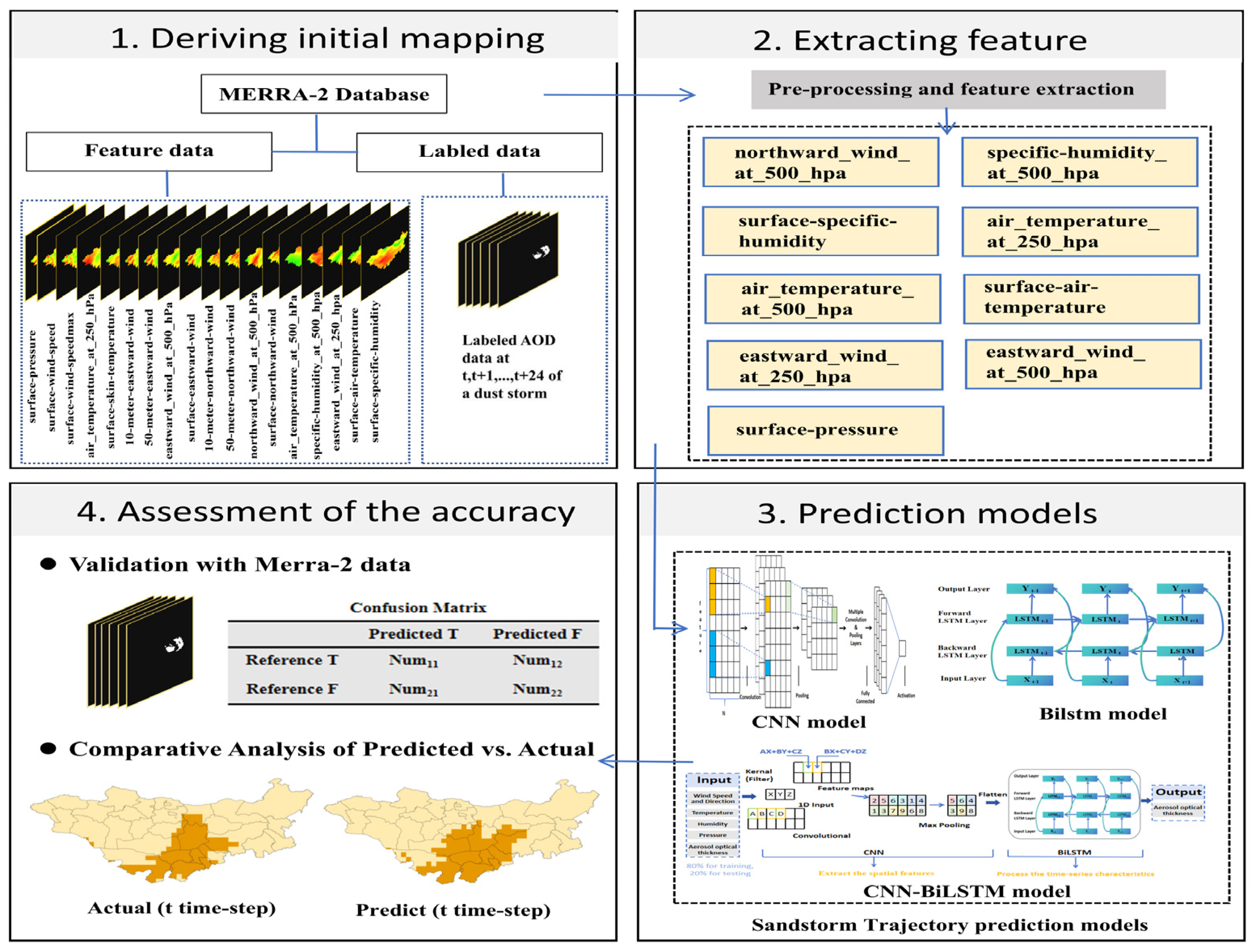
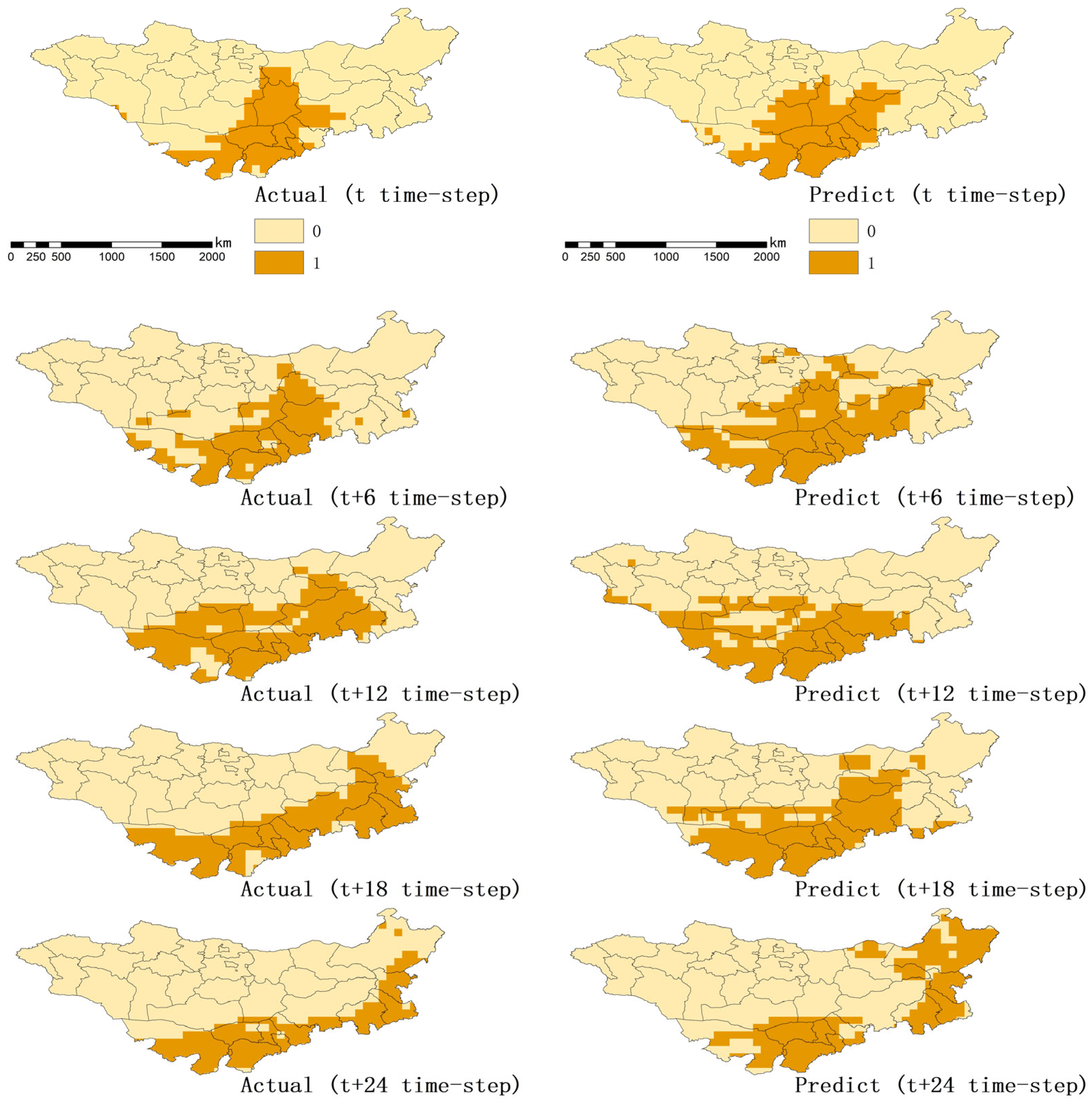
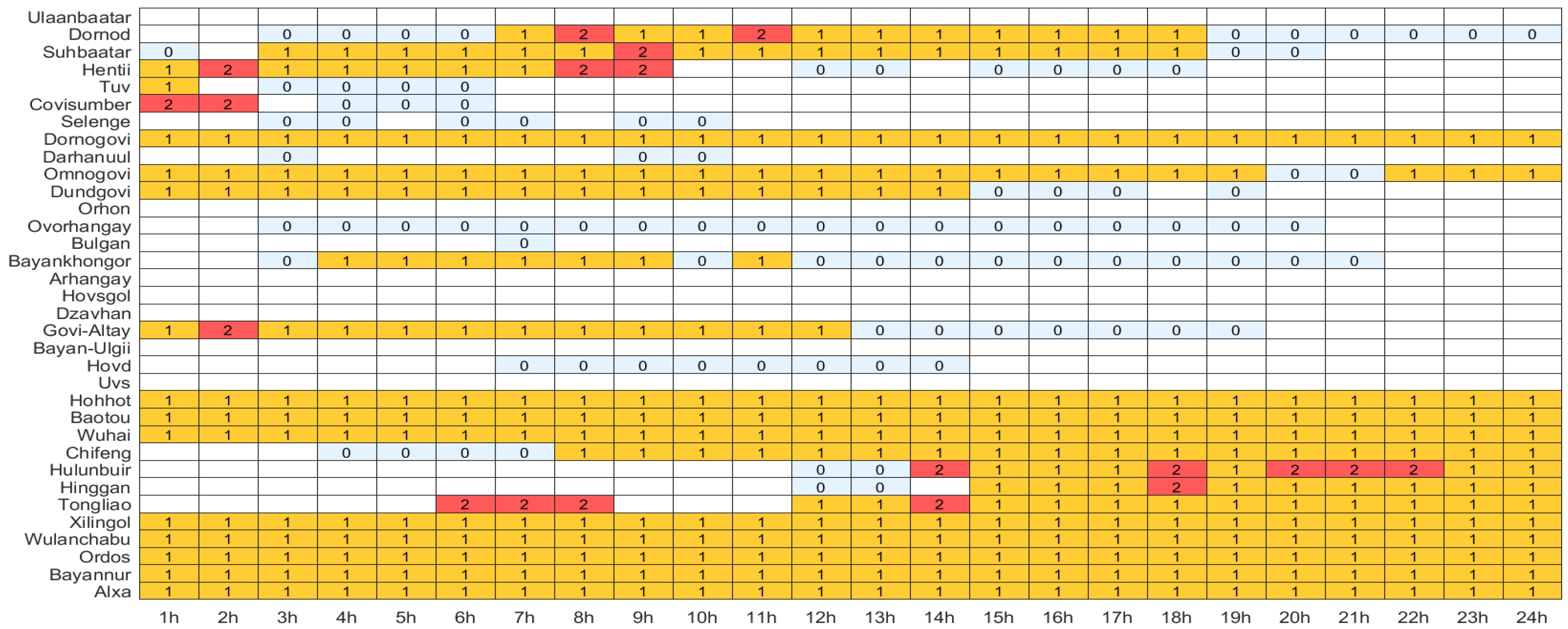
The sandstorm path prediction framework proposed in this study (Figure 2) consists of an input layer (multi-source data), feature optimization, a spatiotemporal modeling module (CNN–BiLSTM), and an output layer (24 h prediction image). During data preprocessing, the original dataset was divided into training, validation, and test sets. The model input consists of MERRA-2 AOD raw data at specific time steps combined with geographical environmental information, while the output corresponds to the predicted sandstorm distribution at the same time step. The labeled AOD layer was used as the prediction target during model training. The CNN layers are employed to efficiently extract local spatial features from multi-source remote sensing data, such as satellite imagery and atmospheric variables, which are crucial for capturing the dynamic pathways of dust storms. The BiLSTM layer robustly models both forward and backward dependencies in temporal sequences, making it well-suited to handle the spatiotemporal non-stationarity inherent in dust storm events. Compared to the Gated Recurrent Unit (GRU), which utilizes a simpler gating mechanism that may overlook subtle bidirectional dependencies in complex spatiotemporal data such as dust storm trajectories, our preliminary experiments indicate that BiLSTM improves prediction accuracy by approximately 2–4% on the validation set. In contrast to Transformer models, which excel at capturing global dependencies but often entail high computational costs and extended training times due to their self-attention mechanism, the hybrid CNN-BiLSTM approach achieves an optimal balance among spatial feature extraction, temporal dependency modeling, and computational efficiency. It is therefore better suited for real-time dust storm trajectory prediction based on remote sensing data in arid regions.

The CNN layers efficiently extract spatial features crucial for sandstorm path prediction, while the BiLSTM layers capture forward and backward dependencies in the time series, handling long time spans of data. Compared to GRU, BiLSTM provides a more comprehensive modeling of time dependencies, and, when compared to Transformer, CNN-BiLSTM outperforms in computational efficiency and training time. Moreover, by combining spatial feature extraction with temporal feature modeling, CNN-BiLSTM strikes a good balance, enhancing prediction accuracy while maintaining high computational efficiency.

The movement of sandstorms is strongly influenced by geographical background factors. Therefore, the AOD dataset and geographical background information were integrated to construct the input layer. Because this task involves a time-series problem, the input comprises hourly AOD images along with spatial background variables such as air pressure, temperature, wind speed, wind direction, and humidity, represented on a 71 × 81 pixel grid. The neural network was employed to extract spatiotemporal features from the input data, thereby generating sandstorm path predictions.

2.3.1. Overall Structure Design of the Model

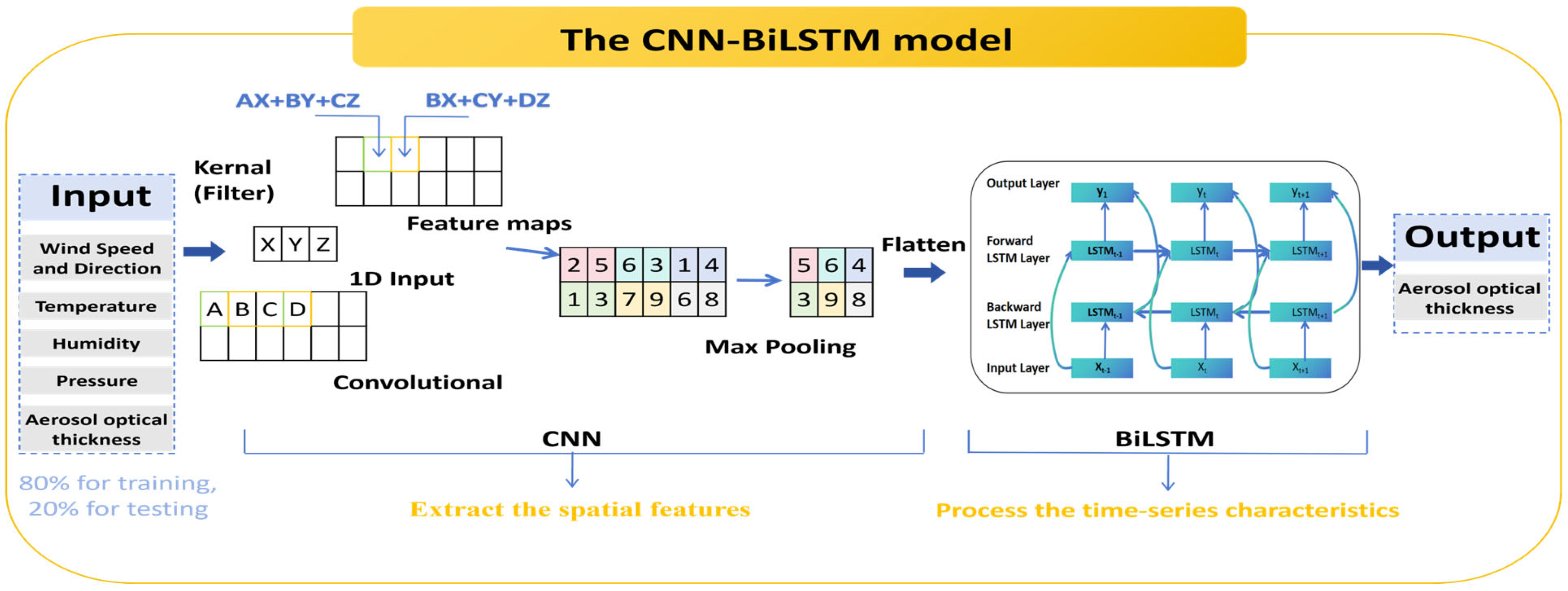
The CNN–BiLSTM is a deep learning architecture that integrates convolutional neural networks (CNNs) with bidirectional long short-term memory (BiLSTM) networks. In this architecture, spatial features are extracted through the CNN layers, temporal features are captured through the BiLSTM layers, and predictions are generated via fully connected and output layers. In a conventional 1D-CNN model, the fully connected layer cannot effectively utilize historical information and considers only the features of the current time step. In contrast, the BiLSTM model captures both forward and backward dependencies in sequence data, enabling a more comprehensive understanding of contextual relationships and thereby significantly improving model accuracy. The CNN layers efficiently extract spatial features crucial for sandstorm path prediction, while the BiLSTM layers capture forward and backward dependencies in the time series, handling long time spans of data. Compared to GRU, BiLSTM provides a more comprehensive modeling of time dependencies, and, when compared to Transformer, CNN-BiLSTM outperforms in computational efficiency and training time. Moreover, by combining spatial feature extraction with temporal feature modeling, CNN-BiLSTM strikes a good balance, enhancing prediction accuracy while maintaining high computational efficiency. The detailed structure of the CNN–BiLSTM model proposed in this study is illustrated in Figure 3.

The developed model comprises 16 layers, including five one-dimensional convolutional layers (Conv1D), two bidirectional LSTM (BiLSTM) layers, three max-pooling layers (MaxPooling1D), two fully connected (Dense) layers, two Dropout layers, and several normalization layers (LayerNormalization). These layers are organized into two primary modules: the feature extraction component and the prediction component. The feature extraction component consists of three convolutional blocks and two BiLSTM layers. In the first convolutional block, two Conv1D layers are applied, each containing 32 filters of size 5 × 1, with ReLU activation and L2 regularization to enhance model generalization. Dimensionality reduction is achieved using MaxPooling1D, while a Dropout layer is applied to prevent overfitting. The second convolutional block includes two Conv1D layers, each with 64 filters of size 3 × 1, employing the same activation, L2 regularization, pooling, and Dropout strategies. The third convolutional block contains one Conv1D layer with 128 filters of size 3 × 1, followed by activation, L2 regularization, pooling, and Dropout. HeUniform initialization was adopted for convolutional layers to enhance stability and convergence efficiency during training. Two BiLSTM layers, each with 128 neurons, simultaneously capture forward and backward dependencies in the sequence, thereby strengthening the model’s ability to learn time-dependent features. L2 regularization was also applied to the BiLSTM layers to reduce the risk of overfitting.

The prediction module comprises two fully connected layers, each with 128 neurons and ReLU activation for nonlinear transformation. A Dropout layer was inserted between the two fully connected layers to prevent overfitting. The output layer employs a softmax activation function, which interprets the outputs as a probability distribution across categories, thereby providing the predicted probability for each class. The model contained a total of 757,346 trainable parameters during training.

2.3.2. Spatial Feature Extraction Module (CNN)

Inspired by biological visual perception (Fukushima, 1980) [29], convolutional neural networks (CNNs) were first proposed by LeCun et al. [30] in 1989 and demonstrated significant performance improvements over traditional fully connected neural networks [31]. CNNs are widely applied in two-dimensional data processing, such as image and video analysis, by incorporating local receptive fields, weight sharing, and pooling mechanisms to reduce parameters and improve computational efficiency.

In recent years, CNNs have been extended to one-dimensional CNNs (1D CNNs) to meet the modeling requirements of sequence data, such as speech, vibration, and environmental time-series data [32]. One-dimensional CNNs retain key structures, such as convolution and pooling, while exhibiting low computational complexity and strong local feature extraction capability, making them particularly suitable for processing time-series signals. The basic structure is illustrated in Figure 4. It primarily consists of multiple convolution and pooling layers, followed by fully connected and output layers. Network parameters are typically optimized using backpropagation and stochastic gradient descent (SGD) methods [33].

2.3.3. Time Feature Modeling Module (BiLSTM)

The bidirectional long short-term memory (BiLSTM) network is a variant of the LSTM. By introducing forward and backward propagation paths and capturing contextual information in both directions, it effectively addresses long-term dependency problems while reducing the risk of gradient vanishing, thereby enhancing its ability to model temporal features [34]. The LSTM addresses the short-term memory limitations of recurrent neural networks (RNNs) through a gating mechanism that regulates information flow. The internal structure of the LSTM is illustrated in Figure 5a, where the cell state at each time step is updated and propagated through gating mechanisms. The structure of the BiLSTM is presented in Figure 5b, comprising a forward LSTM layer and a backward LSTM layer to fully exploit interdependencies within the time series.

In contrast, CNNs exhibit limitations when processing one-dimensional data, including handling variable time-series lengths, susceptibility to local perception problems, and difficulty in effectively modeling temporal correlations. BiLSTMs, however, offer advantages such as capturing long-term dependencies, robust modeling capabilities, and flexible handling of time-series data. These characteristics enable BiLSTMs to compensate for the limitations of CNNs in processing and predicting one-dimensional time-series data.

2.3.4. Model Training and Optimization Strategy

Machine learning models typically involve numerous hyperparameters. Accurate prediction with the CNN–BiLSTM model requires careful adjustment of multiple hyperparameters, which significantly influence network performance [35]. In this study, a batch size of 16 was determined through hyperparameter tuning. The Adam optimizer was employed during training, with the learning rate set to 2 × 10⁻⁴. 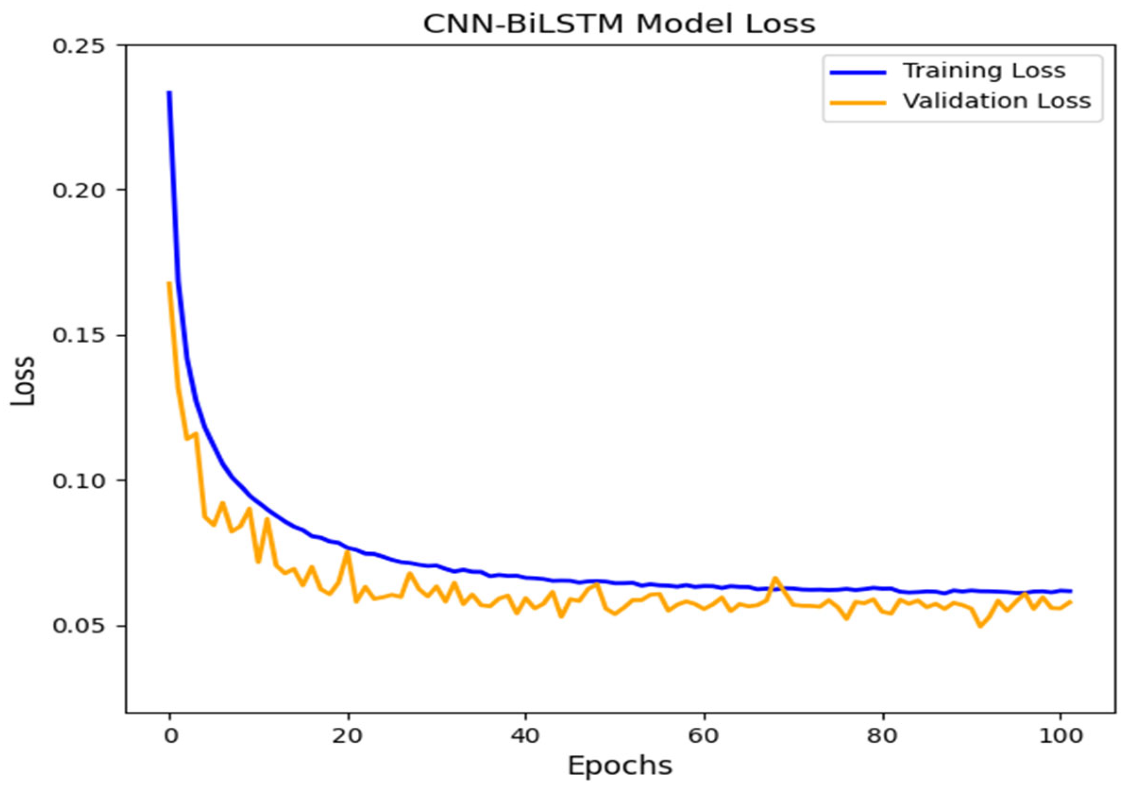To improve the model’s ability to distinguish rare and unpredictable samples in sandstorm path prediction, while suppressing the dominance of easily classified samples during training, Focal Loss was introduced as the optimization objective, based on the standard cross-entropy (CE) loss function [36]. To verify generalization ability and prevent overfitting, the dataset was divided into training, validation, and test sets in a 70%:20%:10% ratio. During training, an early stopping strategy (patience = 60, min_delta = 1 × 10⁻⁴) was implemented to terminate training when validation performance ceased to improve.

During training, the minimum validation loss was recorded as the optimal weight, and the model parameters corresponding to the best performance were retained after completion. The evaluation system incorporated multiple performance metrics, including overall accuracy, F1-score, precision, recall, and ROC-AUC, providing a reliable quantitative basis for model assessment.

2.4. Evaluation Methods

The objective of this study is to accurately predict the movement path of sandstorms, despite the substantial imbalance between positive and negative samples. Therefore, overall accuracy, F1-score, precision, recall, and AUC were selected as evaluation metrics to quantitatively assess the performance of the CNN–BiLSTM model. Given that sandstorms are hazardous weather events, higher recall is prioritized over precision in order to reduce missed detections. Overall accuracy reflects the general classification performance of the model. The F1-score is particularly important for balancing precision and recall, while AUC provides an effective measure of the model’s ability to distinguish between positive and negative classes.

Overall accuracy and the F1-score were derived from the confusion matrix. Overall accuracy represents the proportion of correctly classified pixels, defined as the ratio of correctly classified pixels to the total number of pixels. The calculation method for this metric is presented in Formula (2).

$$OverallAccuracy=\left({\displaystyle \frac{TP+TN}{TP+FP+FN+TN}}\right)\times 100\%,$$

(2)

True Positive (TP) denotes instances correctly predicted as positive, whereas True Negative (TN) denotes instances correctly predicted as negative. Conversely, False Positive (FP) represents cases in which negative samples are incorrectly predicted as positive (Type I error), while False Negative (FN) represents cases in which positive samples are incorrectly predicted as negative (Type II error). The F1-score is a metric used to balance precision and recall, and is calculated using Formula (3).

$$F1\left(\%\right)=\left({\displaystyle \frac{2\times Precision\times Recall}{Precision+Recall}}\right)\times 100\%,$$

(3)

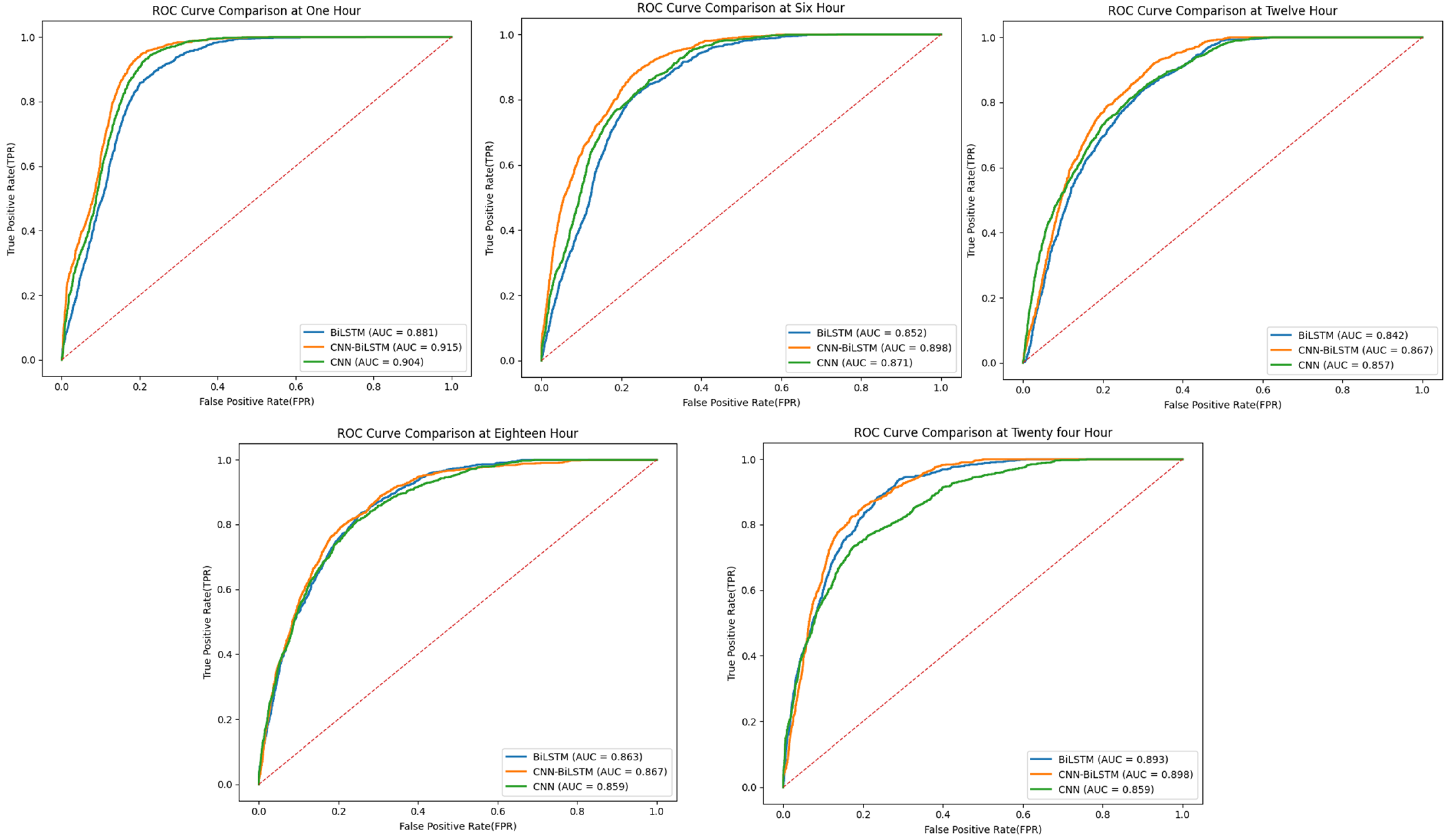
The area under the receiver operating characteristic curve (AUC) is an important indicator of a model’s classification ability. It quantifies the ability of the model to distinguish between classes. AUC values range from 0 to 1, with values closer to 1 indicating stronger discriminative power. In this study, AUC corresponds to the area under the ROC curve, with larger values indicating better classification performance. AUC was used to evaluate the model’s effectiveness in classifying sandstorm occurrence points (positive class) and non-occurrence points (negative class).

Accuracy and recall were calculated using Formula (4) and Formula (5), respectively:

$$Precision\left(\%\right)=\left({\displaystyle \frac{TP}{TP+FP}}\right)\times 100\%,$$

(4)

$$Recall\left(\%\right)=\left({\displaystyle \frac{TP}{TP+FN}}\right)\times 100\%$$

(5)

3. Results

3.1. Analysis of Model Performance and Learning Curve

Figure 6 illustrates the changes in the loss function for training and validation data over 100 epochs. The learning curve trend can be used to diagnose the effect of training on model performance. As shown in Figure 6, the overall loss function exhibits a downward trend, indicating good model performance. During the initial epoch, both training and validation loss under Focal Loss decreased sharply. As training progressed, the rate of decrease gradually slowed and eventually converged. Typically, a gap exists between the learning curves of training and validation loss. In an ideal fit, the validation loss decreases to a stable point with only a small gap relative to the training loss [37].

3.2. Feature Selection Analysis Based on RFFI

Random Forest Feature Importance (RFFI) was applied to select and optimize geographical background information. This information plays a critical role in the occurrence and movement of sandstorms and is essential for improving prediction accuracy. Figure 7 presents the RFFI results, with feature stability represented by error bars. According to the feature importance scores, upper-air humidity at 500 hPa exerts the greatest influence, followed by the southerly wind component (V-component) at 500 hPa, indicating that both variables play critical roles in the occurrence and movement of sandstorms. In addition, air temperature, the easterly wind component (U-component), and pressure at 250 hPa and 500 hPa also exhibit high importance. Surface specific humidity and surface skin temperature likewise show strong influence, indicating that surface characteristics cannot be neglected in sandstorm formation. The importance of the southerly wind is more pronounced than that of the northerly wind, particularly at 500 hPa. The southerly wind exerts a stronger influence on sandstorm trajectories, potentially facilitating their northward spread. Smaller error bars indicate stable feature influence in the model, whereas larger error bars suggest greater variability in predictive contribution. The first nine features exhibit shorter error bars, indicating a stable impact on model performance. In contrast, features such as ULML, SPEEDMAX, and U50M display larger error bars, reflecting instability in model prediction. The high importance of humidity variables reflects the critical role of moisture in the hygroscopic growth and sedimentation of dust particles. Regarding the influence of atmospheric circulation, dust events are often associated with specific synoptic patterns, such as the development of Mongolian cyclones, the movement of the Siberian High, and variations in the intensity of the mid-latitude westerly jet.

Therefore, in this study, key variables such as upper-air temperature, southerly wind, surface pressure, easterly wind, and humidity were primarily considered, while less contributive factors such as surface wind speed and low-level wind direction were excluded. Insignificant and unstable variables were eliminated to optimize model performance and improve prediction accuracy. It should be noted that, in this analysis, the U and V wind components represent easterly and southerly wind vectors, respectively.

3.3. Model Evaluation and Multi-Time Scale Prediction Performance Analysis

In this study, a CNN-BiLSTM model was constructed to predict sandstorms, with the objective of evaluating classification performance across different prediction time horizons. Figure 8 presents the confusion matrices generated by the model at prediction times of t, t+6 h, t+12 h, t+18 h, and t+24 h. These results are based on geographical and environmental features, including upper-air temperature, 500 m wind direction, surface skin temperature, and relative pressure, thereby illustrating the model’s classification performance under varying forecast lead times.

As shown in Figure 8, the classification accuracy of the model for the dust category consistently remained above 80%, with specific values of 84.17%, 79.54%, 82.02%, 83.33%, and 87.13%. The maximum fluctuation range was only 7.74%, demonstrating strong stability in the identification of positive samples. In contrast, the classification accuracy for the non-dust category exhibited a downward trend, declining from 87.67% at time t to 73.73% at t+12 h, and reaching the lowest value of 73.01% at t+18 h, before slightly rebounding to 75.78% at t+24 h. Overall, the accuracy decreased by 14.66 percentage points from t to t+18 h. These results suggest that with increasing prediction lead time, the model’s ability to discriminate non-dust events is notably reduced, which may be attributed to the pronounced spatial heterogeneity of dust events in the study region and the significant imbalance between dust and non-dust pixel proportions.

To further validate the effectiveness of the proposed architecture, the performance of CNN-BiLSTM was compared with that of CNN and BiLSTM at different time horizons. As shown in

Table 2. The results of CNN, BiLSTM, and CNN-BiLSTM models in the sandstorm movement path prediction task.

T	Indices	CNN	BiLSTM	CNN-BiLSTM
One hour	Overal accuracy	0.8163	0.8166	0.8461
	F1 Score	0.8428	0.8413	0.8656
	AUC	0.9035	0.8808	0.9155
Six hour	Overal accuracy	0.7720	0.7752	0.8011
	F1 Score	0.8060	0.8081	0.8289
	AUC	0.8808	0.8518	0.8977
Twelve hour	Overal accuracy	0.7449	0.7625	0.8079
	F1 Score	0.7792	0.7921	0.8277
	AUC	0.8573	0.8415	0.8666
Eighteen hour	Overal accuracy	0.8021	0.8068	0.8205
	F1 Score	0.8284	0.8317	0.8423
	AUC	0.8586	0.8630	0.8674
Twenty-four hour	Overal accuracy	0.8317	0.8334	0.8607
	F1 Score	0.8541	0.8572	0.8776
	AUC	0.8588	0.8927	0.8982

and Figure 9, CNN-BiLSTM consistently outperformed the other two models across all three metrics—accuracy, F1-score, and AUC. Notably, at the 24 h horizon, CNN-BiLSTM achieved an accuracy of 0.8588, an F1-score of 0.8927, and an AUC of 0.8982, which are 3.9%, 1.5%, and 1.4% higher than CNN, and 2.1%, 1.5%, and 1.4% higher than BiLSTM, respectively. The optimal performance observed at this horizon may be related to a more class-distinctive distribution of features at the 24 h time point, which facilitates more effective feature recognition by the model. Moreover, CNN-BiLSTM achieved consistently higher AUC values across all time windows, confirming that the integration of CNN and BiLSTM enables robust classification sensitivity even under the highly imbalanced distribution of positive and negative samples.

In the test set (9 April 2024), Figure 10 presents a comparison between the predicted and actual sandstorm distributions at hours 1, 6, 12, 18, and 24.

3.4. Accuracy Analysis and Hourly Statistics of Urban Sandstorm

In order to further reveal the movement path and spatiotemporal heterogeneity of sandstorm events over the Mongolian Plateau, a comparative analysis was conducted on the impact of sandstorms on major cities at different times using observed data and model predictions from 9 April 2023, in the test set. Figure 11 illustrates the distribution of sandstorm impacts on cities between 01:00 and 24:00 as a heat map. The vertical axis represents the major cities in the study area, the horizontal axis denotes the hourly time series, and the cell values indicate the occurrence of sandstorms at each time point (0 represents a false negative, 1 a correct prediction, and 2 a false positive).

The model successfully reproduced the temporal occurrence and spatial distribution of sandstorms in Alxa League, Ulanqab, Ordos, and other locations within the primary affected regions on 9 April 2023. The simulation of time-series variations along the propagation paths in South Gobi and East Gobi was also relatively accurate. In the central region of Mongolia, such as Tubu, Central Province, and Ulaanbaatar, predictions were made in advance, demonstrating an “early warning” capability; in contrast, in northeastern regions such as Hulun Buir and Xing’an League, delays and misclassifications were observed, suggesting that the temporal response capability at the margins requires further improvement. In summary, the model demonstrated strong predictive accuracy in the southern part of the Mongolian Plateau and in the western and central regions of Inner Mongolia, and it effectively captured the core movement path and temporal structure of the sandstorm event on that day.

4. Discussion

The results of this study indicate that the time dimension cannot be overlooked in the construction of dust weather prediction models. Although both CNN-BiLSTM and CNN models account for spatial features, the predictive performance of the CNN-BiLSTM model surpasses that of the CNN model. Further analysis of model performance across different time scales revealed that the CNN-BiLSTM model showed the greatest improvement in predictive accuracy at the 12 h forecast horizon, where overall accuracy increased by 6.3% and the F1 score by 4.85%. This may be because the BiLSTM structure can effectively capture contextual information in long time series and exhibits stronger memory capacity for processes above the mesoscale. As this study did not account for the dynamic changes of ground dust sources, the model was entirely dependent on MERRA-2 background meteorological variables, potentially affecting model stability under abnormal or missing input conditions. In the future, initial conditions could be optimized by incorporating the remote sensing dust source index.

The CNN-BiLSTM model demonstrates advantages over numerical models in feature learning and in capturing nonlinear relationships from large datasets, which is consistent with the findings of Ren et al. [38]. In numerical model forecasts of dust weather, the parameterization scheme of sand emission remains a critical and challenging component directly linked to forecasting performance. Deep learning methods circumvent this issue and can leverage their strengths to correct deviations in numerical model outputs, particularly nonlinear deviations. Thus, it is feasible to utilize deep learning approaches to construct predictive models. For instance, in the case of the HYSPLIT model, predictive performance is highly dependent on the accuracy of meteorological inputs and is highly sensitive to variations in initial conditions. Moreover, the model is relatively simplistic in trajectory tracking, making it inadequate for handling complex and variable sandstorm dynamics, particularly in short-term forecast scenarios with high spatial and temporal resolution. Compared with the AUC of 0.78 obtained by Kim et al. based on the HYSPLIT model, the model proposed in this study achieved an AUC of 0.91 under similar conditions, demonstrating superior discriminative ability [39]. Current research on the movement pathways of dust storms over the Mongolian Plateau has primarily focused on their sources, propagation characteristics, and spatial extent, yet there remains a lack of consistent quantitative assessment regarding prediction accuracy [5,9]. Several studies have employed the HYSPLIT model to analyze Himawari-8 satellite imagery from 2016 to 2020, enabling the statistical characterization of dust storm events (DSEs) in terms of source regions, affected areas, and transport trajectories, followed by simulation and validation. It has been widely reported that the HYSPLIT model demonstrates relatively high accuracy in simulating dust storm propagation paths, particularly at meteorological stations located along major transport routes, where it provides reliable simulations of dust event movement and regional impact assessments [40].

As dust weather events are highly complex, numerous related factors exhibit distinct variations before, during, and after such events. Regional differences in the causes of dust weather further influence prediction accuracy. In future research, the proposed model could be integrated into regional environmental management platforms through the combination of real-time remote sensing monitoring and short-term numerical forecasting models, enabling rolling prediction and dynamic early warning of sandstorm paths in key urban agglomerations.

Moreover, the model still has room for improvement in spatio-temporal feature extraction. Although CNN can effectively capture local spatial features, its inductive bias is mainly limited to translation invariance, and the receptive field of the convolution kernel is limited. In future work, Graph Convolutional Networks (GCNs) can be considered to enhance the ability of spatial feature extraction. There is a significant spatial coupling relationship between the meteorological conditions in the moving surrounding area of the dust storm, and the traditional convolution operation is difficult to fully capture such complex spatial interactions. By constructing an adjacency matrix to aggregate neighborhood information, a GCN generates more representative node feature vectors, which can extract spatial structure features more effectively. Its nonlinear relationship modeling ability based on non-Euclidean space is expected to further improve the accuracy of dust storm path prediction. Therefore, the development of a hybrid model combining CNN and GCN will be an important research direction to improve the spatio-temporal prediction ability of dust storms.

5. Conclusions

This study proposes a deep learning framework that integrates CNN and BiLSTM, which can effectively predict the movement paths of sandstorms in the Mongolian Plateau over the next 1–24 h. The model uses AOD, wind direction, temperature, and humidity from MERRA-2 data as input variables and considers both geographical background and temporal information. The mean AUC exceeds 0.89 across multiple time scales, while the F1 score remains consistently above 0.83, effectively capturing the spatiotemporal distribution characteristics of dust events and demonstrating strong generalization ability and practical application potential.

Compared to existing datasets, the MERRA-2 reanalysis features hourly temporal resolution and global coverage, enabling hourly prediction of dust storm transport pathways. The proposed model consistently maintains high predictive accuracy across various time steps, demonstrating strong adaptability. This study provides valuable data support and a methodological reference for early warning and disaster prevention of dust storms in the Mongolian Plateau and surrounding regions.