Efficient Conditional Diffusion Model for SAR Despeckling

Abstract

Speckle noise inherent in Synthetic Aperture Radar (SAR) images severely degrades image quality and hinders downstream tasks such as interpretation and target recognition. Existing despeckling methods, both traditional and deep learning-based, often struggle to balance effective speckle suppression with structural detail preservation. Although Denoising Diffusion Probabilistic Models (DDPMs) have shown remarkable potential for SAR despeckling, their computational overhead from iterative sampling severely limits practical applicability. To mitigate these challenges, this paper proposes the Efficient Conditional Diffusion Model (ECDM) for SAR despeckling. We integrate the cosine noise schedule with a joint variance prediction mechanism, accelerating the inference speed by an order of magnitude while maintaining high denoising quality. Furthermore, we integrate wavelet transforms into the encoder’s downsampling path, enabling adaptive feature fusion across frequency bands to enhance structural fidelity. Experimental results demonstrate that, compared to a baseline diffusion model, our proposed method achieves an approximately 20-fold acceleration in inference and obtains significant improvements in key objective metrics. This work contributes to real-time processing of diffusion models for SAR image enhancement, supporting practical deployment by mitigating prolonged inference in traditional diffusion models through efficient stochastic sampling.

1. Introduction

Synthetic Aperture Radar (SAR) acquires electromagnetic scattering information from the Earth’s surface by transmitting and receiving microwave signals. Operating independently of illumination and meteorological conditions, it has become an indispensable technology for critical remote sensing applications, including disaster monitoring, vegetation structure inversion, and urban deformation detection [1]. However, the coherent nature of SAR imaging generates speckle noise through random interference of signals within each resolution cell. Speckle not only degrades the signal-to-noise ratio (SNR) of the imagery but also disrupts the local statistical homogeneity of scene features, obscuring structural edges and fine-grained textures [2]. By distorting class boundaries and masking target signatures, speckle systematically impairs the accuracy and reliability of critical downstream tasks such as land-cover classification, target detection [3], and change detection [4]. Therefore, developing advanced algorithms that achieve effective speckle suppression while maximally preserving structural and radiometric fidelity is paramount for enhancing the performance and robustness of high-level SAR applications.

Historically, research in SAR despeckling has progressed along three primary paradigms: local statistical filtering, transform-domain filtering, and non-local filtering. Local statistical filters operate by performing adaptive pixel-wise smoothing within a localized window [5]. This class of algorithms is exemplified by seminal works such as the Lee [6], Frost [7], Kuan [8], and Gamma-MAP [9] filters. While computationally efficient, their inherent locality imposes a fundamental trade-off: in homogeneous regions, they tend to blur subtle textures, whereas in heterogeneous areas, they often fail to preserve sharp edges and strong scatterers. The transform-domain paradigm for despeckling often begins within a homomorphic framework, where a logarithmic transform is first applied to linearize the multiplicative speckle into an additive noise model [10]. Subsequently, multi-scale geometric transforms [11] are employed to decompose the image, allowing for coefficient shrinkage to suppress noise while preserving structural information. To address the non-adaptive nature of conventional hard/soft thresholding, subsequent research pivoted towards more sophisticated statistical modelling. These strategies ranged from deriving adaptive shrinkage operators based on probability mixture models [12] to imposing spatial contextual constraints on wavelet coefficients via Markov Random Fields [13] and even transplanting classical Wiener filtering theory into the stationary wavelet domain to seek an optimal estimate [14]. However, a critical limitation of these “model-driven” methods is their reliance on fixed statistical priors, which are often inadequate for capturing the full spectrum of complex heterogeneity in real SAR scenes [15]. Non-local methods exploit Non-Local Self-Similarity by globally identifying similar patches for weighted filtering. The Non-Local Means algorithm [16] pioneered this approach, denoising via weighted averaging of similar patches to preserve fine details. For multiplicative speckle in SAR images, the Probabilistic Patch-Based (PPB) method [17] incorporated Gamma-distributed likelihood, aligning patch similarity with the noise model. This evolved into SAR-BM3D [18], which integrated a SAR-optimized similarity metric into the Block-Matching and 3D (BM3D) collaborative filtering framework, effectively balancing texture preservation and speckle suppression. However, this series of methods is typically limited by filtering parameter design and similarity criteria, incurring high computational costs [19]. These inherent bottlenecks have driven the shift toward data-driven deep learning paradigms.

In recent years, deep learning has become the benchmark for numerous image processing tasks [20]. SAR-CNN [21], proposed by Chierchia et al., pioneers the application of Convolutional Neural Networks (CNNs) to SAR image despeckling, employing a 17-layer residual network to generate despeckled images. Subsequently, ID-CNN [22] leverages synthetic speckle in optical images for supervision, optimizing a combined Euclidean loss and Total Variation (TV) regularizer to achieve smoother restoration without logarithmic transformation. SAR-DRN [23] integrates dilated convolutions into residual blocks with skip connections to address vanishing gradients, enhancing robustness in high-noise scenarios. MONet [24] employs a composite loss function integrating pixel-wise Mean Squared Error (MSE), Kullback–Leibler (KL) divergence, and a term preserving strong scatterers, enabling synergistic optimization of texture preservation and speckle statistical consistency across homogeneous, heterogeneous, and extremely heterogeneous regions. Introduced in 2017 [25], the Transformer framework established an effective approach for capturing long-range dependencies. Trans-SAR [26] pioneered the use of the hierarchical Vision Transformer for SAR despeckling, outperforming contemporary CNN-based models. Subsequently, SAR-CAM [27] introduced a Continuous Attention Module (CAM) and a Contextual Block (CB), significantly enhancing the representation of critical features.

Due to the absence of genuine speckle-free SAR images, early methods primarily generated synthetic samples by overlaying Gamma noise on optical images for supervised training. Subsequently, SAR2SAR [28] exploited noise redundancy to develop an unsupervised framework, eliminating the need for clean ground truth. Speckle2Void [29] utilized blind-spot CNNs and Bayesian posterior reconstruction for single-image self-supervision. Beyond unsupervised approaches, researchers have investigated high-SNR “pseudo ground truth” from multi-temporal images of the same scene to enable supervised training. For example, Vitale et al. [30] proposed a two-stage training strategy: pre-training on synthetic data followed by domain-adaptive fine-tuning via multi-temporal interferometric phase fusion.

In recent years, the proliferation of generative models in image processing has highlighted the potential of Generative Adversarial Networks (GANs) for SAR despeckling, optimizing perceptual quality and distributional consistency via adversarial learning between generator and discriminator [31]. More recently, Denoising Diffusion Probabilistic Models (DDPMs), prized for stable training and superior detail synthesis, have been applied to SAR despeckling. SAR-DDPM [32] pioneered DDPM adoption for this task. Building thereon, Diffusion SAR developed a conditional DDPM in the log-Yeo-Johnson transform domain [33]. Concurrently, Pan et al. [34] incorporated Swin Transformer Blocks into the noise predictor and introduced Pixel-Shuffle Down-sampling (PD) Refinement to address the domain gap.

However, existing methods—whether CNN- or Transformer-based—still struggle to balance noise suppression with information fidelity (i.e., preserving textures and structures). Although diffusion models have achieved breakthroughs in quantitative metrics, they introduce new challenges: artifacts and blurring persist in fine detail reconstruction, and the enormous inference overhead from thousands of iterative sampling steps poses a major barrier to practical application. Thus, developing a SAR despeckling model that simultaneously ensures high image fidelity (in terms of textures and structures) and high inference efficiency remains a core challenge urgently requiring resolution in this field.

To address the aforementioned challenges, this paper proposes the Efficient Conditional Diffusion Model, a framework that systematically enhances the comprehensive performance of SAR image despeckling through three key contributions:

An Efficient Inference Framework: We design a denoising network that jointly predicts noise components and variance parameters, enabling accelerated sampling through optimized timestep scheduling. This approach achieves 20× speedup in inference time while maintaining denoising quality. A Highly Effective Network Architecture: We integrate discrete wavelet transforms into the encoder’s downsampling stages, providing lossless frequency decomposition and multi-scale feature representation. This design preserves structural information more effectively during the despeckling process. An Efficacious Training Strategy: We employ pre-training on synthetic data followed by fine-tuning on real multi-temporal SAR images, effectively bridging the domain gap between synthetic training data and real-world SAR scenarios.

The remainder of this paper is organized as follows. Section 2 reviews the mathematical modeling of SAR speckle noise and the foundational principles of Denoising Diffusion Probabilistic Models (DDPMs). Section 3 details our proposed method, including its network architecture, efficient inference strategy, and loss function design. Section 4 presents comprehensive experimental results, encompassing quantitative comparisons and qualitative assessments on both synthetic and real-world SAR datasets. Section 5 conducts a series of ablation studies to systematically validate the effectiveness of key components in our model and the accelerated sampling strategy. Finally, Section 6 concludes the paper and outlines potential future research directions.

2. Related Works

2.1. SAR Speckle Model

While enabling high-resolution imaging through coherent processing, Synthetic Aperture Radar (SAR) inherently produces speckle noise. This noise arises from the coherent superposition of echoes from multiple elementary scatterers within a resolution cell, resulting in random interference due to their varying phases. Consequently, speckle noise exhibits multiplicative characteristics, being coupled with signal intensity, and is spatially correlated. It is mathematically modeled as [35]:

$$X=Y\cdot N$$

(1)

where $X$ denotes the SAR image corrupted by speckle noise; $Y$ represents the ideal noise-free reflectivity; and $N$ signifies the speckle noise generated during the SAR imaging process. The speckle noise $N$ typically follows a Gamma distribution, with its probability density function (PDF) expressed as:

$$P\left(N\right)={\displaystyle \frac{L^L{N}^{L-1}{e}^{-LN}}{\Gamma \left(L\right)}}$$

(2)

where $L$ represents the Equivalent Number of Looks (ENL), $\Gamma \left(L\right)$ denotes the Gamma function, and the noise $N$ is characterized by a mean of 1 and a variance of $1/L$. Given the complex statistical properties of multiplicative speckle in SAR imagery, a comprehensive evaluation of denoising algorithm performance must consider four key dimensions: speckle suppression, structural fidelity, radiometric fidelity, and artifact suppression [36].

2.2. Diffusion Models for SAR Despeckling

Denoising Diffusion Probabilistic Models (DDPMs) are a class of deep generative models inspired by non-equilibrium thermodynamics [37]. They define a forward diffusion process and a learnable reverse denoising process, both modeled as Markov chains, as shown in Figure 1.

The forward diffusion process gradually adds noise to the input data. It is modeled as a predefined Markov chain, starting from an input image $x_0$ and iteratively injecting Gaussian noise at each step until the signal is fully obscured. The forward transition distribution for a single step is defined as:

$$q\left(x_t|x_{t-1}\right)=\mathcal{N}\left(x_t;\sqrt{1-{\beta }_t}{x}_{t-1},{\beta }_{t}I\right)$$

(3)

where ${\beta }_t\in \left(0,1\right)$ is a pre-defined variance schedule that governs the noise level at each timestep $t$. This transition kernel indicates that the state $x_t$ is obtained by scaling the preceding state $x_{t-1}$ by $\sqrt{1-{\beta }_t}$ and adding Gaussian noise with variance ${\beta }_t$. Through the reparameterization trick, a noisy version of the initial state $x_0$ at an arbitrary timestep t can be directly sampled:

$$q\left(x_t|x_0\right)=\mathcal{N}\left(x_t;\sqrt{{\overline{\alpha }}_t}{x}_0,\left(1-{\overline{\alpha }}_t\right)I\right)$$

(4)

where ${\alpha }_t=1-{\beta }_t$, ${\overline{\alpha }}_t={{\displaystyle \prod }}_{s=1}^t{\alpha }_s$. For a sufficiently large $T$ and a well-designed schedule, $x_T$ converges to a standard isotropic Gaussian distribution $\mathcal{N}\left(0,I\right)$. This property yields a closed-form expression for generating training samples, which forms the cornerstone of the entire training procedure:

$$x_t=\sqrt{{\overline{\alpha }}_t}{x}_0+\sqrt{1-{\overline{\alpha }}_t}ϵ$$

(5)

In the task of Synthetic Aperture Radar (SAR) image despeckling, our objective is to learn a mapping from a noisy observation $y$ to its corresponding noise-free ground truth $x_0$. The Conditional Denoising Diffusion Probabilistic Model (Conditional DDPM) offers a powerful generative framework for this purpose. Its core idea is that, since the true reverse process $q\left(x_{t-1}|x_t,y\right)$ is intractable due to its dependence on the entire data distribution, the model approximates it via a learned parameterized reverse Markov chain. This chain starts from standard Gaussian noise $x_T\sim \mathcal{N}\left(0,I\right)$ and, guided explicitly by the condition $y$, progressively recovers $x_0$. Each step in this reverse process is modeled as a conditional Gaussian distribution parameterized by a neural network:

$$p_{\theta }\left(x_{t-1}|x_t,y\right)=\mathcal{N}\left(x_{t-1};{\mu }_{\theta }\left(x_t,y,t\right),{\Sigma }_{\theta }\left(x_t,y,t\right)\right)$$

(6)

Theoretically, the true posterior $q\left(x_{t-1}|x_t,x_0\right)$ is also Gaussian, providing justification for our parameterized form. Ho et al. [37] showed that, with a specific parameterization, the mean ${\mu }_{\theta }$ can be derived from a neural network ${ϵ}_{\theta }$ trained to predict the noise $ϵ$:

$${\mu }_{\theta }\left(x_t,y,t\right)={\displaystyle \frac{1}{\sqrt{{\alpha }_t}}}\left(x_t-{\displaystyle \frac{{\beta }_t}{\sqrt{1-{\overline{\alpha }}_t}}}{ϵ}_{\theta }\left(x_t,y,t\right)\right)$$

(7)

For the predictive variance ${\Sigma }_{\theta }$, the original work set it as a fixed hyperparameter, such as ${\Sigma }_{\theta }={\tilde{\beta }}_{t}I$ or ${\Sigma }_{\theta }={\beta }_{t}I$. In SAR despeckling, subsequent studies like Perera et al. [32] and Pan et al. [34] also adopted this fixed-variance approach.

The model’s training objective is derived by optimizing the variational lower bound (VLB). As demonstrated by Ho et al. [37], this objective can be simplified to an equivalent, more intuitive loss function, whose core principle is to train a network for predicting the added noise at each timestep. For our conditional task, this loss function is formulated as:

$${\mathcal{L}}_{simple}={\mathbb{E}}_{t,x_0,y,ϵ}\left[\parallel ϵ-{ϵ}_{\theta }\left(\sqrt{{\overline{\alpha }}_t}{x}_0+\sqrt{1-{\overline{\alpha }}_t}ϵ,y,t\right){\parallel }^2\right]$$

(8)

2.3. Comparison of Linear and Cosine Noise Schedules

The noise schedule ${\beta }_t$ is a critical design choice that governs model performance and training dynamics. It precisely dictates the signal decay trajectory during the forward process, thereby profoundly impacting the quality of the diffusion process and the stability of training [38]. The linear and cosine schedules are two predominant strategies, which, as depicted in Figure 2, exhibit marked differences in their control of the Signal-to-Noise Ratio (SNR). The linear schedule, originally proposed by Ho et al. [37], is defined as:

$${\beta }_t={\beta }_{\min }+{\displaystyle \frac{t-1}{T-1}}\left({\beta }_{\max }-{\beta }_{\min }\right)$$

(9)

where ${\beta }_{\min }$ and ${\beta }_{\max }$ are the minimum and maximum noise levels, respectively, typically set to ${\beta }_{\min }={10}^{-4}$ and ${\beta }_{\max }=0.02$. The cumulative product for the linear schedule is given by:

$${\overline{\alpha }}_t={\displaystyle \prod }_{s=1}^t\left(1-{\beta }_s\right)={\displaystyle \prod }_{s=1}^t\left(1-{\beta }_{\min }-{\displaystyle \frac{s-1}{T-1}}\left({\beta }_{\max }-{\beta }_{\min }\right)\right)$$

(10)

While the linear schedule maintains low noise levels in early timesteps, the noise escalates too rapidly in later stages. This uneven decay trajectory causes the image’s structural information to be prematurely overwhelmed by noise, posing an inherent challenge to accurate recovery. To address these limitations, Nichol [39] introduced the cosine schedule, which employs a non-linear function to achieve a smoother Signal-to-Noise Ratio (SNR) transition.

$${\overline{\alpha }}_t={\displaystyle \frac{f\left(t\right)}{f\left(0\right)}} f\left(t\right)={\cos }^2\left({\displaystyle \frac{t/T+s}{1+s}}\cdot {\displaystyle \frac{\pi }{2}}\right)$$

(11)

Here, $s$ denotes a small offset (typically $s = 0.008$) to ensure numerical stability. The noise variance at each timestep is defined as:

$${\beta }_t=1-{\displaystyle \frac{{\overline{\alpha }}_t}{{\overline{\alpha }}_{t-1}}}=1-{\displaystyle \frac{f\left(t\right)}{f\left(t-1\right)}}$$

(12)

The core advantage of this design is its nearly linear, smooth decay of signal energy, avoiding the abrupt information loss typical of linear schedules. As validated by Nichol and Dhariwal [39], models with a cosine schedule achieve performance comparable to state-of-the-art (SOTA) generative models in log-likelihood and FID scores, significantly improving sample quality. This indicates that an optimized scheduling design enhances the model’s ability to learn the underlying data distribution effectively [40].

3. Methodology

3.1. Network Architecture

The pipeline of our proposed efficient conditional diffusion model is illustrated in Figure 3. We first define a forward diffusion process $q\left(x_t|x_{t-1}\right)$ starting from a clean image $x_0$. This process employs a cosine schedule to progressively inject Gaussian noise into $x_0$ over $T$ discrete timesteps. At a randomly sampled timestep $t$, we obtain a noisy sample $x_t$, which is then concatenated with the conditioning speckled image $y$ along the channel dimension to form the input tensor.

During inference, the model performs the reverse denoising process, starting from pure Gaussian noise $x_T$. Guided by the conditional image $y$, it employs the learned reverse transition distribution $p_{\theta }\left(x_{t-1}|x_t,y\right)$, iteratively denoising from $t=T$ to $t=1$. To mitigate the computational inefficiency inherent in conventional diffusion models, we introduce an efficient stochastic sampling strategy, significantly reducing the number of sampling steps and enhancing inference speed while maintaining denoising quality. Further details are provided in Section 3.3.

To implement this procedure, we design a deep neural network, as illustrated in Figure 4, based on the classic U-Net architecture with a symmetric encoder–decoder structure and a bottleneck layer. For efficient multi-scale feature extraction, the network uses a base channel dimension of 128, with encoder channel multipliers set as $\left\{1, 1, 2, 3, 4\right\}$; the decoder mirrors this setup.

The encoder path extracts deep semantic features via cascaded feature extraction blocks (Blocks A–C). It integrates a wavelet-based downsampling module at the initial high-resolution stage (Block A), progressively mapping the input image to a lower-resolution feature space. This approach enhances high-frequency detail representation and captures multi-scale contextual information. Symmetrically, the decoder path (Blocks D–F) employs upsampling operations and skip connections to fuse fine-grained details with deep semantics, enabling precise image structure reconstruction. The network applies group normalization (GN) and Sigmoid Linear Unit (SiLU) activation functions throughout. A key innovation is the dual-branch output, simultaneously predicting the noise component ${ϵ}_{\theta }$ and the variance component $v_{\theta }$. The predicted noise follows Equation (7), while we avoid direct variance prediction for ${\Sigma }_{\theta }$. Instead, the network outputs an interpolation weight vector $v_{\theta }\left(x_t,y,t\right)$, interpolating in the log-domain between theoretical variance bounds:

$$\log {\Sigma }_{\theta }\left(x_t,y,t\right)=v_{\theta }\left(x_t,y,t\right)\log {\beta }_t+\left(1-v_{\theta }\left(x_t,y,t\right)\right)\log {\tilde{\beta }}_t$$

(13)

where ${\beta }_t$ is the forward diffusion variance and ${\tilde{\beta }}_t$ is the posterior variance lower bound. This parameterization constrains predicted variances to a theoretically valid range, mitigating numerical instability associated with direct prediction.

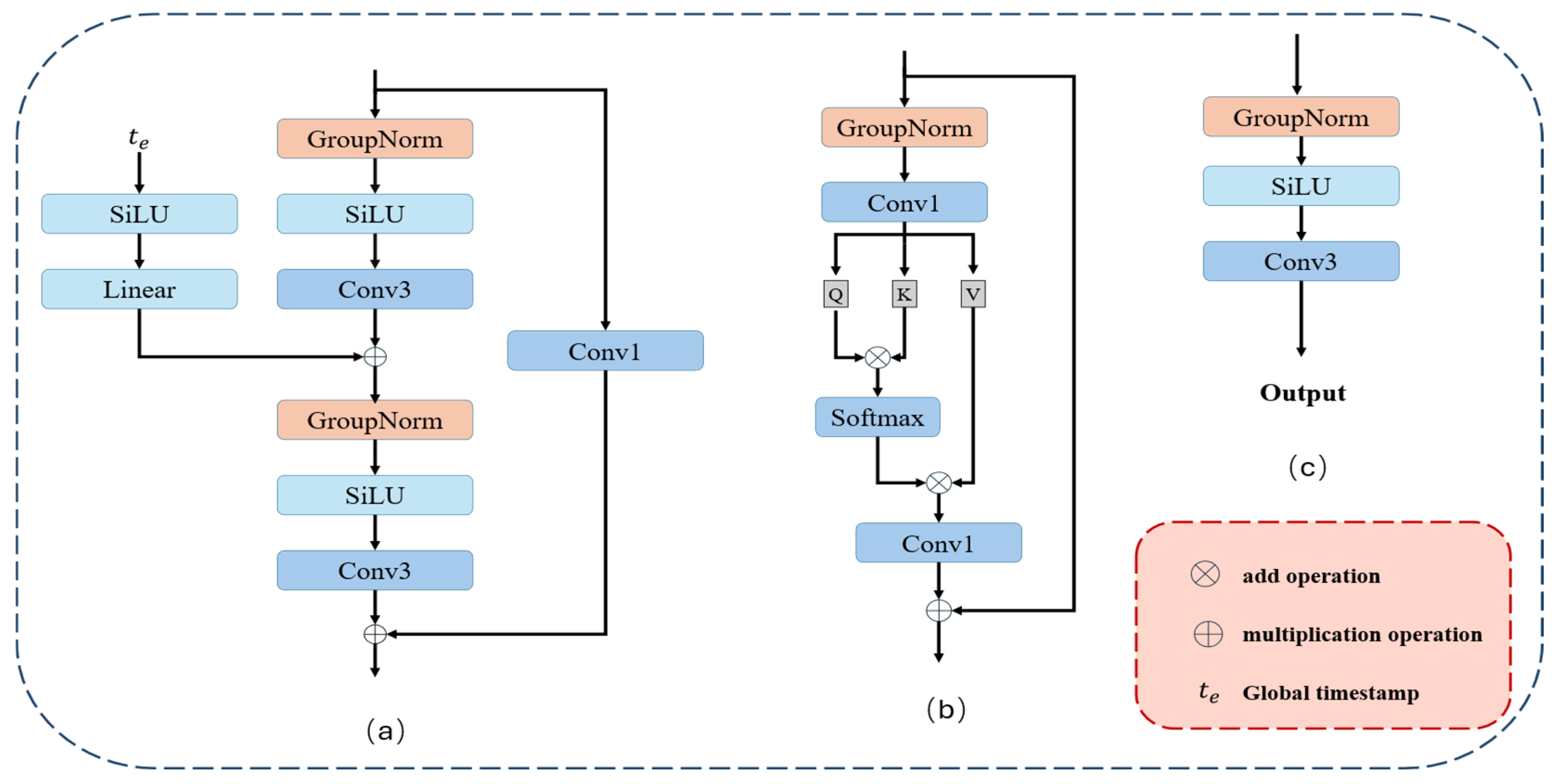
The detailed architectures of the core components in our network—the residual block, self-attention block, and output block—are illustrated in Figure 5. The fundamental feature extraction unit (Figure 5a) is a time-conditional residual block adapted from BigGAN [41], consisting of GN, SiLU activation, and a 3 × 3 convolution. We select GN instead of Batch Normalization (BN) for its better stability in small-batch training, which is typical in the high-noise regime of diffusion models. The SiLU activation is chosen to exploit its self-gating mechanism for improved representational capacity, while its smoothness ensures superior gradient flow compared to ReLU. The timestep $t$ is mapped to a high-dimensional embedding vector $t_e$ using sinusoidal positional encoding. This embedding is then processed and injected into each residual block to provide temporal context regarding the current diffusion stage.

A self-attention block (Figure 5b) is incorporated into the low-resolution bottleneck layers to capture global dependencies. By computing Query (Q), Key (K), and Value (V) matrices, it dynamically enhances the modeling of large-scale structures and textures. Finally, the output block (Figure 5c), comprising GN, SiLU, and a 3 × 3 convolution, is employed in each of the two output branches to predict the noise ${ϵ}_{\theta }$ and variance $v_{\theta }$, respectively.

3.2. Wavelet-Based Downsampling Module

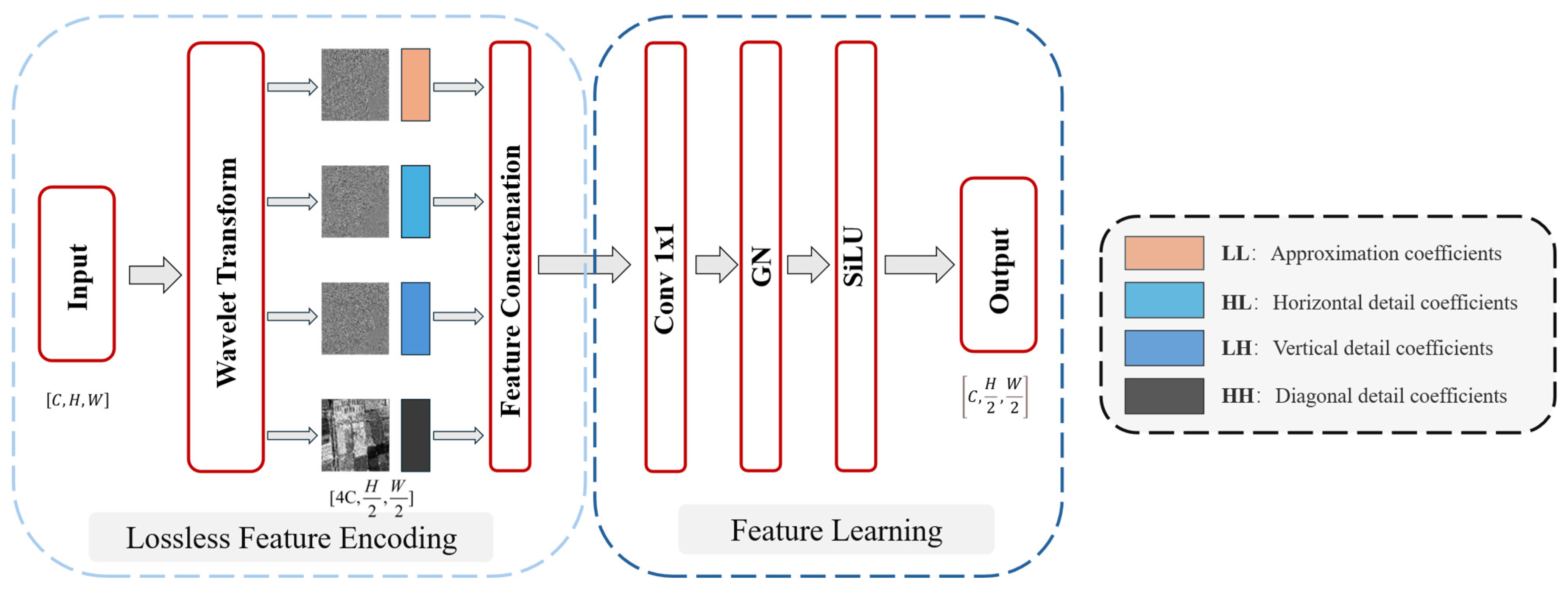
In our proposed network, the downsampling operation within the encoder path is essential for enlarging the receptive field and extracting multi-scale features. Conventional downsampling methods, which typically reduce spatial resolution by discarding or averaging local information, inevitably lead to the loss of fine details in SAR imagery. To mitigate this, we introduce a downsampling module predicated on the 2D Discrete Wavelet Transform (2D-DWT), applied solely during the high-resolution stages of the encoder path. The central tenet of this approach is to transform the challenging task of preserving spatial details into a more tractable problem of differentiating features in the channel domain. Specifically, it is designed to enable the network to distinguish noise-related high-frequency components from those representing terrain features, such as edges and textures. As research by [42] indicates, wavelet-based downsampling significantly enhances the capture and reconstruction of small objects and boundaries. In the context of SAR despeckling, this implies that for minute structures like buildings, well-defined agricultural boundaries, roads, and topographical edges, our wavelet-based downsampling furnishes the network with richer feature information. As depicted in Figure 6, our proposed module is composed of two primary components:

Lossless Feature Encoding Stage: In this stage, the input feature map $X\in {ℝ}^{C\times H\times W}$ undergoes DWT decomposition. We select the Haar wavelet and utilize a symmetric padding mode. This process decomposes $X$ into one low-frequency approximation sub-band $X_{LL}$ (capturing macroscopic structures) and three high-frequency detail sub-bands $X_{HL},X_{LH},X_{HH}$ (encoding horizontal, vertical, and diagonal details, respectively). Subsequently, these four sub-bands are concatenated along the channel dimension to form an information-preserving tensor $X^{\prime }\in {ℝ}^{4C\times {\displaystyle \frac{H}{2}}\times {\displaystyle \frac{W}{2}}}$. This operation, while halving the spatial resolution, transfers the entire spatial information content into the channel dimension. This decomposition method ensures the lossless nature of the feature encoding process, providing an information-rich foundational representation for subsequent multi-scale feature learning. Adaptive Feature Learning: First, the concatenated feature tensor $X^{\prime }$ is fed into a 1 × 1 convolutional layer, whose core function is to adaptively learn the optimal fusion of the low-frequency overview and the multi-directional high-frequency details. Next, a GN layer is employed to stabilize training dynamics and enhance the model’s generalization capability. Finally, the SiLU activation function introduces requisite non-linearity to boost the model’s expressive power. Collectively, this sequence of operations ensures that the module outputs a robust and information-rich multi-scale feature representation, providing a high-quality input for subsequent network layers.

3.3. Efficient Stochastic Sampling

In the domain of unconditional image generation, a series of efficient acceleration paradigms have been proposed to overcome the slow iterative sampling bottleneck of the original DDPM. Among these, Denoising Diffusion Implicit Models (DDIM) [40] stand out as one of the most representative works. The core idea of DDIM is to construct a non-Markovian forward process, which enables the derivation of an equivalent training objective. This, in turn, allows setting the variance of the random term in the reverse process, ${\sigma }_t^2$, to zero. Consequently, the generation process becomes a fully deterministic path, enabling consistent generation from the same noise input to the same image output while substantially reducing the number of sampling steps.

However, for SAR image despeckling, we argue that directly applying DDIM’s deterministic sampling path is suboptimal. A purely deterministic recovery path lacks stochastic exploration capability. When processing complex SAR images, this limitation can result in over-smoothing, loss of critical textures, and edge artifacts, as it fails to flexibly handle the intricate stochastic nature of speckle noise.

Inspired by the “learnable variance” concept introduced by Nichol et al. [39] in generative tasks, we propose an adaptive stochastic denoising path. In our framework, the reverse process variance is dynamically learned by the model from the data, rather than being a fixed hyperparameter. We formulate SAR image despeckling as a conditional generation task, centered on a noise prediction network ${ϵ}_{\theta }\left(x_t,y,t\right)$ conditioned on the noisy image $y$. Unlike standard models, our network not only predicts the noise ${ϵ}_{\theta }$ but also jointly predicts a variance modulation parameter $v_{\theta }$. Our accelerated sampling strategy is implemented as follows:

For a model trained over $T$ steps, we perform inference using a sparse timestep subsequence $\mathcal{S}=\left\{{\tau }_K,{\tau }_{K-1},\dots ,{\tau }_1\right\}$ of length $K$, where $T\ge {\tau }_K>{\tau }_{K-1}>\cdots >{\tau }_1>0$, instead of the full sequence. This subsequence is generated by uniform interval sampling across $\left[1,T\right]$, ensuring representative coverage of the entire diffusion process. For any timestep ${\tau }_i$ in $S$, its cumulative signal coefficient ${\overline{\alpha }}_{{\tau }_i}$ is directly indexed from the pre-computed sequence ${\left\{{\overline{\alpha }}_t\right\}}_{t=1}^T$ of the full $T$ step process. This indexing ensures that the ${\tau }_i$-th step on the sparse path shares the exact Signal-to-Noise Ratio (SNR) characteristics as the ${\tau }_i$-th step on the full path. Based on this, to achieve an effective transition from $x_{{\tau }_i}$ to $x_{{\tau }_{i-1}}$, we re-derive the single-step transition variance ${\beta }_{{\tau }_i}$ and the posterior variance ${\tilde{\beta }}_{{\tau }_i}$:

$${\beta }_{{\tau }_i}=1-{\displaystyle \frac{{\overline{\alpha }}_{{\tau }_i}}{{\overline{\alpha }}_{{\tau }_{i-1}}}}, {\tilde{\beta }}_{{\tau }_i}={\displaystyle \frac{1-{\overline{\alpha }}_{{\tau }_{i-1}}}{1-{\overline{\alpha }}_{{\tau }_i}}}{\beta }_{{\tau }_i}$$

(14)

The above definition ensures that each step along the sparse sampling trajectory strictly adheres to the statistical properties of the original diffusion process. Consequently, the single-step reverse transition from a state $x_{{\tau }_i}$ to its predecessor $x_{{\tau }_{i-1}}$ is implemented by the following reparameterization formula:

$$x_{{\tau }_{i-1}}={\displaystyle \frac{1}{\sqrt{{\alpha }_{{\tau }_i}}}}\left(x_{{\tau }_i}-{\displaystyle \frac{1-{\alpha }_{{\tau }_i}}{\sqrt{1-{\overline{\alpha }}_{{\tau }_i}}}}{ϵ}_{\theta }\left(x_{{\tau }_i},y,{\tau }_i\right)\right)+{\sigma }_{{\tau }_i}z$$

(15)

This transition comprises two components: a deterministic denoising term predicted by the noise estimation network ${ϵ}_{\theta }\left(x_{{\tau }_i},y,{\tau }_i\right)$, and a stochastic noise term ${\sigma }_{{\tau }_i}z$, with $z\sim \mathcal{N}\left(0,I\right)$ representing standard Gaussian noise. The crux of our method lies in dynamically and adaptively modeling the variance ${\sigma }_{{\tau }_i}^2$. Specifically, we parameterize it as a covariance matrix ${\Sigma }_{\theta }\left(x_{{\tau }_i},y,{\tau }_i\right)$, predicted directly by the network as:

$${\Sigma }_{\theta }\left(x_{{\tau }_i},y,{\tau }_i\right)=\exp \left(v_{\theta }\left(x_{{\tau }_i},y,{\tau }_i\right)\cdot \log {\beta }_{{\tau }_i}+\left(1-v_{\theta }\left(x_{{\tau }_i},y,{\tau }_i\right)\right)\cdot \log {\tilde{\beta }}_{{\tau }_i}\right)$$

(16)

This covariance matrix is dynamically interpolated between the theoretical upper bound ${\beta }_{{\tau }_i}$ and lower bound ${\tilde{\beta }}_{{\tau }_i}$ of the variance at timestep ${\tau }_i$. This interpolation is guided by the variance interpolation weight $v_{\theta }\left(x_{{\tau }_i},y,{\tau }_i\right)$, which is predicted concurrently by the network. This adaptive variance mechanism imparts considerable flexibility to the model.

The two acceleration strategies differ fundamentally in their sampling paradigms. DDIM achieves acceleration by introducing a non-Markovian diffusion process, allowing deterministic generative paths and meaningful semantic interpolation in latent space. In contrast, our proposed method retains the intrinsic stochasticity of the Markovian diffusion process, achieving efficiency through adaptive variance prediction and cosine timestep scheduling. This preserves sampling randomness, which is particularly beneficial for addressing complex speckle noise degradation and maintaining structural fidelity in SAR imagery.

3.4. Loss Function

To achieve high-fidelity restoration of SAR images, we formulate a hybrid objective function for our proposed conditional diffusion model. The total objective function, ${\mathcal{L}}_{\mathrm{total}}$, is defined as a weighted sum of two loss terms:

$${\mathcal{L}}_{\mathrm{total}}={\mathcal{L}}_{\mathrm{simple}}+{\lambda }_{\mathrm{vlb}}\cdot {\mathcal{L}}_{\mathrm{vlb}}$$

(17)

Here, ${\mathcal{L}}_{\mathrm{simple}}$ is the primary noise prediction loss, ${\mathcal{L}}_{\mathrm{vlb}}$ is the variational lower bound (VLB) loss, and ${\lambda }_{\mathrm{vlb}}$ is a weighting coefficient that balances their contributions. ${\mathcal{L}}_{\mathrm{simple}}$ guides ${\mathsf{ϵ}}_{\theta }$ to predict the Gaussian noise $ϵ$ at timestep $t$ using MSE loss.

$${\mathcal{L}}_{\mathrm{simple}}={\mathbb{E}}_{t,x_0,\mathsf{ϵ},y}\left[{\parallel \mathsf{ϵ}-{\mathsf{ϵ}}_{\theta }\left(x_t,t,y\right)\parallel }^2\right]$$

(18)

In this equation, $t\in \left\{1,\dots ,T\right\}$ is a uniformly sampled timestep and $\mathsf{ϵ}\sim \mathcal{N}\left(\mathbf{0},I\right)$ is standard Gaussian noise. To enable the model to learn the reverse process variance ${\Sigma }_{\theta }\left(x_t,t,y\right)$, we introduce the variational lower bound loss term ${\mathcal{L}}_{\mathrm{vlb}}$. This term is formulated by minimizing the KL divergence between the “true” reverse posterior distribution $q\left(x_{t-1}|x_t,x_0\right)$ and the model-parameterized distribution $p_{\theta }\left(x_{t-1}|x_t,y\right)$:

$${\mathcal{L}}_{\mathrm{vlb}}={\mathbb{E}}_{t,x_0,y}\left[D_{\mathrm{KL}}\left(q\left(x_{t-1}|x_t,x_0\right)\parallel p_{\theta }\left(x_{t-1}|x_t,y\right)\right)\right]$$

(19)

The magnitude of the VLB loss, ${\mathcal{L}}_{\mathrm{vlb}}$, is intrinsically tied to the discretization granularity of the diffusion process (i.e., the total number of steps $T$). To mitigate potential gradient imbalance, we propose a scale-normalized weighting strategy:

$${\lambda }_{\mathrm{vlb}}={\displaystyle \frac{T}{1000}}$$

(20)

This strategy linearly scales the weight ${\mathcal{L}}_{\mathrm{vlb}}$ with $T$, ensuring stable gradient contributions from ${\mathcal{L}}_{\mathrm{vlb}}$ across different $T$ configurations and facilitating robust variance learning. For the $T=1000$ setup used in our study, this yields ${\lambda }_{\mathrm{vlb}}=1.0$.

4. Experiments and Results

4.1. Datasets

To enhance the model’s adaptability to diverse terrain types and complex scenarios, we constructed the Multi-Scene SAR Synthetic Dataset (MS-SAR) by selecting representative scenes—urban, mountainous, and agricultural—from the DSIFN [43] and Sentinel-2 [44] optical datasets. We generated noise samples corresponding to different ENLs ($L = 1, 2, 4$) to simulate varied imaging conditions. Each sample pair consists of a noisy SAR-simulated image (input) and a clean optical image (ground truth), with all patches uniformly cropped to $256\times 256$ pixels. The dataset is partitioned into training (3000 pairs), validation (200 pairs), and test sets (100 pairs), ensuring balanced representation across all representative scenes in each subset.

Despite the convenience of optical-based synthetic data for supervised training of SAR despeckling models, a fundamental limitation remains: the domain gap between optical and real SAR data. This gap arises from fundamentally different imaging physics—optical imaging relies on passive spectral reflectance, while SAR relies on active microwave backscattering—resulting in systematic biases in texture and structural representations between synthetic and real SAR data [45]. To bridge this gap, we utilized a multi-temporal real SAR dataset for fine-tuning, derived from Sentinel-1 C-band Ground Range Detected (GRD) products. This dataset includes 10 co-registered VV-polarized Interferometric Wide (IW) swath images covering the Toronto region in Canada, with a spatial resolution of $5 \mathrm{m}\times 20 \mathrm{m}$. A pseudo-noise-free reference image was generated via multi-temporal averaging, using a single-date image (5 September 2022) as the noisy input paired with the fused reference as the supervised ground truth [46]. This pair was cropped into 1000 $256\times 256$ patches for training. Additionally, we incorporated Sentinel-1A Single Look Complex (SLC) products for testing, encompassing diverse terrains including urban, mountainous, rural, and agricultural areas in Beijing, China, and Toronto, Canada. These data were acquired in IW mode with VV polarization and a spatial resolution of $3 \mathrm{m}\times 15 \mathrm{m}$.

4.2. Experiments Preparation

All deep learning experiments in this study were conducted on an NVIDIA A800 80 GB PCIe GPU, running on the Ubuntu operating system. The implementations were developed in Python 3.8 using the PyTorch 1.8.0 deep learning framework. For model training, we utilized the AdamW optimizer with momentum coefficients ${\beta }_1=0.9$ and ${\beta }_2=0.999$. The initial learning rate was set to ${\eta }_0=5\times {10}^{-5}$, with the learning rate scheduled using the Cosine Annealing with Warm Restarts strategy. The initial restart period was $T_0=20$ epochs, with subsequent periods scaled by a multiplicative factor $T_{\mathrm{mult}}=2$, and the minimum learning rate set to ${\eta }_{\min }=1\times {10}^{-6}$. Training was conducted for a total of 400 epochs. The diffusion process was configured with 1000 timesteps, employing a cosine noise schedule where the noise variance ${\beta }_t$ ranged from $1\times {10}^{-6}$ to $1\times {10}^{-2}$. The model was first trained for 300 epochs on a synthetic dataset derived from optical images, using a batch size of 16. Subsequently, fine-tuning was performed for 100 epochs on a multi-temporal SAR dataset constructed from real SAR images, with a batch size of 8. During inference, we applied the same cosine noise schedule and used 50 sampling timesteps to generate the final results of the proposed method.

4.3. Methods for Comparison

To validate the reliability and effectiveness of the proposed method, we conducted comprehensive comparisons with seven established SAR image despeckling methods: PPB, BM3D, SAR-CNN, SAR-DRN, SAR-Trans, SAR-ON [47], SAR-CAM, and SAR-DDPM. Among these, PPB and BM3D are classical non-local approaches. For PPB, we used a patch size of $7\times 7$ pixels and a search range of $21\times 21$ pixels. For BM3D, block-matching was performed with a block size of $12\times 12$ pixels and a stride of 2 pixels, while the search window for similar blocks was set to $39\times 39$ pixels. The remaining methods are neural network-based. SAR-CNN, SAR-DRN, and SAR-ON are based on convolutional neural networks (CNNs). SAR-CAM employs successive attention blocks concatenated to progressively extract features. SAR-Trans utilizes a hierarchical encoder based on the Pyramid Vision Transformer architecture for multi-scale feature extraction. In contrast to SAR-DDPM, which relies on a standard 1000-timestep sampling procedure, our proposed method achieves significant computational efficiency gains by reducing the sampling steps to only 50 during inference, while preserving superior despeckling performance.

4.4. Experimental Results on Synthetic Datasets

To comprehensively evaluate the performance of the proposed method, detailed experimental verification was conducted on the MS-SAR dataset, encompassing three typical land-cover scenes (urban, mountainous, and farmland) under different numbers of looks ($L = 1, 2, 4$). The peak signal-to-noise ratio (PSNR) and structural similarity index measure (SSIM) were employed as objective evaluation metrics. Specifically, PSNR quantitatively assesses despeckling performance by calculating the mean squared error between reconstructed and reference images, expressed in decibels (dB), where higher values indicate superior denoising quality. SSIM comprehensively evaluates luminance, contrast, and structural similarity, ranging from 0 to 1, with values closer to 1 indicating higher structural fidelity. Additionally, qualitative visual analyses were performed to verify the balance achieved by each method between detail preservation and noise suppression.

Table 1. Quantitative results on the MS-SAR dataset. Bold denotes the best result for each scene within the same look number.

Look	Algorithm	City		Farm		Mountain
		SSIM	PSNR	SSIM	PSNR	SSIM	PSNR
1-look	PPB	0.683	20.84	0.720	21.48	0.673	21.03
	BM3D	0.725	21.79	0.734	23.42	0.734	22.97
	SAR-DRN	0.713	21.43	0.754	23.21	0.736	21.93
	SAR-Trans	0.741	22.46	0.770	25.15	0.770	23.78
	SAR-ON	0.742	23.76	0.795	25.46	0.787	24.54
	SAR-CAM	0.758	23.84	0.788	25.41	0.776	24.75
	SAR-DDPM	0.750	23.85	0.806	26.07	0.788	24.31
	Proposed	0.764	24.68	0.824	26.86	0.795	25.89
2-look	PPB	0.728	21.25	0.819	22.34	0.803	22.48
	BM3D	0.763	23.41	0.837	24.68	0.828	23.89
	SAR-DRN	0.766	22.78	0.827	24.78	0.824	23.61
	SAR-Trans	0.775	23.85	0.844	26.78	0.808	25.12
	SAR-ON	0.781	25.18	0.858	26.95	0.846	25.68
	SAR-CAM	0.795	25.22	0.864	26.84	0.855	25.94
	SAR-DDPM	0.837	25.34	0.864	27.81	0.860	25.34
	Proposed	0.842	26.01	0.870	28.56	0.864	26.12
4-look	PPB	0.808	24.25	0.849	24.84	0.823	24.48
	BM3D	0.843	25.11	0.867	26.07	0.858	25.23
	SAR-DRN	0.846	24.78	0.847	26.78	0.824	25.61
	SAR-Trans	0.850	25.24	0.864	28.41	0.877	26.46
	SAR-ON	0.859	26.68	0.891	28.89	0.885	27.16
	SAR-CAM	0.852	26.72	0.881	29.05	0.890	27.13
	SAR-DDPM	0.857	26.78	0.904	29.13	0.886	27.34
	Proposed	0.863	27.43	0.910	30.56	0.894	28.06

presents the quantitative evaluation results on the MS-SAR dataset, providing a comprehensive comparative analysis with seven state-of-the-art SAR despeckling algorithms. Optimal results are highlighted in bold. Traditional algorithms (PPB and BM3D) exhibit significantly inferior performance under single-look conditions. Among the deep learning-based methods, SAR-Trans performs notably well in farmland scenes but shows limited adaptability to complex structural textures, indicating strong scene dependency. SAR-ON and SAR-CAM demonstrate relatively balanced cross-scene generalization capability, occasionally surpassing the baseline diffusion model SAR-DDPM under certain conditions. In contrast, the proposed method consistently achieves the best performance across all test scenarios and look-number conditions, delivering average performance gains of 0.67–1.43 dB in PSNR and 0.01–0.06 in SSIM compared to the second-best baseline model.

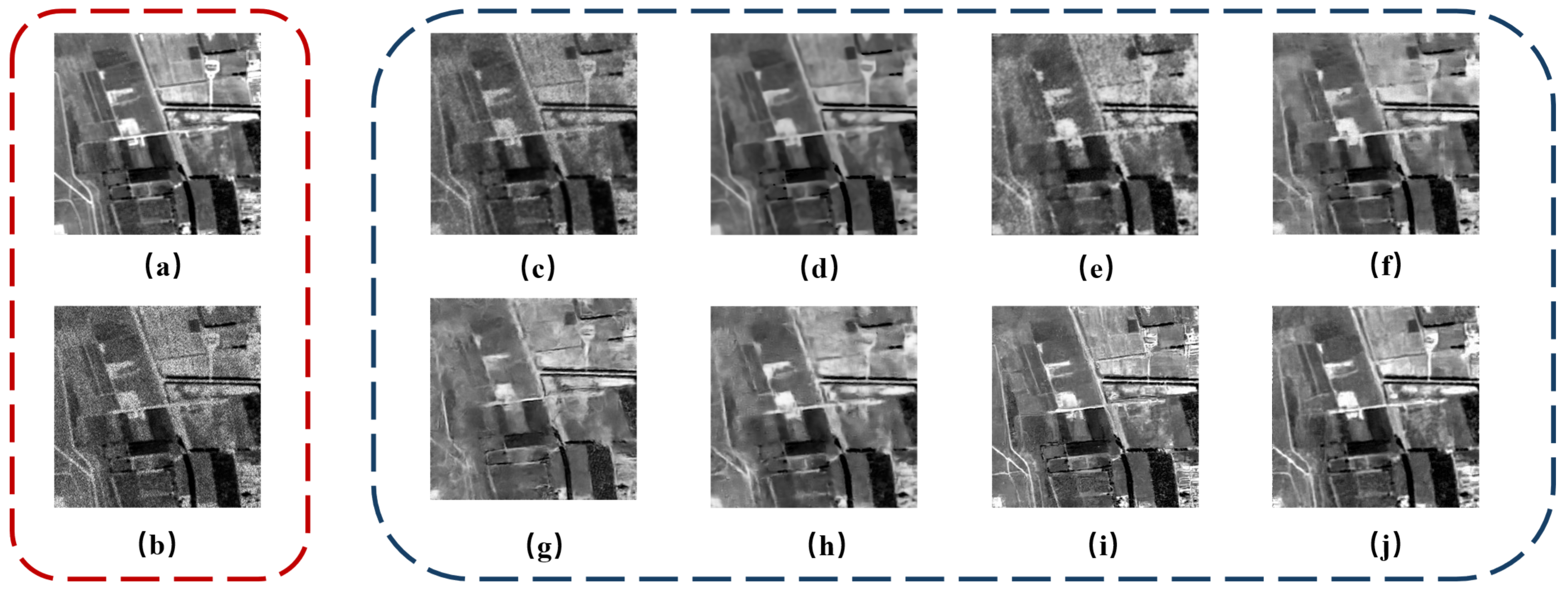
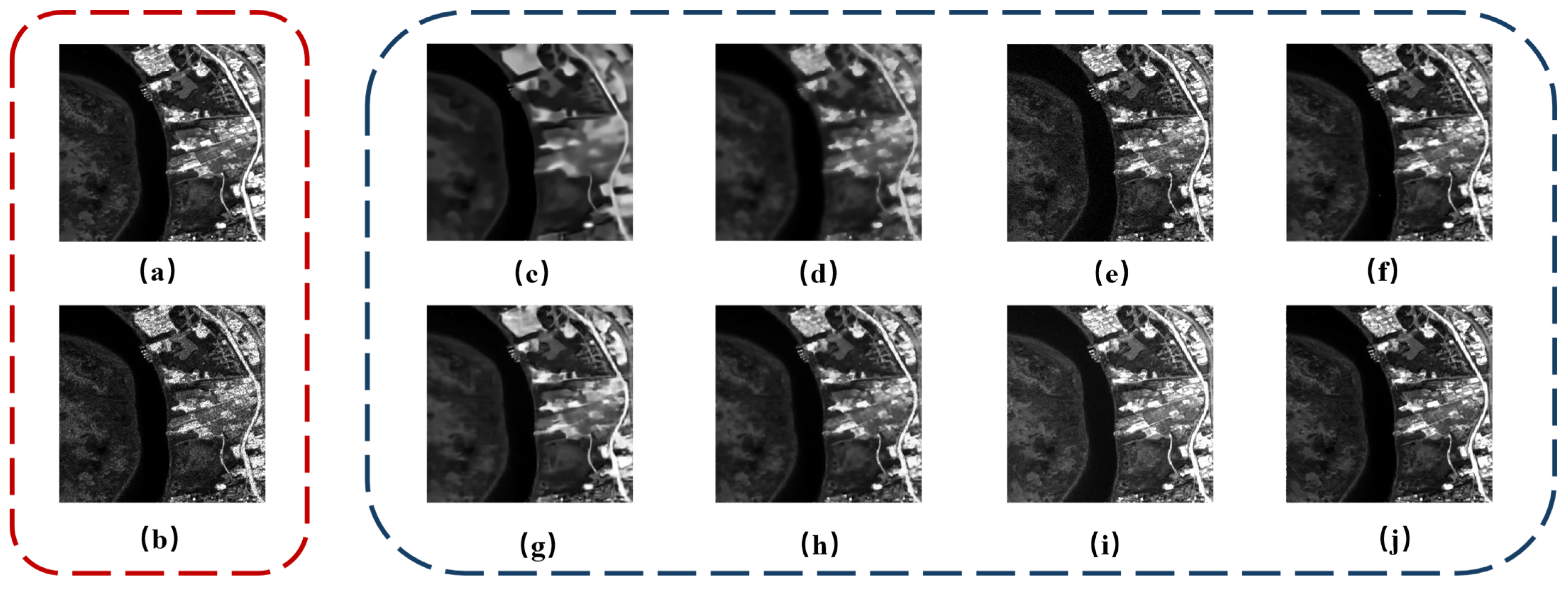
The imaging results under single-look conditions are shown in Figure 7, where the original images are severely degraded by speckle noise. While the traditional algorithms PPB and SAR-BM3D exhibit some noise suppression capabilities, they suffer from over-smoothing and detail loss, respectively. Among the deep learning methods, SAR-DRN shows prominent residual noise artifacts; SAR-Trans, SAR-CAM, and SAR-ON display mild blurring in complex textured regions; and SAR-DDPM demonstrates strong edge preservation and noise suppression but falls short in detail recovery and structural fidelity. In contrast, our proposed method achieves superior noise suppression while effectively preserving edge information and textural details. 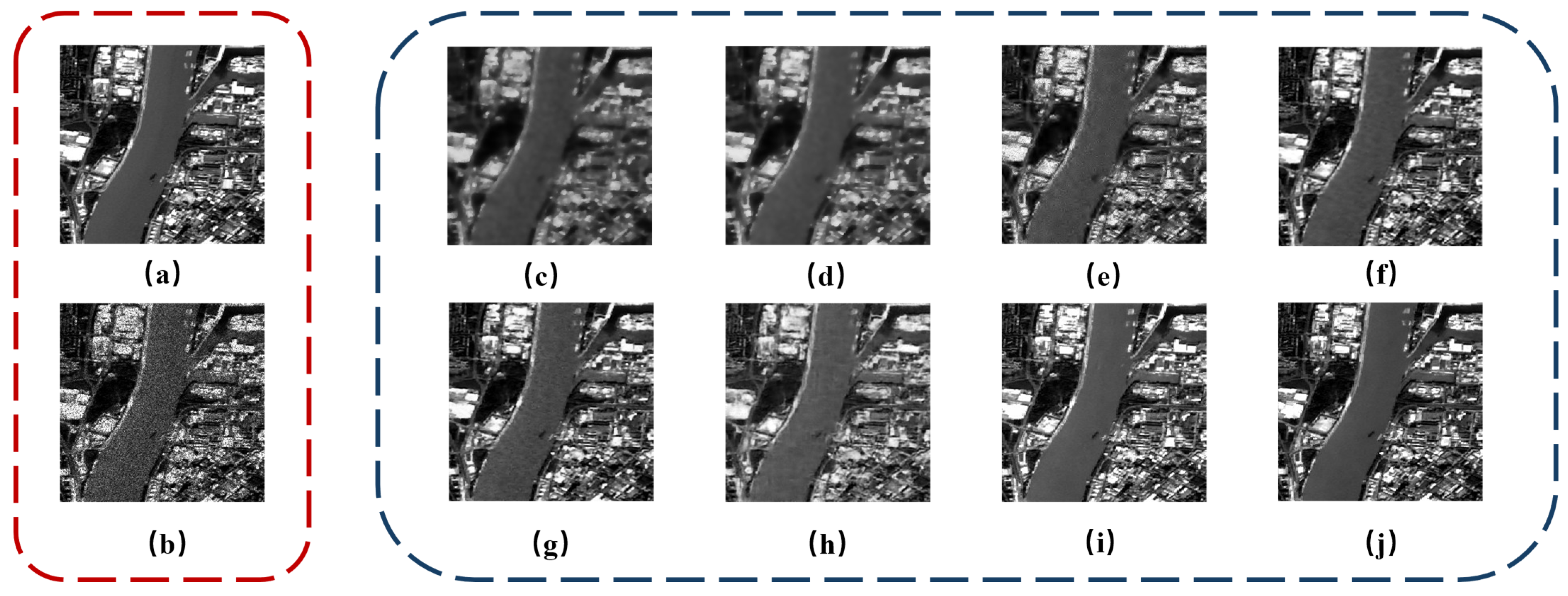The results for 2-look processing are shown in Figure 8. Although PPB and BM3D maintain adequate noise suppression, the over-smoothing issue persists, resulting in loss of structural details. SAR-DRN, SAR-Trans, and SAR-ON exhibit limited recovery capabilities in complex urban areas. Our proposed method attains optimal noise suppression alongside superior restoration of urban structures. Under the 4-look conditions illustrated in Figure 9, the noise level is further reduced, and all methods show markedly improved despeckling performance, though differences remain evident. SAR-DRN and SAR-CAM produce noticeable artifacts in densely built-up areas, degrading image quality. SAR-Trans and SAR-ON exhibit over-smoothing, leading to partial loss of structural details. While SAR-DDPM offers reasonable noise suppression, it is affected by intensity biases. Our proposed method effectively suppresses noise while optimally preserving building contours, demonstrating exceptional structural fidelity.

In summary, the comparative results against traditional methods and multiple baselines indicate that our method holds significant advantages in edge preservation, structural integrity, and recovery of complex textural details.

4.5. Experimental Results on Real SAR Datasets

To further validate the effectiveness and generalization capability of the proposed method in real-world scenarios, both the proposed and comparative methods were evaluated on various scenes within a real SAR image test set. This section presents the experimental results for farmland, urban, and mountainous areas, aiming to assess each algorithm’s despeckling performance across homogeneous, heterogeneous, and strongly heterogeneous regions in SAR images. Evaluations include both subjective visual assessments and objective quantitative metrics.

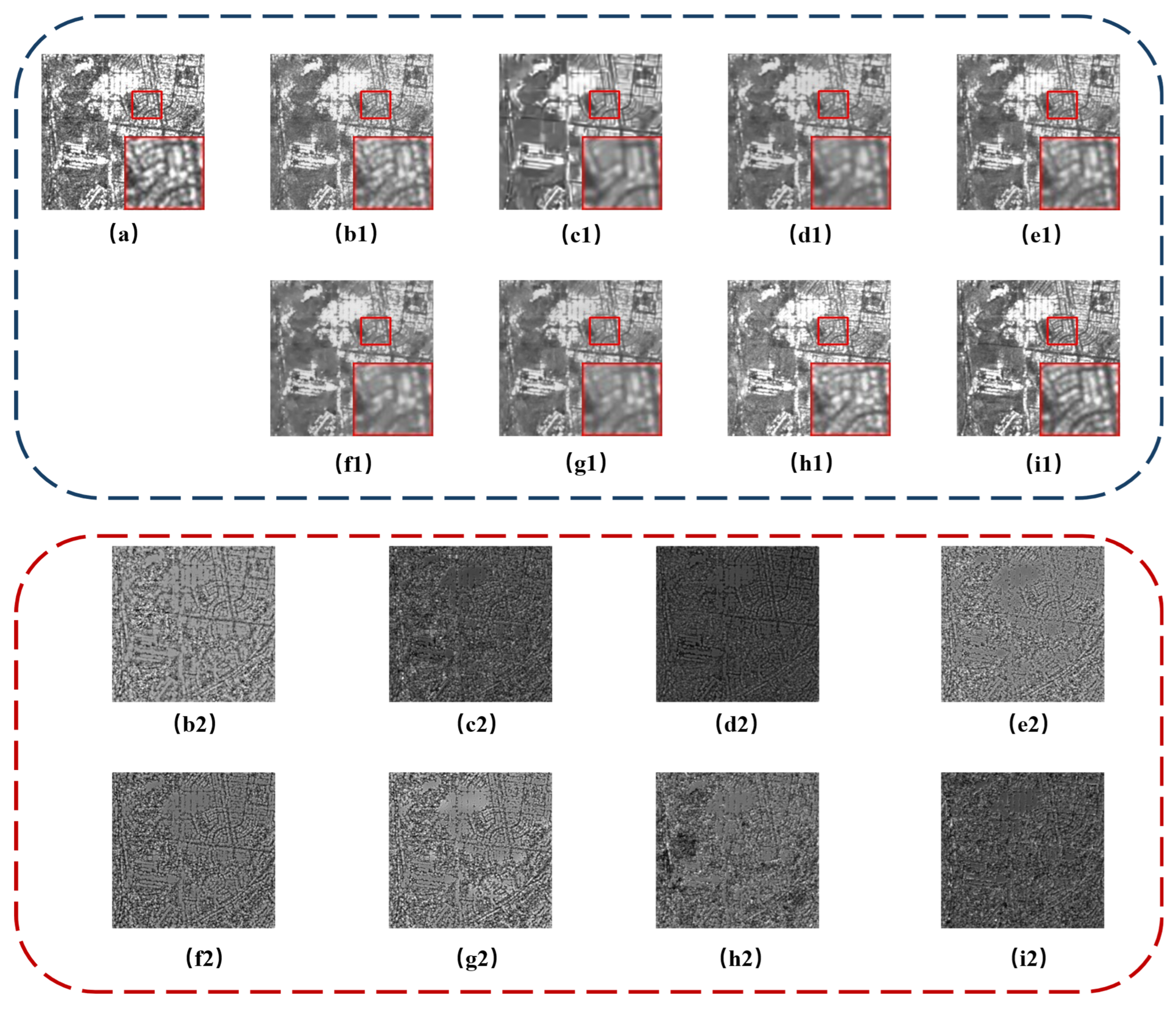
The experimental evaluation was conducted on a complex SAR urban image encompassing building clusters, road networks, and homogeneous areas, with despeckling results visualized in Figure 10. PPB provides insufficient noise suppression in urban scenes, retaining noticeable granular artifacts, as evidenced by substantial textural residues in its ratio image; SAR-BM3D induces over-smoothing, severely blurring architectural contours and road boundaries. Deep learning-based methods, while improved, retain shortcomings: SAR-DRN and SAR-Trans enhance background noise suppression but introduce subtle halo artifacts, with their residual maps showing evident edge remnants; SAR-ON and SAR-CAM perform well in strong scattering regions yet inadequately preserve fine details; SAR-DDPM demonstrates robust denoising but generates textural artifacts in homogeneous areas, with its ratio image revealing mismatches between the generated prior and actual speckle statistics. In contrast, our proposed method achieves superior despeckling across complex urban road networks and homogeneous regions, while faithfully preserving key geometric structures and radiometric characteristics.

The experimental results for the mountainous scene are presented in Figure 11. This scene is characterized by rich topographic details, including steep ridges and smooth slope faces. Consistent with the findings in urban areas, traditional filtering algorithms struggle to achieve an optimal balance between noise suppression and structural fidelity. Specifically, SAR-DRN, SAR-Trans, and SAR-ON exhibit over-smoothing in extensive slope areas, resulting in markedly softened ridge lines, reduced contrast in subtle gullies, and diminished topographic relief. Their corresponding residual maps reveal prominent ridge contours, indicating a systematic radiometric bias in the signal-noise separation process, whereby essential topographic gradient information is mistakenly categorized as noise. Although SAR-CAM and SAR-DDPM yield relatively superior despeckling outcomes, their residual maps still exhibit faint but discernible structural leakage. In stark contrast, our method’s superiority is evident: it preserves key topographical features without artifacts, leaving a residual map that is virtually free of structural leakage.

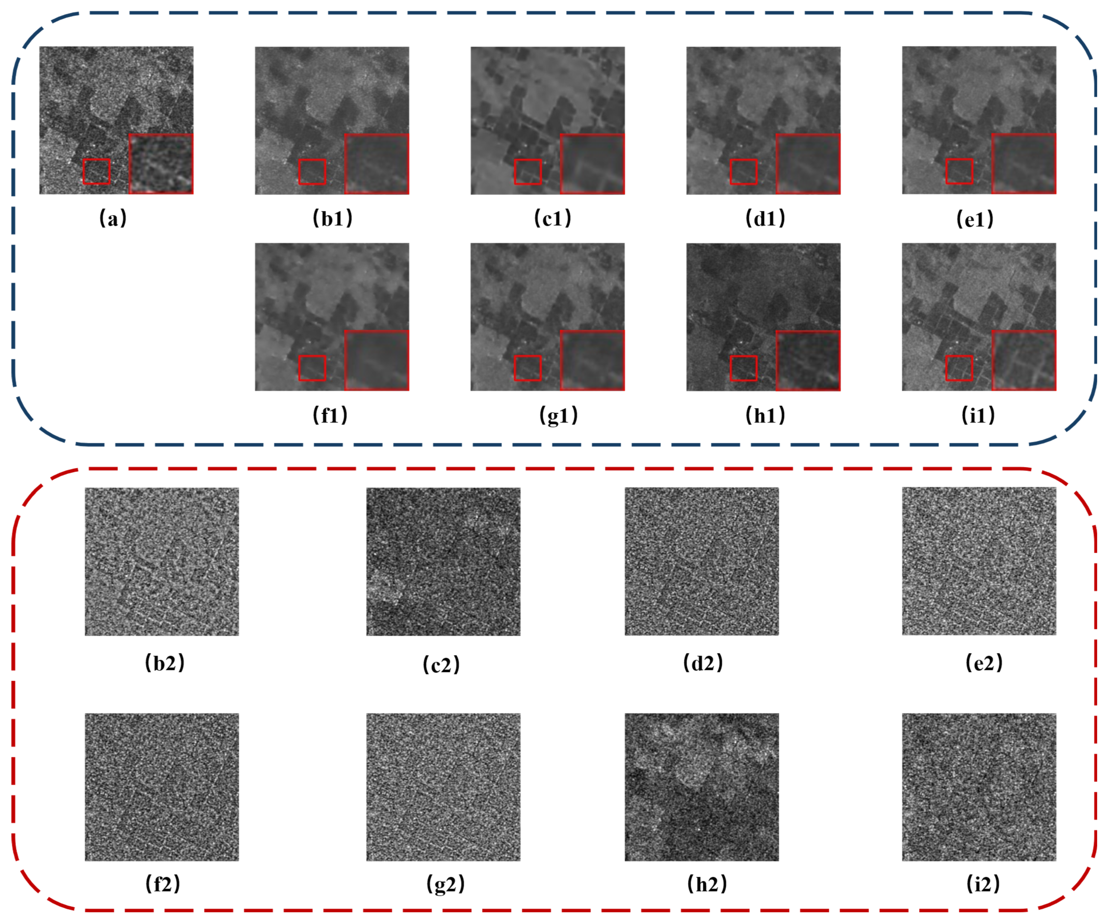
The farmland scene results in Figure 12 clearly reveal the inherent limitations of conventional methods: the PPB algorithm leaves significant granular artifacts in the processed image, while SAR-BM3D causes severe over-smoothing. CNN-, attention-, and Transformer-based models all fail to effectively decouple the clean signal from the observed speckle, with their residual maps showing prevalent structural remnants—particularly linear traces along farmland boundaries—manifesting as varying degrees of over-smoothing. As the baseline, SAR-DDPM introduces pronounced brightness shifting in homogeneous regions, with its ratio map exhibiting significant structural remnants that confirm systematic bias in the despeckling process, severely compromising radiometric reliability. In contrast, our proposed method delivers artifact-free smoothing in homogeneous regions while preserving sharp edges and strong scatterers. Its ratio map most closely approximates the ideal random speckle field among deep learning approaches, providing compelling evidence of its superior despeckling performance.

To objectively quantify the qualitative observations, we performed quantitative evaluations on despeckling results across three typical scenarios, with the best method in red bold and the second-best in red italics, as shown in

Table 2. Comparative evaluation of SAR image despeckling algorithms on real-world scenarios. The best and second-best results under different scenarios are highlighted in bold and italics, respectively.

Scene	Algorithm	ENL	MOI	MOR	EPD-ROA Vert	EPD-ROA Hori	M-Index
City	PPB	128.15	1.0876	0.9057	0.9017	0.8794	6.865
	SAR-BM3D	148.35	0.9543	1.0456	0.9432	0.9018	4.325
	SAR-DRN	142.24	0.9243	1.0765	0.9445	0.8964	5.765
	SAR-CAM	206.76	0.9714	1.0235	0.9846	0.9832	3.636
	SAR-Trans	126.65	0.9504	1.0345	0.9438	0.9217	2.993
	SAR-ON	132.28	0.9813	1.0143	0.9849	0.9846	3.778
	SAR-DDPM	127.66	0.9746	1.0173	0.9882	0.9887	2.874
	Proposed	149.37	0.9832	1.0104	0.9923	0.9918	2.335
Mountain	PPB	134.19	0.8973	1.1293	0.8817	0.8457	8.327
	SAR-BM3D	76.14	0.9297	1.0734	0.9015	0.8582	7.689
	SAR-DRN	83.54	0.8752	1.1293	0.9015	0.8631	5.793
	SAR-CAM	107.37	0.9453	1.0548	0.9015	0.8734	4.038
	SAR-Trans	154.37	0.9478	1.0473	0.9166	0.8951	4.732
	SAR-ON	137.80	0.9615	0.9814	0.9177	0.8793	3.487
	SAR-DDPM	116.72	1.0464	0.9966	0.9203	0.8843	3.019
	Proposed	128.47	0.9789	1.0104	0.9278	0.9014	2.866
Farm	PPB	317.41	0.9345	0.9256	0.9211	0.8945	7.922
	SAR-BM3D	325.29	0.9546	1.0597	0.9545	0.9247	4.472
	SAR-DRN	164.86	0.9674	1.0349	0.9458	0.9228	5.233
	SAR-CAM	272.99	0.9728	1.0288	0.9766	0.9874	3.452
	SAR-Trans	243.64	0.9765	1.0243	0.9594	0.9489	6.768
	SAR-ON	340.02	0.9828	1.0148	0.9885	0.9842	3.019
	SAR-DDPM	273.67	0.8407	1.2793	0.9884	0.9887	4.273
	Proposed	318.91	1.0126	0.9885	0.9927	0.9908	2.986

. Due to the lack of noise-free references for real SAR images, we adopted a four-dimensional no-reference framework assessing performance in speckle suppression, radiometric fidelity, edge preservation, and overall quality. The Equivalent Number of Looks (ENL) quantifies speckle suppression via the squared mean-to-variance ratio in homogeneous regions [48]; higher ENL indicates better suppression. Radiometric fidelity is assessed using Mean of Image (MOI) and Mean of Ratio (MOR) [49]: MOI evaluates bias via pre- and post-despeckling mean ratios in homogeneous regions, while MOR detects distortion through ratio image means. We analyzed 5 regions of interest per image; ideally, MOI and MOR approach 1, with deviations signaling bias [50]. The Edge Preservation Degree based on Ratio of Averages (EPD-ROA) [51] measures structural consistency via local mean ratios pre- and post-filtering, including vertical and horizontal components; values near 1 denote better edge/detail preservation. The M-index [52] combines first-order (speckle suppression, mean preservation) and second-order (structure preservation) residuals for a holistic score; values near 0 indicate optimal balance between suppression and preservation.

Analysis of the quantitative results from Table 2 yields the following conclusions:

Urban Scene: In the urban scene, characterized by the highest structural complexity, our proposed method attains the lowest M-index (2.3356), underscoring its superior overall performance. This aligns closely with the visual observations of sharp building contours and clear road boundaries. Regarding radiometric fidelity, our method’s MOI (0.9832) and MOR (1.0104) are remarkably close to the ideal value of 1, quantitatively confirming its efficacy in alleviating radiometric distortions common in methods like SAR-DDPM and SAR-Trans. Although SAR-CAM achieves the highest ENL (206.76), indicating strong smoothing capability, its suboptimal EPD-ROA score reflects a compromise in structural detail preservation.

Mountainous Scene: In the mountainous scene, SAR-Trans secures the second-best ENL and EPD-ROA, yet its M-index is outperformed by our method. Our approach achieves the optimal M-index (2.8668) and EPD-ROA, demonstrating adaptability to heterogeneous terrains. Moreover, it exhibits robust radiometric fidelity (MOI = 0.9789, MOR = 1.0104), surpassing the notable biases in baselines such as SAR-DDPM (MOI = 1.0764).

Farmland Scene: In the farmland scene, dominated by large homogeneous regions, the key differentiators among methods are radiometric fidelity and overall performance. While SAR-ON and SAR-BM3D marginally surpass our method in ENL, our approach excels in other metrics and secures the lowest M-index (2.986). Additionally, its MOI (1.0126) and MOR (0.9885) closely approximate the ideal value of 1, mitigating the radiometric shifts prevalent in baselines like SAR-DDPM.

In conclusion, a comprehensive quantitative evaluation across three typical land-cover types reveals that our proposed method consistently achieves optimal or near-optimal performance on key metrics. This not only quantitatively validates the method’s robustness but also elucidates its core advantage: efficiently suppressing speckle noise in SAR images while preserving the fidelity of complex structures (e.g., edges and textures) and maintaining radiometric accuracy.

5. Discussion

5.1. Ablation Study

To validate the effectiveness of key components in our diffusion-based network, we conducted ablation studies to quantitatively assess the contributions of the wavelet-based downsampling module and joint noise-variance prediction. Forty images with $L = 1, 2, 4$ were randomly selected from the MS-SAR test set, with results summarized in

Table 3. Quantitative evaluation of ablation studies. The best results are highlighted in bold.

Experiment	Wavelet Basis	Prediction Mode	L = 1 (PSNR/SSIM)	L = 2 (PSNR/SSIM)	L = 4 (PSNR/SSIM)	Single-Step Inference Time (s)
Experiment 1	None	${ϵ}_{\theta }$	25.43/0.762	27.58/0.792	29.40/0.834	0.03473
Experiment 2	None	${ϵ}_{\theta }+v_{\theta }$	25.84/0.788	27.99/0.816	29.71/0.858	0.03478
Experiment 3	Haar	${ϵ}_{\theta }+v_{\theta }$	26.32/0.817	28.47/0.843	30.29/0.883	0.03468
Experiment 4	db4	${ϵ}_{\theta }+v_{\theta }$	26.23/0.804	28.38/0.834	30.20/0.874	0.03474
Experiment 5	bior2.2	${ϵ}_{\theta }+v_{\theta }$	25.47/0.782	27.62/0.810	29.44/0.852	0.03486

.

To assess the joint prediction strategy (${ϵ}_{\theta }+v_{\theta }$), we compared Experiment 1 (predicting only ${ϵ}_{\theta }$) with Experiment 2. Across degradation levels, Experiment 2′s PSNR and SSIM consistently exceed Experiment 1′s, confirming that simultaneous v_\theta prediction improves reconstruction stability and precision.

To verify the wavelet-based module’s contribution, we compared Experiment 3 (Haar wavelet downsampling) against Experiment 2 (conventional strided convolution). Experiment 3 outperforms Experiment 2 across all noise levels, validating that our lossless module preserves high-frequency information for decoupled multi-scale representations, enhancing despeckling performance and structural fidelity. Inference times between Experiments 3 and 2 show no perceptible overhead, confirming the module’s efficiency and plug-and-play nature.

Comparing Experiments 3–5 reveals the Haar wavelet’s superior performance across all look conditions over db4 and bior2.2. Haar’s advantages include integer coefficients preventing floating-point errors, minimal support length (L = 2) reducing boundary effects, and strict orthogonality ensuring energy conservation—aligning well with diffusion models’ probabilistic framework [53]. This suggests prioritizing numerical compatibility over approximation accuracy when selecting wavelets for deep generative models.

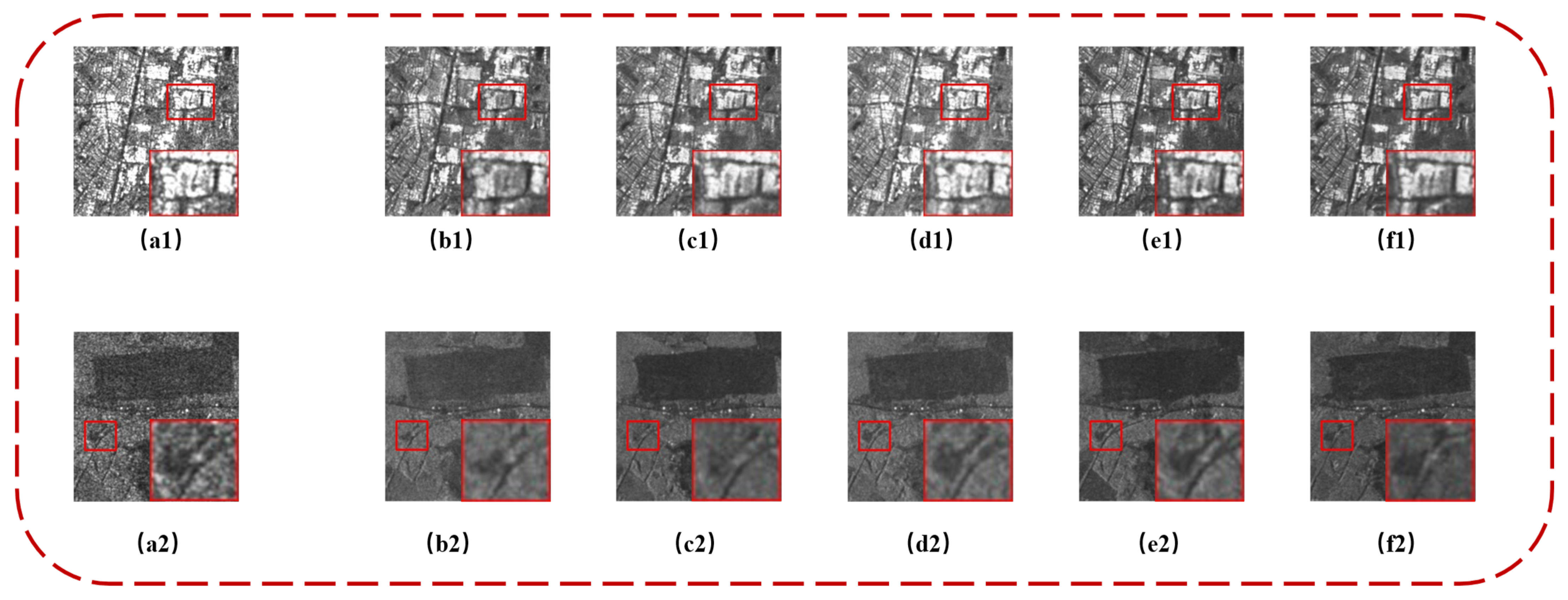
For comprehensive evaluation, we conducted visual quality assessments on the real SAR test dataset (Figure 13). Comparing baseline (Experiment 1) with joint prediction (Experiment 2) shows improvements in building contours and strong scatterer fidelity; rural ridge and road boundaries also exhibit greater clarity, verifying the strategy’s effectiveness. Introducing wavelet downsampling (Experiments 3–5) further enhances despeckling quality and edge preservation. Relative to minor edge-rounding or blurring in Daubechies-4 (Experiment 4) and Biorthogonal-2.2 (Experiment 5), Haar (Experiment 3) excels in reconstructing orthogonal buildings, linear features, and subtle terrain boundaries in rural scenes.

In summary, the visual evidence aligns with Table 3’s quantitative analyses, demonstrating our method’s state-of-the-art performance in efficient SAR despeckling with superior structural fidelity.

5.2. Sampling Strategy Analysis

Although iterative sampling is foundational to diffusion models for achieving high-fidelity generation, the typical reverse sampling process involving thousands of steps (T = 1000) incurs substantial inference latency. This section systematically evaluates the denoising performance of our proposed efficient reverse sampling strategy against DDIM across various sampling steps. We conducted rigorous quantitative and qualitative experiments to elucidate the fundamental differences in efficiency, performance, and robustness among different sampling strategies.

Table 4. Comparison of inference performance across multiple sampling steps for different samplers. The best results are highlighted in bold.

Sampler	Metric	t = 1000	t = 750	t = 500	t = 250	t = 100	t = 50	t = 25	t = 10	t = 5
DDPM	SSIM	0.748	-	-	-	-	-	-	-	-
	PSNR (dB)	25.08	-	-	-	-	-	-	-	-
	Time (s)	34.69	-	-	-	-	-	-	-	-
DDIM	SSIM	-	0.631	0.584	0.566	0.743	0.762	0.771	0.542	0.691
	PSNR (dB)	-	21.21	19.21	20.47	22.17	23.29	23.45	18.82	22.6
	Time (s)	-	26.69	17.58	8.87	3.52	1.78	0.88	0.36	0.19
Proposed	SSIM	-	0.743	0.751	0.763	0.795	0.784	0.786	0.765	0.694
	PSNR (dB)	-	25.02	25.12	25.34	25.46	25.53	25.29	25.02	19.28
	Time (s)	-	26.14	17.49	8.64	3.49	1.73	0.87	0.35	0.18

illustrates a detailed comparison of inference performance across multiple sampling steps (t) for different samplers. Experimental results clearly demonstrate that our proposed method effectively overcomes the inherent trade-off between inference efficiency and generation quality in SAR image denoising tasks. Compared to the DDPM baseline employing the complete 1000-step sampling process (taking 34.69 s), our method dramatically reduces inference time to 0.87 s at just 25 sampling steps (t = 25), achieving nearly a 40-fold theoretical acceleration. Crucially, despite this significant acceleration, performance metrics were not compromised but instead surpassed those of the baseline model.

Moreover, in horizontal comparisons against the widely adopted accelerated sampler DDIM, our method consistently exhibited comprehensive and stable performance advantages across all evaluated sampling steps under comparable computational costs. Furthermore, our proposed method demonstrated exceptional robustness across a broad and practically significant acceleration interval (t = 250 to t = 25), maintaining superior performance metrics in stark contrast to DDIM.

To complement the quantitative analysis, Figure 14 and Figure 15 visually illustrate the despeckling results of the two acceleration strategies applied to synthetic and real SAR images under varying sampling steps.

For synthetic SAR images, the DDIM sampling strategy exhibits inherent instability and pronounced sensitivity to sampling step selection. At longer sampling intervals, DDIM demonstrates inadequate denoising capability, resulting in catastrophic noise residues that completely obscure meaningful scene reconstruction. While shorter sampling intervals (e.g., $T\le 100$) provide improved speckle suppression and structural preservation, they introduce significant over-smoothing, leading to the loss of high-frequency details and textures despite effective noise reduction. This manifests as blurred boundaries and reduced realism. In contrast, our proposed sampling method displays exceptional robustness across a broad range of sampling intervals, from 750 down to 25 steps. The outputs consistently preserve high fidelity and structural coherence, with precise reconstruction of building contours and fine textures. Even at very short intervals, no discernible degradation in image details occurs.

Visual comparisons on real SAR images further highlight the substantial performance disparity between the two strategies. The DDIM sampler fails to yield satisfactory results across all tested intervals. At higher sampling steps ($T=750,500$), DDIM’s rigid deterministic trajectory inadequately models the unique statistical properties of SAR speckle noise, producing pervasive Gaussian-like residual artifacts. At intermediate intervals ($T=250,100,50$), although speckle is partially suppressed, catastrophic radiometric distortions emerge, dramatically shifting overall brightness and contrast and thus compromising radiometric fidelity. These distortions intensify at extremely low intervals, resulting in severe structural detail loss and dominant artifacts in highlighted regions.

In stark contrast, our proposed Efficient Stochastic Sampling strategy exhibits exceptional and consistent performance. At higher and intermediate intervals, it effectively suppresses speckle noise while achieving high-fidelity reconstruction of strong scatterers and fine structures, all while maintaining radiometric consistency. Even at low intervals ($T=25,10$), the results uphold superior structural integrity, with radiometric shifts only appearing under the most extreme condition ($T=5$).

In summary, this ablation study systematically demonstrates—from both qualitative visual inspections and quantitative metrics—the fundamental superiority of our proposed sampler over existing approaches. Its success stems from a nuanced understanding and modeling of the reverse sampling process. DDIM’s performance bottleneck arises from its deterministic sampling trajectory, whose rigidity causes unpredictable degradation under varying acceleration ratios, making it unsuitable for complex SAR despeckling tasks. Conversely, our method’s core strength lies in its dynamic, adaptive sampling process. By incorporating learnable variance prediction, the sampler dynamically modulates denoising intensity and direction at each step, thereby averting extremes such as residual noise, over-smoothing, radiometric distortions, and structural detail loss. This ensures stable, high-quality outputs across the full acceleration range.

6. Conclusions

In this paper, we propose an Efficient Conditional Diffusion Model framework. We integrate the wavelet transform into the encoder’s downsampling path. Through lossless frequency-domain decomposition, this converts the spatial detail preservation problem into channel-wise feature discrimination, substantially enhancing feature extraction capabilities. To tackle inference bottlenecks, we propose an efficient stochastic sampling strategy that departs from the deterministic paths of methods like DDIM. Instead, the network jointly predicts the noise component and variance modulation parameter, enabling dynamic interpolation between theoretical variance bounds. This empowers the model to flexibly adapt the recovery trajectory, achieving a 20-fold speedup in inference (from 34.7 s to 1.7 s). Regarding the training paradigm, we adopt a “pre-training on synthetic data followed by fine-tuning on real data” strategy, effectively bridging the domain gap between simulated and real SAR data while ensuring robust generalization. Comprehensive quantitative and qualitative experiments on synthetic datasets and real SAR images validate the superiority of our method. These results underscore the model’s exceptional balance between noise suppression and structural fidelity, while its high inference efficiency provides a solid foundation for high-precision downstream tasks (e.g., object recognition, land cover classification) and resource-constrained edge deployments.

Despite these advancements, our method has limitations. It currently focuses solely on the magnitude domain of SAR images, overlooking phase information, which may constrain performance in complex coherent scenarios. Furthermore, the experimental validation in this study was conducted primarily on C-band Sentinel-1 data. While this provides a robust benchmark, exploring the model’s adaptability and performance on other frequency bands, such as X-band and L-band, and across different polarizations would be a valuable direction for future research. We believe our proposed framework is general enough to be extended to these scenarios, which will be a key focus of our subsequent work. Future work could also incorporate even more advanced ODE/SDE solvers [54] like DPM-Solver++ [55] and explore emerging paradigms like Consistency Models [56] to further optimize denoising performance and efficiency. Additionally, lightweight deployment will be a key focus to advance practical applications.