Article

Leaf Area Index Estimation of Grassland Based on UAV-Borne Hyperspectral Data and Multiple Machine Learning Models in Hulun Lake Basin

1
Nanjing Institute of Environmental Sciences, Ministry of Ecology and Environment of the People’s Republic of China, Nanjing 210042, China
2
Inner Mongolia Hulun Lake (Wetland) Comprehensive Monitoring Station for Ecological Quality, Hulunbuir 021000, China
3
Hulunbuir Academy of Inland Lakes in Northern Cold & Arid Areas, Hulunbuir 021008, China
4
School of Geographic Science, Nantong University, Nantong 226019, China
5
College of Wildlife and Protected Area, Northeast Forestry University, Harbin 150006, China
6
College of Geodesy and Geomatics, Shandong University of Science and Technology, Qingdao 266590, China
*
Author to whom correspondence should be addressed.
These authors contributed equally to this work.
Remote Sens. 2025, 17(16), 2914; https://doi.org/10.3390/rs17162914
Submission received: 5 June 2025 / Revised: 14 August 2025 / Accepted: 15 August 2025 / Published: 21 August 2025
(This article belongs to the Section Ecological Remote Sensing)

Abstract

Leaf area index (LAI) is a crucial parameter reflecting the crown structure of the grassland. Accurately obtaining LAI is of great significance for estimating carbon sinks in grassland ecosystems. However, spectral noise interference and pronounced spatial heterogeneity within vegetation canopies constitute significant impediments to achieving high-precision LAI retrieval. This study used hyperspectral sensor mounted on an unmanned aerial vehicle (UAV) to estimate LAI in a typical grassland, Hulun Lake Basin. Multiple machine learning (ML) models were constructed to reveal a relationship between hyperspectral data and grassland LAI using two input datasets, namely spectral transformations and vegetation indices (VIs), while SHAP (SHapley Additive ExPlanation) interpretability analysis was further employed to identify high-contribution features in the ML models. The analysis revealed that grassland LAI has good correlations with the original spectrum at 550 nm and 750 nm–1000 nm, first and second derivatives at 506 nm–574 nm, 649 nm–784 nm, and vegetation indices including the triangular vegetation index (TVI), enhanced vegetation index 2 (EVI2), and soil-adjusted vegetation index (SAVI). In the models using spectral transformations and VIs, the random forest (RF) models outperformed other models (testing R2 = 0.89/0.88, RMSE = 0.20/0.21, and RRMSE = 27.34%/28.98%). The prediction error of the random forest model exhibited a positive correlation with measured LAI magnitude but demonstrated an inverse relationship with quadrat-level species richness, quantified by Margalef’s richness index (MRI). We also found that at the quadrat level, the spectral response curve pattern is influenced by attributes within the quadrat, like dominant species and vegetation cover, and that LAI has positive relationship with quadrat vegetation cover. The LAI inversion results in this study were also compared to main LAI products, showing a good correlation (r = 0.71). This study successfully established a high-fidelity inversion framework for hyperspectral-derived LAI estimation in mid-to-high latitude grasslands of the Hulun Lake Basin, supporting the spatial refinement of continental-scale carbon sink models at a regional scale.

1. Introduction

Grasslands, which are among the most widely distributed terrestrial ecosystems globally, are critical components of global carbon sinks, with its carbon sequestration capacity second only to forest ecosystems [1]. Grasslands play an irreplaceable ecological role in carbon sequestration and oxygen exchange, soil and water conservation, and biodiversity protection [2]. The leaf area index (LAI), first proposed in the mid-20th century, refers to the sum of all single-sided leaf areas per unit surface area in an ecosystem, measured in (m2/m2, dimensionless) [3], used to quantify canopy density. The leaf surface is a critical site for energy exchange between plant matter, so LAI, as a critical parameter reflecting vegetation canopy structure, has played a significant role in both small-scale studies (e.g., plant breeding and forest resource management [4]) and large-scale studies (e.g., simulating terrestrial carbon cycling and biogeochemical processes [5]).
The direct measurement methods for LAI mainly include destructive harvesting, leaf collection, and leaf area meter measurements. Traditional methodologies for direct LAI quantification are inherently constrained by substantial labor requirements and low operational efficiency [6]. In recent years, using remote sensing techniques to estimate LAI has become mainstream, primarily through empirical formulas and canopy radiation transfer models (RTMs) [7,8]. However, due to insufficient spectral resolution, insensitivity of biochemical parameters, and complex parameters in canopy radiation transfer models, the LAI products obtained from remote sensing inherently carry a certain degree of uncertainty. These uncertainties are further amplified when such products are used to simulate terrestrial carbon–water cycles [9,10]. Liu et al. [11] found that the relative root mean square error (RRMSE) between mainstream LAI products and ground measured LAI ranged from 47.4% to 48.9%, while Tian et al. [12] found that in field experiments, the MODIS LAI product generally underestimated the LAI within the sample plot by about 5%. Comparatively, hyperspectral data encompass rich spectral information, thereby providing superior discriminatory power compared to conventional multispectral approaches [13]. Commonly, optical satellites equipped with multispectral sensors typically have no more than 30 bands. To meet the needs of large-scale monitoring, band settings are usually discrete, with spectral resolutions typically greater than 50 nm, whereas hyperspectral data typically have spectral resolutions less than 3 nm. Higher spectral resolution helps extract changes in the vegetation’s spectral response across continuous spectra to retrieve the physiological status of vegetation and provides spatially adaptive processing for heterogeneous grasslands [14]. Recent hyperspectral studies on vegetation primarily focus on the extraction of certain parameters, such as nitrogen content, chlorophyll content, and the extraction of the growing season of crops [15,16,17]. Platforms equipped with hyperspectral sensors typically include satellites, handheld devices, or UAVs. Compared to the other two types of payloads, UAVs can cover a moderate range and spatial resolution, making them suitable for regional research [18].
Current research on hyperspectral LAI inversion has mainly focused on crops, such as winter wheat and rice [19], with relatively few studies on natural grasslands. Unlike managed crop fields or forests, where the canopy composition is more uniform, natural grasslands present challenges for hyperspectral LAI inversion due to their diverse vegetation species, strong spatial heterogeneity, and low plant height, which mean that the data are easily influenced by the soil background [20]. RTMs are still considered as the main method for LAI inversion on natural grassland, but previous studies could hardly reach decent LAI inversion accuracy using hyperspectral data and RTMs [21,22,23]. The spatial heterogeneity is considered as the key factors causing RTMs’ poor performance in natural grasslands [24], where spatial heterogeneity can be represented by species richness. To address these challenges, vegetation indices resistant to soil interference, such as the optimized soil-adjusted vegetation index (OSAVI), or red-edge indices, like the chlorophyll red-edge index (Clre), are often designed to enhance hyperspectral sensitivity to grassland LAI, but the improvements are not significant [25,26,27]. To address the limitations of previous studies in grassland LAI inversion, approaches utilizing machine learning (ML) or integrating ML with empirical methods have achieved certain results in recent years [28,29,30], but few studies used unmanned aerial vehicle (UAV) hyperspectral data. Hence, how well ML models can improve LAI estimation accuracy compared to RTMs and other empirical models has still not been validated. ML can extract complex grassland characteristics to mitigate the difficulties caused by the inherent properties of natural grasslands [31]. One limitation of hyperspectral data is band redundancy, which can negatively affect model inversion accuracy [32]. Methods using unsupervised ML, local detrended fluctuation analysis, etc., can help select input bands for ML models and eventually, increase model performance to some extent [33], but few studies has been conducted in natural grasslands using ML and band selection methods at the quadrat level (~1 m × 1 m). The crown reflectance of grasslands is usually contributed by multiple grass species, while in other vegetation types, such as crops or coniferous/broadleaved forests, it is usually dominated by single species or even a single individual tree. Hence, the LAI inversion results at the quadrat scale in natural grasslands are more suitable for extrapolation to satellite scales compared to other vegetation types which may have scale mis-match problems, such as in forests [34,35]. Darvishzadeh et al. [36] found that RTMs’ LAI inversion could not reach decent accuracy when the species number in sample plots exceeded two species. However, the relationship between species richness and LAI inversion accuracy has not yet been well discussed.
The grasslands in the Hulun Lake Basin represent a typical semi-arid steppe ecosystem in Northeast Asia. Accurate measurement of grassland LAI in this area is critical for quantifying vegetation productivity and validation of terrestrial carbon sink models in local scale. The conservation of grassland ecosystems in the Hulun Lake Basin is of great significance, as it not only sustains regional biodiversity and carbon sequestration but also mitigates soil erosion and maintains hydrological stability, thereby safeguarding the ecological integrity of this critical watershed in northern China. The accurate regional LAI inversion model of grasslands in the Hulun Lake Basin is not developed yet. This study selected the typical grassland of the Hulun Lake Basin as the research area, using UAV-borne hyperspectral reflectance data and direct measurements of LAI at the quadrat scale, ML algorithms, such as random forests (RFs), support vector machines (SVMs), K-nearest neighbors (KNNs), and partial least squares regression (PLSR) were employed to build a relationship between the hyperspectral data and LAI. Two scenarios, namely using hyperspectral reflectance data and typical vegetation indices (VIs), were used to build regression models for grassland LAI separately to enhance feature interpretation and optimize model performance, as well as to enhance a data screening method based on the correlation between bands and LAI. The performance of each model was evaluated and compared, and the factors unique to natural grasslands that affected the best model’s performance (based on prediction error) were discussed. The objective was to develop estimation models for hyperspectral data and LAI of grasslands in the Hulun Lake Basin at the quadrat level, analyze factors affecting model accuracy, and then explore the model’s upscaling ability, which can support the spatial refinement of carbon sink models at the regional scale.

2. Materials and Methods

2.1. Overview of the Research Area and Data Collection

The study area was located in the grassland region of the Hulun Lake Basin (Figure 1), covering a total area of 150,000 km2, with a climate characterized as temperate continental monsoon. The average annual temperature is 0.83 °C, and the average annual precipitation ranges from 200 to 300 mm. Ground survey and data collection were conducted from 25 July to 1 August 2022, and from 19 July to 30 July 2023, when the grassland growth in the Hulun Lake Basin is at its peak and can best reflect the typical LAI of the grassland. A total of 17 plots with a size of 100 m × 100 m were set up within the study area. Within each plot, five 1 m × 1 m quadrats were established using the five-point method, bounded by red cones and white nylon lines. The main dominant grass species in study area included Carex duriuscula, Allium ramosum, Potentilla bifurca, and Artemisia adamsi, etc.
The grassland LAI at each individual quadrat was measured using the LAI-2200 Canopy Analyzer (LI-COR, Lincoln, NE, USA). The canopy analyzer employs a “fish-eye” sensor to measure light intensity at five different zenith angles above and below the canopy, and calculates parameters, such as LAI, using an RTM model. Five measurements were taken per quadrat at the center and four corners, with LAI values calculated as the average of the valid measurements. Hyperspectral data were collected by a DJI Matrice 600 Pro drone (DJI, Shenzhen, China) equipped with Headwall Nano-Hyperspec micro hyperspectral camera (Headwall, Bolton, USA). The hyperspectral sensor measures 76 × 76 × 87 mm and weighs 0.52 kg. The raw hyperspectral data include 270 independent spectral bands covering wavelengths from 400 to 1000 nm, with a fixed spectral resolution of 1.85 nm and a full width at half maxima (FWHM) of 6 nm, details of the sensor could be found in Table S1. The hyperspectral platform of the drone scanned each plot, which consisted of five randomly distributed quadrats and one calibration panel used to correct surface reflectance, thereby obtaining hyperspectral images of the quadrats simultaneously with the measured LAI.

2.2. Hyperspectral Data Processing and Quality Control

A total of approximately 1 TB of raw hyperspectral data were collected during the field survey. Using SpectralView software, the original hyperspectral data underwent absolute radiometric correction, reflectance calculation, and geometric correction in sequence. First, the digital number (DN) values of the original hyperspectral data were converted into physical radiation quantities using pre-calibrated coefficients from the laboratory. Before takeoff, the drone lens was aligned with a 3 × 3 m calibration plate, and the sensor automatically adjusted the exposure time based on lighting conditions to avoid overexposure or underexposure. During flight, the calibration plate served as a reference for reflectance calculations, eliminating the impact of lighting conditions and converting radiance into surface reflectance. Finally, combining the aircraft attitude parameters and DEM data, geometric correction was performed on the hyperspectral image to eliminate image distortion.
In ENVI 5.6, hyperspectral reflectance data of individual quadrats were extracted using white nylon ropes and red cones at the four corners as boundaries within the plot. The buffer pixels with three pixels inside the inner edge of the white nylon rope were removed to avoid the impact of the nylon rope on the surface reflectance within the quadrat. Additionally, to ensure data reliability, strict quality control was applied to the pixels within the quadrat (Table 1). For the valid pixels that passed the quality control, S-G filtering was performed on each pixel individually to obtain a smoothed spectral response curve. Based on this, the average spectral response curve for the quadrat was derived.

2.3. Spectral Information Extraction and Data Screening

The redundancy of bands in hyperspectral data and the multicollinearity between bands with similar central wavelengths can affect modeling accuracy; thus, it is necessary to remove redundant bands from hyperspectral data [37]. Surface reflectance bands with central wavelength ranging from 400 nm to 1000 nm were selected due to the good vegetation extraction responses of these bands. This study employed first-order derivatives, second-order derivatives, and reciprocals of the original spectrum to transform spectral characteristics, thereby further extracting useful information from the original spectrum [38]. At the same time, hyperspectral vegetation indices (VIs) were utilized to extract vegetation information. The calculation of VIs uses the built-in Vegetation Indices Calculator tool in ENVI 5.6, selecting a total of 20 suitable VIs for this study, including traditional Vis, like NDVI, EVI, TVI, and SAVI, and edge vegetation indices unique to hyperspectral remote sensing data, such as mND705 and mSR705, which used red-edge bands (i.e., a central wavelength at 705 nm) to enhance feature extraction ability [39,40]. All VIs were calculated by selecting bands with the nearest central wavelength of the hyperspectral data according to the formulas in Table 2. These selected VIs have all undergone rigorous biological condition testing and are highly representative. Subsequently, the correlation between all these data, including the original bands and their transformations and vegetation indices, and LAI was calculated to obtain specific data sensitive to LAI.

2.4. Model Construction and Accuracy Evaluation Method

Based on the characteristics of hyperspectral data, four ML regression algorithms, namely random forest, support vector machine, K-nearest neighbor regression, and partial least squares regression, were selected to establish models between hyperspectral data and LAI using two sets of inputs, namely (1) original spectra and their transformations, and (2) retrieved vegetation indices.
(1)
Random Forest
A random forest (RF) is an ML algorithm that inherits the concept of ensemble learning. By combining multiple decision trees, it enhances the model’s generalization ability and predictive stability. In regression problems, the predictions from all decision trees are averaged to derive the final prediction, which compensates for the bias or noise effects of individual trees. The core advantage lies in their dual randomness of data and features, as well as their ensemble strategy. This makes them highly robust against high-dimensional data and noisy data, making them widely used in constructing hyperspectral models [41].
(2)
Support Vector Machine
A support vector machine (SVM) is a supervised learning model whose core idea is to find a hyperplane that separates different categories of data while maximizing the margin between classes, thereby enhancing the model’s generalization ability. In regression problems, SVM minimizes the error between predicted values and actual measurements by finding a hyperplane. The advantage of SVM lies in its excellent performance on datasets with a large number of features, and hyperspectral data falls precisely into this category [42].
(3)
K-Nearest Neighbor
K-nearest neighbor regression (KNNR) is a simple and effective instance based regression algorithm based on the principle of “similar to similar”, that is, similar data points have similar output values. It calculates the distance between data points, finds the K-nearest neighbors, and predicts the value of new data points according to the labels of these neighbors [43].
(4)
Partial Least Squares Regression
Partial least squares regression (PLSR) is a multivariate statistical method commonly used to handle high-dimensional data, especially when there is a high degree of correlation (multicollinearity) among independent variables, such as in hyperspectral data. The principle behind PLSR is to reduce the dimensionality of the data and project it simultaneously into a new lower-dimensional space, extracting principal components that can explain changes in the dependent variable, thereby constructing a regression model. In addition to excelling in handling high-dimensional data, PLSR also offers deep insights into data structure. It is widely applied in model building for hyperspectral remote sensing [44].
This paper selected the original spectra and their transformations, as well as typical vegetation indices, as input data to build LAI inversion models in two scenarios. The measured LAI data from sample quadrats were used as ground truth data. These two scenarios are two major methods for hyperspectral ML model inversion, and this paper used both scenarios to evaluate the performance of two approaches.
A grid search method was employed to iterate over the hyperparameters of different ML models to find the optimal combination of model hyperparameters, the detailed grid seach parameters could be found in Table S2. At the same time, tenfold cross-validation was implemented to mitigate evaluation variance and enhance result robustness [45].
In terms of model accuracy evaluation, this paper used three indices, namely coefficient of determination, root mean square error (RMSE), and relative root mean square error (RRMSE), to evaluate the prediction accuracy of the above models, defined as follows:
R 2   =   1     i   =   1 n ( y i     y ^ i ) 2 i   =   1 n ( y i     y ¯ ) 2
R M S E   =   1 n i   =   1 n ( y i     y ^ i ) 2
R R M S E   =   R M S E / y ¯   ×   100 %
where y i is the measured value of the LAI of the sample, y ^ i is the estimated value of the LAI model of the sample, and y ¯ is the average value of the measured sample point.

2.5. Quadrat-Level Species Richness

This study used Margalef’s richness index (MRI) to represent species richness at the quadrat level [46]. The species richness D was calculated using the number of species in single quadrat S and the total grass plant count in a single quadrat N , as follows:
D   =   ( S     1 ) / l n ( N )  

2.6. SHAP Explains Models

The SHAP (Shapley additive explanation) method can quantify the impact of each input feature value on the output within an artificial intelligence model, thereby providing a quantitative explanation for the “black box” inside ML models [47]. For a model with n feature values as inputs, the LAI value of the model output L A I p r e d i c t is contributed by multiple feature values, and the contribution degree of a single feature value is its SHAP value, as follows:
L A I p r e d i c t   =   φ 0   +   i   =   1 n φ i x i  
where φ i is the SHAP value representing individual feature importance. A positive SHAP value indicates that the feature x i has a positive impact on the target L A I p r e d i c t , while a negative value indicates a negative impact. The absolute value of the SHAP score reflects the influence intensity of φ i on the individual feature x i . The experimental environment for this study was Python 3.8.18, and the model training used the ML library Scikit-learn (version 1.3.0). For model evaluation calculations, the NumPy library in version 1.24.3 was used. The SHAP interpretation model used the SHAP library in version 0.44.1.

3. Results

3.1. Feature Band and Vegetation Index Selection

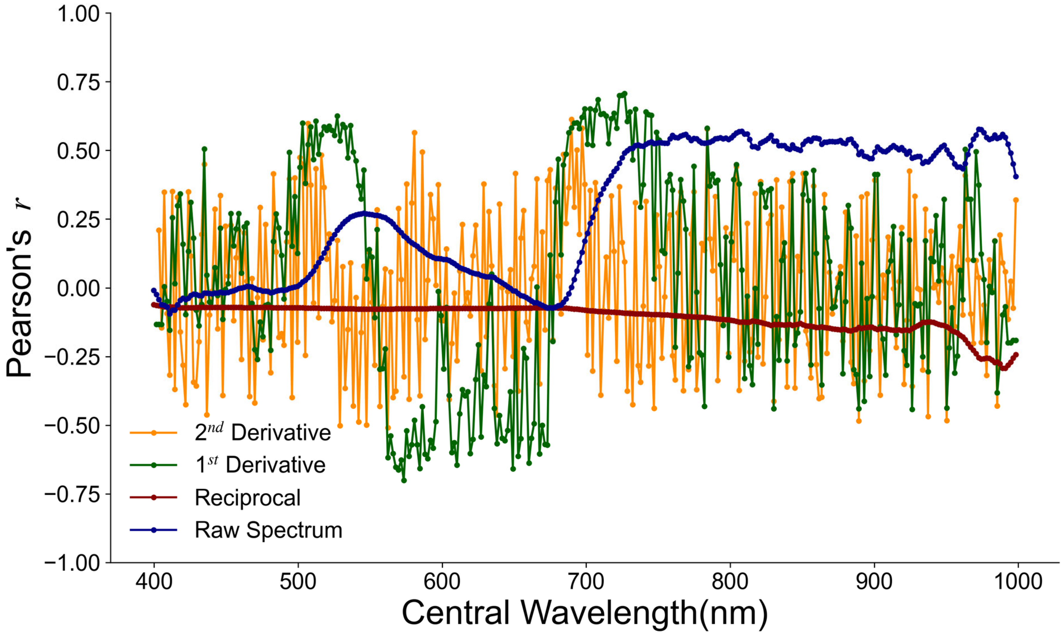
The correlation between the surface reflectance of hyperspectral bands and its transformation with LAI is shown (Figure 2). The derivatives can enhance the detection of subtle biochemical features that might be ignored by original bands. The area where the original spectral reflectance has a high correlation with LAI was concentrated in the 750 nm–1000 nm range. The spectral intervals that are sensitive to first-order and second-order derivatives of LAI mainly fall within the 520 nm–540 nm, 580 nm–650 nm, and 700 nm–750 nm ranges. Among these, there is a significant negative correlation between 580 nm–650 nm, while the other two intervals show a clear positive correlation. After the inverse transformation of the bands, the data have a lower correlation with LAI, so no bands are selected from this range. Bands with a correlation coefficient above 0.5 in the original spectra, various transformations, and vegetation indices are chosen. After removing multicollinearity using variance inflation factor analysis, the selected characteristic bands were used for model training (Table 3).
The Pearson correlation between filtered bands, vegetation indices, and LAI (Figure 3) revealed that filtered bands have good correlations with both vegetation indices and LAI, with correlation coefficients exceeding 0.55. Bands Y2 and Y3, which show a negative correlation with LAI, exhibit strong negative correlations with all other bands. Among the bands and their transformations, those with better correlations to LAI are Y1 and Y2, both with absolute values of P e a r s o n s   r of above 0.7. In the vegetation indices, the best correlations are SAVI, TVI, and SPVI, all with correlations above 0.65.

3.2. Model Performance and Validation Between Current LAI Products

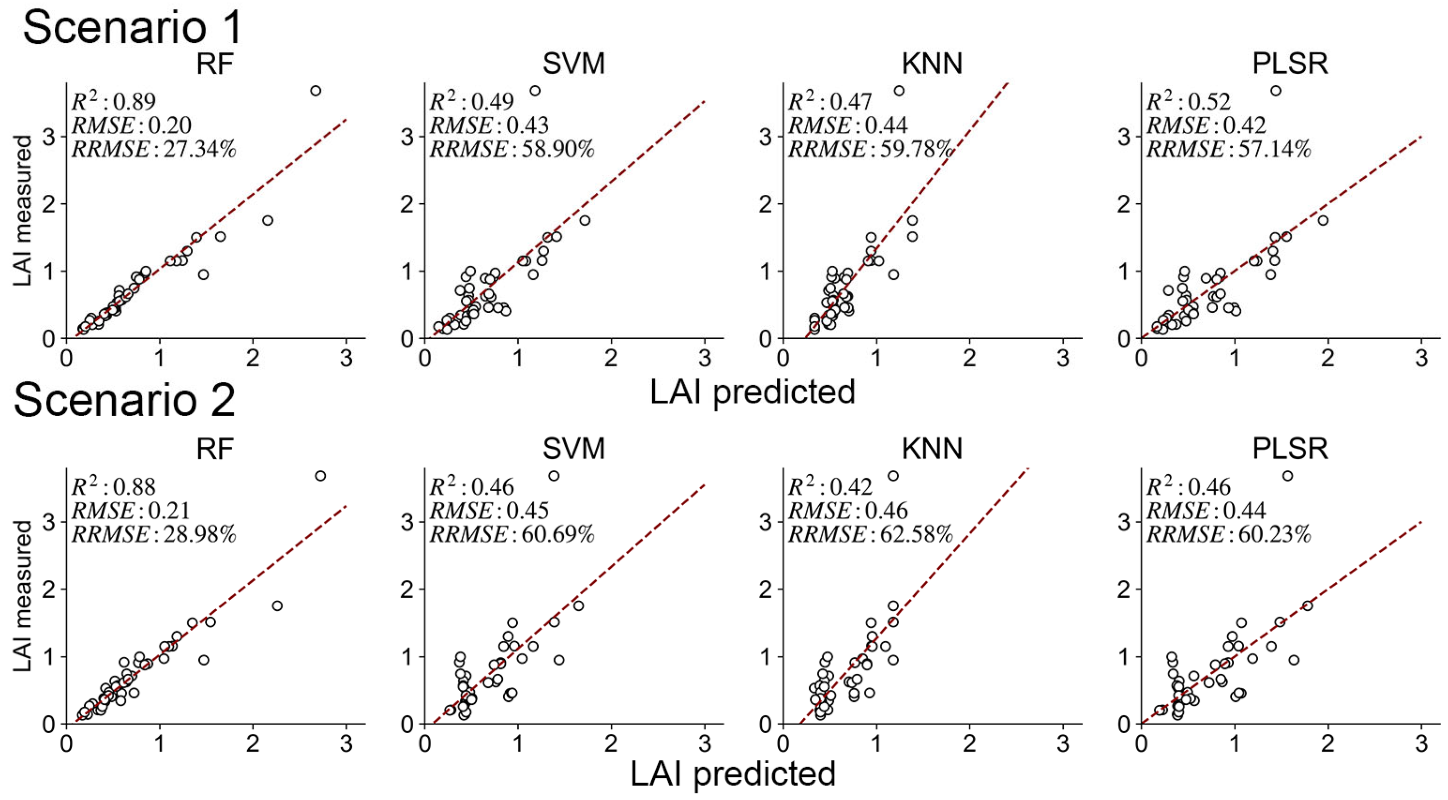
Random forest (RF), support vector machine (SVM), K-nearest neighbor (KNN), and partial least squares regression (PLSR) techniques were used to model two scenarios, one based on original spectra and transformations (Scenario 1), and the other based on hyperspectral vegetation indices (Scenario 2), the results were shown in Figure 4. Random forest (RF) consistently and significantly outperformed other models across both scenarios (testing R2 = 0.88–0.89, RMSE = 0.20–0.21, RRMSE ≈ 27–29%), with a slightly better R2, RMSE, and RRMSE in Scenario 1. SVM, KNN, and PLSR exhibited comparable performance with R2, RMSE, and RRMSE values ranging from 0.42 to 0.52, 0.42 to 0.46, and 57% to 63%, respectively. These three models all performed marginally better in Scenario 1 than in Scenario 2.
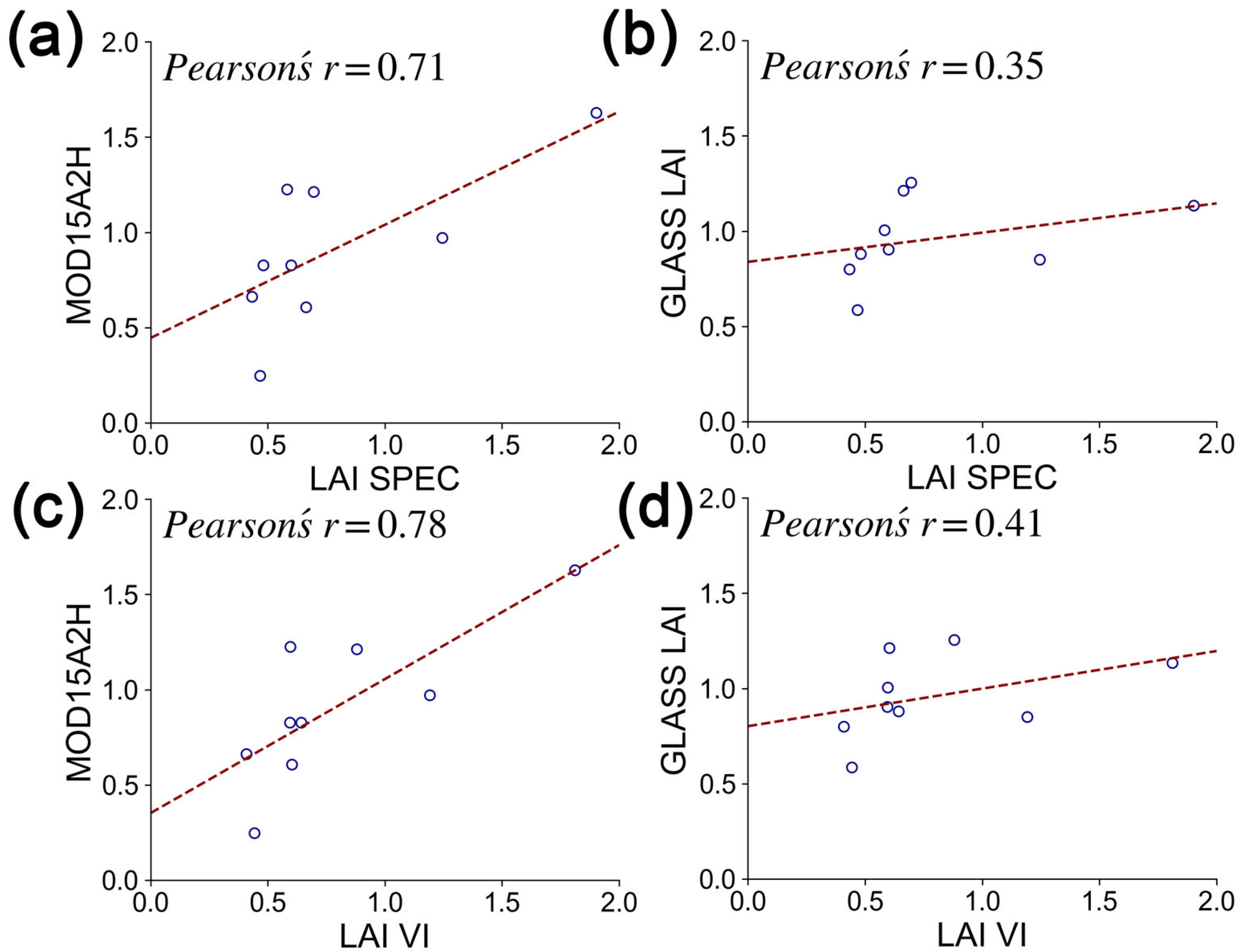
A validation was made to address the relationship between the LAI predicted in this study and a widely recognized LAI product (Figure 5). The average LAI of the whole plot (~100 m × 100 m) was generated using RF models in both scenarios to spatially match two LAI products, namely MODIS LAI (MOD15A2H) and GLASS LAI. LAI-VI consistently performed better than LAI-SPEC in correlating with both products, achieving Pearson’s r values of 0.78 (vs. MOD15A2H, Figure 5c) and 0.41 (vs. GLASS, Figure 5d), compared to LAI-SPEC’s Pearson’s r values of 0.71 (MOD15A2H, Figure 5a) and 0.35 (GLASS, Figure 5b). Moreover, both models exhibited stronger correlations with MOD15A2H than with GLASS LAI, underscoring MOD15A2H’s superior alignment with our predictions.

3.3. Uncertainty and Mapping of LAI Estimation Model Predictions

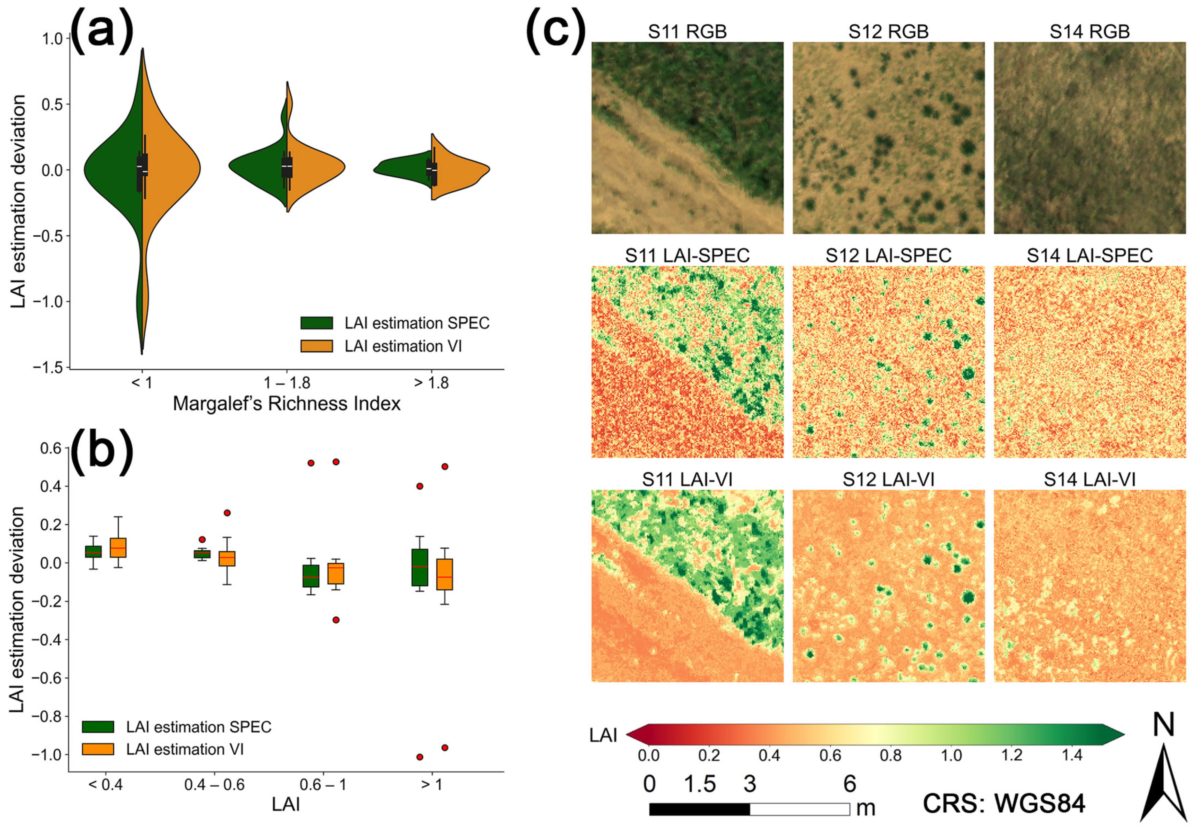
The uncertainty values (derived as the absolute value of the deviation between predicted LAI and measured LAI) of random forest models in both scenarios are shown in Figure 6, using LAI value and species richness at the quadrat level (represented by Margalef’s richness index, MRI) as classification criteria, and the interval was set unevenly to ensure that each interval had a similar amount of samples. The violin plot in Figure 6a shows that when the MRI increases, the variation of LAI estimation uncertainty of both methods decreases. The spectral data-based model (Scenario 1) showed lower uncertainty when the MRI was <1 and 1–1.8 than the VI-based model (Scenario 2), but higher uncertainty in the >1.8 interval. The box plot in Figure 6b shows the distribution of uncertainty with the measured LAI. In both models, the low uncertainty was observed when the measured LAI was low (<0.4 and 0.4–0.6); when measured LAI increases (0.6–1 and >1), the distribution of uncertainty samples tends to vary.
The predictions using RF models constructed using spectrum (LAI-SPEC) and VIs (LAI-VI) over non-sample area are shown in Figure 6c. The spatial mapping ability of two models were examined by comparing RGB image with two predictions. Notably, both models can accurately predict LAI under different grassland structures, especially in dense vegetation area. An overestimation of LAI value on bare soil was observed in both scenarios (the LAI value is expected to be 0), and LAI-VI showed larger overestimation than LAI-SPEC. In the S11 plot, the model provided a LAI prediction value of around 0.4 for bare soil pixels, whereas LAI-SPEC, on the other hand, provided a prediction of around 0.2 to 0.4 for bare soil pixels. The poor performance of both models on bare soil pixels may be due to a lack of bare soil samples. In this study, all quadrats were set in vegetated area, and pure bare soil quadrats were not included in sampling and training session. In the complex scenario of S14, where vegetation is sparse, LAI-SPEC better captures high-LAI pixels, showing an advantage over the VI-based model in terms of LAI mapping.
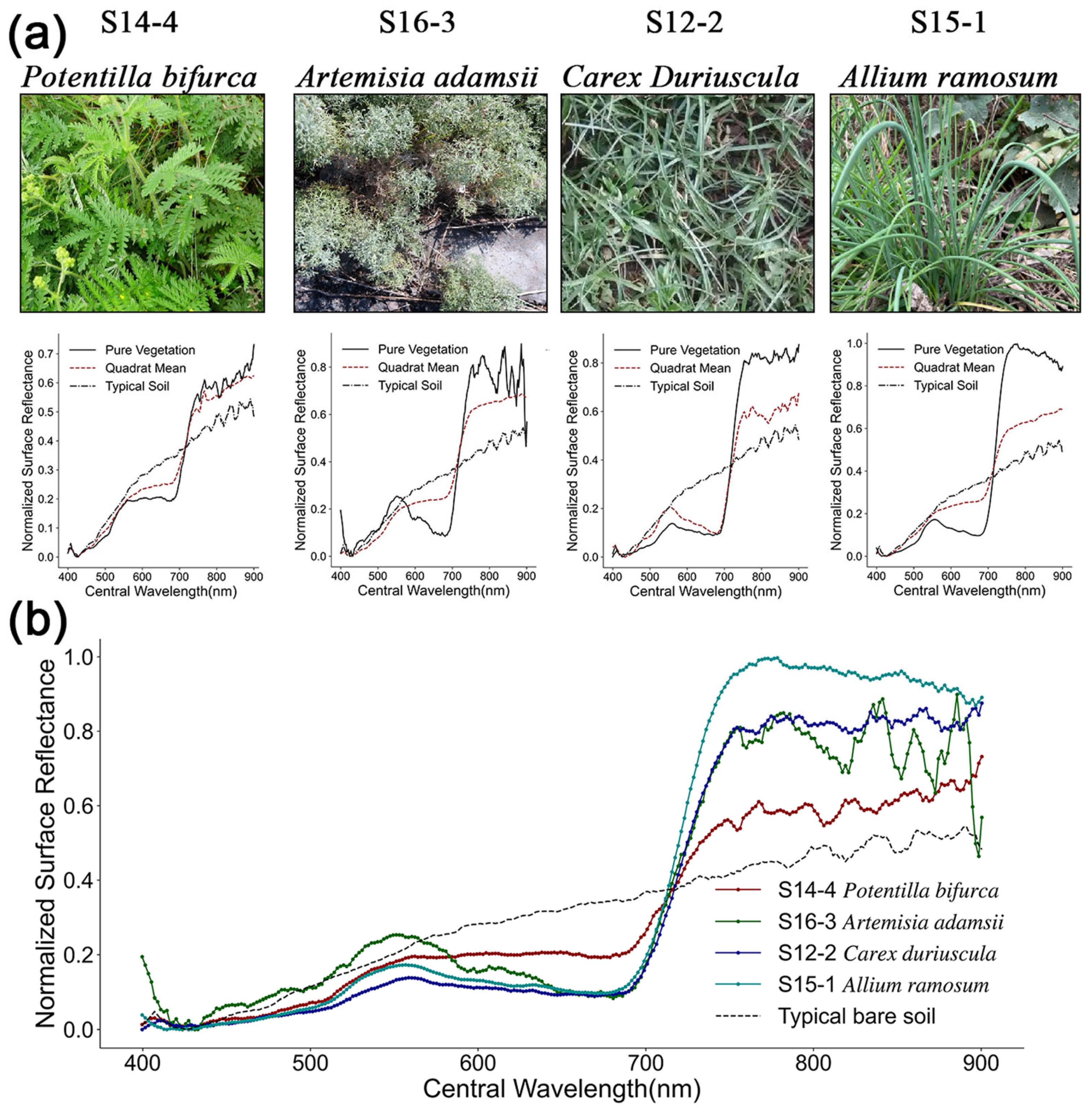
In addition to the MRI and LAI values, the uncertainty of the hyperspectral LAI inversion results is also influenced by various factors, such as dominant species and species diversity within the quadrat, and the overall canopy cover. The main dominant species in this study included Carex duriuscula, Allium ramosum, Potentilla bifurca, and Artemisia adamsi, etc. By extracting pure single-species vegetation pixels from quadrat images, we obtained normalized spectral response curves for typical dominant species (Figure 7). The spectral responses of pure vegetation pixels show strong consistency, with surface reflectance forming local peaks around the green band (550 nm) and rapidly increasing between the near-infrared bands (700–800 nm), differing from bare soil pixels. There are differences in spectra among different vegetation types; the increase in the spectral response of Artemisia adamsii at 550 nm is significantly stronger than that of other vegetation, while the peak reflectance of Allium ramosum at 770 nm is slightly higher than that of other vegetation, and it shows a slow downward trend after reaching the peak.
A statistically significant positive correlation was observed between total canopy cover and measured LAI (Pearson’s r = 0.51, p < 0.01) (Figure 8). When the total canopy cover exceeds 70%, the quadrats’ LAI is significantly higher than those with lower canopy cover. The spectral response curves of different levels of total canopy cover show significant differences between 600–700 nm; quadrats with high total canopy cover exhibit a downward trend in this range, while quadrats with total canopy cover below 50% tend to be stable. Quadrats with low total canopy cover are more influenced by bare soil pixels in the red-light band compared to vegetation. In the 850–900 nm range, quadrats with high total canopy cover show a “convex” distribution in their spectral curves, while quadrats with low total canopy cover show a “concave” shape.

3.4. Analysis of the Eigenvalue Contribution of SHAP

The SHAP analysis of the RF models in the two scenarios found that in the spectral model (Scenario 1), the contribution of each feature value to the output LAI was ranked as follows (Figure 9, detailed SHAP values of all features were listed in Table S3): Y2 (first derivative, 573.3 nm) > Z2 (second derivative, 506.8 nm) > Y1 (first derivative, 726.7 nm) > Y3 (first derivative, 649.1 nm). Among these, Y2 had a stronger explanatory power than other bands and transformations. In the VI model (Scenario 2), the contribution of the vegetation index to the model output was as follows: PPR > NDVI > TVI > SPVI. When the model output LAI is extremely high (LAI > 1.5), PPR, TVI, and SPVI all exhibit strong positive effects on the model output. When the output LAI is low, PPR and NDVI show strong negative effects.
The high explanatory power of Y2 (first derivative, 573.3 nm) likely stems from its sensitivity to subtle variations in chlorophyll absorption dynamics at the transition zone between green reflectance and red absorption, where the first derivative enhances spectral contrast related to leaf biochemical properties and canopy structure. In contrast, other features primarily capture structural or red-edge features, which may exhibit less direct coupling with LAI under varying environmental conditions, explaining Y2's superior predictive dominance. On the other hand, in the model constructed using vegetation indices (Scenario 2), several vegetation indices exhibited considerable model explanatory power in addition to the PPR because they integrate multiple spectral bands to enhance sensitivity to vegetation biophysical properties, with their differential impacts at high and low LAI levels reflecting distinct physiological and structural responses.

4. Discussion

4.1. The Influence of Spatial Heterogeneity on Model Performance

At the quadrat level, the spectral response curve integrates various species of vegetation and soil spectral characteristics within the quadrat, potentially introducing interference in accurate LAI estimation. The discrimination of the spectral response curves between different canopy covers (Figure 8c) at 600–700 nm is due to an increase in the response curve of bare soil pixels in the red-light band, whereas vegetation pixels show the opposite effect. The proportion of these two types of pixels in the quadrat determines the overall trend of the average spectral response curve. Quadrat-level species composition and total canopy cover introduce spectral variability that can bias quadrat-scale LAI inversion results, but hyperspectral data provide compensatory advantages through pixel-level separation of vegetation and non-vegetation components via continuous spectra and quadrat-level canopy cover dependent spectral weighting using spectral curve attributes between certain sensitive wavelength intervals. These techniques help to solve issues raised by the spatial heterogeneity of grasslands. For instance, previous studies have discussed the relationship between hyperspectral response and species richness [48,49], vegetation cover [50,51,52], and dominant species [53,54], all of which supplied or showed good alignments with the findings of this study.

4.2. Comparison of This Study with Existing LAI Products

LAI, as a key parameter in large-scale carbon sink estimation models, is widely used in various process mechanism models, such as Biome-BGC and BEPS [55,56,57], and in light energy utilization (LUE) models, like CASA or VPM, LAI is crucial to accurately estimate the critical parameter of the photosynthetically active radiation absorption ratio ( f P A R ) [58,59]. Currently, most models’ LAI-driven data come from mature remote sensing LAI products, like MOD15A2H and GLASS LAI [60], which are mostly based on medium-to-low-resolution surface monitoring satellites serving all ecosystem types at the global scale. However, these products have not been optimized for individual ecosystems, such as grasslands. Studies have shown that MODIS LAI products overestimate by 53% in grasslands [58]. The optimal models in this study achieved RRMSE values between 27.34% and 28.98%, substantially outperforming MODIS LAI products which exhibit RRMSE > 47% in grassland validation performed by Liu et al. [11]. The RF model constructed using VIs in this study showed good correlation with MODIS LAI (Figure 5), which may indicate a greater potential in correcting global LAI products at the region scale compared to the RF model constructed using the spectrum in this study.

4.3. Potential and Limitations of Grassland UAV Hyperspectral LAI Estimation for Optimizing the Accuracy of Regional-Scale Carbon Sink Models

Global carbon sink models require continuous LAI input data, so medium-to-low-resolution satellites with shorter revisit cycles are typically used. These satellites do not carry hyperspectral sensors, making it difficult for models based on hyperspectral bands to be directly applied to multispectral satellite remote sensing fields [61]. Hyperspectral satellites, such as PRISMA and GF-5, however, have excessively long revisit cycles and cannot provide the high temporal resolution data required by carbon sink models. Currently, most mature LAI inversion algorithms are based on RTMs, establishing lookup tables between red/near-infrared surface reflectance and LAI to find the matched LAI value [62]. A study calculated VIs for winter wheat LAI inversion using Sentinel-2 and multiple ML models, concluding that the random forest is the best model, which is similar to the findings of our study [63]. From the SHAP results of this paper, the high contributed features in the RF model constructed using VIs, such as PPR, NDVI, SPVI, and TVI, do not involve hyperspectral-unique bands, which makes it possible to reproduce the RF model constructed by VIs in this study on different satellite remote sensing platforms, such as MODIS, Landsat, Sentinel-2, etc.
This study utilized hyperspectral data from UAVs to establish an inversion model of hyperspectral data and grassland LAI at the quadrat scale. UAVs have two advantages in grassland LAI inversion, namely scale-up and scale-down. First, UAVs can scale up, which to some extent simulates the spatial heterogeneity within a pixel caused by the scale effect in LAI data used in large-scale carbon sink models. The other advantage of UAVs at the quadrat scale is that they can scale down, allowing for more accurate spatiotemporal matching with direct measurements of LAI. Whether using destructive sampling or handheld leaf area meters, the area that can be measured in a single session is limited (usually meter-level), where satellite data with spatial resolution of 10–1000 m can hardly match the direct measurement scale [64]. The UAV scale, on the other hand, generally has spatial resolutions in the centimeter range, allowing for spatio-temporal alignment with direct measurements of LAI, making model inversion results more convincing compared to results from satellite remote sensing data. Due to these two advantages, UAV-borne LAI inversion models have the potential to serve as a bridge between ground measurement and large-scale satellite monitoring. The scaling up of modeling results from drone remote sensing data is a significant direction for future research.
To reach the goal of regional refinement of LAI inputs for carbon sink models, future efforts should be focused on reproducing the LAI inversion models mentioned in this study with satellite sensors, such as Sentinel-2 and MODIS. The VI-based RF model is a better choice because the SHAP results (Figure 7) show that important features have little dependency on hyperspectral-unique VIs, which makes it possible to reproduce the model on multi-spectral sensors on satellites, and the validation results in Figure 5 have already shown good correlation between the VI-based RF model and current LAI products. The future work will include quantifying the impact of band width and central wavelength discrepancies on VI calculations, establishing sensor-specific correction coefficients, and validating model robustness within the study region. Notably, the following current limitations must be addressed: UAV data’s limited temporal coverage hinders capturing seasonal dynamics; scale mismatches between UAV and satellite pixels may introduce biases in upscaling; and model performance under extreme conditions (e.g., drought or heavy grazing) remains untested, necessitating long-term, multi-context validation.

5. Conclusions

This study utilized ML models to construct a relationship model between UAV-borne hyperspectral data and grassland LAI by screening original bands, their transformations, and vegetation indices. Our results demonstrated that the random forest model performed better than other models in both scenarios (R2 = 0.88), with model uncertainty increasing with higher measured LAI and decreasing with higher quadrat species richness. The analysis of the impact of spatial heterogeneity within quadrats on model inversion accuracy through various vegetation indicators measured within the quadrats was conducted. The LAI model constructed from UAV hyperspectral data for grasslands has great potential as an input for regional LAI data in large-scale carbon sink models. The UAV platform’s principal advantage resides in its capacity for bidirectional scaling, effectively bridging microscale ground observations and macroscale satellite applications. Additionally, the spatial heterogeneity within quadrats helps to simulate the coarse resolution issues caused by mixed pixels in ground observation satellite data to some extent. This study demonstrated the modeling accuracy and inclusiveness of spatial consistency within plots using a UAV hyperspectral data-based LAI inversion model for grasslands, laying the foundation for future research in large-scale carbon sink models.

Supplementary Materials

The following supporting information can be downloaded at: https://www.mdpi.com/article/10.3390/rs17162914/s1, Table S1: Parameters of Nano-Hyperspec hyperspectral sensor; Table S2: Grid search hyperparameter settings and best parameters for 4 models; Table S3: SHAP values for all features in both scenarios.

Author Contributions

Conceptualization, S.B., Y.F. and N.S.; data curation, Y.T., L.L., W.L., M.X., B.C. and Q.L.; formal analysis, D.W. and S.B.; funding acquisition, Q.Z. and N.S.; investigation, Y.T., L.L., S.L., M.X., B.C., Q.L. and M.C.; methodology, D.W. and Y.F.; project administration, S.L. and N.S.; Software, D.W. and S.B.; Supervision, N.S.; validation, Y.T. and W.L.; visualization, D.W.; writing—original draft, D.W. and S.B.; writing—review & editing, Y.F. and N.S. All authors have read and agreed to the published version of the manuscript.

Funding

This research was jointly funded by the First Phase of the Project of Strengthening the Scientific and Technological Research Capacity of Hulun Lake Natrue Reserve (HSZCS-C-F-210094), the Ecological Security Investigation and Assessment Project of Hulun Lake (HSZCS-G-F-210059), the National Science Foundation of China (42071050), the Taishan Scholar Project (TSQN202306210), and the Natural Science Foundation of Inner Mongolia Autonomous Region (2024ZD13).

Data Availability Statement

The original contributions presented in this study are included in the article. Further inquiries can be directed to the corresponding author.

Conflicts of Interest

The authors declare that they have no known competing financial interests or personal relationships that could have appeared to influence the work reported in this paper.

References

  1. Lal, R. Carbon Cycling in Global Drylands. Curr. Clim. Chang. Rep. 2019, 5, 221–232. [Google Scholar] [CrossRef]
  2. Bardgett, R.D.; Bullock, J.M.; Lavorel, S.; Manning, P.; Schaffner, U.; Ostle, N.; Chomel, M.; Durigan, G.; Fry, E.L.; Johnson, D.; et al. Combatting global grassland degradation. Nat. Rev. Earth Environ. 2021, 2, 720–735. [Google Scholar] [CrossRef]
  3. Chen, J.M.; Cihlar, J. Retrieving leaf area index of boreal conifer forests using landsat TM images. Remote Sens. Environ. 1996, 55, 153–162. [Google Scholar] [CrossRef]
  4. Osem, Y.; O’Hara, K. An ecohydrological approach to managing dryland forests: Integration of leaf area metrics into assessment and management. Forestry 2016, 89, 338–349. [Google Scholar] [CrossRef]
  5. De Bock, A.; Belmans, B.; Vanlanduit, S.; Blom, J.; Alvarado-Alvarado, A.A.; Audenaert, A. A review on the leaf area index (LAI) in vertical greening systems. Build. Environ. 2023, 229, 109926. [Google Scholar] [CrossRef]
  6. Fang, H.L.; Baret, F.; Plummer, S.; Schaepman-Strub, G. An Overview of Global Leaf Area Index (LAI): Methods, Products, Validation, and Applications. Rev. Geophys. 2019, 57, 739–799. [Google Scholar] [CrossRef]
  7. Cho, M.A.; Ramoelo, A.; Math, R. Estimation of leaf area index (LAI) of South Africa from MODIS imagery by inversion of PROSAIL radiative transfer model. In Proceedings of the IEEE Joint International Geoscience and Remote Sensing Symposium (IGARSS)/35th Canadian Symposium on Remote Sensing, Quebec City, QC, Canada, 13–18 July 2014; pp. 2590–2593. [Google Scholar]
  8. López-Lozano, R.; Casterad, M.A. LAI estimation by scaling up and inversion of radiative transfer models from Quickbird images. Rev. De Teledetec. 2005, 24, 43–47. [Google Scholar]
  9. Fang, H.L.; Wang, Y.; Zhang, Y.H.; Li, S.J. Long-Term Variation of Global GEOV2 and MODIS Leaf Area Index (LAI) and Their Uncertainties: An Insight into the Product Stabilities. J. Remote Sens. 2021, 2021, 9842830. [Google Scholar] [CrossRef]
  10. Fang, H.L.; Wei, S.S.; Jiang, C.Y.; Scipal, K. Theoretical uncertainty analysis of global MODIS, CYCLOPES, and GLOBCARBON LAI products using a triple collocation method. Remote Sens. Environ. 2012, 124, 610–621. [Google Scholar] [CrossRef]
  11. Liu, Y.B.; Xiao, J.F.; Ju, W.M.; Zhu, G.L.; Wu, X.C.; Fan, W.L.; Li, D.Q.; Zhou, Y.L. Satellite-derived LAI products exhibit large discrepancies and can lead to substantial uncertainty in simulated carbon and water fluxes. Remote Sens. Environ. 2018, 206, 174–188. [Google Scholar] [CrossRef]
  12. Tian, Y.H.; Woodcock, C.E.; Wang, Y.J.; Privette, J.L.; Shabanov, N.V.; Zhou, L.M.; Zhang, Y.; Buermann, W.; Dong, J.R.; Veikkanen, B.; et al. Multiscale analysis and validation of the MODIS LAI product: I. Uncertainty assessment. Remote Sens. Environ. 2002, 83, 414–430. [Google Scholar] [CrossRef]
  13. Mateen, M.; Wen, J.H.; Nasrullah; Akbar, M.A. The Role of Hyperspectral Imaging: A Literature Review. Int. J. Adv. Comput. Sci. Appl. 2018, 9, 51–62. [Google Scholar] [CrossRef]
  14. Bioucas-Dias, J.M.; Plaza, A.; Camps-Valls, G.; Scheunders, P.; Nasrabadi, N.M.; Chanussot, J. Hyperspectral Remote Sensing Data Analysis and Future Challenges. Ieee Geosci. Remote Sens. Mag. 2013, 1, 6–36. [Google Scholar] [CrossRef]
  15. Jain, N.; Ray, S.S.; Singh, J.P.; Panigrahy, S. Use of hyperspectral data to assess the effects of different nitrogen applications on a potato crop. Precis. Agric. 2007, 8, 225–239. [Google Scholar] [CrossRef]
  16. Yang, Y.C.; Nan, R.; Mi, T.X.; Song, Y.X.; Shi, F.H.; Liu, X.R.; Wang, Y.Q.; Sun, F.L.; Xi, Y.J.; Zhang, C. Rapid and Nondestructive Evaluation of Wheat Chlorophyll under Drought Stress Using Hyperspectral Imaging. Int. J. Mol. Sci. 2023, 24, 5825. [Google Scholar] [CrossRef] [PubMed]
  17. Wang, L.; Chen, S.S.; Peng, Z.P.; Huang, J.C.A.; Wang, C.Y.; Jiang, H.; Zheng, Q.; Li, D. Phenology Effects on Physically Based Estimation of Paddy Rice Canopy Traits from UAV Hyperspectral Imagery. Remote Sens. 2021, 13, 1792. [Google Scholar] [CrossRef]
  18. Toth, C.; Józków, G. Remote sensing platforms and sensors: A survey. ISPRS J. Photogramm. Remote Sens. 2016, 115, 22–36. [Google Scholar] [CrossRef]
  19. Kanning, M.; Kühling, I.; Trautz, D.; Jarmer, T. High-Resolution UAV-Based Hyperspectral Imagery for LAI and Chlorophyll Estimations from Wheat for Yield Prediction. Remote Sens. 2018, 10, 2000. [Google Scholar] [CrossRef]
  20. Yu, K.Q.; Zhao, Y.R.; Zhu, F.L.; Li, X.L.; He, Y. Mapping of Chlorophyll and SPAD Distribution in Pepper Leaves During Leaf Senescence Using Visible and Near-Infrared Hyperspectral Imaging. Trans. Asabe 2016, 59, 13–24. [Google Scholar]
  21. Bayat, B.; Van der Tol, C.; Verhoef, W. Remote Sensing of Grass Response to Drought Stress Using Spectroscopic Techniques and Canopy Reflectance Model Inversion. Remote Sens. 2016, 8, 557. [Google Scholar] [CrossRef]
  22. Ding, Z.; Zhu, X.; Ma, L.; Zhao, Y. Estimating LAI and uncertainty in grassland using UAV hyperspectral data and PROSAIL. Adv. Comput. Signals Syst. 2024, 8, 13–22. [Google Scholar] [CrossRef]
  23. Si, Y.L.; Schlerf, M.; Zurita-Milla, R.; Skidmore, A.; Wang, T.J. Mapping spatio-temporal variation of grassland quantity and quality using MERIS data and the PROSAIL model. Remote Sens. Environ. 2012, 121, 415–425. [Google Scholar] [CrossRef]
  24. Lu, B.; Proctor, C.; He, Y.H. Investigating different versions of PROSPECT and PROSAIL for estimating spectral and biophysical properties of photosynthetic and non-photosynthetic vegetation in mixed grasslands. Gisci. Remote Sens. 2021, 58, 354–371. [Google Scholar] [CrossRef]
  25. Fern, R.R.; Foxley, E.A.; Bruno, A.; Morrison, M.L. Suitability of NDVI and OSAVI as estimators of green biomass and coverage in a semi-arid rangeland. Ecol. Indic. 2018, 94, 16–21. [Google Scholar] [CrossRef]
  26. He, Y.H.; Guo, X.L.; Wilmshurst, J.F. Comparison of different methods for measuring leaf area index in a mixed grassland. Can. J. Plant Sci. 2007, 87, 803–813. [Google Scholar] [CrossRef]
  27. Imran, H.A.; Gianelle, D.; Rocchini, D.; Dalponte, M.; Martín, M.P.; Sakowska, K.; Wohlfahrt, G.; Vescovo, L. VIS-NIR, Red-Edge and NIR-Shoulder Based Normalized Vegetation Indices Response to Co-Varying Leaf and Canopy Structural Traits in Heterogeneous Grasslands. Remote Sens. 2020, 12, 2254. [Google Scholar] [CrossRef]
  28. Shen, B.B.; Ding, L.; Ma, L.C.; Li, Z.W.; Pulatov, A.; Kulenbekov, Z.; Chen, J.Q.; Mambetova, S.; Hou, L.L.; Xu, D.W.; et al. Modeling the Leaf Area Index of Inner Mongolia Grassland Based on Machine Learning Regression Algorithms Incorporating Empirical Knowledge. Remote Sens. 2022, 14, 4196. [Google Scholar] [CrossRef]
  29. Qin, G.X.; Wu, J.; Li, C.B.; Meng, Z.Y. Comparison of the hybrid of radiative transfer model and machine learning methods in leaf area index of grassland mapping. Theor. Appl. Climatol. 2024, 155, 2757–2773. [Google Scholar] [CrossRef]
  30. Tsele, P.; Ramoelo, A. Integrating Active Learning and Regression Methods for Estimation of Grass Lai Over a Mountainous Region using Sentinel-2 Satellite Data. In Proceedings of the IGARSS 2024—2024 IEEE International Geoscience and Remote Sensing Symposium, Athens, Greece, 7–12 July 2024; pp. 10516–10519. [Google Scholar]
  31. Doepper, V.; Rocha, A.D.; Berger, K.; Graenzig, T.; Verrelst, J.; Kleinschmit, B.; Foerster, M. Estimating soil moisture content under grassland with hyperspectral data using radiative transfer modelling and machine learning. Int. J. Appl. Earth Obs. Geoinf. 2022, 110, 102817. [Google Scholar] [CrossRef]
  32. Liu, Z.W.; Jiang, J.B.; Du, Y.; Xu, Z.F. A Band Influence Algorithm for Hyperspectral Band Selection to Classify Moldy Peanuts. IEEE Access 2021, 9, 147527–147536. [Google Scholar] [CrossRef]
  33. Li, J.H.; Li, Q.Z.; Wang, F.; Liu, F. Hyperspectral redundancy detection and modeling with local Hurst exponent. Phys. A-Stat. Mech. Its Appl. 2022, 592, 126830. [Google Scholar] [CrossRef]
  34. Zhang, H.; Li, X.W.; Cao, C.X.; Yang, H.; Gao, M.X.; Zheng, S.; Xu, M.; Xie, D.H.; Jia, H.C.; Ji, W.; et al. Scale effects of leaf area index inversion based on environmental and disaster monitoring satellite data. Sci. China-Earth Sci. 2010, 53, 92–98. [Google Scholar] [CrossRef]
  35. Fan, W.J.; Gai, Y.Y.; Xu, X.R.; Yan, B.Y. The spatial scaling effect of the discrete-canopy effective leaf area index retrieved by remote sensing. Sci. China-Earth Sci. 2013, 56, 1548–1554. [Google Scholar] [CrossRef]
  36. Darvishzadeh, R.; Skidmore, A.; Schlerf, M.; Atzberger, C. Inversion of a radiative transfer model for estimating vegetation LAI and chlorophyll in a heterogeneous grassland. Remote Sens. Environ. 2008, 112, 2592–2604. [Google Scholar] [CrossRef]
  37. Zhang, M.Y.; Gong, M.G.; Chan, Y.Q. Hyperspectral band selection based on multi-objective optimization with high information and low redundancy. Appl. Soft Comput. 2018, 70, 604–621. [Google Scholar] [CrossRef]
  38. Yang, C.B.; Feng, M.C.; Song, L.F.; Jing, B.H.; Xie, Y.K.; Wang, C.; Yang, W.D.; Xiao, L.J.; Zhang, M.J.; Song, X.Y. Study on hyperspectral monitoring model of soil total nitrogen content based on fractional-order derivative. Comput. Electron. Agric. 2022, 201, 107307. [Google Scholar] [CrossRef]
  39. Ceccato, P.; Flasse, S.; Tarantola, S.; Jacquemoud, S.; Grégoire, J.M. Detecting vegetation leaf water content using reflectance in the optical domain. Remote Sens. Environ. 2001, 77, 22–33. [Google Scholar] [CrossRef]
  40. Lin, Y.H.; Shen, H.F.; Tian, Q.J.; Gu, X.F.; Yang, R.R.; Qiao, B.J. Mechanisms underlying diurnal variations in the canopy spectral reflectance of winter wheat in the jointing stage. Curr. Sci. 2020, 118, 1401–1406. [Google Scholar] [CrossRef]
  41. Shebl, A.; Abriha, D.; Fahil, A.S.; El-Dokouny, H.A.; Elrasheed, A.A.; Csámer, A. PRISMA hyperspectral data for lithological mapping in the Egyptian Eastern Desert: Evaluating the support vector machine, random forest, and XG boost machine learning algorithms. Ore Geol. Rev. 2023, 161, 105652. [Google Scholar] [CrossRef]
  42. Rodríguez-Pérez, R.; Bajorath, J. Evolution of Support Vector Machine and Regression Modeling in Chemoinformatics and Drug Discovery. J. Comput. Aided Mol. Des. 2022, 36, 355–362. [Google Scholar] [CrossRef]
  43. Sumayli, M. Development of advanced machine learning models for optimization of methyl ester biofuel production from papaya oil: Gaussian process regression (GPR), multilayer perceptron (MLP), and K-nearest neighbor (KNN) regression models. Arab. J. Chem. 2023, 16, 104833. [Google Scholar] [CrossRef]
  44. Burnett, A.C.; Anderson, J.; Davidson, K.J.; Ely, K.S.; Lamour, J.; Li, Q.Y.; Morrison, B.D.; Yang, D.D.; Rogers, A.; Serbin, S.P. A best-practice guide to predicting plant traits from leaf-level hyperspectral data using partial least squares regression. J. Exp. Bot. 2021, 72, 6175–6189. [Google Scholar] [CrossRef] [PubMed]
  45. Xiong, Z.; Cui, Y.X.; Liu, Z.H.; Zhao, Y.; Hu, M.; Hu, J.J. Evaluating explorative prediction power of machine learning algorithms for materials discovery using k-fold forward cross-validation. Comput. Mater. Sci. 2020, 171, 109203. [Google Scholar] [CrossRef]
  46. Qureshi, H.; Anwar, T.; Mohibullah, M.; Fatima, S.; Younas, R.; Habiba, U.; Malik, L.; Hanif, A.; Iqbal, M. Paired plot experiments to assess impact of invasive species on native floral diversity in Pakistan. Front. Environ. Sci. 2023, 10, 1037319. [Google Scholar] [CrossRef]
  47. Zhang, J.Y.; Ma, X.L.; Zhang, J.L.; Sun, D.L.; Zhou, X.Z.; Mi, C.L.; Wen, H.J. Insights into geospatial heterogeneity of landslide susceptibility based on the SHAP-XGBoost model. J. Environ. Manag. 2023, 332, 117357. [Google Scholar] [CrossRef]
  48. Psomas, A.; Kneubühler, M.; Huber, S.; Itten, K.; Zimmermann, N.E. Hyperspectral remote sensing for estimating aboveground biomass and for exploring species richness pat-terns of grassland habitats. Int. J. Remote Sens. 2011, 32, 9007–9031. [Google Scholar] [CrossRef]
  49. Gholizadeh, H.; Gamon, J.A.; Townsend, P.A.; Zygielbaum, A.I.; Helzer, C.J.; Hmimina, G.Y.; Yu, R.; Moore, R.M.; Schweiger, A.K.; Cavender-Bares, J. Detecting prairie biodiversity with airborne remote sensing. Remote Sens. Environ. 2019, 221, 38–49. [Google Scholar] [CrossRef]
  50. Zhang, F.; Wang, C.; Pan, K.; Guo, Z.; Liu, J.; Xu, A.; Ma, H.; Pan, X. The Simultaneous Prediction of Soil Properties and Vegetation Coverage from Vis-NIR Hyperspectral Data with a One-Dimensional Convolutional Neural Network: A Laboratory Simulation Study. Remote Sens. 2022, 14, 397. [Google Scholar] [CrossRef]
  51. Pervin, R.; Robeson, S.M.; MacBean, N. Fusion of airborne hyperspectral and LiDAR canopy-height data for estimating fractional cover of tall woody plants, herbaceous vegetation, and other soil cover types in a semi-arid savanna ecosystem. Int. J. Remote Sens. 2022, 43, 3890–3926. [Google Scholar] [CrossRef]
  52. Pu, Y.; Wilmshurst, F.J.; Guo, X. Separating Shrub Cover From Green Vegetation in Grasslands Using Hyperspectral Vegetation Indices. Can. J. Remote Sens. 2024, 50, 2347630. [Google Scholar] [CrossRef]
  53. Liu, W.; Han, W.; Jin, G.; Gong, K.; Ma, J. Classification of major species in the sericite–Artemisia desert grassland using hyperspectral images and spectral feature identification. PeerJ 2024, 12, e17663. [Google Scholar] [CrossRef]
  54. Zhu, X.; Bi, Y.; Du, J.; Gao, X.; Zhang, T.; Pi, W.; Zhang, Y.; Wang, Y.; Zhang, H. Research on deep learning method recognition and a classification model of grassland grass species based on unmanned aerial vehicle hyperspectral remote sensing. Grassl. Sci. 2023, 69, 3–11. [Google Scholar] [CrossRef]
  55. Srinet, R.; Nandy, S.; Patel, N.R.; Padalia, H.; Watham, T.; Singh, S.K.; Chauhan, P. Simulation of forest carbon fluxes by integrating remote sensing data into biome-BGC model. Ecol. Model. 2023, 475, 110185. [Google Scholar] [CrossRef]
  56. Zhang, S.; Zhang, J.H.; Bai, Y.; Koju, U.A.; Igbawua, T.; Chang, Q.; Zhang, D.; Yao, F.M. Evaluation and improvement of the daily boreal ecosystem productivity simulator in simulating gross primary productivity at 41 flux sites across Europe. Ecol. Model. 2018, 368, 205–232. [Google Scholar] [CrossRef]
  57. Amiro, B.D.; Chen, J.M.; Liu, J. Net primary productivity following forest fire for Canadian ecoregions. Can. J. For. Res. 2000, 30, 939–947. [Google Scholar] [CrossRef]
  58. Fu, G.; Wu, J.S. Validation of MODIS collection 6 FPAR/LAI in the alpine grassland of the Northern Tibetan Plateau. Remote Sens. Lett. 2017, 8, 831–838. [Google Scholar] [CrossRef]
  59. Yan, K.; Park, T.; Chen, C.; Xu, B.D.; Song, W.J.; Yang, B.; Zeng, Y.L.; Liu, Z.; Yan, G.J.; Knyazikhin, Y.; et al. Generating Global Products of LAI and FPAR From SNPP-VIIRS Data: Theoretical Background and Implementation. IEEE Trans. Geosci. Remote Sens. 2018, 56, 2119–2137. [Google Scholar] [CrossRef]
  60. Ma, H.; Liang, S.L. Development of the GLASS 250-m leaf area index product (version 6) from MODIS data using the bidirectional LSTM deep learning model. Remote Sens. Environ. 2022, 273, 112985. [Google Scholar] [CrossRef]
  61. Sara, D.; Mandava, A.K.; Kumar, A.; Duela, S.; Jude, A. Hyperspectral and multispectral image fusion techniques for high resolution applications: A review. Earth Sci. Inform. 2021, 14, 1685–1705. [Google Scholar] [CrossRef]
  62. Cheng, J.P.; Yang, H.; Qi, J.B.; Sun, Z.D.; Han, S.Y.; Feng, H.K.; Jiang, J.Y.; Xu, W.M.; Li, Z.H.; Yang, G.J.; et al. Estimating canopy-scale chlorophyll content in apple orchards using a 3D radiative transfer model and UAV multispectral imagery. Comput. Electron. Agric. 2022, 202, 107401. [Google Scholar] [CrossRef]
  63. Mudi, S.; Paramanik, S.; Behera, M.D.; Prakash, A.J.; Deep, N.R.; Kale, M.P.; Kumar, S.; Sharma, N.; Pradhan, P.; Chavan, M.; et al. Moderate resolution LAI prediction using Sentinel-2 satellite data and indirect field measurements in Sikkim Himalaya. Environ. Monit. Assess. 2022, 194, 897. [Google Scholar] [CrossRef]
  64. Tsele, P.; Ramoelo, A.; Qabaqaba, M.; Mafanya, M.; Chirima, G. Validation of LAI, chlorophyll and FVC biophysical estimates from sentinel-2 level 2 prototype processor over a heterogeneous savanna and grassland environment in South Africa. Geocarto Int. 2022, 37, 14355–14378. [Google Scholar] [CrossRef]
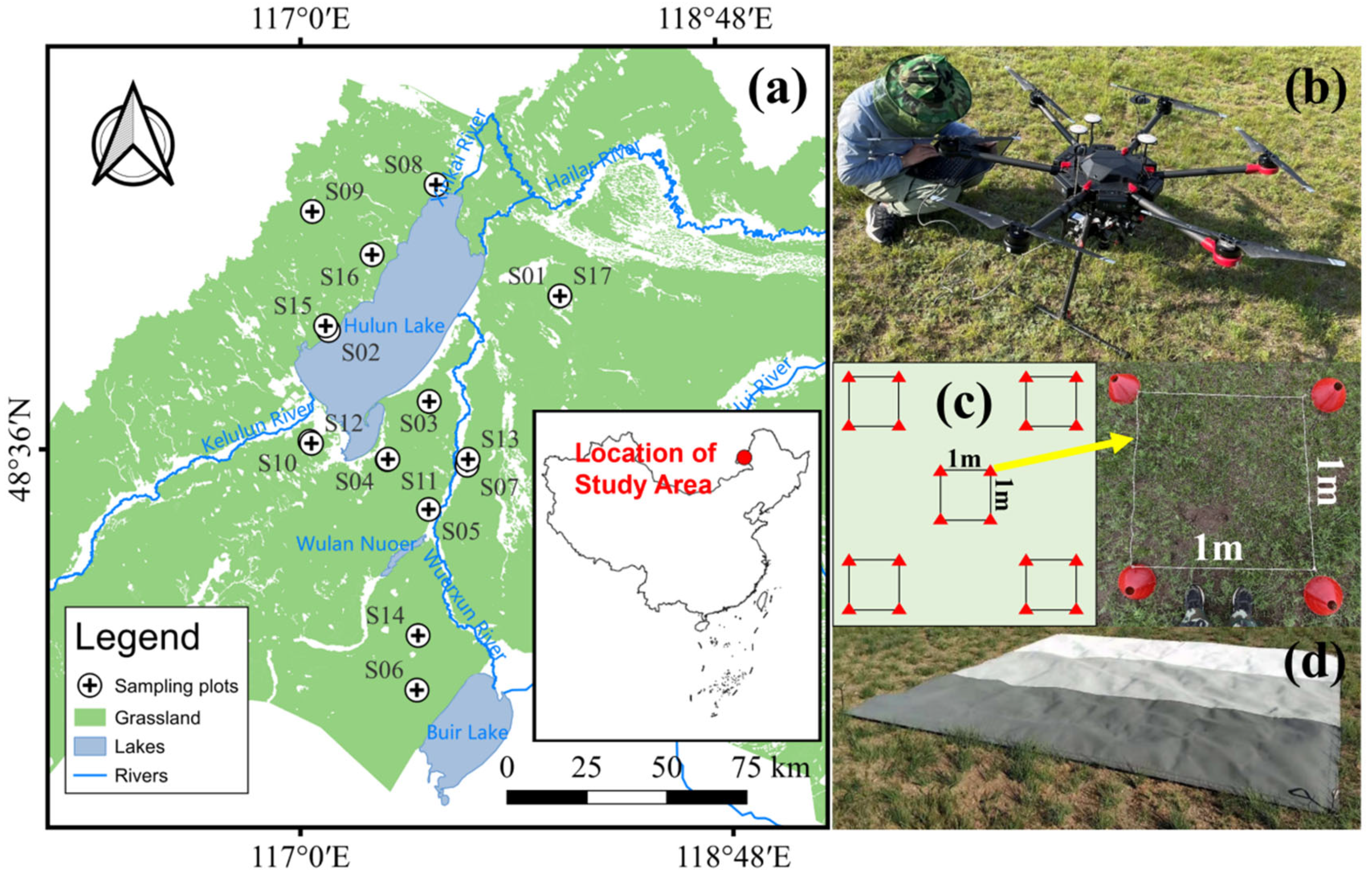
Figure 1. Location of the study area and plot setting. (a) Study area location. (b) UAV platform: DJI M600 pro. (c) Plots and quadrats setting. (d) Calibration panel.
Remotesensing 17 02914 g001
Figure 2. Pearson correlation between quadrat original reflectance and its transformation and LAI.
Remotesensing 17 02914 g002
Figure 3. Pearson correlation heat map between selected variables and LAI. The numbers represent Pearson’s r.
Remotesensing 17 02914 g003
Figure 4. Comparison of LAI modeling results between Scenario 1 (original spectra and transformations) and Scenario 2 (vegetation indices).
Remotesensing 17 02914 g004
Figure 5. Comparison between LAI prediction in this study using RF models in two scenarios (LAI SPEC and LAI LAI) and LAI products (MOD15A2H and GLASS); the LAI prediction is the average LAI in a whole plot (~100 m × 100 m) to match the spatial resolution of the LAI products.
Remotesensing 17 02914 g005
Figure 6. (a) Absolute LAI estimation deviation in different species richness samples; (b) absolute LAI estimation deviation in different measured LAI samples; (c) spatial distribution of LAI modeling results in the sample plots. From top to bottom are RGB composite image, LAI mapping visualization using the random forest model in Scenario 1, and LAI mapping visualization using the random forest model in Scenario 2.
Remotesensing 17 02914 g006
Figure 7. Quadrat level spectrum response curves. (a) Spectral response curves of typical dominant species and bare soil, and pictures of grass species; (b) spectral response curves of pure vegetation, sample average, and typical bare soil within a single dominant species quadrat.
Remotesensing 17 02914 g007
Figure 8. Relationship between quadrat canopy cover and LAI. (a,b) Relationship between quadrats’ total canopy cover and LAI; (c) spectral response curves (normalized) for different quadrat canopy cover levels; the dashed red squares represent region where the canopy cover shows differences.
Remotesensing 17 02914 g008
Figure 9. Schematic diagram of SHAP values for each feature. (a) Scenario 1; (b) Scenario 2. Black line above represents the LAI value output by the model, the black bar on the right shows the absolute size of the SHAP values for each feature, and the central heat map illustrates the SHAP values of different features under a single input.
Remotesensing 17 02914 g009
Table 1. Quality control conditions for hyperspectral data in the sample area.
Quality Control StandardsThreshold
Surface reflectance (ρ)0 < ρ < 1
Noise–signal ratio > 30
Solar zenith angle < 30 °
Light conditionsClear and cloudless
Table 2. Vegetation indices names and their abbreviations used in this study.
NameFormula NameFormula
Conventional VIsNormalized difference vegetation index (NDVI)(R800 − R670)/(R800 + R670)Hyperspectral-specific VIsNormalized difference red-edge index (NDRE)(R790 − R720)/(R790 + R720)
Soil-adjusted vegetation index (SAVI)1.5 × (R800 − R670)/(R800 + R670 + 0.5)Chlorophyll red-edge index (Clre)R750/R720 − 1
Optimized soil-adjusted vegetation index (OSAVI)1.16 × (R800 − R670)/(R800 + R670 + 0.16)Modified red-edge simple ratio index (mSR705)(R750 − R445)/(R705 − R445)
Green-normalized difference vegetation index (GNDVI)(R750 − R550)/(R750 + R550)Modified red-edge-normalized difference vegetation index (mND705)(R750 − R705)/(R750 + R705 − 2R445)
Chlorophyll green index (Clgreen)R800/R560−1Meris terrestrial chlorophyll index (MTCI)(R750 − R710)/(R710 − R680)
Plant pigment ratio (PPR)(R550 − R450)/(R550 + R450)Anthocyanin reflectance index (ARI)(1/R559)/(1/R721)
Two-band enhanced vegetation index (EVI2)2.5 × (R800 − R670)/(R800 + 2.4 × R670 + 1)Greenness index (GI)R554/R667
Red-edge normalized vegetation index (NDVI705)(R750 − R705)/(R750 + R705)Plant biochemical index (PBI)R810/R560
Triangular vegetation index (TVI)0.5 × [120(R800 − R550) − 200(R670 − R550)]Spectral polygon vegetation index (SPVI)0.4 × [3.7(R800 − R670) − 1.2(R530 − R670)]
Enhanced vegetation index (EVI)2.5(R864 − R660)/(R864 + 6R660 − 7.5R487 + 1)Transformed chlorophyll absorption in reflectance index (TCARI)3 × [(R700 − R670)− 0.2(R700 − R550)(R700/R670)]
Table 3. Results of band selection, X1–X3: original bands, Y1–Y3: first derivatives, Z1–Z3: second derivatives.
Spectrum
Variables
Central Wavelength (nm) P e a r s o n s   r Vegetation Indices P e a r s o n s   r
X1972.50.58NDVI0.55
X28080.57SAVI0.63
X3769.20.56PPR0.54
Y1726.70.71EVI20.65
Y2573.3-0.70TCARI0.62
Y3649.1-0.66TVI0.67
Z1689.30.61SPVI0.65
Z2506.80.60EVI0.59
Z3784.00.58
Disclaimer/Publisher’s Note: The statements, opinions and data contained in all publications are solely those of the individual author(s) and contributor(s) and not of MDPI and/or the editor(s). MDPI and/or the editor(s) disclaim responsibility for any injury to people or property resulting from any ideas, methods, instructions or products referred to in the content.