Article

Remote Sensing Assessment of Trophic State in Reservoir Tributary Embayments Based on Multi-Source Data Fusion

1
College of Water Conservancy and Hydropower Engineering, Hohai University, Nanjing 210098, China
2
China Yangtze Power Co., Ltd., 1 Jianshe Rd, Yichang 443002, China
*
Author to whom correspondence should be addressed.
Remote Sens. 2025, 17(16), 2886; https://doi.org/10.3390/rs17162886
Submission received: 15 July 2025 / Revised: 10 August 2025 / Accepted: 18 August 2025 / Published: 19 August 2025

Abstract

Monitoring water quality in narrow tributary bays of large river-type reservoirs is hindered by sparse sampling and cloud-limited imagery. This study develops a Trophic State Index (TSI) inversion for Xiangxi Bay, a major tributary bay of the Three Gorges Reservoir, using Landsat data and a backpropagation (BP) neural network, with hyperparameters tuned via a grid search algorithm (GSA). Environmental drivers such as water temperature, solar radiation, and photosynthetically active radiation were combined with Landsat spectral bands. Eleven sites measured monthly in 2009 yielded 98 samples after preprocessing, and training achieved R2 = 0.94. Predictions for 2009 show clear spatiotemporal heterogeneity: those for April and September (TSI = 48–59) exceeded those for July and October (46–56), with mid–lower reaches (52–59) being higher than mid–upper reaches (47–54). Out-of-period predictions for April/June 2019 and August/November 2020 were consistent with seasonal expectations, with higher spring–summer TSIs (2019: 50–57; 2020 August: 45–55) than in November 2020 (37–47). Key limitations include the small sample size, cloud-related data gaps, and sensitivity to evolving reservoir operations. This framework demonstrates a practical route to the satellite-based monitoring and mapping of trophic status in narrow reservoir tributaries.

1. Introduction

Safeguarding water quality is a core concern in aquatic environment protection, and it is directly linked to ecosystem health and the sustainable development of human society [1]. In recent decades, rapid economic expansion and intensified anthropogenic activities have exacerbated water pollution [2]. Discharges from industrial and agricultural sources, together with nitrogen- and phosphorus-laden runoff, have accelerated eutrophication [3], threatening aquatic ecosystem functions. Eutrophication also undermines fisheries and residents’ quality of life, while increasing the complexity and cost of water resource management [4]. The Trophic State Index (TSI), as a key metric for assessing eutrophication, provides an integrated evaluation of water quality. Accordingly, the efficient monitoring and accurate prediction of the TSI have become critical challenges in the field of water environmental protection, which is essential for the timely mitigation of eutrophication.
As one of the world’s largest hydraulic engineering projects, the Three Gorges Reservoir profoundly affects the surrounding aquatic environment, with particularly pronounced impacts on narrow, channel-type tributary bays such as Xiangxi Bay [5]. Reservoir impoundment and regulation markedly reduce flow velocity and discharge within these bays, prolonging the water residence time and promoting nutrient accumulation [6]. These changes, in turn, increase the risk of eutrophication and algal blooms [7]. Nutrient concentrations in such bays are modulated by temperature, wind speed, precipitation, and pollutant loads, exhibiting strong spatiotemporal heterogeneity [8,9]. Long-term, efficient water quality monitoring is therefore essential for timely problem diagnosis, the assessment of reservoir operation outcomes, and guidance on ecological restoration.
Accurate monitoring and assessment of trophic status are pivotal to sustainable water resource management and environmental protection [10,11]. Most remote sensing analyses of the TSI have focused on large, open water bodies, while studies of narrow, river-like tributary zones in reservoirs remain limited [12]. Additionally, water quality data in these areas are scarce due to constraints in the spatial distribution of monitoring sites. Consequently, available water quality data in these areas are often insufficient, posing challenges to achieving comprehensive, continuous watershed-scale monitoring. Traditional monitoring is constrained by high sampling costs, low spatiotemporal resolution, and incomplete spatial coverage [13]. These limitations are particularly pronounced in narrow water bodies such as Xiangxi Bay, where traditional approaches provide only localized point measurements, failing to capture watershed-scale water quality patterns [14]. As a result, spatial data gaps remain substantial, and available data sources are relatively scarce. Satellite-based water quality inversion and forecasting thus constitute critical means of enhancing dynamic monitoring capabilities [15]. Recently, frameworks combining remote sensing with machine learning have advanced significantly [10,16], leveraging the spatiotemporal continuity of satellite observations with the self-learning capacity of artificial intelligence to improve monitoring accuracy and efficiency [17].
Most current investigations couple remote sensing data with machine learning models for water quality inversion and prediction, yet variable selection and model parameter optimization remain limiting factors [18]. For example, He et al. estimated five individual water quality variables using a back-propagation (BP) neural network model [19], while Cao et al. highlighted ongoing challenges in inland water remote sensing and retrieved eight separate parameters [20]. These studies, centered on single indicators, cannot fully characterize the overall trophic state of water bodies. By contrast, the present study consolidates multiple water quality parameters into a single TSI, enabling concise yet comprehensive evaluation and enhancing the practical value of remote sensing inversion. Wang et al. showed that optimizing neural network parameters significantly reduces the risk of convergence to local minima and improves prediction stability [21]. Guo et al. further enhanced inversion precision by tuning BP neural network parameters using partial least squares and particle swarm optimization [22]. Building on these insights, we employ the intuitive grid search algorithm (GSA) to refine model parameters and further boost predictive capability. Moreover, the intricate water color and hydrodynamic conditions of long, channel-type tributaries lead to large fluctuations in pigment, CDOM, and suspended sediments, producing highly variable optical properties that complicate remote sensing inversion [23]. Models relying solely on spectral information are therefore inadequate. Thus, we incorporate environmental variables—water temperature (WT), wind speed (WS), and total solar radiation (SR)—into the inversion framework.
Building upon the above background, this study focuses on Xiangxi Bay and proposes a TSI inversion model that integrates multi-source environmental data with satellite observations. The model is further optimized using a grid search algorithm to fine-tune the BP neural network parameters. The resulting model supports TSI inversion across a range of trophic conditions in long, channel-type reservoir tributary bays, and performs well in validation, offering technical support and a practical reference for water quality monitoring and evidence-based management.

2. Study Area and Data Collection

2.1. Study Area

The Three Gorges Dam is located on the upper Yangtze River (Figure 1). The impounded reach forms a long (~650 km) and narrow reservoir (500–1000 m) with a normal pool level of 175 m. Xiangxi Bay, the nearest primary tributary, lies 34.5 km up-stream. Originating in the Shennongjia region, it flows 97.3 km through Xingshan County before discharging into the Yangtze River at Guizhou Town in Zigui County. This narrow, elongated mountain stream exhibits a pronounced elevation drop between its upper and lower reaches, averaging with a gradient of ~0.27%. Its stage remains nearly synchronous with the dam’s operational level, facilitating intensive navigation. Exceptionally rich in phosphorus, Xiangxi Bay constitutes a major national phosphorus source.
During Three Gorges Reservoir impoundment and release, Xiangxi Bay and Yangtze main channel waters undergo backflow-induced mixing and vertical exchange [24]. At the Xiangxi estuary, nutrients and sediments from both the Xiangxi and Yangtze channels interact dynamically. Reservoir impoundment reduces Xiangxi flow velocity via backflow effects, promoting sediment deposition [25]. Whereas the Three Gorges Reservoir mainstream is still considered mesotrophic, episodic algal blooms have been reported to occur in the weakly flushed tributary embayments. Relevant studies have demonstrated that algal blooms in Xiangxi Bay are strongly linked to hydrodynamic and environmental conditions [26]. For example, high nutrient concentrations could increase the risk of algal blooms [27]. Understanding the dynamics of trophic state in tributary waters is therefore important for the holistic management of important reservoirs.

2.2. Data Collection

Unlike broad lakes, Xiangxi Bay is a narrow and elongated water body, restricting monitoring point placement and water quality data availability. Moreover, remote sensing satellites are susceptible to cloud cover, which obscures the water surface and degrades the quality of usable imagery and reflectance retrieval. Given that Three Gorges Reservoir impoundment began in 2003 and the project was completed in 2009, our study period was defined as February to October 2009 based on available satellite imagery and corresponding field-measured water quality data. Finally, after data preprocessing and screening, the training set comprised 98 sample points.

2.2.1. Water Quality Indicator Data

To enable a comprehensive and objective assessment of the aquatic environment and nutrient status within the study area, 11 sampling sites were established and evenly distributed across the watershed (Figure 1). The narrow, river-like shape of Xiangxi Bay and limited access along the channel constrained how far sampling points could be spread laterally. Given the small spatial extent of the tributary, the small water surface area it covers, and minimal effects from weakly eroded regions, sampling points were not included in bay areas. Monthly measurements of total phosphorus (TP), total nitrogen (TN), chlorophyll-a (Chl-a), and dissolved oxygen (DO) were collected throughout the entire study period. All sampling, monitoring, and laboratory analytical procedures were strictly conducted in accordance with the Technical Specifications for Surface Water Quality Monitoring.

2.2.2. Remote Sensing Data

Google Earth Engine (GEE) offers comprehensive remote sensing data repositories, including the Landsat series, thus revolutionizing conventional processing frameworks. Landsat 5 and 7 provide a spatial resolution of 30 m and a 16-day revisit cycle. Although Landsat 5 was decommissioned in 2012, we maintained model continuity beyond this date by retrieving seven-band surface reflectance data from both Landsat 5 and 7 on GEE for Xiangxi Bay trophic status inversion. During the study period, 17 Landsat 5 and 7 scenes were acquired from GEE. Owing to frequent cloud cover, many scenes were incomplete or missing. After quality filtering, five cloud-free, high-quality scenes covering the study area were selected for constructing the TSI inversion model.

2.2.3. Meteorological Data

For the trophic state assessment, open-access meteorological datasets corresponding to each sampling date were retrieved from NOAA’s National Centers for Environmental Information (NCEI). Water temperature (WT) (°C) and wind speed (WS) (m/s) recorded from the Yichang station were extracted and preprocessed to calculate monthly averages. Total solar radiation (SR) (W/m2) and photosynthetically active radiation (PAR) (W/m2) were obtained from the National Ecological Science Data Center.

3. Methodology

3.1. TSI Inversion Model Framework

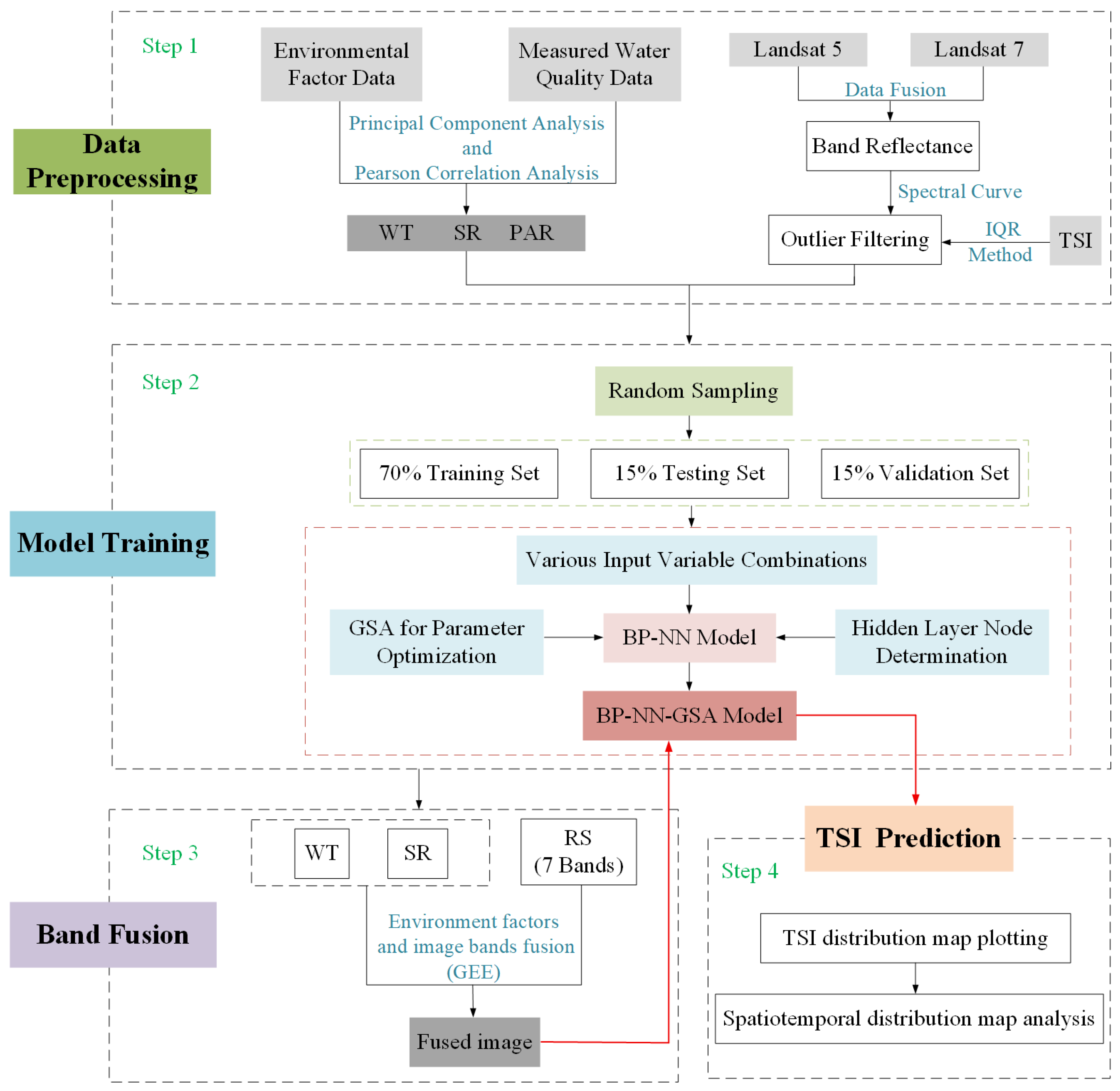
As shown in Figure 2, the framework of the TSI inversion model was based on a BP-NN-GSA method, using remote sensing and environmental data as input variables. A back-propagation neural network (BP-NN) was developed and optimized using a grid search algorithm (GSA) for the inversion of the TSI in Xiangxi Bay. The GSA was used to enhance model accuracy. After parameter tuning, the model was used to generate spatiotemporal distributions of the TSIs.
Key environmental variables were identified through Pearson correlation analysis and integrated with remote sensing reflectance (RS) bands to form multiple candidate input feature sets for model training. Model performance was evaluated across these feature sets to determine the highest-performing combination, which was subsequently integrated into GEE to produce consolidated imagery. The fused dataset was then used as input to the BP-NN to predict the final estimates of TSI distribution (Figure 2).

3.2. Data Preprocessing

3.2.1. Meteorological and Water Quality Data Preprocessing

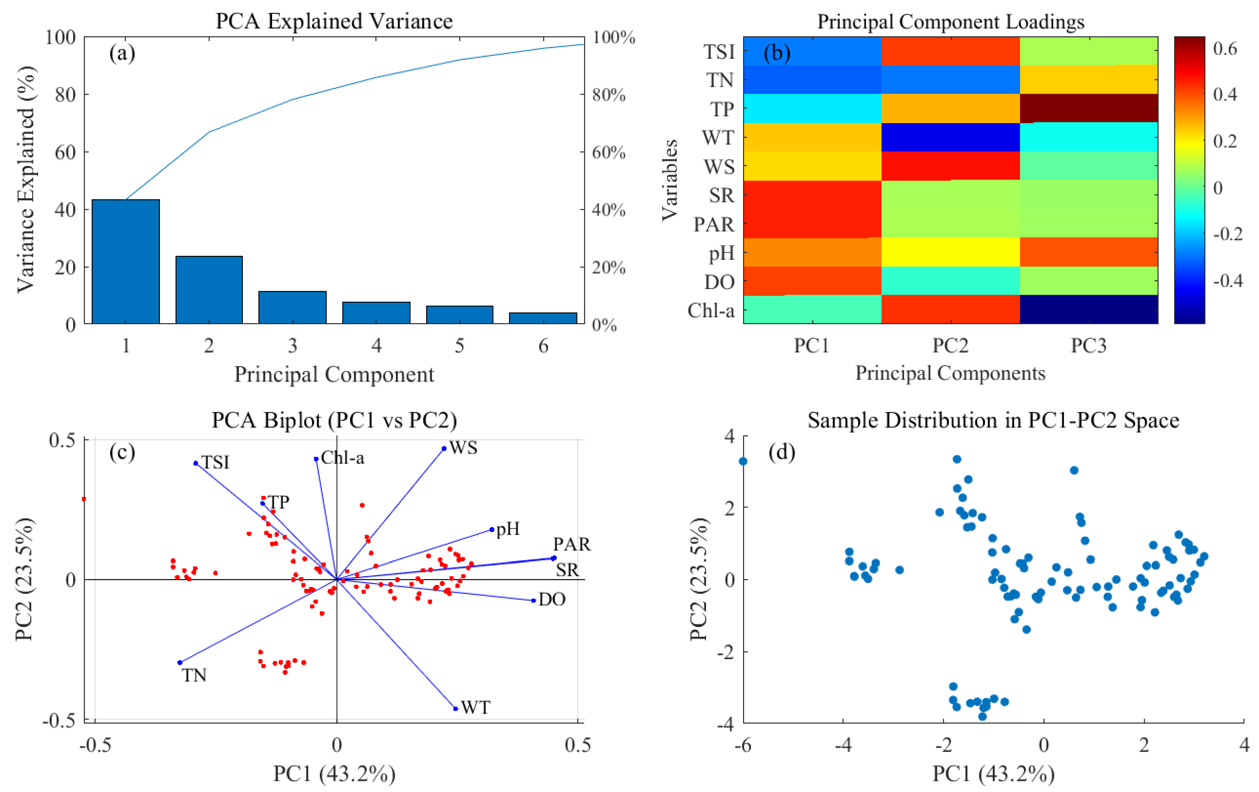
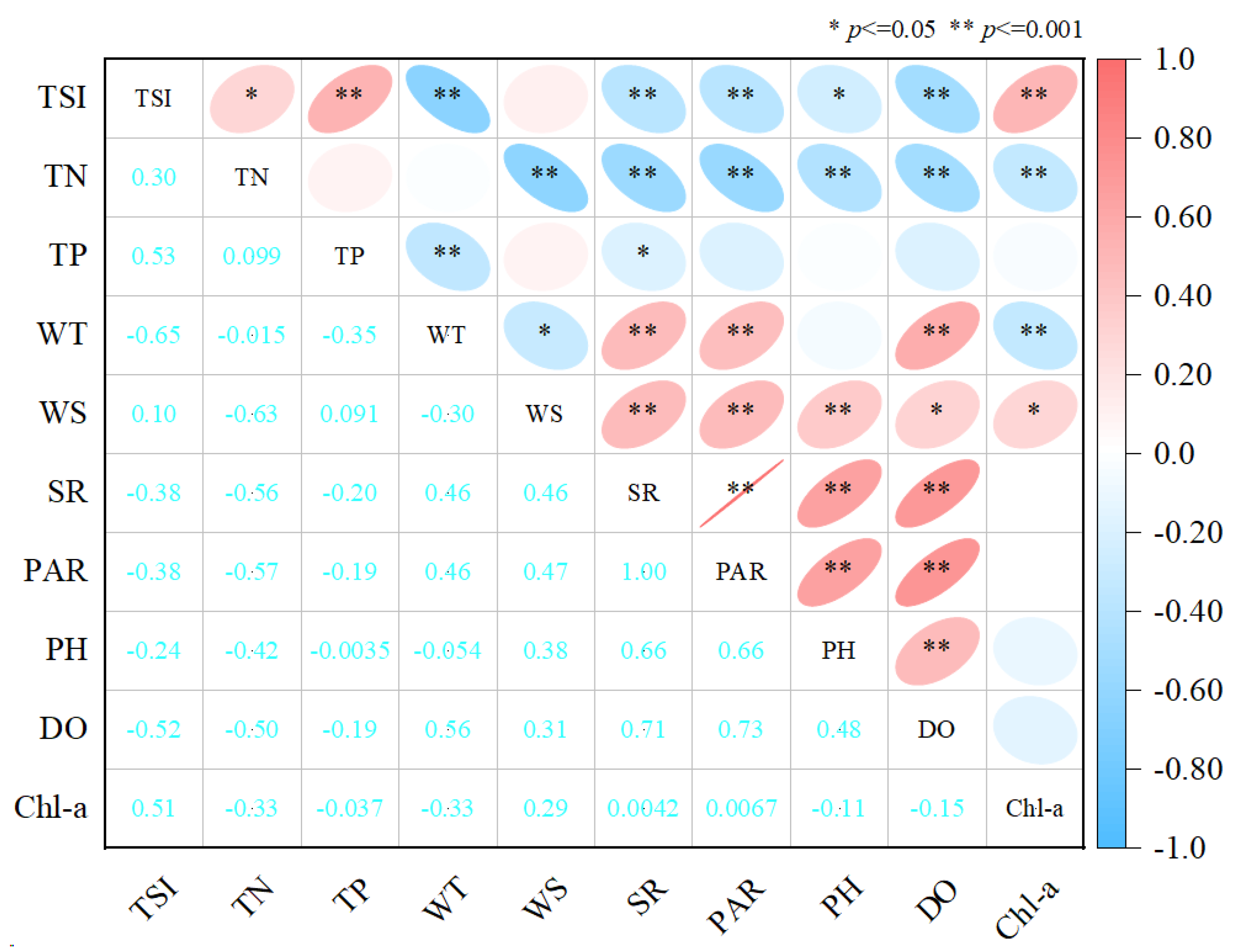
In this study, we evaluated environmental variables and water quality indicators comprehensively. Environment variables include WS, WT, SR, and PAR. Water quality indicators include TN, TP, pH, DO, and Chl-a. The optimal input variables for the inversion model were identified by measuring environmental and nutrient indicators, and then applying principal component analysis (PCA; Figure 3) and computing Pearson correlation coefficients with heat maps (Figure 4) to compare these indicators against the TSI.
PCA is an unsupervised linear dimensionality reduction technique that finds directions of maximum variance known as principal components to reduce feature count, cut complexity and noise, improve training efficiency, and alleviate multicollinearity [28]. By projecting high-dimensional data into a lower-dimensional space, PCA highlights the most informative patterns in the dataset.
Figure 3 presents the PCA results. Panel (a) shows that PC1 and PC2 explain 43.2% and 23.5% of the total variance, respectively, for a cumulative 66.7%, indicating that these two dimensions capture the most variability. In panel (b), PC1 loads heavily on SR, PAR, DO and pH, highlighting physical and light-related influences, while PC2 is dominated by TP, Chl-a and the TSI, reflecting nutrient enrichment. PC3 loads primarily on WT, revealing its distinct role. The biplot in panel (c) shows that SR and PAR aligned closely, confirming strong collinearity, and TP, Chl-a and TSI clustered along PC2. TN points in the opposite direction with regards to PC2, suggesting an antagonistic relationship. Finally, the sample distribution in the PC1–PC2 space (d) reveals distinct clusters and a few outliers, indicating that light-related gradients and nutrient factors drive site separation. Based on these patterns, SR (or PAR), Chl-a, TP, TN, WT and pH are recommended as key variables for subsequent modeling or classification, with either SR or PAR retained to avoid redundancy.
The Pearson correlation heat map was then examined. WT is strongly correlated with the TSI and key water quality parameters: Chl-a, TP, and DO (Figure 4). Previous studies have identified that high WT could induce thermal stratification, alter hydrodynamic processes, and significantly influence trophic shifts and thus is close related to algal blooms [27]. Accordingly, WT was included as an input variable in the TSI assessment model.
Although WS exhibits only a weak correlation with the TSI, it shows a strong positive correlation with Chl-a and TN. Previous studies have shown that WS modulates surface hydrodynamics, thereby altering the spatial distribution of phytoplankton at the air–water interface, and serves as a key external driver of eutrophication and algal bloom outbreaks [29]. Because WS correlations can be unstable in small datasets and risk introducing noise, WS was excluded from the input variables.
SR and PAR exhibited strong positive correlations with the TSI. Several studies have shown that PAR levels are tightly coupled with Chl-a concentration and phytoplankton growth in aquatic environments [30,31,32,33], highlighting the nexus between nutrient status and optical properties. Accordingly, SR and PAR were considered candidate input features for the inversion model. However, the extremely high inter-correlation between SR and PAR induced severe multicollinearity, which can bias model estimates. To prevent prediction distortion, it is inadvisable to include highly collinear predictors simultaneously [34].
Based on this analysis, WT, SR and PAR were selected as the environmental input variables for model training.

3.2.2. Preprocessing of the Trophic State Index (TSI)

The TSI and light absorption characteristics exhibit significant variations in their spatial and temporal distribution [35,36]. The calculation formula for the TSI value is shown in Equation (1). The TSI values can be categorized into five levels: oligotrophic (<30), mesotrophic (30 < TSI < 50), mildly eutrophic (50 < TSI <60), moderately eutrophic (60 < TSI < 70), and heavily eutrophic (>70) [23].
T S I = T S I ( C h l a ) + T S I ( T P ) + T S I ( T N ) 3
T S I ( C h l a ) = 10 ( 2.5 + 1.086 × ln C h l a )
T S I ( T P ) = 10 ( 9.436 + 1.624 × ln T P )
T S I ( T N ) = 10 ( 5.453 + 1.694 × ln T N )
Units in the equations are Chl-a (mg m−3), TP (mg L−1) and TN (mg L−1).
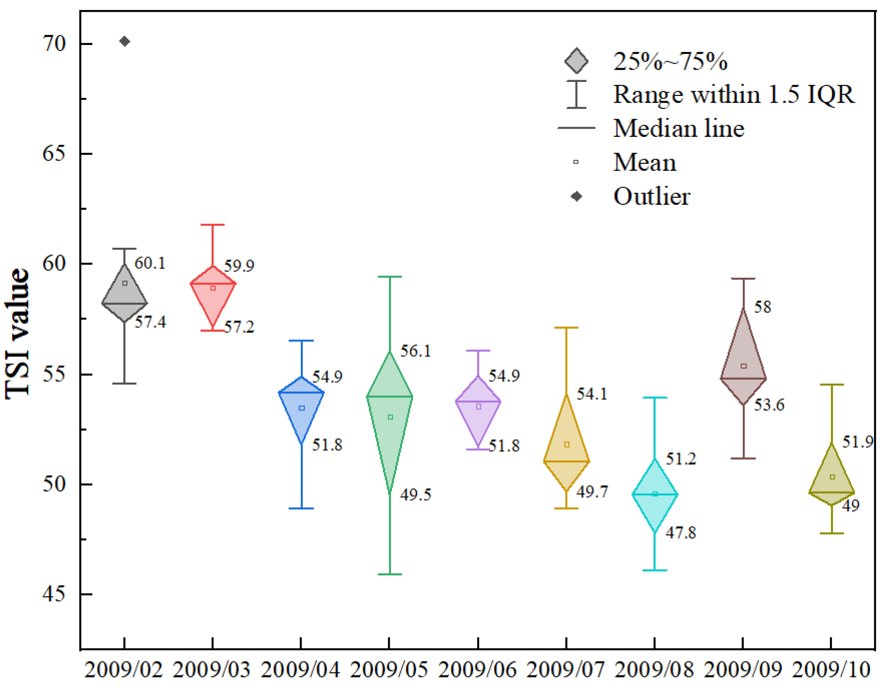
Given the potential for outliers in water quality measurements during sampling, we applied the Interquartile Range (IQR) method to detect and remove TSI outliers. The IQR is a widely used outlier detection technique that entails ordering the dataset, calculating the first quartile (Q1, 25th percentile) and third quartile (Q3, 75th percentile), and excluding values falling outside the range [Q1 – 1.5 × IQR, Q3 + 1.5 × IQR] [37].
I Q R = Q 3 Q 1
Determination of Upper and Lower Boundaries:
U p p e r = Q 3 + 1.5 × I Q R
L o w e r = Q 1 1.5 × I Q R
A TSI outlier (70.13) was identified in February 2009 at sampling site CJXX (Figure 5), situated within the reservoir’s bay zone where nutrient accumulation is pronounced. Following the exclusion of this aberrant observation, the refined dataset served as the target variable for model calibration.

3.2.3. Preprocessing of Remote Sensing Image Data

We leveraged the GEE platform to preprocess time series Landsat imagery, performing cloud masking, radiometric calibration, and atmospheric correction to generate surface reflectance products. From these atmospherically corrected images, spectral reflectance values over surface water and adjacent water boundaries were extracted at eleven monitoring locations. The spatial extent of water bodies was then delineated using the Normalized Difference Water Index (NDWI) algorithm [38].
N D W I = B G B N B G + B N
where BG and BN denote the surface reflectance of the green and near-infrared bands, respectively.
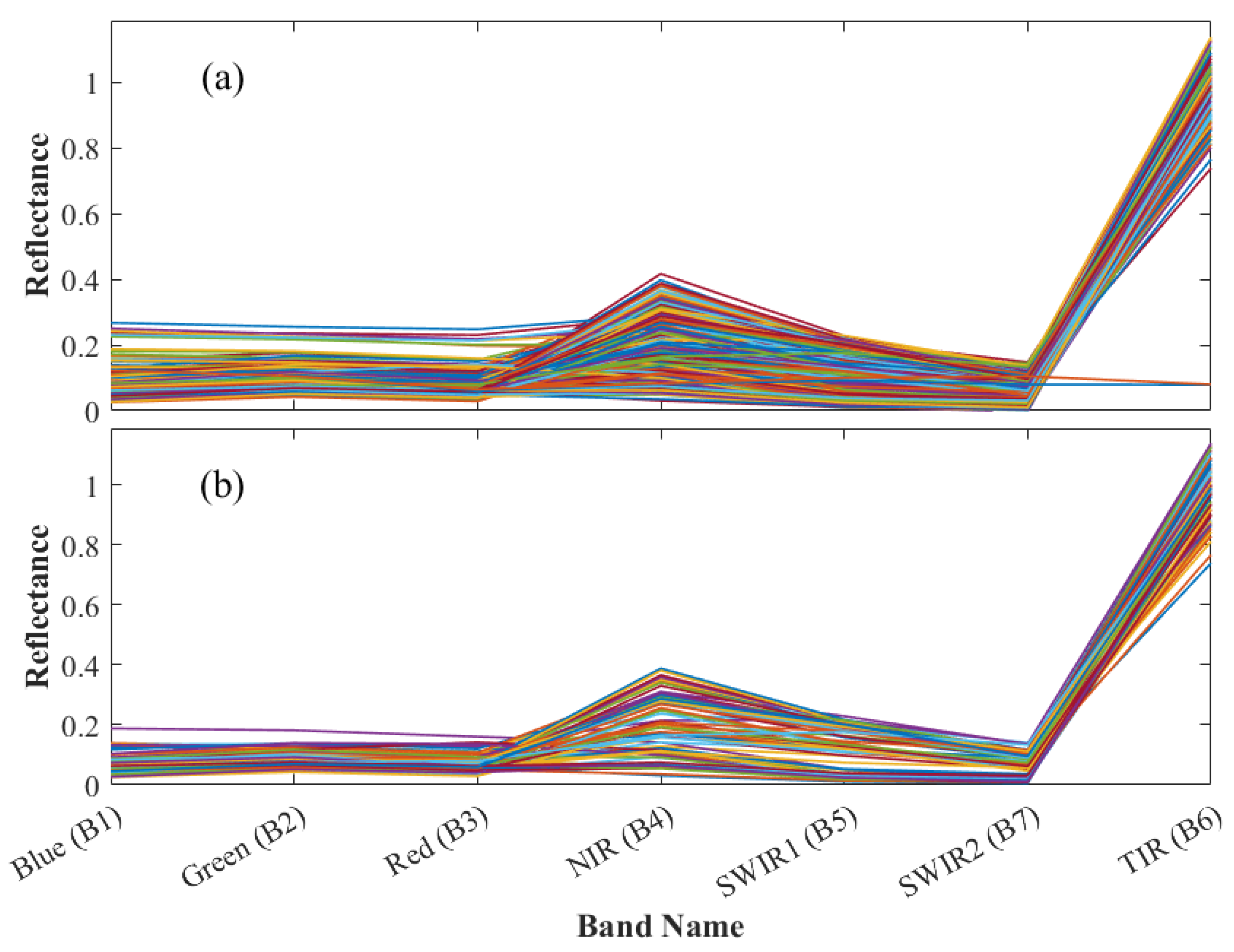
Water bodies in differing trophic states exhibit distinct absorption, scattering, and transmission responses across spectral bands [39]. To evaluate their optical characteristics and quantify the impact of preprocessing, we plotted spectral reflectance curves from Landsat 5 imagery before and after correction. Figure 6a shows the raw spectral profile, which contains anomalous fluctuations, whereas Figure 6b displays the atmospherically corrected profile, exhibiting a consistent spectral trend.

3.3. TSI Inversion Prediction Model Based on BP-NN-GSA

3.3.1. Architecture of the Backpropagation Neural Network Model

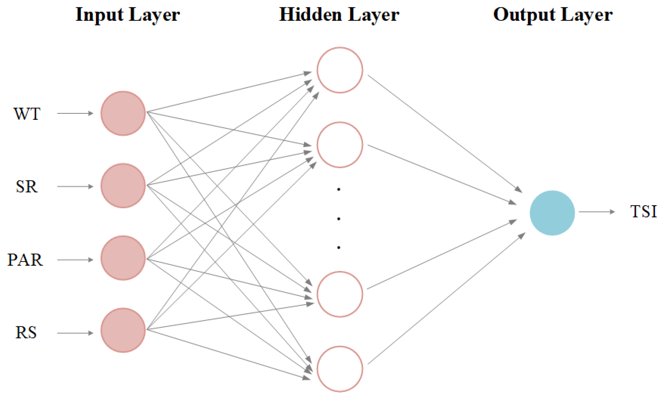
The BP-NN is a multilayer feedforward network that adaptively learns complex nonlinear mappings without manual weight tuning, thereby enhancing the precision and applicability of water quality assessments. Its architecture consists of an input layer, a hidden layer and an output layer, where state variations in the hidden layer modulate the mapping between inputs and outputs. In this study, we implemented a three layer BP-NN inversion model for trophic state estimation (Figure 7) [40].

3.3.2. Model Parameters

We configured the BP-NN to train for 10,000 iterations while all other hyperparameters were optimized via grid search. The momentum factor was varied from 0.7 to 0.9 in steps of 0.05. The learning rate ranged from 0.0005 to 0.01 with a step size of 0.001. Early-stopping patience (maximum failures) was set between 6 and 15, in increments of 1. A detailed grid search across these ranges found optimal performance on the training set at a learning rate of 0.0095, a momentum factor of 0.9 and a patience of 15. To mitigate overfitting, we partitioned the dataset randomly into 70% for training, 15% for validation, and 15% for testing, thereby ensuring a robust assessment of generalization error.
Grid search entails discretizing the hyperparameter domain into a structured grid, systematically evaluating the objective function at each node subject to constraint functions, and selecting the configuration that optimizes model performance (Figure 8) [41]. In this investigation, we defined hyperparameter ranges and grid resolutions, then conducted an exhaustive search across all grid points to identify the combination that maximized model accuracy. Upon convergence, the search terminated and the optimal hyperparameter values were extracted. This procedure was employed to fine-tune the model’s parameters, thereby enhancing its predictive precision.

3.3.3. Performance Evaluation of the BP-NN-GSA Model

In the performance evaluation of water quality remote sensing inversion models, multiple statistical metrics are routinely employed to comprehensively quantify model goodness-of-fit and error characteristics. In this study, three such indicators—the coefficient of determination (R2), root mean square error (RMSE) and mean absolute percentage error (MAPE)—are adopted to systematically assess the robustness, absolute accuracy, and relative error of the proposed model across datasets with varying spatial and temporal scales [23,42]. Among these, R2 directly quantifies the proportion of variance in in situ measurements explained by the model-derived values and is therefore designated as the primary metric for evaluating inversion accuracy.
The coefficient of R2 measures the correlation between observed and predicted values from the model inversion. Its value ranges from 0 to 1, with a value closer to 1 indicating better model performance. The formula for its calculation is as follows:
R 2 = 1 i = 1 a ( t i y i ) 2 i = 1 a ( t i t ¯ ) 2
where t i represents the observed TSI value for the i-th sample; y i represents the predicted TSI value for the i-th sample; and a denotes the model’s training dataset.
The RMSE quantifies the deviation between observed and predicted values by computing the square root of the mean of squared residuals, thereby penalizing larger deviations more heavily and effectively highlighting outliers. The formula for its computation is as follows:
RMSE = 1 n i = 1 a ( t i y i ) 2
The MAPE computes the average relative error between observed and predicted values, normalizing by TSI magnitude to yield a scale-independent assessment of model credibility; a higher MAPE indicates larger errors. The formula for its computation is as follows:
MAPE = 100 a × i = 1 a t i y i t i

4. Results

4.1. Comparison of TSI Inversion Accuracy for Different Parameter Combinations

We configured the BP-NN with seven hidden neurons and optimized it using GSA to enhance model accuracy. Environmental factors were selected via Pearson correlation analysis and, together with spectral band reflectance data, formed six distinct input variable combinations.
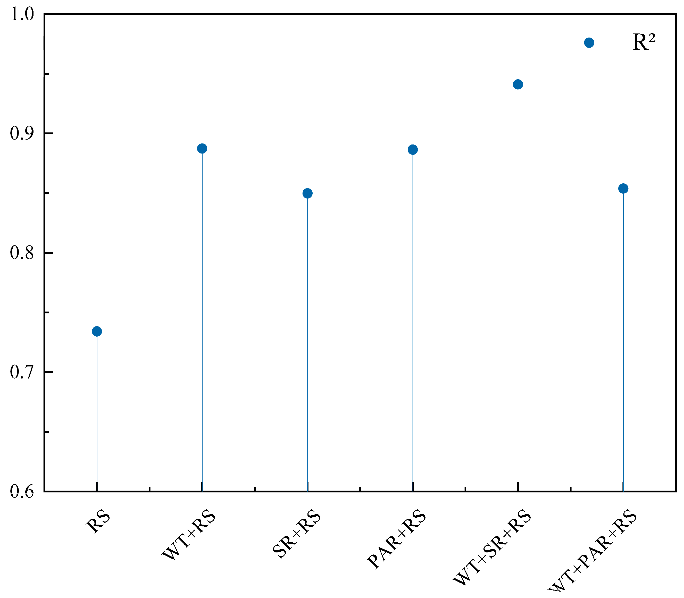
This study evaluated model performance using the R2, RMSE, and MAPE. The WT, SR and RS combination achieved the highest R2 (0.94) (Figure 9), while also recording the lowest RMSE (3.588) and MAPE (2.562) among all tested configurations. Based on this comprehensive three-metric assessment, the WT, SR and RS combination was selected as the optimal set of input variables.

4.2. Evaluation of the Accuracy of the TSI Inversion Model

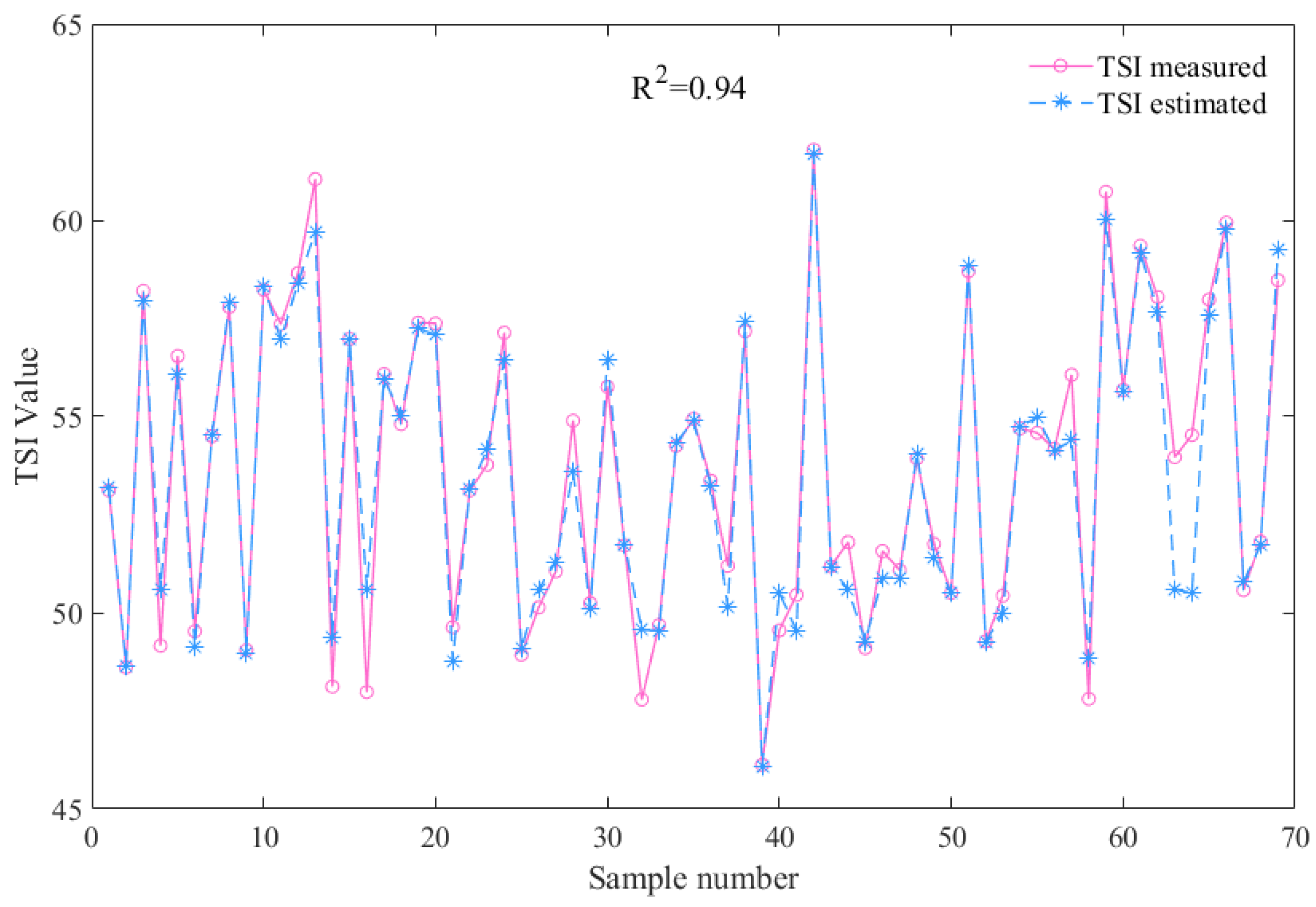
We randomly allocated 70% of the dataset to model training and ultimately identified WT, SR and RS together as the optimal input combination. Figure 10 presents a scatter plot of measured versus predicted TSI values for the WT, SR and RS configuration during training (R2 = 0.94), illustrating the model’s strong predictive performance.
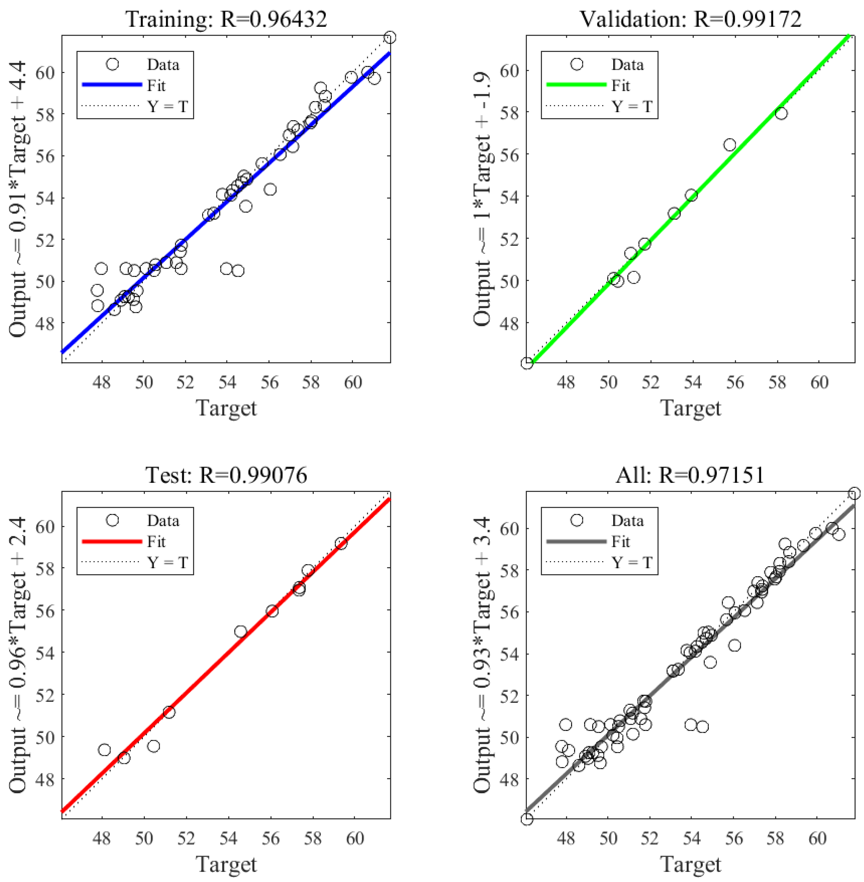
Early stopping halted training at epoch 15, once the validation error stopped decreasing, preventing overfitting. Regression plots in Figure 11 show high R2 values for the training (0.9643), validation (0.9917) and test (0.9908) sets. Notably, validation and test R2 exceed the training R2, unlike typical overfitting patterns. These metrics indicate no evident overfitting and strong generalization.

4.3. Prediction of Spatiotemporal Distribution of TSI

We accessed remote sensing imagery of Xiangxi Bay for specified times and regions using GEE. Because heavy cloud cover often compromises image usability, we selected high-quality scenes with minimal cloud contamination for preprocessing prior to download and predictive analysis.

4.3.1. Prediction of TSI for 2009

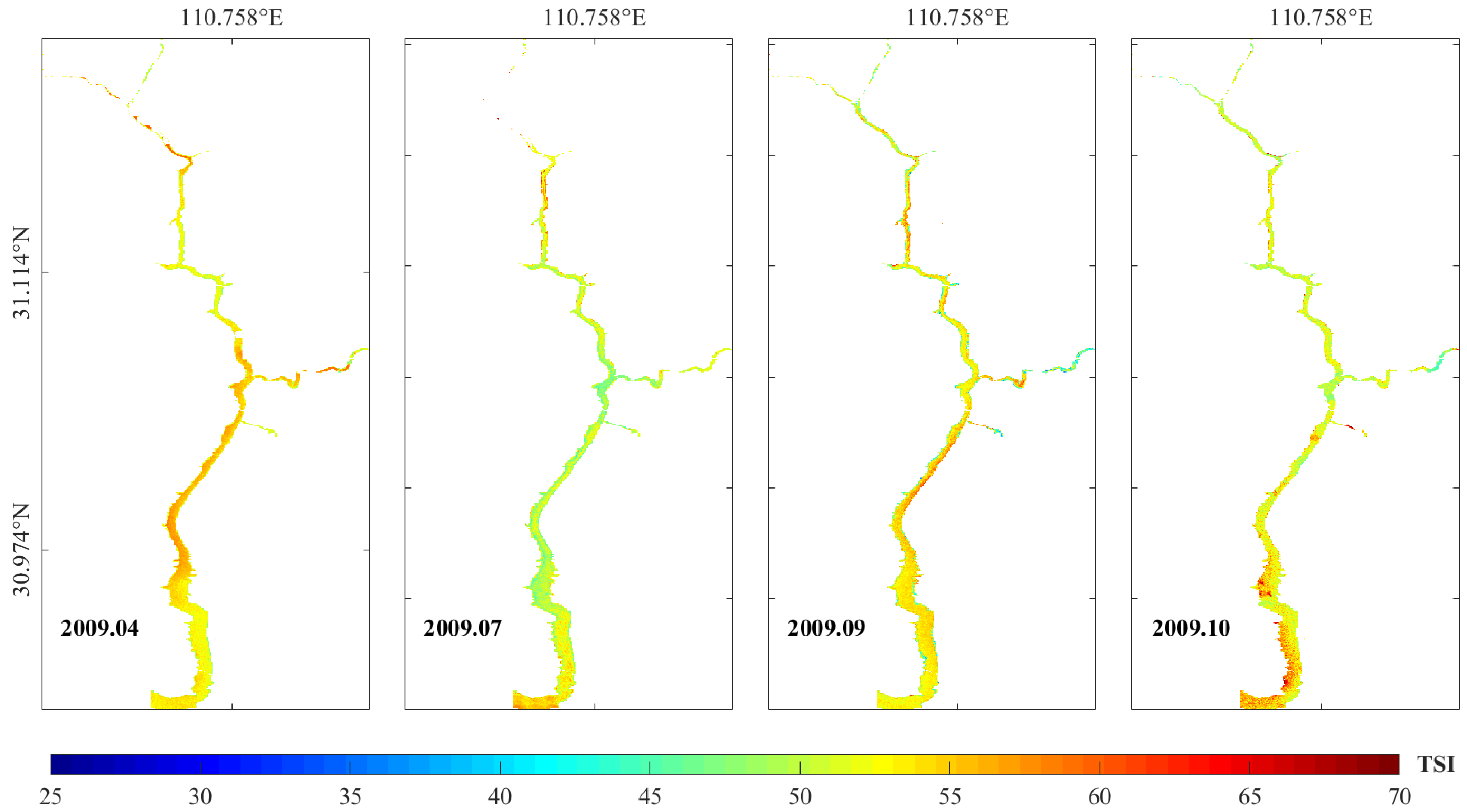
We fused the top-performing environmental predictors (WT, SR and RS) with Landsat 5’s seven spectral bands into a raster stack, which we then fed into the trained BP-NN-GSA model to predict TSI values for each pixel and generate spatiotemporal distribution maps. We input remote sensing scenes from April, July, September, and October 2009 into the BP-NN-GSA model for TSI inversion, generating spatiotemporal distribution maps (Figure 12) that illustrate TSI’s temporal progression and spatial variability in Xiangxi Bay waters.
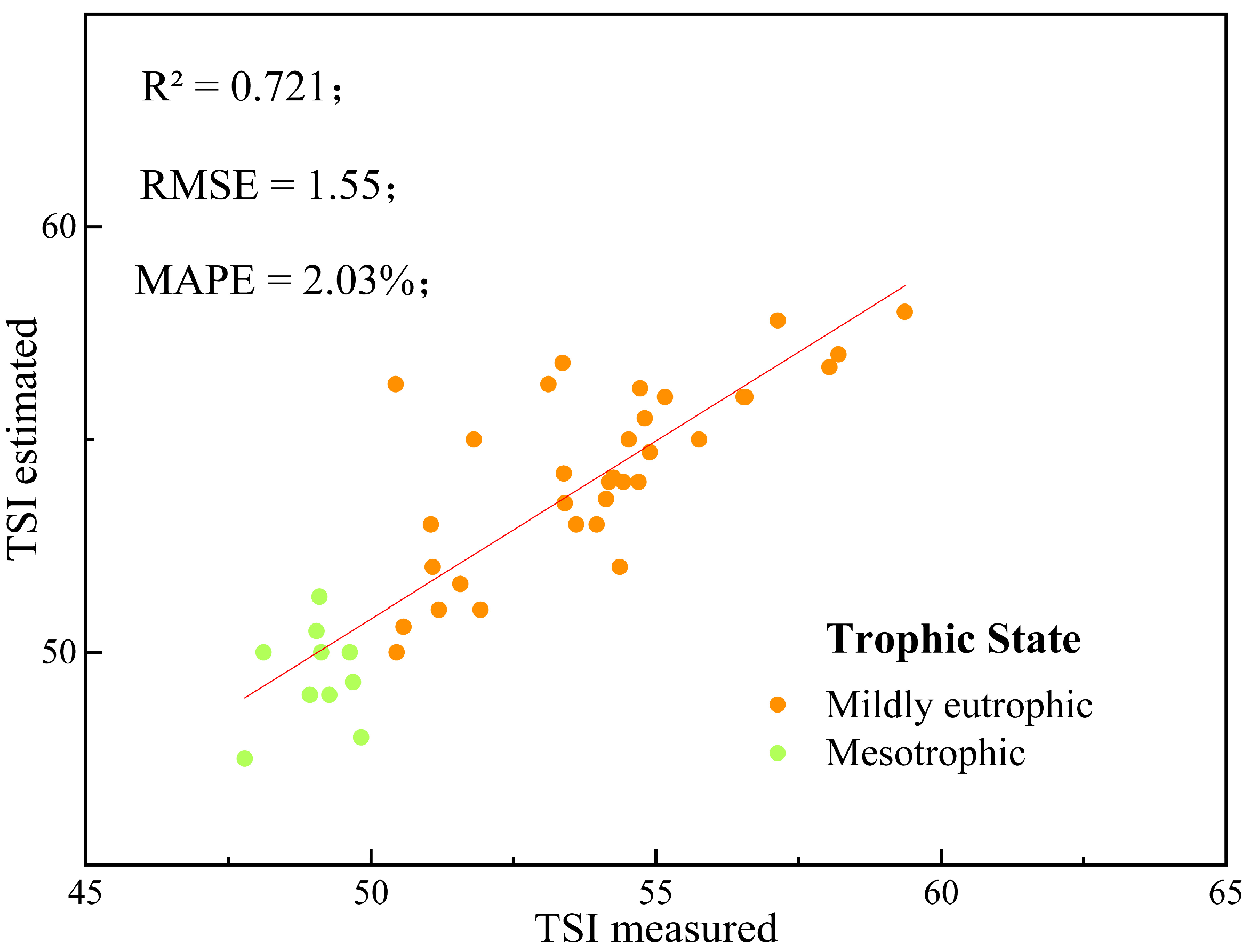
TSI inversion results for Xiangxi Bay indicate that trophic status values in April and September were generally higher than those in July and October (Figure 12). The April peak likely reflects rising spring temperatures, increased aquatic biological activity, and accelerated metabolism. Predicted TSI values at 11 monitoring sites for 2009 were compared with measurements via a scatter plot (Figure 13), yielding R2 = 0.721, RMSE = 1.55 and MAPE = 2.03%, which demonstrates good agreement between predictions and observations. Across the four simulated maps, temporal TSI trajectories at the eleven monitoring stations closely mirror measured trends, attesting to the model’s feasibility and commendable predictive accuracy. In the July and September outputs, several reaches near boundaries display locally elevated predicted TSI values. These anomalies may be attributed to the combined effects of higher summer temperatures and substantial domestic wastewater inputs from neighboring villages, which together create more complex boundary-layer environments and render these marginal zones especially vulnerable to anthropogenic influences.
Moreover, the elongated planform of Xiangxi Bay gives rise to a pronounced longitudinal gradient in trophic status. Overall, the middle and downstream reaches are more eutrophic than the upper section. Dense clusters of villages along these middle and downstream reaches, combined with substantial agricultural return flows, intensify anthropogenic disturbances, accelerate algal proliferation, and consequently elevate TSI values. TSI is further increased within weakly flushed embayments, where reduced hydrodynamic scouring promotes the retention of nutrients and algae compared to adjoining open-water areas.

4.3.2. TSI Prediction for 2019 and 2020

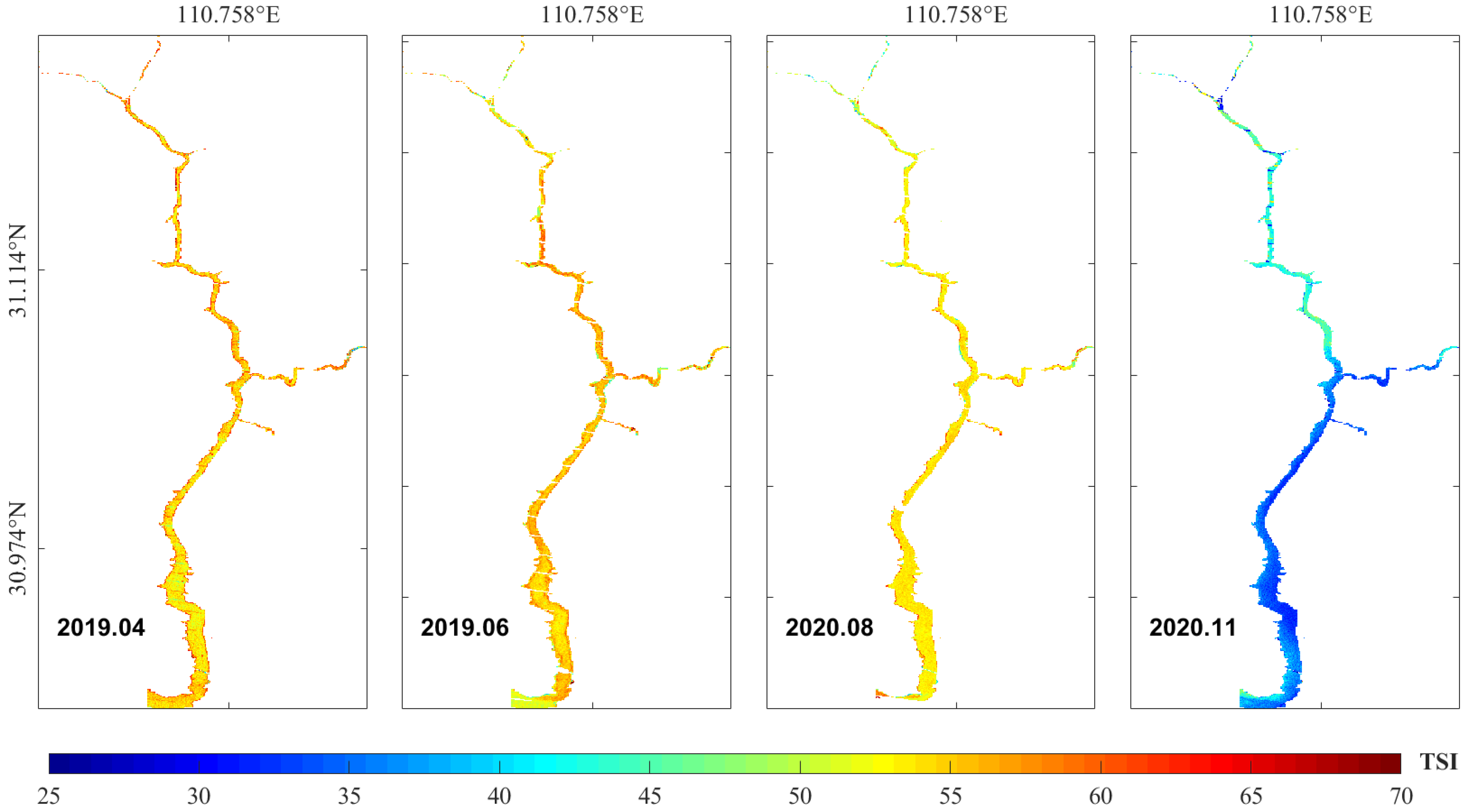
We evaluated the model’s performance by selecting Landsat 7 scenes acquired along the original training timeline for TSI inversion. Drawing on the 2009 simulation outcomes where summer conditions (higher temperatures, extended photoperiods, and increased precipitation) and intensified anthropogenic and agro-industrial influences exacerbated nutrient levels, we identified four seasonally representative months based on scene quality: April and June 2019, and August and November 2020. These scenes were preprocessed and fed into the trained inversion model (Figure 14).
Analysis of the 2019 and 2020 TSI prediction maps indicates that the simulated TSI values for April, June and August exceed those for November, mirroring the pattern observed in the 2009 results and thereby corroborating the model’s robustness (Figure 14). The summertime increase is plausibly driven by higher ambient temperatures, extended photoperiods, and increased rainfall, all of which enhance nutrient influx and stimulate algal growth. In contrast, November exhibits the lowest TSI estimates among the four study months; this decline coincides with cooler temperatures, reduced daylight, and a general decrease in anthropogenic activity along Xiangxi Bay, collectively diminishing external disturbances and nutrient loading.
The August prediction map likewise reveals isolated river reaches where estimated TSI values are comparatively higher at watershed boundaries. These localized anomalies are most plausibly attributed to elevated summer temperatures and intensified anthropogenic inputs from neighboring villages, which together create a more complex boundary-layer environment and distinguish the trophic status of marginal waters from that of the mid-channel. The spatiotemporal TSI map for Xiangxi Bay shows elevated values in April 2019, emphasizing the effects of climate change and spring biological recovery on water quality.

5. Discussion

We developed a TSI remote sensing inversion model that integrates environmental variables, water quality metrics, and satellite imagery to accurately characterize nutrient status and its spatiotemporal patterns in Xiangxi Bay. Our results demonstrate that nutrient dynamics closely correlate with natural drivers (WT and SR), anthropogenic pressures, and agro-industrial activities [33,43]. Specifically, TSI values peak in summer relative to spring and winter, and boundary zones—where human intervention is most intensive—exhibit distinct TSI signatures compared to interior reaches, underscoring pronounced spatiotemporal heterogeneity.
WT is a critical driver of complex spatiotemporal water quality dynamics [44]. Our findings indicate that, in addition to the summertime peak, Xiangxi Bay is also highly susceptible to algal bloom occurrences in spring. Since the impoundment of the Three Gorges Reservoir, the resultant increase in water level and the reduction in flow velocity have promoted nutrient retention within tributary embayments. Pronounced thermal contrasts between the main stem and its tributaries generate density-driven underflows, transporting nutrient-rich water into these semi-enclosed bays where it accumulates. When suitable thermal conditions prevail, these processes make the tributary embayments of the Three Gorges system, particularly Xiangxi Bay, especially prone to algal bloom outbreaks [45,46]. Accordingly, water quality monitoring in Xiangxi Bay should prioritize the spring season, where management objectives and field conditions allow, to increase the sampling frequency.
Our results indicate that trophic conditions in summer are poorer than those in spring or winter. The principal drivers are the higher air temperatures, abundant rainfall, and intense solar radiation characteristic of the local summer climate [33]. These factors accelerate nutrient delivery to Xiangxi Bay via surface runoff, enhance biochemical activity, stimulate algal growth, and ultimately elevate the overall trophic level. Consequently, the observed seasonal pattern in water quality broadly reflects the region’s topographic and climatic setting [26]. Localized TSI anomalies at watershed margins can be attributed to the intrinsic complexity of inland waters, where heterogeneity in water quality parameters and in the absorption and scattering properties of optically active substances, along with their concentration-dependent spectral signatures, produces pronounced boundary effects [39,47].
TSI values are also higher in weakly flushed embayments than in adjacent open waters, most likely because impoundment by the Three Gorges Reservoir has raised water levels, reduced flow velocities, and hindered the downstream transport of algae and nutrients [48]. In our 2019 simulations, a propensity for spring algal blooms emerges. We attribute this to nutrient accumulation in embayments under low-flow conditions and to density-driven currents induced by significant temperature gradients between the main stem and its tributaries; these currents transport nutrient-rich water into the bays. When such processes coincide with suitable temperatures, tributaries of the Three Gorges System, particularly Xiangxi Bay, become highly susceptible to bloom outbreaks [45,46]. Operational rules of the Three Gorges Reservoir were revised in 2015 and 2019, raising flood-limited water levels during the flood season and moving the start of storage to September. This policy shift affects water quality and adds uncertainty to the retrieval model’s accuracy [49]. Given current data constraints, the 2019–2020 predictions serve primarily as preliminary tests of model applicability under these changing management conditions.
The standard empirical TSI formulas based on Chl-a, TP and TN were developed for broader, more stable water bodies and do not capture the complex hydrodynamics of narrow, dynamic tributaries like Xiangxi Bay [50]. Applying them here may introduce bias, particularly since our dataset lacks extreme oligotrophic or hypereutrophic cases and cannot span the full TSI range [51]. In tributary settings with pronounced hydrodynamic processes, future work should include targeted in situ monitoring to recalibrate or adjust TSI parameters, thereby improving both accuracy and adaptability. This represents a key direction for further research.
This inversion model utilizes a BP neural network in conjunction with a GSA to optimize its parameters, thereby improving the accuracy of TSI inversion and prediction while eliminating the substantial time and effort required for manual tuning. The model accepts various combinations of environmental drivers, in situ water quality measurements, and satellite remote sensing data as inputs, with the TSI value as the output. Compared to traditional approaches that invert only a single factor, this integrated framework enables a more holistic and comprehensive assessment of the trophic status in Xiangxi Bay [52].
Several limitations warrant consideration. First, the non-repetitive random split into 70/15/15 training/validation/test subsets can produce unstable partitions when each group contains few samples. Repeated cross-validation or bootstrap resampling would yield more reliable error estimates [53]. Second, TSI predictions are highly sensitive to input data uncertainty, particularly in remote sensing reflectance and meteorological measurements. Atmospheric interference, sensor error and timing mismatches can introduce noise or bias that propagates through the model [54]. Moreover, cloud cover, especially during the humid season, reduces the completeness of satellite imagery, creating data gaps [55]. Although manual screening, atmospheric correction and radiometric calibration help mitigate these effects, residual uncertainties may still compromise model robustness in certain regions or periods. Finally, applying an IQR-based outlier filter removes physically implausible values but may also discard rare yet valid observations when sample sizes are small. Future work could adopt robust regression or ensemble modeling approaches to handle outliers more effectively without manual exclusion.
We note that neural networks necessitate extensive training data [56]; however, our dataset currently omits samples classified as oligotrophic (TSI < 30) and hyper-eutrophic (TSI > 70), limiting model coverage. Future work will augment the training corpus with threshold-defined TSI classes to enhance the inversion model’s comprehensiveness and predictive accuracy. Given the small training dataset, overfitting remains a concern. Future work should include independent validation datasets from other regions or years and assess performance across diverse environmental and sensing conditions to improve generalizability.

6. Conclusions

We developed a BP-NN-GSA inversion model that integrates multi-source data. The model jointly considers environmental drivers and water quality indicators, using satellite remote sensing imagery and in situ measurements as inputs (n = 98). Model hyperparameters were optimized with the GSA, yielding a marked accuracy improvement (R2 = 0.94). The model effectively reproduces the spatiotemporal distribution of the TSI across four representative months in 2009 for Xiangxi Bay—a river-type tributary bay formed by the impoundment of the Three Gorges Reservoir. The results reveal pronounced spatiotemporal fluctuations in the TSI and highlight the substantial influence of surrounding environmental factors. By fusing remote sensing features with environmental variables, the approach mitigates data sparsity and provides a broader pathway for future water quality retrieval modeling.
Using Landsat 5 and 7 surface reflectance data, we trained a model to predict/retrieve TSI in Xiangxi Bay circa 2012 with application-level accuracy. Performance was evaluated using R2, RMSE, and MAPE. With the optimal input combination of WT, SR, and RS, the model achieved an R2 of 0.94, an RMSE of 3.588, and a MAPE of 2.562%. For 2009, the predicted TSI values were extracted and compared with in situ observations, yielding R2 = 0.721. We further generated out-of-period predictions for April and June 2019 and August and November 2020 to provide an initial assessment of model applicability beyond the training window. The fusion of multi-source data relaxes limitations inherent to single-source remote sensing, alleviates data scarcity, and demonstrates substantial potential, offering a basis for subsequent research.
Overall, remote sensing-based inversion achieves high accuracy for reservoir tributary bays and is applicable to river-type bays in large reservoirs. Future work should expand the sample set—particularly including extreme water quality scenarios—and incorporate these cases into training to reduce model limitations and improve robustness. Adopting optimization algorithms with parameters tailored to this setting may further enhance generalization, mitigate edge effect issues in retrievals, and improve the accuracy of algal bloom predictions.

Author Contributions

Conceptualization, Y.S., J.M. and D.M.; methodology, Y.S. and J.Z.; software, Y.S., J.Z. and H.G.; validation, Y.S. and K.W.; formal analysis, Y.S. and X.L.; investigation, Y.S. and K.W.; resources, J.M.; data curation, Y.S. and J.M.; writing—original draft preparation, Y.S.; writing—review and editing, Y.S., J.M., H.G., K.W., D.M. and J.Z.; visualization, Y.S. and X.L.; supervision, J.M. and X.L.; project administration, J.M.; funding acquisition, J.M. and X.L. All authors have read and agreed to the published version of the manuscript.

Funding

This research was funded by the National Natural Science Foundation of China (52279013); Hubei Provincial Natural Science Foundation of China (2023AFD201); China Yangtze Power Co., Ltd. Research Project (Z242302063).

Data Availability Statement

The data presented in this study is available on request from the corresponding author. The data are not publicly available due to the fact that it is currently privileged information.

Acknowledgments

The authors would like to thank the anonymous reviewers for their constructive comments and suggestions, which greatly improved this paper.

Conflicts of Interest

Author Xinbo Liu was employed by the company China Yangtze Power Co., Ltd. The remaining authors declare that the research was conducted in the absence of any commercial or financial relationships that could be construed as a potential conflict of interest.

References

  1. Zhao, C.M.; Dong, X.H.; Li, Z.H.; Bo, H.J.; Zhang, Q.Y.; Zhang, C.Y. Remote Sensing Retrieval of Water Quality in the East Tributary of Huangbaihe River Based on Neural Networks. Environ. Sci. Technol. 2022, 45, 195–202. [Google Scholar]
  2. Bricker, S.B.; Longstaff, B.; Dennison, W.; Jones, A.; Boicourt, K.; Wicks, C.; Woerner, J. Effects of Nutrient Enrichment in the Nation’s Estuaries: A Decade of Change. Harmful Algae 2008, 8, 21–32. [Google Scholar] [CrossRef]
  3. Le Gall, M.; Evrard, O.; Foucher, A.; Laceby, J.; Salvador-Blanes, S.; Thil, F.; Dapoigny, A.; Lefèvre, I.; Cerdan, O.; Ayrault, S. Quantifying Sediment Sources in a Lowland Agricultural Catchment Pond Using 137Cs Activities and Radiogenic 87Sr/86Sr Ratios. Sci. Total Environ. 2016, 566, 968–980. [Google Scholar] [CrossRef]
  4. Hallegraeff, G.; Enevoldsen, H.; Zingone, A. Global Harmful Algal Bloom Status Reporting. Harmful Algae 2021, 102, 101992. [Google Scholar] [CrossRef] [PubMed]
  5. Liu, X.; Huang, W.; Qi, Z.X.; Li, C.B.; Cheng, G.H.; Cai, Y.P. Seasonal Water Storage of Large Reservoirs Exacerbates Eutrophication Risk in the Fluctuating Backwater Zone: A Case Study of Three Gorges Reservoir, China. Ecol. Indic. 2025, 171, 113100. [Google Scholar] [CrossRef]
  6. Yang, L.; Liu, D.; Huang, Y.; Yang, Z.; Ji, D.; Song, L. Isotope Analysis of the Nutrient Supply in Xiangxi Bay of the Three Gorges Reservoir. Ecol. Eng. 2015, 77, 65–73. [Google Scholar] [CrossRef]
  7. Barnieh, B.A.; Davis, C. Monitoring Anthropogenic Impacts on Water Quality in Ghana with Remote Sensing. Nat. Rev. Earth Environ. 2025, 6, 378. [Google Scholar] [CrossRef]
  8. Pu, M.Y.; Xu, J.Q.; Hu, K.Y.; Peng, K.; Gong, Z.; Cai, Y.J.; Xiang, X.L. Community structure and driving factors of zooplankton in the littoral zone of Lake Hongze. J. Lake Sci. 2023, 35, 610–621. [Google Scholar] [CrossRef]
  9. Gordon, H.R.; Wang, M. Retrieval of Water-Leaving Radiance and Aerosol Optical Thickness over the Oceans with SeaWiFS: A Preliminary Algorithm. Appl. Opt. 1994, 33, 443. [Google Scholar] [CrossRef]
  10. Ramaraj, M.; Sivakumar, R. Remote Sensing and Nonlinear Auto-Regressive Neural Network (NARNET) Based Surface Water Chemical Quality Study: A Spatio-Temporal Hybrid Novel Technique (STHNT). Bull. Environ. Contam. Toxicol. 2022, 110, 28. [Google Scholar] [CrossRef]
  11. Qiao, Z.; Sun, S.Y.; Jiang, Q.O.; Xiao, L.; Wang, Y.Q.; Yan, H.M. Retrieval of Total Phosphorus Concentration in the Surface Water of Miyun Reservoir Based on Remote Sensing Data and Machine Learning Algorithms. Remote Sens. 2021, 13, 4662. [Google Scholar] [CrossRef]
  12. Zhang, F.; Xue, B.; Cai, Y.; Xu, H.; Zou, W. Utility of Trophic State Index in Lakes and Reservoirs in the Chinese Eastern Plains Ecoregion: The Key Role of Water Depth. Ecol. Indic. 2023, 148, 110029. [Google Scholar] [CrossRef]
  13. Palmer, C.J.; Kutser, T.; Hunter, P.D. Remote Sensing of Inland Waters: Challenges, Progress and Future Directions. Remote Sens. Environ. 2015, 157, 1–8. [Google Scholar] [CrossRef]
  14. Hu, M.; Wang, Y.; Sun, Z.; Su, Y.; Li, S.; Bao, Y.; Wen, J. Performance of Ensemble-Learning Models for Predicting Eutrophication in Zhuyi Bay, Three Gorges Reservoir. River Res. Appl. 2021, 37, 1104–1114. [Google Scholar] [CrossRef]
  15. Sun, Y.; Wang, D.H.; Li, L.; Ning, R.S.; Yu, S.; Gao, N.Y. Application of Remote Sensing Technology in Water Quality Monitoring: From Traditional Approaches to Artificial Intelligence. Water Res. 2024, 267, 122546. [Google Scholar] [CrossRef] [PubMed]
  16. Yang, H.B.; Kong, J.L.; Hu, H.H.; Du, Y.; Gao, M.Y.; Chen, F. A Review of Remote Sensing for Water Quality Retrieval: Progress and Challenges. Remote Sens. 2022, 14, 1770. [Google Scholar] [CrossRef]
  17. Ding, H.; Li, R.R.; Lin, H.; Wang, X. Monitoring and Evaluation on Water Quality of Hun River Based on Landsat Satellite Data. In Proceedings of the 2016 Progress in Electromagnetic Research Symposium (PIERS), Shanghai, China, 8–11 August 2016; IEEE: Shanghai, China, 2016; pp. 1532–1537. [Google Scholar]
  18. Tesfaye, M.; Breuer, L. Remote Sensing with Machine Learning for Multi-Decadal Surface Water Monitoring in Ethiopia. Sci. Rep. 2025, 15, 12444. [Google Scholar] [CrossRef]
  19. He, Y.H.; Gong, Z.J.; Zheng, Y.H.; Zhang, Y.B. Inland Reservoir Water Quality Inversion and Eutrophication Evaluation Using BP Neural Network and Remote Sensing Imagery: A Case Study of Dashahe Reservoir. Water 2021, 13, 2844. [Google Scholar] [CrossRef]
  20. Cao, Q.; Yu, G.L.; Sun, S.J.; Dou, Y.; Li, H.; Qiao, Z.Y. Monitoring Water Quality of the Haihe River Based on Ground-Based Hyperspectral Remote Sensing. Water 2022, 14, 22. [Google Scholar] [CrossRef]
  21. Wang, X.C.; Cui, J.; Xu, M.M. A Chlorophyll-a Concentration Inversion Model Based on Backpropagation Neural Network Optimized by an Improved Metaheuristic Algorithm. Remote Sens. 2024, 16, 1503. [Google Scholar] [CrossRef]
  22. Guo, Q.Z.; Wu, H.; Jin, H.Y.; Yang, G.; Wu, X.X. Remote Sensing Inversion of Suspended Matter Concentration Using a Neural Network Model Optimized by the Partial Least Squares and Particle Swarm Optimization Algorithms. Sustainability 2022, 14, 2221. [Google Scholar] [CrossRef]
  23. Meng, D.H.; Mao, J.Q.; Li, W.F.; Zhu, S.J.; Gao, H. An Integrated Framework for Remote Sensing Assessment of the Trophic State of Large Lakes. Remote Sens. 2023, 15, 4238. [Google Scholar] [CrossRef]
  24. Jiang, D.G.; Dai, H.C.; Wang, W.; Liu, W. Causing Analysis on Nutrients Spatial Difference in Xiangxi Bay of the Three Gorges Reservoir. J. Hydraul. Eng. 2013, 44, 562–569. [Google Scholar]
  25. Tang, H.; Yu, Y.; Yuan, S.; Li, Z.; Cao, H.; Jiang, C.; Gualtieri, C. Hydrodynamics and Sediment Transport in Poyang Lake under the Effects of Wind and Backflow. Hydrol. Res. 2023, 54, 1281–1298. [Google Scholar] [CrossRef]
  26. Deng, L.; Li, W.S.; Liu, X.J.; Wang, Y.Z.; Wang, L.Q. Landscape Patterns and Topographic Features Affect Seasonal River Water Quality at Catchment and Buffer Scales. Remote Sens. 2023, 15, 1438. [Google Scholar] [CrossRef]
  27. Zhou, B.; Shi, K.; Wang, W.; Zhang, D.; Qin, B.; Zhang, Y.; Dong, B.; Shang, M. Phytoplankton Succession Phenology Trends in the Backwaters of the Three Gorges Reservoir in China and Their Drivers: Results from Satellite Observations. Ecol. Indic. 2022, 143, 109435. [Google Scholar] [CrossRef]
  28. Hasan, B.M.S.; Abdulazeez, A.M. A Review of Principal Component Analysis Algorithm for Dimensionality Reduction. J. Soft Comput. Data Min. 2021, 2, 20–30. [Google Scholar] [CrossRef]
  29. Lu, W.K.; Yu, L.X.; Ou, X.K.; Li, F.L. Relationship between Occurrence Frequency of Cyanobacteria Bloom and Meteorological Factors in Lake Dianchi. J. Lake Sci. 2017, 29, 534–545. [Google Scholar] [CrossRef]
  30. Xenopoulos, M.; Frost, P.; Elser, J. Joint Effects of UV Radiation and Phosphorus Supply on Algal Growth Rate and Elemental Composition. Ecology 2002, 83, 423–435. [Google Scholar] [CrossRef]
  31. Ni, M.F.; Ge, Q.S.; Li, S.Y.; Wang, Z.K.; Wu, Y.J. Trophic State Index Linked to Partial Pressure of Aquatic Carbon Dioxide in a Typical Karst Plateau Lake. Ecol. Indic. 2021, 120, 106912. [Google Scholar] [CrossRef]
  32. Efimova, T.; Churilova, T.; Skorokhod, E.; Buchelnikova, V.; Buchelnikov, A.; Moiseeva, N.; Salyuk, P.; Stepochkin, I.; Melnik, A. Effect of Water Trophic Status on Bio-Optical Properties and Productive Characteristics of Phytoplankton of the Black Sea Coastal Waters near Sevastopol. Mar. Biol. Res. 2023, 19, 81–93. [Google Scholar] [CrossRef]
  33. Wen, Z.; Song, K.; Fang, C.; Yang, Q.; Liu, G.; Shang, Y.; Wang, X. Estimation of Kd(PAR) in Inland Waters across China in Relation to the Light Absorption of Optically Active Components. Environ. Sci. Pollut. Res. 2019, 26, 30098–30111. [Google Scholar] [CrossRef]
  34. Zhu, S.J.; Mao, J.Q. A Machine Learning Approach for Estimating the Trophic State of Urban Waters Based on Remote Sensing and Environmental Factors. Remote Sens. 2021, 13, 2498. [Google Scholar] [CrossRef]
  35. Koda, S.; Zeggada, A.; Melgani, F.; Nishii, R. Spatial and Structured SVM for Multilabel Image Classification. IEEE Trans. Geosci. Remote Sens. 2018, 56, 5948–5960. [Google Scholar] [CrossRef]
  36. Xue, K.; Zhang, Y.C.; Duan, H.T.; Ma, R.H. Variability of Light Absorption Properties in Optically Complex Inland Waters of Lake Chaohu, China. J. Great Lakes Res. 2017, 43, 17–31. [Google Scholar] [CrossRef]
  37. Shu, Y. Comparative Analysis on Outlier Elimination Methods for GPS Coordinate Time Series. J. Navig. Position. 2021, 9, 79–85. [Google Scholar]
  38. Yue, H.; Li, Y.; Qian, J.X.; Liu, Y. A New Accuracy Evaluation Method for Water Body Extraction. Int. J. Remote Sens. 2020, 41, 7311–7342. [Google Scholar] [CrossRef]
  39. Shi, K.; Li, Y.M.; Li, L.; Lu, H. Absorption Characteristics of Optically Complex Inland Waters: Implications for Water Optical Classification. J. Geophys. Res. Biogeosci. 2013, 118, 860–874. [Google Scholar] [CrossRef]
  40. Meng, D.H.; Mao, J.Q.; Li, W.F.; Gao, H.; Sheng, L.Y. Remote Sensing Assessment of Trophic State of Large Lakes by Integrating Multi-Source Information. J. Hydroelectr. Eng. 2024, 43, 13–23. [Google Scholar]
  41. Wen, B.W.; Dong, W.H.; Xie, W.J.; Ma, J. Parameter Optimization Method for Random Forest Based on Improved Grid Search Algorithm. Comput. Eng. Appl. 2018, 54, 154–157. [Google Scholar]
  42. Wang, J.; Shi, T.; Yu, D.; Teng, D.; Ge, X.; Zhang, Z.; Yang, X.; Wang, H.; Wu, G. Ensemble Machine-Learning-Based Framework for Estimating Total Nitrogen Concentration in Water Using Drone-Borne Hyperspectral Imagery of Emergent Plants: A Case Study in an Arid Oasis, NW China. Environ. Pollut. 2020, 266, 115412. [Google Scholar] [CrossRef]
  43. Guan, Q.; Tang, J.; Feng, L.; Olin, S.; Schurgers, G. Long-Term Changes of Nitrogen Leaching and the Contributions of Terrestrialnutrient Sources to Lake Eutrophication Dynamics on the Yangtze Plain of China. Biogeosciences 2023, 20, 1635–1648. [Google Scholar] [CrossRef]
  44. Wang, D.Y.; Feng, X.Z.; Zhou, L.G.; Hao, J.Y.; Xu, X.X. Relationship between Blue Algal Bloom and Water Temperature in Lake Taihu Based on MODIS. Sci. Limnol. Sin. 2008, 20, 173–178. [Google Scholar]
  45. Jiang, D.G.; Dai, H.C.; Liu, W. Temporal and Spatial Distributions of Nutrients in Xiangxi Bay of the Three Gorges Reservoir under the Influence of Temperature Density Current. J. Basic Sci. Eng. 2013, 21, 20–31. [Google Scholar]
  46. Zhang, J.; Ye, D.; Zhu, H.T.; Hu, S.; Wang, Y.C.; Tang, J.F.; Zhou, Z. Characteristics of Spring Algal Blooms under Different Impounded Levels in Tributaries of the Three Gorges Reservoir. Acta Hydrobiol. Sin. 2019, 43, 884–891. [Google Scholar]
  47. Baban, S.M.J. Trophic Classification and Ecosystem Checking of Lakes Using Remotely Sensed Information. Hydrol. Sci. J. 1996, 41, 939–957. [Google Scholar] [CrossRef]
  48. Xiong, G.L.; Mao, J.Q.; Cai, H.B.; Zhang, H.Q. Optimal Reservoir Operation for Transport Timescales Using an Integrated Methodology. Environ. Res. Lett. 2023, 18, 114025. [Google Scholar] [CrossRef]
  49. Li, R.; Tang, X.; Wang, D.; Chen, W.; Liu, X.; Yang, W. Nitrogen and Phosphorus Dynamics during Medium and Small Flood Regulation in the Xiangxi River Bay of the Three Gorges Reservoir: Implications for Tributary Eutrophication. Environ. Monit Assess 2025, 197, 855. [Google Scholar] [CrossRef]
  50. Lin, J.; Karangan, A.; Huang, Y.; Kang, S. Eutrophication Factor Analysis Using Carlson Trophic State Index (CTSI) towards Non-Algal Impact Reservoirs in Taiwan. Sustain. Environ. Res. 2022, 32, 25. [Google Scholar] [CrossRef]
  51. Cunha, D.; Finkler, N.; Lamparelli, M.; Calijuri, M.; Dodds, W.; Carlson, R. Characterizing Trophic State in Tropical/Subtropical Reservoirs: Deviations among Indexes in the Lower Latitudes. Environ. Manag. 2021, 68, 491–504. [Google Scholar] [CrossRef]
  52. Tu, M.C.; Smith, P.; Filippi, A.M. Hybrid Forward-Selection Method-Based Water-Quality Estimation via Combining Landsat TM, ETM+, and OLI/TIRS Images and Ancillary Environmental Data. PLoS ONE 2018, 13, e0201255. [Google Scholar] [CrossRef]
  53. Krstajic, D.; Buturovic, L.; Leahy, D.; Thomas, S. Cross-Validation Pitfalls When Selecting and Assessing Regression and Classification Models. J. Cheminform. 2014, 6, 10. [Google Scholar] [CrossRef] [PubMed]
  54. Crosetto, M.; Ruiz, J.; Crippa, B. Uncertainty Propagation in Models Driven by Remotely Sensed Data. Remote Sens. Environ. 2001, 76, 373–385. [Google Scholar] [CrossRef]
  55. Rignot, E.; Salas, W.; Skole, D. Mapping Deforestation and Secondary Growth in Rondonia, Brazil, Using Imaging Radar and Thematic Mapper Data. Remote Sens. Environ. 1997, 59, 167–179, Corrigenda in Remote Sens. Environ. 1997, 61, 179–180. [Google Scholar] [CrossRef]
  56. Nickmilder, C.; Tedde, A.; Dufrasne, I.; Lessire, F.; Tychon, B.; Curnel, Y.; Bindelle, J.; Soyeurt, H. Development of Machine Learning Models to Predict Compressed Sward Height in Walloon Pastures Based on Sentinel-1, Sentinel-2 and Meteorological Data Using Multiple Data Transformations. Remote Sens. 2021, 13, 408. [Google Scholar] [CrossRef]
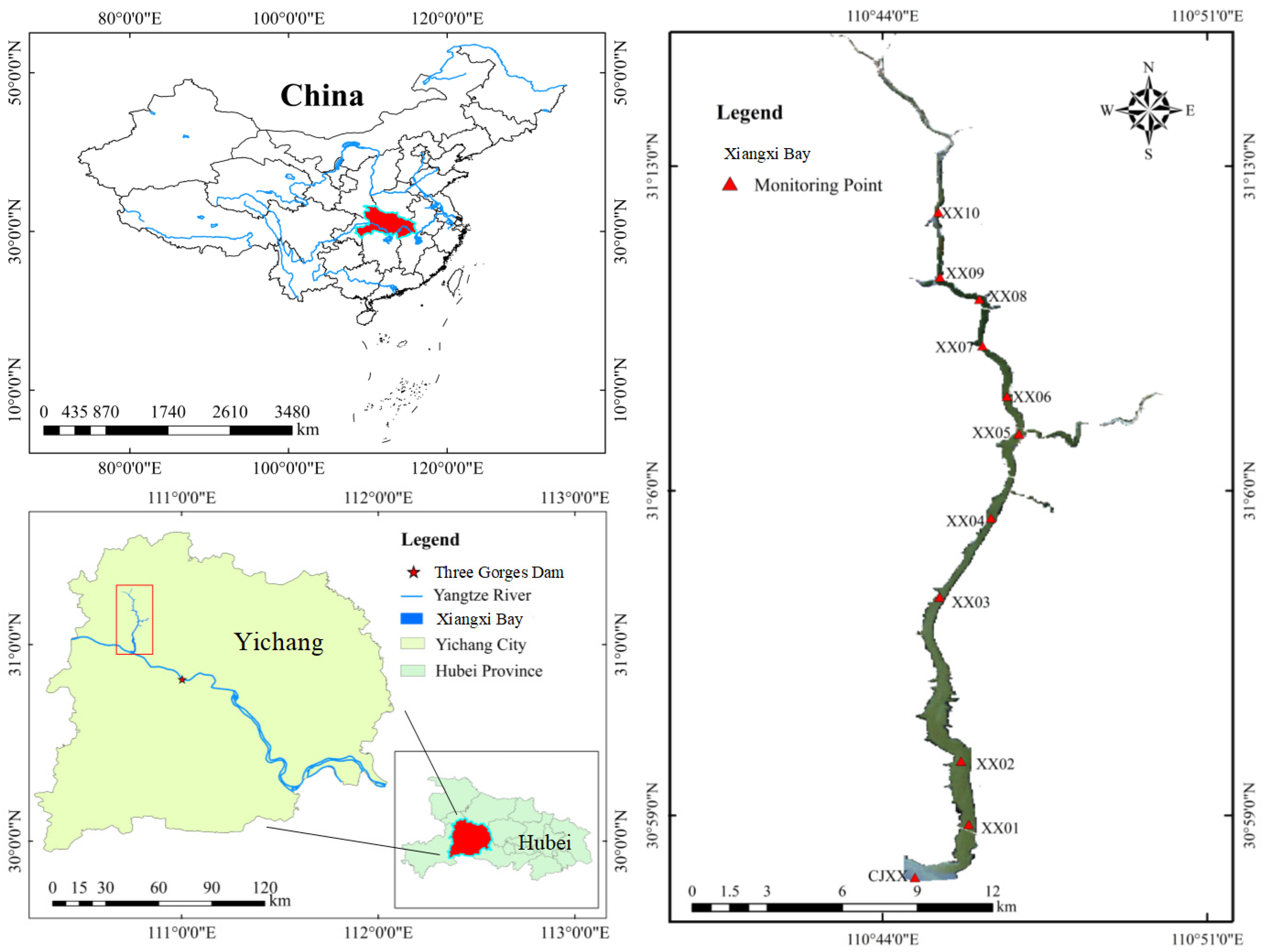
Figure 1. Map of Xiangxi Bay and distribution of monitoring stations.
Remotesensing 17 02886 g001
Figure 2. Workflow of the BP-NN-GSA model, showing four steps: data processing, model training, band fusion, and TSI prediction.
Remotesensing 17 02886 g002
Figure 3. PCA results: (a) variance explained by each principal component; (b) loadings of TSI, TN, TP, WT, WS, SR, PAR, pH, DO and Chl-a on PC1–PC3; (c) biplot of PC1 vs. PC2; (d) sample distribution in PC1–PC2 space.
Remotesensing 17 02886 g003
Figure 4. Heatmap of the correlations between TSI, environmental factors, and water quality nutrient indicators. * indicates Pearson correlation coefficients significant at the 0.05 level (two-tailed), and ** indicates Pearson correlation coefficients significant at the 0.001 level (two-tailed).
Remotesensing 17 02886 g004
Figure 5. Boxplot of TSI values. The values marked in each diamond-shaped box in the figure represent Q1 and Q2.
Remotesensing 17 02886 g005
Figure 6. (a) Original merged spectral curve and (b) spectral curve after outlier removal.
Remotesensing 17 02886 g006
Figure 7. Three-layer BP-NN architecture showing the input layer (WT, SR, PAR, and RS), a hidden layer of optimized neurons, and the TSI output neuron.
Remotesensing 17 02886 g007
Figure 8. Flowchart of the grid search algorithm.
Remotesensing 17 02886 g008
Figure 9. Vertical line plot of R2 values for models with different input combinations: RS; WT + RS; SR + RS; PAR + RS; WT + SR + RS; and WT + PAR + RS.
Remotesensing 17 02886 g009
Figure 10. Comparison of measured vs. BP-NN-estimated TSI values across sample points (R2 = 0.94).
Remotesensing 17 02886 g010
Figure 11. Regression plots of BP-NN outputs versus targets for training (R = 0.96432), validation (R = 0.99172), test (R = 0.99076), and all data combined (R = 0.97151). Training stopped at epoch 15 via early stopping.
Remotesensing 17 02886 g011
Figure 12. Spatiotemporal maps of predicted TSI in Xiangxi Bay in 2009.
Remotesensing 17 02886 g012
Figure 13. Comparison of estimated and measured TSI for 2009.
Remotesensing 17 02886 g013
Figure 14. Predicted TSI distribution in Xiangxi Bay for April and June 2019, and August and November 2020.
Remotesensing 17 02886 g014
Disclaimer/Publisher’s Note: The statements, opinions and data contained in all publications are solely those of the individual author(s) and contributor(s) and not of MDPI and/or the editor(s). MDPI and/or the editor(s) disclaim responsibility for any injury to people or property resulting from any ideas, methods, instructions or products referred to in the content.