Abstract
Hyperspectral image (HSI) denoising is an important preprocessing step for downstream applications. Fully characterizing the spatial-spectral priors of HSI is crucial for denoising tasks. In recent years, denoising methods based on low-rank subspaces have garnered widespread attention. In the low-rank matrix factorization framework, the restoration of HSI can be formulated as a task of recovering two subspace factors. However, hyperspectral images are inherently three-dimensional tensors, and transforming the tensor into a matrix for operations inevitably disrupts the spatial structure of the data. To address this issue and better capture the spatial-spectral priors of HSI, this paper proposes a modeling approach named low-rank Tucker decomposition with subspace implicit neural representation (LRTSINR). This data-driven and model-driven joint modeling mechanism has the following two advantages: (1) Tucker decomposition allows for the characterization of the low-rank properties across multiple dimensions of the HSI, leading to a more accurate representation of spectral priors; (2) Implicit neural representation enables the adaptive and precise characterization of the subspace factor continuity under Tucker decomposition. Extensive experiments demonstrate that our method outperforms a series of competing methods.
1. Introduction
Hyperspectral imaging (HSI) is a sophisticated imaging technique that captures data across hundreds of adjacent spectral bands within the electromagnetic spectrum. These rich spectral-spatial data enable a wide range of applications, including classification [1,2,3,4], super-resolution [5], haze removal [6,7], compressive sensing [8], spectral unmixing [9], and mineral exploration [10]. However, HSI data are often contaminated by noise due to sensor limitations, atmospheric effects, and environmental disturbances [11], which degrades spectral quality and adversely affects downstream tasks. To address this, it is crucial to extract and exploit prior information from the data to enhance denoising performance. Existing HSI denoising methods can generally be categorized into two groups based on their use of prior knowledge: model-based approaches and data-driven methods.
Model-based methods primarily leverage statistical techniques to construct regularization terms that encode prior information in hyperspectral images (HSI). The priors in HSI can be classified into two main types: spectral low-rankness [12,13,14,15,16,17,18] and spatial priors. Spatial priors typically include local smoothness [19,20,21,22,23] and non-local similarity [24,25,26]. However, the effectiveness of model-based methods in utilizing raw data priors tends to be limited [27]. As a result, fast model-based approaches that focus on subspace prior extraction have emerged [28,29,30]. These fast subspace-based algorithms are grounded in the linear mixing model of HSI [31]. According to the unmixing concept, the spectral signature at any spatial point (representing a specific material) can be expressed as a linear combination of the spectral signatures of multiple materials (a set of basis vectors). The spectral signatures of the various materials form the endmember matrix, while the coefficients that represent the abundance of materials at each point in space form the abundance map. If the number of bases in the endmember matrix is chosen to match the rank, the linear mixing model corresponds to low-rank matrix/tensor decomposition. These characteristics of the subspace factors align well with the spatial image structure and spectral continuity of the raw HSI data. Therefore, regularization terms can be directly defined on a smaller-sized subspace matrix to capture the structural priors of the HSI, leading to an acceleration in computation [30]. Existing subspace modeling methods are all based on matrix decomposition. However, the hyperspectral data themselves are three-dimensional cube data. Pulling them into a matrix for modeling will definitely destroy the spatial structure of the data, which is not conducive to the restoration task of high-dimensional images. In addition, both space-based and subspace-based methods face challenges related to insufficient prior characterization. Manually defined regularization terms may fail to capture the unique prior information inherent in the data fully [32].
In contrast, data-driven methods exploit the powerful feature extraction capabilities of neural networks to learn prior information directly from HSI data. Depending on the training approach, these methods can be broadly categorized into three types: supervised learning, plug-and-play, and unsupervised learning. In the supervised learning approach, a deep denoising network is trained using paired clean–noisy HSI data. This method is intuitive and offers fast inference [33,34,35,36,37,38,39]. However, its performance may degrade significantly when the testing data differ from the training data, leading to poor generalization. The plug-and-play approach involves selecting a pre-trained network to function as the denoiser [40,41]. While this method can be effective, it often suffers from structure mismatches and noise level discrepancies between the training domain of the pre-trained model and the target HSI data, leaving room for further improvements. The unsupervised learning approach, on the other hand, directly uses a specially designed network to denoise images with random white noise input, as seen in the Deep Image Prior (DIP) technique [42,43,44,45,46,47]. The core idea is that convolutional neural networks can effectively encode image structure. However, due to the rich spectral and spatial information inherent in HSI data, it is challenging for a single network to fully capture both the spectral and spatial priors in an unsupervised setting. Additionally, determining the optimal early stopping criteria for the network is another challenge, as it is critical to obtain the best possible solution.
To alleviate these problems, we propose a hybrid approach that integrates model-driven and data-driven methodologies. Specifically, we employ low-rank decomposition to capture the spectral correlations inherent in HSI data, while leveraging neural networks to model spatial priors. Unlike previous methods that rely on matrix-based modeling, we directly adopt Tucker decomposition to represent the multi-dimensional low-rank structure of HSI. As illustrated in Figure 1a, Tucker decomposition allows us to constrain the rank along each mode by adjusting the dimensions of the corresponding factor matrices, thereby effectively modeling low-rank characteristics across all three dimensions. The empirical analysis shown in Figure 1c, conducted on the DC mall dataset, reveals significant low-rank properties along all spatial and spectral directions, highlighting the necessity of jointly modeling these dimensions to fully exploit the spectral prior. We further investigate the subspace factor matrices obtained via Tucker decomposition (i.e., Figure 1b), and observe a strong continuity prior, particularly in the spectral mode, as shown in Figure 1d–f. This observation is intuitive—since the factor matrices are derived from the original data, they naturally inherit their spectral continuity and spatial smoothness. This continuity becomes an essential prior that, when accurately modeled, can significantly enhance denoising performance. To capture this continuity, a straightforward approach is to use total variation (TV) regularization. The TV regularization is in the form of differences between adjacent rows and columns, which means that the weight at each point is 1; that is, the continuity of each point is the same, which is inconsistent with the actual situation. As shown in Figure 1d–f, it reveals that the degree of continuity varies across different factors and among the columns within a single factor matrix. This motivates us to go beyond hand-crafted regularization and instead learn the priors adaptively from the data. Inspired by the Deep Image Prior (DIP) [45] and implicit neural representation (INR) [46] techniques, we adopt INR to parametrize each subspace factor to enhance interpretability. Specifically, we employ three fully connected neural networks with sine activation functions to parameterize each factor matrix obtained from the low-rank decomposition. The overall data parameterization process and network architecture are illustrated in Figure 2.
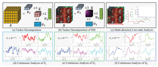
Figure 1.
The spatial and spectral prior analysis for DC mall HSI data. (a) Tucker decomposition diagram—under Tucker decomposition, a third-order tensor can be expressed as the product of a core tensor and three subspace factor matrices , that is, , where is the product between the tensor and matrix; (b) The Tucker decomposition diagram of DC mall data; (c) The multi-way low-rank property of DC mall data, the right subfigures show the singular value curve of the three dimensions; (d) The continuous analysis of each column of the first subspace factor ; (e) The continuous analysis of each column of the first subspace factor ; (f) The continuous analysis of each column of the first subspace factor .
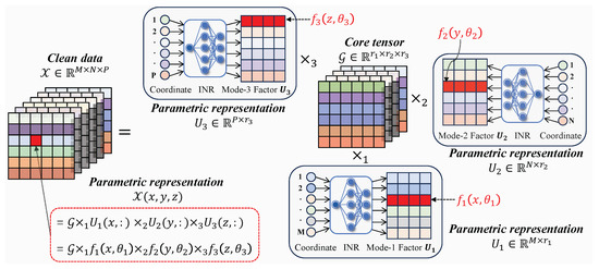
Figure 2.
Schematic diagram of the parametric representation framework for subspace factors under Tucker decomposition. According to the definition of Tucker decomposition, any point on the original data can be represented by the following equation: . Therefore, to capture the spatial information of the original data, it is sufficient to ensure that the columns of each subspace factor exhibit continuity. This continuity can be controlled by a neural network in the framework of neural network parametrization.
In summary, this work makes the following contributions:
- The paper adopts Tucker decomposition to explicitly model the low-rank structure of hyperspectral data across both spatial and spectral dimensions. By decomposing the data into a core tensor and a set of mode-specific factor matrices, this method effectively captures intrinsic correlations along each mode.
- The paper identifies a novel continuity prior in the factor matrices obtained through Tucker decomposition, revealing that the inherent local smoothness and continuity of hyperspectral data are preserved in its subspace representations. This finding provides a new and effective way to characterize the spatial information of HSI data.
- The paper proposes leveraging implicit neural representations to model the continuity of factor matrices. By doing so, each column of a factor matrix can adaptively learn its intrinsic level of continuity, enabling more accurate and flexible encoding of continuity priors.
- The paper develops an unsupervised optimization framework that requires no additional training data. This approach combines the advantages of both model-driven and data-driven methods, eliminating concerns over generalization, and achieves state-of-the-art denoising performance in extensive experiments.
The remainder of this paper is organized as follows. Section 2 reviews related works. Section 3 presents our proposed model and its optimization process. Section 4 presents the experimental results. Finally, the conclusions are drawn in Section 5. Throughout the paper, we denote scalars, vectors, matrices, and tensors in light, bold lower-case, bold upper-case, and upper cursive letters, respectively.
2. Related Work
In this section, we provide a brief overview of the current model-based approaches and several data-driven methods for HSI noise removal.
2.1. Model-Driven Methods
Model-based methods focus on designing regularizers to represent the prior information in HSI data. Common priors include low-rank properties in the spectral dimension, as well as local smoothness and non-local self-similarity in the spatial domain. Low-rank priors assume that HSI data lie in a low-dimensional subspace along the spectral direction, typically modeled using nuclear norms or low-rank matrix/tensor decomposition (LRMD/LRTD) methods like RPCA [13], WNNM [48,49], TRPCA [15,50], HyRes [51], LRMR [14], and NMoG [52]. Local smoothness assumes that neighboring elements in HSI are often similar, and this is usually represented by total variation (TV) regularizers, integrated into low-rank frameworks for better denoising results. Methods like E-3DTV [17], LRTV [19], LRTDTV [20], and CTV [53] apply this regularization. Non-local self-similarity refers to repeating patterns across different spatial areas, and is often incorporated into LRMD/LRTD methods to eliminate noise. Notable methods include KBR [24], BM4D [54], and LLRT [55].
Given the large size of HSIs, applying regularization directly on raw data is inefficient. Subspace-based methods address this by performing low-rank decomposition, allowing for regularizers to be applied to smaller subspace factors. This reduces computation time while preserving important features like local smoothness and non-local self-similarity. Methods such as RCTV [30], NGMeet [29], FastHyDe [26], and LRTFDFR [56] leverage these subspace characteristics for more efficient denoising. Despite their physical interpretability, model-based methods have limitations in fully capturing the unique priors in HSI data, leaving room for improvement in denoising performance.
2.2. Data-Driven Methods
Unlike model-based methods, data-driven methods directly learn a denoising mapping from large datasets. These approaches can be classified into three main categories: supervised learning, plug-and-play, and unsupervised learning. In supervised learning, deep denoising models are trained using paired clean-noisy data, such as in GRN [33], T3SC [38], QRNN3D [34], TRQ3DNet [57], HSID-CNN [35], HSI-DeNet [36], ADRN [58], 3D-ADNet [59], MAC-Net [60], and SST [61]. These methods achieve high fitting accuracy but often face challenges in real-world scenarios due to their limited generalization capability. The plug-and-play method uses a pre-trained network as a denoiser for specific sub-problems within the denoising process. This approach benefits from the robustness of the pre-trained model, resulting in good denoising performance. Representative methods include FastHyMix [40] and AdHyDe [41]. However, since the selected network may not be well matched to the data and noise types, there is still room for improvement. In unsupervised learning, networks are designed to denoise from random white noise inputs without relying on labeled clean data. Examples include DHP [42], DS2DP [43], and S2DIP [46]. While these methods do not require clean labels, they often underperform compared to supervised and plug-and-play methods. For instance, DHP [42] tries to capture spatial and spectral features of HSI, but it struggles to extract sufficient useful information in the unsupervised setting. To improve performance in unsupervised learning, it is crucial to focus on both effective HSI structure modeling and the design of suitable network modules for better prior information extraction.
3. Low-Rank Tucker Subspace Factor Parameterized Representation
3.1. Problem Formulation
Let represent a clean hyperspectral image (HSI), where denotes the spatial dimensions and denotes the number of spectral bands. Assuming the presence of universal additive noise, the observation model can be expressed as:
where represents the observed degraded HSI, captures the Gaussian noise components, and captures the sparse noise, such as impulse noise, stripe noise, data dropouts, and missing pixels [19,20].
Recovering from is a standard inverse problem, and solving such problems necessitates the incorporation of prior knowledge about the data. Generally speaking, the HSI denoising problem can be written as:
where represent the prior term of the clean-image, sparse noise term, and Gaussian noise term, respectively, and denote the trade-off parameters.
3.2. Priori Mining
Common priors for hyperspectral images (HSI) include the low-rank nature of the spectral data and the spatial structural properties of the image. Recalling Figure 1c, we can observe that HSI possesses the low-rankness along all three dimensions. To accurately capture the multi-dimensional low-rank structure of data, a series of tensor decomposition-based methods have emerged [12]. Among them, low-rank Tucker decomposition is one of the most commonly used approaches. The Tucker decomposition is defined as follows:
Definition 1
(Tucker Decomposition [12]). Tucker decomposition factorizes a tensor into a core tensor multiplied by a matrix along each mode. For a 3rd-order tensor , the decomposition is:
where is the core tensor, is the mode product between the tensor and the matrix [12], is the Tucker rank, and are the factor matrices.
According to the definition of Tucker decomposition, if we need to characterize the low rank of multi-dimensional data, we only need to choose a relatively small and appropriate Tucker rank .
Apart from the low-rankness, the local smoothness is another important spatial prior. The local smoothness means that adjacent pixels are likely to belong to the same class of material, and pixels of the same material typically have similar values. Therefore, the total variation (TV) regularization [62] can be used to characterize this property. The definition of total variation is as follows:
Definition 2
(Total Variation [62]). For an image , the total variation regularization is defined as:
where is the difference operator. Or, in the continuous case:
where Ω represents the integration space. For images, Omega is the integration interval in the horizontal and vertical directions.
As seen in Figure 1d–f, each factor matrix exhibits varying degrees of continuity across its columns, which originates from the local smoothness of the image. In fact, HSI can be viewed as a stack of multiple images along the spectral dimension, and these images inherently possess local smoothness;
When an image is further decomposed into a series of vectors, this local smoothness is reflected as continuity among the vectors. A natural approach to modeling vector continuity is to apply TV regularization. However, as shown in Figure 1d–f, the degree of continuity varies across different columns, while TV regularization implicitly assumes uniform weighting at every point of the vector. This uniform assumption fails to capture the varying continuity levels in the factor matrices accurately. Therefore, how to precisely characterize the varying continuity becomes a crucial problem for HSI denoising. Under the low-rank Tucker decomposition, the HSI denoising problem based on the subspace prior mining can be reformulated as:
3.3. Parametric Representation
In model (6), how to mine the prior information of each subspace factor and encode them into is the key to obtaining high-performance denoising performance.
Different from low-rank matrix decomposition, the subspace factor is still an image [28,30,63]. Under Tucker decomposition, the subspace factor is composed of a series of one-dimensional vectors, that is, . Therefore, to characterize the prior of is to characterize the continuity prior presented in Figure 1d–f. From Figure 1, we can observe that there is a significant difference in the continuity between different factor matrices and their respective columns. To better capture the degree of continuity between the columns of different factor matrices, we need to establish a data-adaptive prior representation mechanism. Inspired by the implicit neural representation [64,65], we consider using implicit neural representations to parameterize each factor matrix in the Tucker decomposition. The definition of the implicit neural representation is as follows:
Definition 3
(Implicit Neural Representation [64]). An implicit neural representation is defined as a continuous function parameterized by a neural network with a sine activation function:
where denotes an input coordinate, is the corresponding signal value, and d denotes the dimensions of the input; for example, for a one-dimensional signal and for an image since the image has two dimensions. The function is typically implemented as a multilayer perceptron (MLP) with parameters θ, enabling continuous and differentiable modeling of complex signals.
Based on the definition of INR (i.e., Definition 3), we assign an implicit neural representation network to each factor matrix . Through experiments, we found that a three-layer fully connected network with sine activation functions (using a frequency of 1) yields the best performance. The input to the network is a single scalar, and the number of hidden units is set to four times the height of the data to be reconstructed (e.g., for data of size , the neural number of each hidden layer is set to ). The output is a vector, whose length corresponds to the rank of the respective factor matrix—specifically, the output lengths are , , and for the three-factor matrices . By feeding all coordinate inputs into the network and concatenating the outputs row-by-row, we can obtain the parameterized representation of each factor matrix under Tucker decomposition, as illustrated in Figure 2. Then, we can further obtain the parameterized representation of the needed-to-be-repaired clean data as follows:
where , and are INR network.
For Equation (8), the INR network is implemented as a fully connected neural network with sine activation functions. This architectural choice ensures that the mapping function is inherently continuous and smooth. When the input to the network consists of continuous coordinate values, the output—typically a high-dimensional vector representing image intensity, spectral signature, or other data features—varies continuously with respect to those input coordinates. This guarantees that the INR can preserve continuity in the encoded data along the row-wise (spatial or spectral) direction. More concretely, when coordinate inputs vary smoothly, the corresponding output vectors also change smoothly in each of their dimensions. This continuity ensures that the INR does not introduce artificial discontinuities or artifacts in the encoded representation, which is particularly important for hyperspectral or natural image data, where spatial and spectral coherence are essential. This design ensures that the factor matrices represented by the INR maintain continuity along the row direction. Moreover, as the factor matrices are parameterized by the network, the optimization process enables the network to learn the degree of continuity at each point directly from the data.
3.4. Models
Based on the above analysis, we ultimately adopt Tucker decomposition to model the multi-dimensional correlations of the data to be restored. We use implicit neural representations combined with total variation regularization to capture the continuity of the factor matrices under Tucker decomposition. The Frobenius norm is employed to model Gaussian noise, while the -norm is used to characterize sparse noise. As a result, we formulate the following denoising model:
where , and are coordinate vectors.
From the perspective of effectiveness, both INR and TV regularization are used to characterize the continuity of the factor matrix. However, their effects are different. The TV regularizer assumes that the continuity of the original data between all adjacent rows/columns is consistent, which is obviously inconsistent with the actual situation. Therefore, INR is needed to more finely characterize the continuity of the data. However, model (9) is an unsupervised model, and the parameter update of INR depends on the design of the loss function. In order to enable the network to converge to a better solution, TV regularization is added to Equation (9) to increase the robustness of the model.
3.5. Optimization
Reviewing model (9), it is a constrained optimization problem. Here, we consider directly incorporating the constraint into the optimization objective. Therefore, model (9) can be further expressed as the following optimization model:
For Equation (10), the parameters that need to be updated in the entire optimization objective are the core tensor , Gaussian noise term , and the weights in the network, namely, . We adopt an iterative method to solve the above model (10). In each iteration, the Gaussian noise component and clean data can be updated using the following formula:
where is the soft-threshold operator [53].
For the network parameters and the core tensor , we can directly update them using gradient descent. Giving the learning rate , the update rule is as follows:
For convenience of viewing the entire optimization process and describing more details, we have placed the entire optimization process in Algorithm 1.
| Algorithm 1 LRTSINR for HSI Denoising. |
|
3.6. Time Complexity Analysis
There are two variables that need to be updated in LRTSINR, namely, the Gaussian noise component and clean data . According to the low-rank Tucker decomposition, assuming that the ranks of the clean data in the three directions are , then can be modeled by , where the core tensor has a size of and each factor matrix has a size of . In this paper, a fully connected network with two hidden layers is selected. The number of nodes in the middle layer is , so the number of parameters of each sub-network is . For neural networks, gradient descent is the most commonly used update method. Therefore, in each step of the update, the update parameters required for the three sub-networks are . The number of parameters in is , so the time complexity of updating is . For the Gaussian noise component , it can be solved by the soft threshold operator. For a tensor with size of , the time complexity for updating is . Finally, integrating the time complexity of all variables, the time complexity of Algorithm 1 is .
From the perspective of time complexity, the time complexity of the LRTSINR single step is not high. However, since LRTSINR is an unsupervised method, it should require more iterations to converge to a good result. Therefore, its running time is a little longer. However, with GPU acceleration, the running time of the LRTSINR algorithm is still comparable.
4. Experiments
In this section, we perform extensive experiments on both semi-real noise and real noise data to demonstrate the effectiveness of the proposed model more intuitively.
To evaluate the effectiveness of the proposed model, we compare it against fourteen state-of-the-art (SOTA) methods on both synthetic and real noisy HSI datasets. These competing methods are categorized into two groups: eight model-based methods and six data-driven methods. The model-based approaches include the following: low-rank regularization methods (e.g., LRMR [14]); low-rank combined with total variation regularization (e.g., LRTV [19], LRTDTV [20], CTV [53], RCTV [30]); low-rank combined with non-local self-similarity (e.g., NGMeet [29], GLF [26]); and plug-and-play methods (e.g., FHyMix [40]). The data-driven methods include one unsupervised deep learning method (e.g., S2DIP [46]) and one supervised deep learning method (e.g., RCILD [32]).
To ensure a more comprehensive comparison, we selected two clean datasets for simulated experiments: DC mall and Cloth. The DC mall dataset ( pixels, 160 bands) used in [17] is a synthetic hyperspectral image simulating an urban shopping area, featuring relatively low spatial resolution but rich spectral information in the visible to near-infrared range. This dataset is particularly suitable for evaluating spectral fidelity preservation in denoising algorithms. In contrast, the Cloth (these data are available at https://ieee-dataport.org/documents/cave-hsi#files (accessed on 25 July 2025).) dataset ( pixels, 31 bands) provides high-resolution textile imagery with complex spatial textures but fewer spectral bands, making it ideal for testing spatial detail recovery in denoising tasks. These complementary characteristics allow for comprehensive assessment of denoising algorithms across both spectral and spatial domains. Both datasets serve as clean references for controlled experiments where various noise types can be artificially introduced to simulate real-world scenarios. Furthermore, we select Urban used in [20] and ZY01 used in [66] as the real hyperspectral datasets to evaluate the denoising performance under practical scenarios. The Urban dataset, captured by the AVIRIS sensor over an urban area, has a spatial resolution of pixels and contains 210 spectral bands. It includes diverse ground materials such as rooftops, grass, and roads, making it a challenging dataset due to high spectral variability and noise levels. The ZY01 dataset is acquired from the Chinese ZY-1 satellite and has a spatial resolution of pixels with 166 spectral bands. It primarily captures natural scenes and agricultural regions, and is characterized by severe noise caused by atmospheric and environmental interference. These datasets are widely used benchmarks for evaluating the robustness of denoising algorithms on real noisy data.
All experiments are performed on a PC with an Intel(R) Core(TM) i5-10600KF CPU @ 4.10 GHz, an NVIDIA RTX 3080 GPU, and 10 GB of RAM.
4.1. Synthetic Data Experiments
To comprehensively evaluate the performance of the proposed method, we conduct simulation experiments by comparing it with several competing approaches using both quantitative metrics and visual assessments. The clean hyperspectral image (HSI) dataset DC mall and the multispectral image (MSI) dataset Cloth are used as the ground truth for generating noisy scenarios.
We employ four widely used quantitative metrics to assess image restoration quality as follows: Mean Peak Signal-to-Noise Ratio (MPSNR), Mean Structural Similarity Index (MSSIM), Erreur Relative Globale Adimensionnelle de Synthèse (ERGAS), and Mean Spectral Angle Mapper (MSAM). Then, by adding different degrees of noise (derived from our simulation of real noise), we can calculate the restoration quality by comparing the difference between the denoised data and the original data. Higher MPSNR and MSSIM values, along with lower ERGAS and MSAM scores, indicate better denoising performance. In addition to quantitative evaluation, we qualitatively assess spatial structure preservation and spectral curve recovery to ensure a holistic evaluation.
Since real-world HSI data are often affected by complex noise patterns beyond simple i.i.d. Gaussian noise—including non-i.i.d. Gaussian noise, impulse noise, and deadlines—we simulate five different noise cases as follows:
- (a)
- Each band is corrupted by zero-mean Gaussian noise with a fixed standard deviation of 0.1.
- (b)
- Same as (a), with an additional deadline introduced in DC mall bands 91–130 and Cloth bands 21–30. The width of the deadline is randomly selected from 1, 2, and 3.
- (c)
- Each band is corrupted by Gaussian noise with standard variance 0.075 and salt-and-pepper noise with a missing fraction of 0.15.
- (d)
- Same as (c), with an added deadline in DC mall bands 91–130 and Cloth bands 21–30. The deadline width is randomly chosen from 1, 2, 3.
- (e)
- Each band is corrupted by Gaussian noise with standard deviation randomly sampled from [0, 0.1], and salt-and-pepper noise with missing fraction randomly selected from [0, 0.2]. A deadline is also added in DC mall bands 91–130 and Cloth bands 21–30, with randomly chosen widths from 1, 2, and 3.
Table 1 and Table 2 report the quantitative evaluation results of all competing denoising methods on both hyperspectral (HSI) and multispectral (MSI) datasets across five noise scenarios (cases (a) to (e)). In the LRTSINR model (9), there are three hyper-parameters, namely, . For multi-rank , we use the following settings: , where needs to be fine-tuned and and denote the spatial dimensions (height and width) of the dataset. Since the spectral low rank of hyperspectral images is relatively strong, can generally be selected from 3–15. As for , it controls the continuity of the factor matrix. The smaller the value, the weaker the restriction on smoothness. Therefore, if the texture of an image is complex (that is, there are not so many flat areas), tau should take a relatively small value. In our experiments, we found that for LRTSINR, the tau value range of most remote sensing images is . Therefore, readers can choose the appropriate tau value according to this range and the role of . As for , it controls the ratio between Gaussian noise and sparse noise. If the image contains a lot of Gaussian noise, one can take a smaller beta value to make the Gaussian noise term have a larger value. For the Cloth dataset, the hyperparameter configurations for noise case (a)–(b) and noise case (c)–(e) are , and . Similarly, for the DC mall dataset, the hyperparameter configurations for noise case (a)–(b) and noise case (c)–(e) are and . From these two tables, we can observe the following phenomena. In the simpler settings involving Gaussian noise (cases (a) and (b)), the proposed LRTSINR method does not always outperform state-of-the-art non-local self-similarity (NLSS)-based approaches, such as NGMeet and FHyMix. This outcome is expected, as NLSS-based methods excel at leveraging repetitive patterns across image patches, which aligns well with the spatial properties of Gaussian noise. Therefore, for LRTSINR, a feasible approach is to aggregate similar patches together to form a fourth-order tensor, and then parameterize it using the LRTSINR method, so that LRTSINR can further utilize non-local similarity to improve the Gaussian noise denoising performance. While our method may not achieve the highest MPSNR scores in these specific cases, it still delivers competitive results—consistently surpassing most low-rank and local smoothness-based methods, as well as those requiring supervised training. This highlights LRTSINR as a robust and effective unsupervised alternative even in settings where NLSS techniques dominate.

Table 1.
Quantitative comparison of all competing methods on DC mall dataset. The best and the second best results are highlighted in bold and italic underlined, respectively.
Table 2.
Quantitative comparison of all competing methods on Cloth dataset. The best and the second best results are highlighted in bold and italic underlined, respectively.
However, the performance landscape changes significantly under more complex and realistic noise conditions, such as impulse noise and deadlines—commonly present in practical HSI acquisition scenarios (cases (c) to (e)). In these challenging conditions, NLSS-based methods often struggle to simultaneously remove intricate noise patterns while preserving fine structural details. In contrast, some total variation (TV)-based techniques (e.g., LRTV, LRTDTV, E3DTV, RCTV) exhibit greater resilience to such noise. Most notably, LRTSINR demonstrates clear advantages in these scenarios, achieving the highest MPSNR scores among all competitors and preserving image structure more effectively. Compared to other unsupervised deep learning approaches such as S2DIP, our method shows superior capacity in modeling and mitigating complex noise while maintaining spectral–spatial fidelity.
Furthermore, while supervised learning-based methods offer fast inference and decent denoising quality, they do not achieve top performance in any noise setting. This limitation is likely due to their reliance on specific training data distributions, which may not generalize well to the diverse noise patterns in real-world HSI data. Nonetheless, their efficiency makes them valuable in time-sensitive applications.
We present the pseudo-RGB visualizations of the restored HSI/MSI data under case (e) in Figure 3 and Figure 4 to demonstrate the spatial denoising capabilities of all competing methods. A restoration result is considered superior if it aligns more closely with the ground truth in terms of spatial structure, texture detail, and color fidelity. In each subfigure, an identical subregion is highlighted and magnified four times to facilitate visual comparison. From these visual results, several observations can be made. First, all methods demonstrate the ability to reduce complex mixed noise to some extent. Second, beyond quantitative metrics, our method delivers notable visual advantages. It effectively removes impulse noise artifacts, and deadlines while preserving the original spatial texture and structure of the HSI, exhibiting minimal artifacts and color distortions.
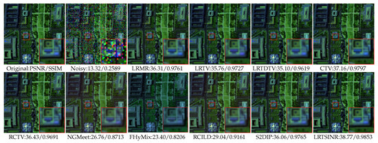
Figure 3.
Recovered false-color images (R: 130, G: 95, B: 14) on the DC mall dataset, with a spatial resolution of , under noise case (e). The corresponding PSNR and SSIM values are shown at the bottom of each subfigure. For better visual comparison, a selected region of interest is enlarged by a factor of four.
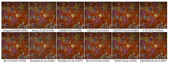
Figure 4.
Recovered false images (R: 30, G: 21, B: 8) on Cloth of the ICVL dataset with a size of under noise case (e). The corresponding PSNR and SSIM values are shown at the bottom of each subfigure. For better visual comparison, a selected region of interest is enlarged by a factor of four.
Additionally, we display the restored spectral signatures at selected locations for all methods in case (e), as shown in Figure 5 and Figure 6. In each spectral subfigure, the ground-truth spectral curve of the clean pixel is plotted alongside the curves recovered by different denoising methods. By comparing these curves, we observe that most methods are capable of effectively suppressing noise while maintaining the overall spectral shape. However, among all the methods, only our proposed approach achieves the closest alignment with the clean spectral curve, clearly demonstrating its superior performance in accurately restoring spectral information.
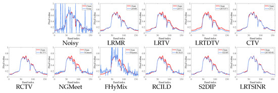
Figure 5.
Recovered spectral curves under noise case (e) of all the competing methods at point (100, 100) on DC mall dataset. There are two curves in each sub-graph, one is the clean spectrum curve, and the other is the spectrum curve restored by denoising methods.
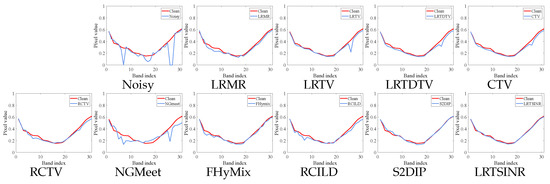
Figure 6.
Recovered spectral curves under noise case (e) of all the competing methods at point (200, 200) on Cloth dataset. There are two curves in each sub-graph, one is the clean spectrum curve, and the other is the spectrum curve restored by denoising methods.
As observed in Table 1 and Table 2, our LRTSINR algorithm does not achieve the highest performance metrics across all cases compared to supervised deep learning. Specifically, it cannot outperform supervised algorithms like RCILD or the plug-and-play method like FHyMix, primarily because these methods leverage pre-trained networks, eliminating the need for inference-time training and often resulting in faster execution. However, when the pre-trained model faces a distribution different from that for its training, its denoising performance drops significantly. This shows that although the supervised method has fast test performance, its results do not have better denoising performance due to generalization issues. Furthermore, our algorithm maintains a relatively fast processing speed when compared to other DIP-based unsupervised methods. A key advantage of LRTSINR becomes evident when contrasted with S2DIP. Our subspace-based modeling significantly reduces the computational burden by decreasing the size of the factors that need to be solved during the optimization process.
4.2. Real Data Experiments
To further verify the adaptability of our proposed method on real noise scenes, we executed denoising experiments on two real-world HSI datasets Urbanpart and ZY01. In addition to the methods used in the simulation experiments, we also introduced the GLF method in real-world experiments, which, like NGMeet and FHyMix, is based on the nonlocal similarity approach. Parts of the spectra of the two HSIs are heavily polluted by atmosphere, water, and some other physical factors, bringing in severe complex noise, including impulse noise, stripe noise, and deadlines. Given the lack of ground truth, it is impractical to quantitatively evaluate all competing methods. Instead, we qualitatively assess the denoising results by showcasing the reconstruction images as pseudo-RGB images of severely affected bands and displaying the spectral curve recovery.
The recovery results for heavily degraded spectral bands are presented in Figure 7 and Figure 8. From these visualizations, it is evident that although all competing methods alleviate real noise to some extent, our proposed approach achieves the most visually appealing results—recovering sharper and more well-defined edge structures. The enlarged subregions further highlight that our method not only effectively suppresses impulse noise and stripe artifacts but also preserves intricate spatial textures, a task that remains challenging for many traditional methods, especially those that do not fully leverage the inherent local smoothness of HSI data.
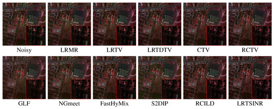
Figure 7.
Recovered false images (R: 132, G: 207, B: 155) on Urbanpart dataset with a size of . For better visual comparison, a selected region of interest is enlarged by a factor of three.
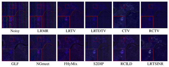
Figure 8.
Recovered false images (R: 165, G: 166, B: 132) on ZY01 dataset with a size of . For better visual comparison, a selected region of interest is enlarged by a factor of three.
In addition to spatial reconstruction, preserving the intrinsic trend of the spectral signature is a crucial criterion for evaluating denoising performance. An effective denoising algorithm should maintain essential spectral priors, such as local continuity, even in the presence of severe noise-induced distortions. As illustrated in Figure 9 and Figure 10, the spectral curves reconstructed by our method exhibit strong local continuity in heavily degraded regions while closely aligning with the reference spectra in relatively clean bands. These results underscore the strength of our approach in maintaining spectral fidelity and demonstrate its robustness against complex, real-world noise.
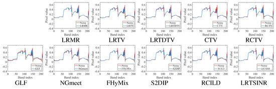
Figure 9.
Recovered spectral curves under noise case (e) of all the competing methods at point (80, 120) on Urbanpart dataset. There are two curves in each sub-graph, one is the noisy spectrum curve, and the other is the spectrum curve restored by denoising methods.
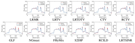
Figure 10.
Recovered spectral curves under noise case (e) of all the competing methods at point (100, 100) on ZY01 dataset. There are two curves in each sub-graph, one is the noisy spectrum curve, and the other is the spectrum curve restored by denoising methods.
5. Conclusions and Future Work
This paper introduces LRTSINR, a unified framework for removing mixed noise from hyperspectral images. Unlike traditional methods that flatten HSI tensors, risking spatial structure disruption, LRTSINR directly operates on the 3D HSI data. It employs Tucker decomposition to model low-rank structures across spatial and spectral dimensions, enabling more accurate spectral prior representation. To capture continuity priors in subspace factor matrices, implicit neural representations adaptively model each factor column’s continuity via coordinate-based neural networks, facilitating precise and data-adaptive spatial prior encoding. Total variation regularization is also incorporated to enhance robustness and spatial smoothness. All parameters are learned unsupervised from observed data without external ground truth.
Extensive experiments on synthetic and real-world datasets demonstrate LRTSINR’s superiority over state-of-the-art methods in both quantitative metrics and visual quality. Future work will explore advanced regularization strategies and neural architectures to improve subspace prior modeling, and extend LRTSINR to broader HSI restoration tasks like inpainting and super-resolution.
Author Contributions
Conceptualization, C.C. and J.P.; Methodology, J.P.; Validation, C.C., D.S., Y.Y. and Z.G.; Formal analysis, D.S.; Investigation, C.C.; Data curation, C.C.; Writing—original draft, C.C.; Writing—review & editing, D.S. and J.P.; Visualization, D.S. and Y.Y.; Supervision, J.P.; Funding acquisition, J.P. All authors have read and agreed to the published version of the manuscript.
Funding
This work was in part by the National Natural Science Foundation of China under Grant 12401674, the Guangdong Basic and Applied Basic Research Foundation under Grant 2025A1515011453, the Fundamental Research Funds for the Central Universities under Grant D5000240095.
Data Availability Statement
The original contributions presented in this study are included in the article. Further inquiries can be directed to the corresponding author.
Conflicts of Interest
The authors declare no conflicts of interest.
References
- Cao, X.; Yao, J.; Xu, Z.; Meng, D. Hyperspectral image classification with convolutional neural network and active learning. IEEE Trans. Geosci. Remote Sens. 2020, 58, 4604–4616. [Google Scholar] [CrossRef]
- Su, Y.; Gao, L.; Jiang, M.; Plaza, A.; Sun, X.; Zhang, B. NSCKL: Normalized spectral clustering with kernel-based learning for semisupervised hyperspectral image classification. IEEE Trans. Cybern. 2022, 53, 6649–6662. [Google Scholar] [CrossRef]
- Jiang, M.; Su, Y.; Gao, L.; Plaza, A.; Zhao, X.L.; Sun, X.; Liu, G. GraphGST: Graph generative structure-aware transformer for hyperspectral image classification. IEEE Trans. Geosci. Remote Sens. 2024, 62, 5504016. [Google Scholar] [CrossRef]
- Su, Y.; Chen, J.; Gao, L.; Plaza, A.; Jiang, M.; Xu, X.; Sun, X.; Li, P. ACGT-Net: Adaptive cuckoo refinement-based graph transfer network for hyperspectral image classification. IEEE Trans. Geosci. Remote Sens. 2023, 61, 5521314. [Google Scholar] [CrossRef]
- Dong, W.; Fu, F.; Shi, G.; Cao, X.; Wu, J.; Li, G.; Li, X. Hyperspectral image super-resolution via non-negative structured sparse representation. IEEE Trans. Image Process. 2016, 25, 2337–2352. [Google Scholar] [CrossRef] [PubMed]
- He, W.; Wang, M.; Chen, Y.; Zhang, H. An Unsupervised Dehazing Network with Hybrid Prior Constraints for Hyperspectral Image. IEEE Trans. Geosci. Remote Sens. 2024, 62, 5514715. [Google Scholar] [CrossRef]
- Zhang, Q.; Yuan, Q.; Li, J.; Li, Z.; Shen, H.; Zhang, L. Thick cloud and cloud shadow removal in multitemporal imagery using progressively spatio-temporal patch group deep learning. ISPRS J. Photogramm. Remote Sens. 2020, 162, 148–160. [Google Scholar] [CrossRef]
- Zhang, L.; Wei, W.; Zhang, Y.; Li, F.; Shen, C.; Shi, Q. Hyperspectral compressive sensing using manifold-structured sparsity prior. In Proceedings of the IEEE International Conference on Computer Vision, Santiago, Chile, 13–16 December 2015; pp. 3550–3558. [Google Scholar]
- Yao, J.; Meng, D.; Zhao, Q.; Cao, W.; Xu, Z. Nonconvex-sparsity and nonlocal-smoothness-based blind hyperspectral unmixing. IEEE Trans. Image Process. 2019, 28, 2991–3006. [Google Scholar] [CrossRef]
- Goetz, A.F. Three decades of hyperspectral remote sensing of the Earth: A personal view. Remote Sens. Environ. 2009, 113, S5–S16. [Google Scholar] [CrossRef]
- Landgrebe, D. Hyperspectral image data analysis. IEEE Signal Process. Mag. 2002, 19, 17–28. [Google Scholar] [CrossRef]
- Kolda, T.G.; Bader, B.W. Tensor decompositions and applications. SIAM Rev. 2009, 51, 455–500. [Google Scholar] [CrossRef]
- Candès, E.J.; Li, X.; Ma, Y.; Wright, J. Robust principal component analysis? J. ACM (JACM) 2011, 58, 1–37. [Google Scholar] [CrossRef]
- Zhang, H.; He, W.; Zhang, L.; Shen, H.; Yuan, Q. Hyperspectral image restoration using low-rank matrix recovery. IEEE Trans. Geosci. Remote Sens. 2013, 52, 4729–4743. [Google Scholar] [CrossRef]
- Lu, C.; Feng, J.; Chen, Y.; Liu, W.; Lin, Z.; Yan, S. Tensor robust principal component analysis with a new tensor nuclear norm. IEEE Trans. Pattern Anal. Mach. Intell. 2019, 42, 925–938. [Google Scholar] [CrossRef]
- Peng, Y.; Meng, D.; Xu, Z.; Gao, C.; Yang, Y.; Zhang, B. Decomposable nonlocal tensor dictionary learning for multispectral image denoising. In Proceedings of the IEEE Conference on Computer Vision and Pattern Recognition, Columbus, OH, USA, 24–27 June 2014; pp. 2949–2956. [Google Scholar]
- Peng, J.; Xie, Q.; Zhao, Q.; Wang, Y.; Yee, L.; Meng, D. Enhanced 3DTV regularization and its applications on HSI denoising and compressed sensing. IEEE Trans. Image Process. 2020, 29, 7889–7903. [Google Scholar] [CrossRef]
- Zhang, H.; Liu, L.; He, W.; Zhang, L. Hyperspectral image denoising with total variation regularization and nonlocal low-rank tensor decomposition. IEEE Trans. Geosci. Remote Sens. 2019, 58, 3071–3084. [Google Scholar] [CrossRef]
- He, W.; Zhang, H.; Zhang, L.; Shen, H. Total-variation-regularized low-rank matrix factorization for hyperspectral image restoration. IEEE Trans. Geosci. Remote Sens. 2015, 54, 178–188. [Google Scholar] [CrossRef]
- Wang, Y.; Peng, J.; Zhao, Q.; Leung, Y.; Zhao, X.L.; Meng, D. Hyperspectral image restoration via total variation regularized low-rank tensor decomposition. IEEE J. Sel. Top. Appl. Earth Obs. Remote Sens. 2017, 11, 1227–1243. [Google Scholar] [CrossRef]
- Xue, J.; Zhao, Y.Q.; Bu, Y.; Liao, W.; Chan, J.C.W.; Philips, W. Spatial-spectral structured sparse low-rank representation for hyperspectral image super-resolution. IEEE Trans. Image Process. 2021, 30, 3084–3097. [Google Scholar] [CrossRef]
- Peng, J.; Wang, H.; Cao, X.; Jia, X.; Zhang, H.; Meng, D. Stable Local-Smooth Principal Component Pursuit. SIAM J. Imaging Sci. 2024, 17, 1182–1205. [Google Scholar] [CrossRef]
- Xue, J.; Zhao, Y.; Wu, T.; Chan, J.C.W. Tensor convolution-like low-rank dictionary for high-dimensional image representation. IEEE Trans. Circuits Syst. Video Technol. 2024, 34, 13257–13270. [Google Scholar] [CrossRef]
- Xie, Q.; Zhao, Q.; Meng, D.; Xu, Z. Kronecker-basis-representation based tensor sparsity and its applications to tensor recovery. IEEE Trans. Pattern Anal. Mach. Intell. 2017, 40, 1888–1902. [Google Scholar] [CrossRef]
- Xue, J.; Zhao, Y.; Liao, W.; Chan, J.C.W. Nonlocal low-rank regularized tensor decomposition for hyperspectral image denoising. IEEE Trans. Geosci. Remote Sens. 2019, 57, 5174–5189. [Google Scholar] [CrossRef]
- Zhuang, L.; Fu, X.; Ng, M.K.; Bioucas-Dias, J.M. Hyperspectral image denoising based on global and nonlocal low-rank factorizations. IEEE Trans. Geosci. Remote Sens. 2021, 59, 10438–10454. [Google Scholar] [CrossRef]
- He, W.; Yao, Q.; Li, C.; Yokoya, N.; Zhao, Q. Non-local meets global: An integrated paradigm for hyperspectral denoising. In Proceedings of the IEEE/CVF Conference on Computer Vision and Pattern Recognition, Long Beach, CA, USA, 15–20 June 2019; pp. 6868–6877. [Google Scholar]
- Zhuang, L.; Bioucas-Dias, J.M. Fast hyperspectral image denoising and inpainting based on low-rank and sparse representations. IEEE J. Sel. Top. Appl. Earth Obs. Remote Sens. 2018, 11, 730–742. [Google Scholar] [CrossRef]
- He, W.; Yao, Q.; Li, C.; Yokoya, N.; Zhao, Q.; Zhang, H.; Zhang, L. Non-local meets global: An iterative paradigm for hyperspectral image restoration. IEEE Trans. Pattern Anal. Mach. Intell. 2020, 44, 2089–2107. [Google Scholar] [CrossRef]
- Peng, J.; Wang, H.; Cao, X.; Liu, X.; Rui, X.; Meng, D. Fast noise removal in hyperspectral images via representative coefficient total variation. IEEE Trans. Geosci. Remote Sens. 2022, 60, 5546017. [Google Scholar] [CrossRef]
- Hong, D.; Yokoya, N.; Chanussot, J.; Zhu, X.X. An augmented linear mixing model to address spectral variability for hyperspectral unmixing. IEEE Trans. Image Process. 2018, 28, 1923–1938. [Google Scholar] [CrossRef]
- Peng, J.; Wang, H.; Cao, X.; Zhao, Q.; Yao, J.; Zhang, H.; Meng, D. Learnable Representative Coefficient Image Denoiser for Hyperspectral Image. IEEE Trans. Geosci. Remote Sens. 2024, 62, 5506516. [Google Scholar] [CrossRef]
- Cao, X.; Fu, X.; Xu, C.; Meng, D. Deep spatial-spectral global reasoning network for hyperspectral image denoising. IEEE Trans. Geosci. Remote Sens. 2021, 60, 5504714. [Google Scholar] [CrossRef]
- Wei, K.; Fu, Y.; Huang, H. 3-D quasi-recurrent neural network for hyperspectral image denoising. IEEE Trans. Neural Netw. Learn. Syst. 2020, 32, 363–375. [Google Scholar] [CrossRef]
- Yuan, Q.; Zhang, Q.; Li, J.; Shen, H.; Zhang, L. Hyperspectral image denoising employing a spatial–spectral deep residual convolutional neural network. IEEE Trans. Geosci. Remote Sens. 2018, 57, 1205–1218. [Google Scholar] [CrossRef]
- Chang, Y.; Yan, L.; Fang, H.; Zhong, S.; Liao, W. HSI-DeNet: Hyperspectral image restoration via convolutional neural network. IEEE Trans. Geosci. Remote Sens. 2018, 57, 667–682. [Google Scholar] [CrossRef]
- Xiong, F.; Zhou, J.; Tao, S.; Lu, J.; Zhou, J.; Qian, Y. SMDS-Net: Model guided spectral-spatial network for hyperspectral image denoising. IEEE Trans. Image Process. 2022, 31, 5469–5483. [Google Scholar] [CrossRef]
- Bodrito, T.; Zouaoui, A.; Chanussot, J.; Mairal, J. A trainable spectral-spatial sparse coding model for hyperspectral image restoration. Adv. Neural Inf. Process. Syst. 2021, 34, 5430–5442. [Google Scholar]
- Zhang, Q.; Zhu, J.; Dong, Y.; Zhao, E.; Song, M.; Yuan, Q. 10-minute forest early wildfire detection: Fusing multi-type and multi-source information via recursive transformer. Neurocomputing 2025, 616, 128963. [Google Scholar] [CrossRef]
- Zhuang, L.; Ng, M.K. FastHyMix: Fast and parameter-free hyperspectral image mixed noise removal. IEEE Trans. Neural Netw. Learn. Syst. 2021, 34, 4702–4716. [Google Scholar] [CrossRef]
- Jiang, T.X.; Zhuang, L.; Huang, T.Z.; Zhao, X.L.; Bioucas-Dias, J.M. Adaptive hyperspectral mixed noise removal. IEEE Trans. Geosci. Remote Sens. 2021, 60, 5511413. [Google Scholar]
- Sidorov, O.; Yngve Hardeberg, J. Deep Hyperspectral Prior: Single-Image Denoising, Inpainting, Super-Resolution. In Proceedings of the IEEE/CVF International Conference on Computer Vision (ICCV) Workshops, Seoul, Republic of Korea, 27 October–2 November 2019. [Google Scholar]
- Miao, Y.C.; Zhao, X.L.; Fu, X.; Wang, J.L.; Zheng, Y.B. Hyperspectral Denoising Using Unsupervised Disentangled Spatiospectral Deep Priors. IEEE Trans. Geosci. Remote Sens. 2022, 60, 5513916. [Google Scholar] [CrossRef]
- Zhang, Q.; Yuan, Q.; Song, M.; Yu, H.; Zhang, L. Cooperated spectral low-rankness prior and deep spatial prior for HSI unsupervised denoising. IEEE Trans. Image Process. 2022, 31, 6356–6368. [Google Scholar] [CrossRef]
- Ulyanov, D.; Vedaldi, A.; Lempitsky, V. Deep image prior. In Proceedings of the IEEE Conference on Computer Vision and Pattern Recognition, Salt Lake, UT, USA, 18–22 June 2018; pp. 9446–9454. [Google Scholar]
- Luo, Y.S.; Zhao, X.L.; Jiang, T.X.; Zheng, Y.B.; Chang, Y. Hyperspectral mixed noise removal via spatial-spectral constrained unsupervised deep image prior. IEEE J. Sel. Top. Appl. Earth Obs. Remote Sens. 2021, 14, 9435–9449. [Google Scholar] [CrossRef]
- Shi, K.; Peng, J.; Gao, J.; Luo, Y.; Xu, S. Hyperspectral Image denoising via Double Subspace Deep Prior. IEEE Trans. Geosci. Remote Sens. 2024, 62, 5531015. [Google Scholar] [CrossRef]
- Gu, S.; Zhang, L.; Zuo, W.; Feng, X. Weighted nuclear norm minimization with application to image denoising. In Proceedings of the IEEE Conference on Computer Vision and Pattern Recognition, Columbus, OH, USA, 23–28 June 2014; pp. 2862–2869. [Google Scholar]
- Gu, S.; Xie, Q.; Meng, D.; Zuo, W.; Feng, X.; Zhang, L. Weighted nuclear norm minimization and its applications to low level vision. Int. J. Comput. Vis. 2017, 121, 183–208. [Google Scholar] [CrossRef]
- Lu, C.; Feng, J.; Chen, Y.; Liu, W.; Lin, Z.; Yan, S. Tensor robust principal component analysis: Exact recovery of corrupted low-rank tensors via convex optimization. In Proceedings of the IEEE Conference on Computer Vision and Pattern Recognition, Las Vegas, NV, USA, 27–30 June 2016; pp. 5249–5257. [Google Scholar]
- Rasti, B.; Ulfarsson, M.O.; Ghamisi, P. Automatic hyperspectral image restoration using sparse and low-rank modeling. IEEE Geosci. Remote Sens. Lett. 2017, 14, 2335–2339. [Google Scholar] [CrossRef]
- Chen, Y.; Cao, X.; Zhao, Q.; Meng, D.; Xu, Z. Denoising hyperspectral image with non-iid noise structure. IEEE Trans. Cybern. 2017, 48, 1054–1066. [Google Scholar] [CrossRef] [PubMed]
- Peng, J.; Wang, Y.; Zhang, H.; Wang, J.; Meng, D. Exact decomposition of joint low rankness and local smoothness plus sparse matrices. IEEE Trans. Pattern Anal. Mach. Intell. 2022, 45, 5766–5781. [Google Scholar] [CrossRef]
- Maggioni, M.; Katkovnik, V.; Egiazarian, K.; Foi, A. Nonlocal transform-domain filter for volumetric data denoising and reconstruction. IEEE Trans. Image Process. 2012, 22, 119–133. [Google Scholar] [CrossRef] [PubMed]
- Chang, Y.; Yan, L.; Zhong, S. Hyper-laplacian regularized unidirectional low-rank tensor recovery for multispectral image denoising. In Proceedings of the IEEE Conference on Computer Vision and Pattern Recognition, Honolulu, HI, USA, 21–26 July 2017; pp. 4260–4268. [Google Scholar]
- Zheng, Y.B.; Huang, T.Z.; Zhao, X.L.; Chen, Y.; He, W. Double-factor-regularized low-rank tensor factorization for mixed noise removal in hyperspectral image. IEEE Trans. Geosci. Remote Sens. 2020, 58, 8450–8464. [Google Scholar] [CrossRef]
- Pang, L.; Gu, W.; Cao, X. TRQ3DNet: A 3D quasi-recurrent and transformer based network for hyperspectral image denoising. Remote Sens. 2022, 14, 4598. [Google Scholar] [CrossRef]
- Zhao, Y.; Zhai, D.; Jiang, J.; Liu, X. ADRN: Attention-based deep residual network for hyperspectral image denoising. In Proceedings of the IEEE International Conference on Acoustics, Speech and Signal Processing, Virtually, 4–8 May 2020; pp. 2668–2672. [Google Scholar]
- Shi, Q.; Tang, X.; Yang, T.; Liu, R.; Zhang, L. Hyperspectral image denoising using a 3-D attention denoising network. IEEE Trans. Geosci. Remote Sens. 2021, 59, 10348–10363. [Google Scholar] [CrossRef]
- Xiong, F.; Zhou, J.; Zhao, Q.; Lu, J.; Qian, Y. MAC-Net: Model-aided nonlocal neural network for hyperspectral image denoising. IEEE Trans. Geosci. Remote Sens. 2021, 60, 5519414. [Google Scholar] [CrossRef]
- Li, M.; Fu, Y.; Zhang, Y. Spatial-spectral transformer for hyperspectral image denoising. In Proceedings of the AAAI Conference on Artificial Intelligence, Washington, DC, USA, 7–14 February 2023; Volume 37, pp. 1368–1376. [Google Scholar]
- Rudin, L.I.; Osher, S.; Fatemi, E. Nonlinear total variation based noise removal algorithms. Phys. D Nonlinear Phenom. 1992, 60, 259–268. [Google Scholar] [CrossRef]
- Wang, H.; Peng, J.; Cao, X.; Wang, J.; Zhao, Q.; Meng, D. Hyperspectral image denoising via nonlocal spectral sparse subspace representation. IEEE J. Sel. Top. Appl. Earth Obs. Remote Sens. 2023, 16, 5189–5203. [Google Scholar] [CrossRef]
- Sitzmann, V.; Martel, J.; Bergman, A.; Lindell, D.; Wetzstein, G. Implicit neural representations with periodic activation functions. Adv. Neural Inf. Process. Syst. 2020, 33, 7462–7473. [Google Scholar]
- Luo, Y.; Zhao, X.; Li, Z.; Ng, M.K.; Meng, D. Low-rank tensor function representation for multi-dimensional data recovery. IEEE Trans. Pattern Anal. Mach. Intell. 2023, 46, 3351–3369. [Google Scholar] [CrossRef] [PubMed]
- Zhang, G.; Ren, R.; Yan, X.; Zhang, H.; Zhu, Y. Effects of microplastics on dissipation of oxytetracycline and its relevant resistance genes in soil without and with Serratia marcescens: Comparison between biodegradable and conventional microplastics. Ecotoxicol. Environ. Saf. 2024, 287, 117235. [Google Scholar] [CrossRef]
Disclaimer/Publisher’s Note: The statements, opinions and data contained in all publications are solely those of the individual author(s) and contributor(s) and not of MDPI and/or the editor(s). MDPI and/or the editor(s) disclaim responsibility for any injury to people or property resulting from any ideas, methods, instructions or products referred to in the content. |
© 2025 by the authors. Licensee MDPI, Basel, Switzerland. This article is an open access article distributed under the terms and conditions of the Creative Commons Attribution (CC BY) license (https://creativecommons.org/licenses/by/4.0/).