Author Contributions
Conceptualization, W.L. and T.J.; methodology, W.L. and S.G.; validation, S.G.; formal analysis, W.L. and Y.Z.; investigation, T.J.; resources, H.W.; writing—original draft preparation, W.L.; writing—review and editing, S.G. and H.W.; visualization, S.G.; supervision, Y.L.; project administration, W.L. and S.G.; funding acquisition, T.J. and S.G. All authors have read and agreed to the published version of the manuscript.
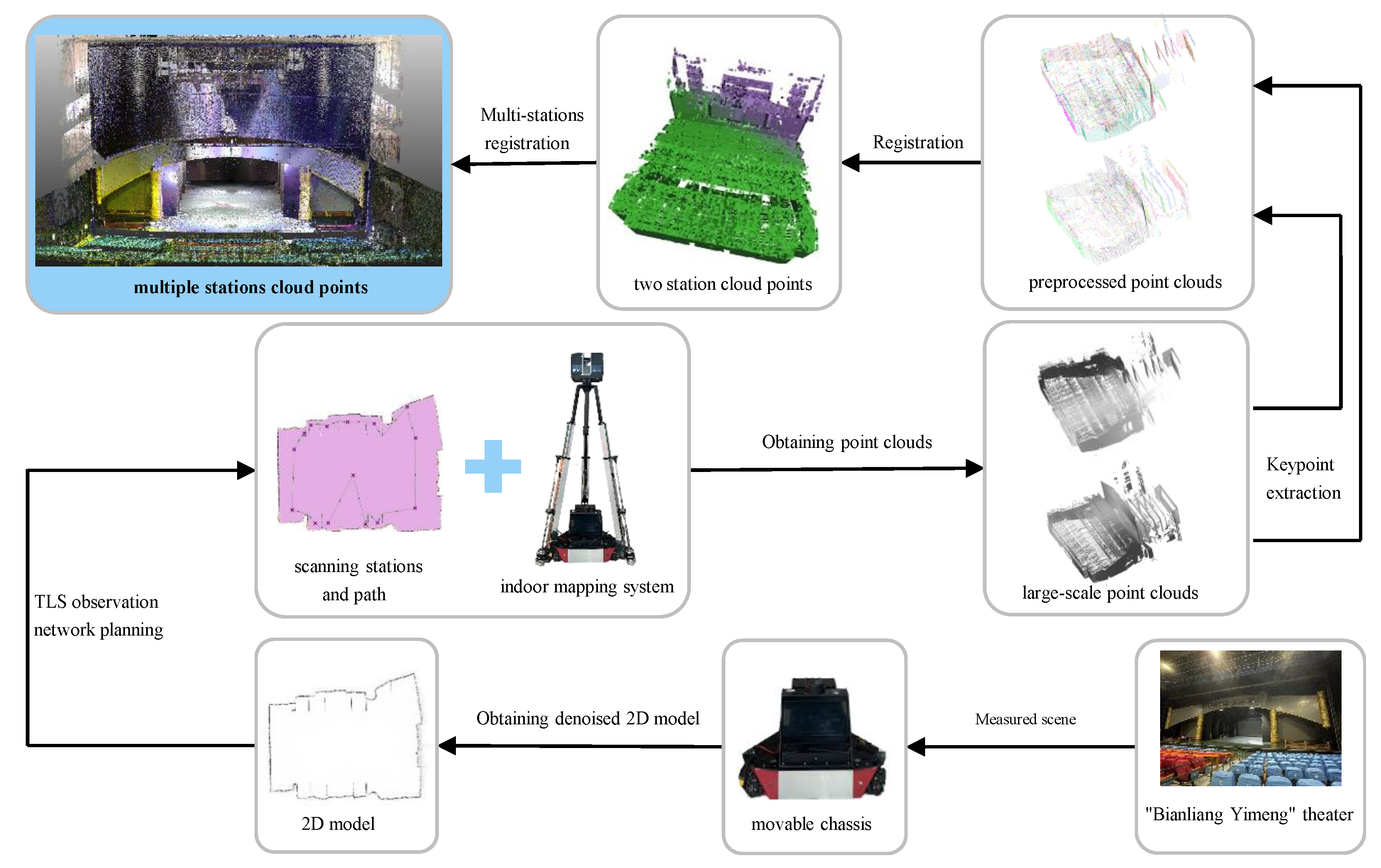
Figure 1.
Overview of the proposed fully automatic indoor surveying framework. The movable chassis collects a 2D model of the theater and performs denoising, using the TLS observation network to determine scan locations and plan paths in unstructured scenes. Keypoints are extracted from the point clouds, which are then aligned using registration algorithms. Finally, creating a complete point cloud model of the “Bianliang Yimeng” theater.
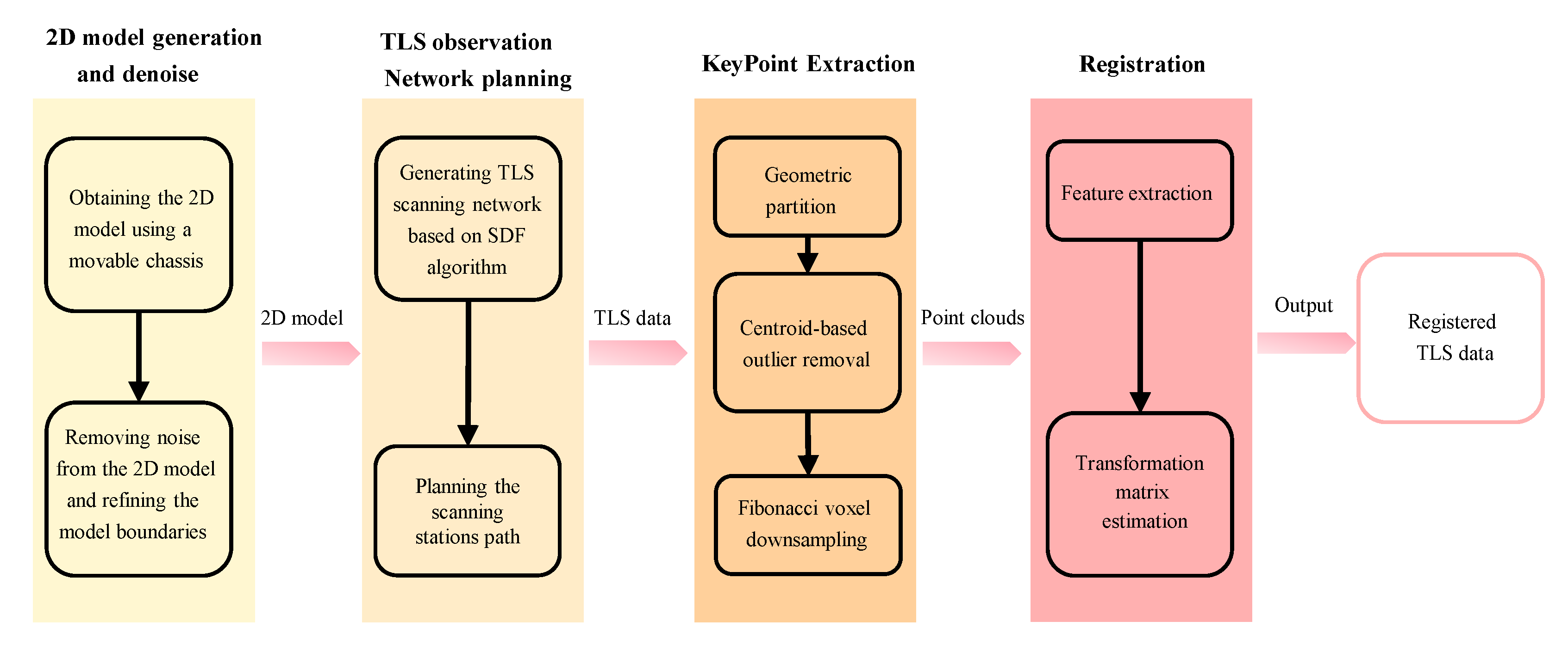
Figure 2.
The flowchart of our method includes four parts: 2D model generation and denoised, TLS observation network planning, keypoint extraction, and registration.
Figure 2.
The flowchart of our method includes four parts: 2D model generation and denoised, TLS observation network planning, keypoint extraction, and registration.
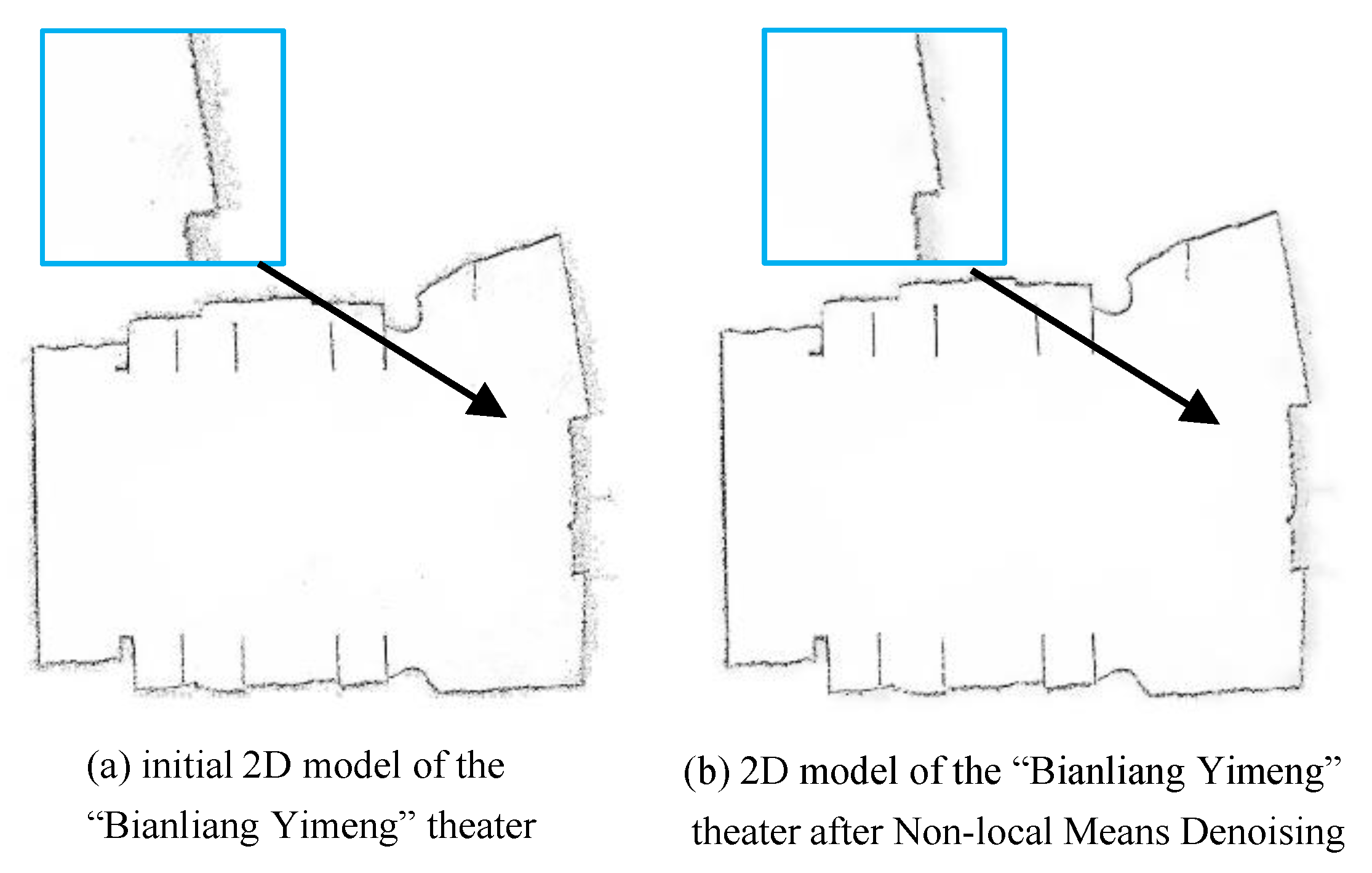
Figure 3.
Comparison of denoised and original 2D model of the “Bianliang Yimeng” theater.
Figure 3.
Comparison of denoised and original 2D model of the “Bianliang Yimeng” theater.
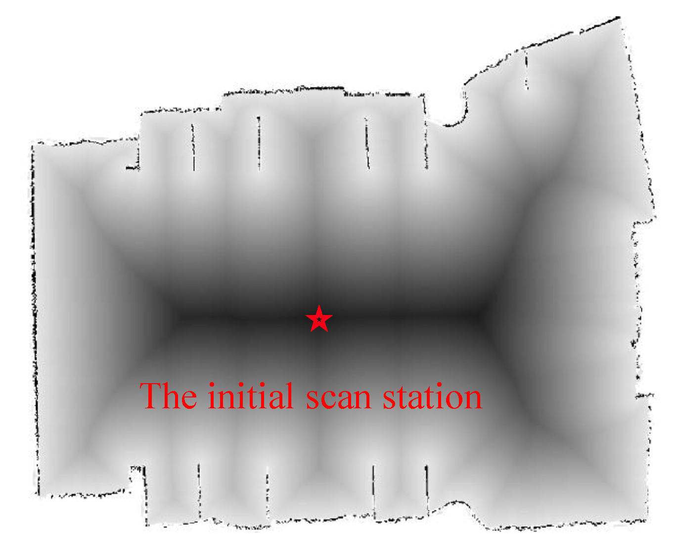
Figure 4.
Initial scan station determined based on the SDF values.
Figure 4.
Initial scan station determined based on the SDF values.
Figure 5.
The locations of the stations obtained after each SDF update, as well as the positions of all stations upon completion of the traversal. The symbol “*” denotes the current station’s position, while the symbol “x” denotes all stations’ positions.
Figure 5.
The locations of the stations obtained after each SDF update, as well as the positions of all stations upon completion of the traversal. The symbol “*” denotes the current station’s position, while the symbol “x” denotes all stations’ positions.
Figure 6.
The relationship between the relaxed point and the obstacle orientation.
Figure 6.
The relationship between the relaxed point and the obstacle orientation.
Figure 7.
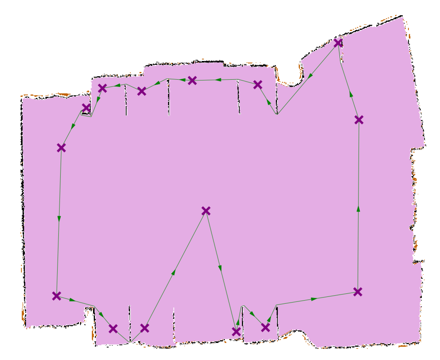
Planning the scan stations’ path. The symbol “x” denotes all stations’ positions.
Figure 7.
Planning the scan stations’ path. The symbol “x” denotes all stations’ positions.
Figure 8.
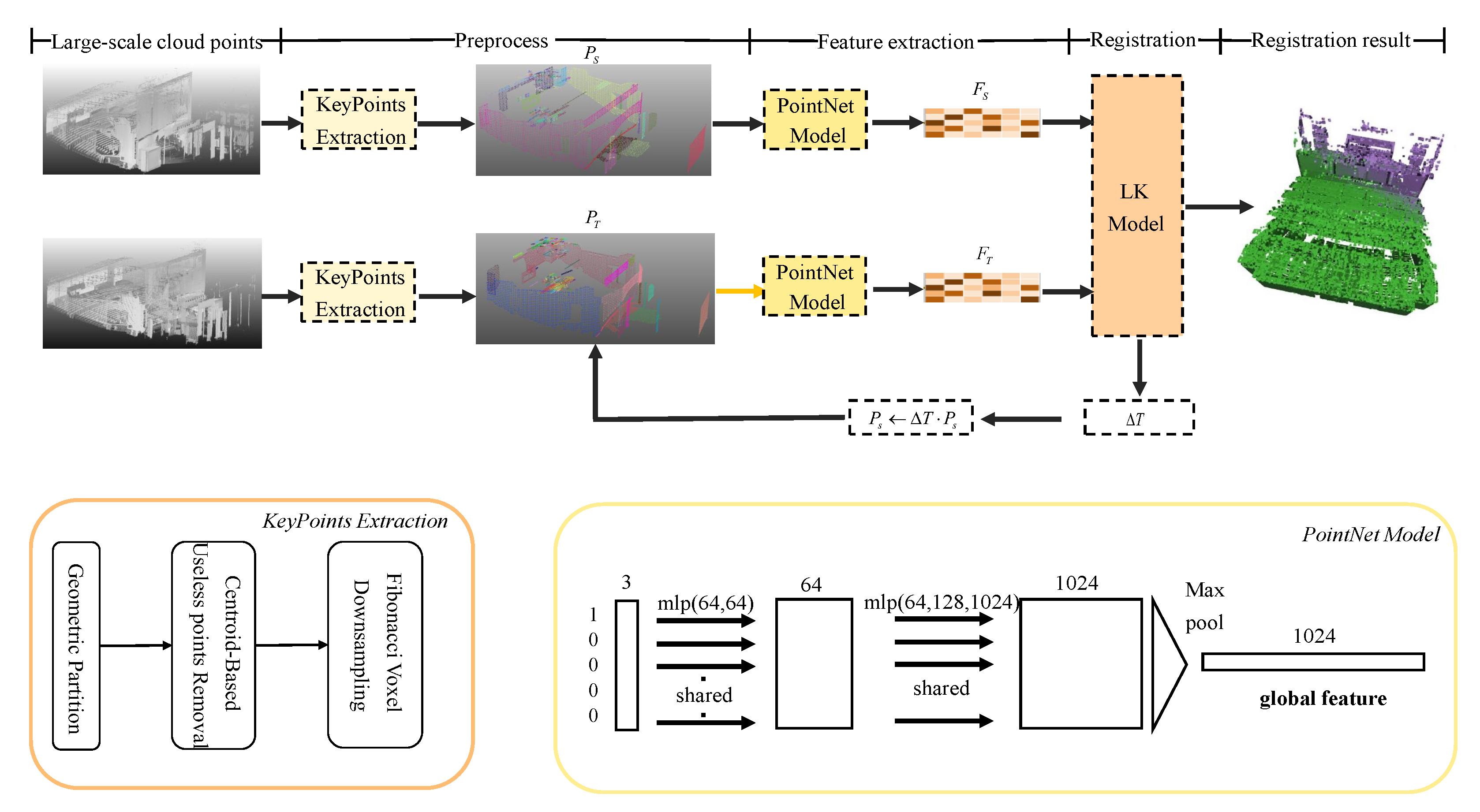
The pipeline of large-scale point cloud registration.
Figure 8.
The pipeline of large-scale point cloud registration.
Figure 9.
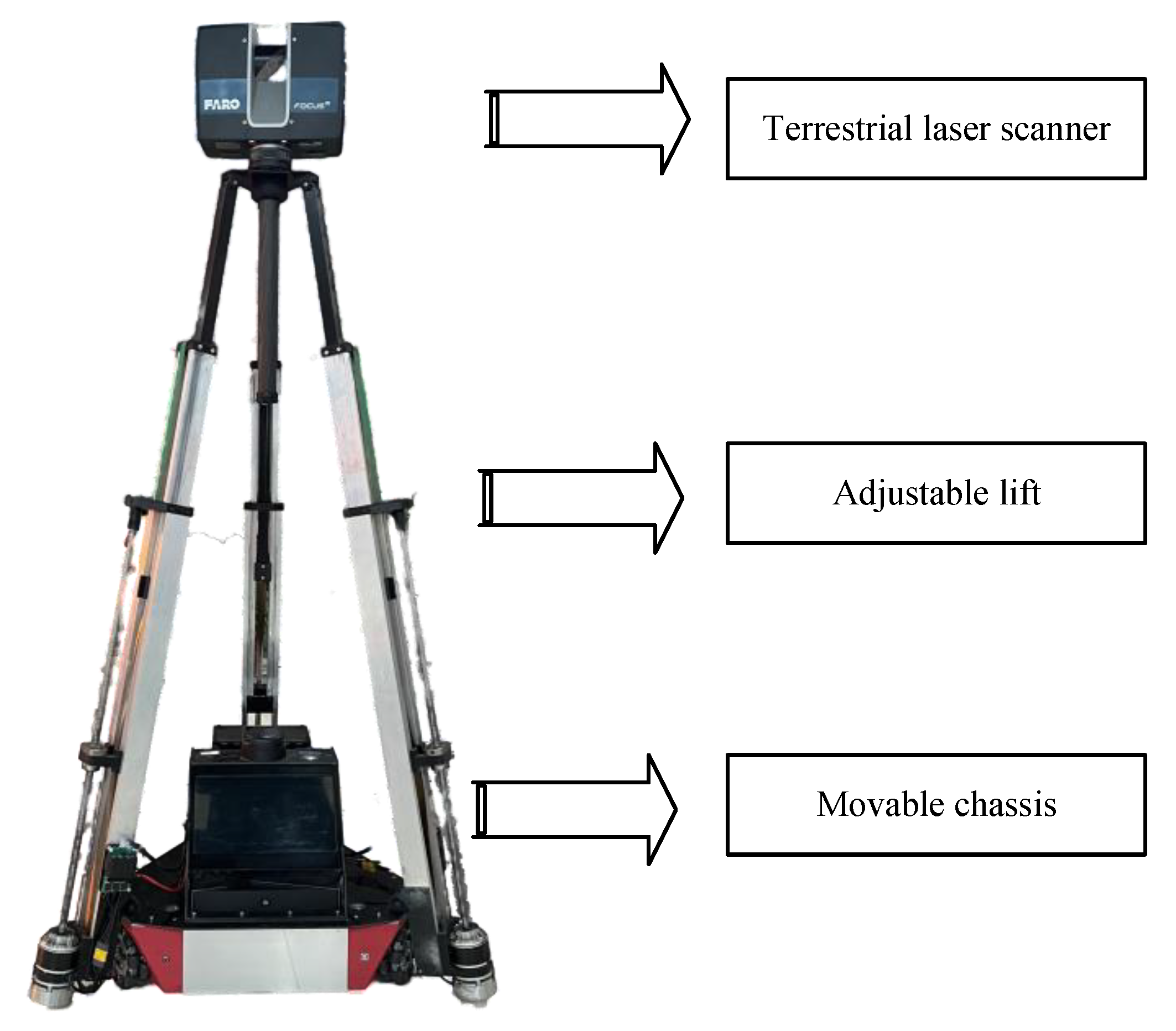
The hardware system physical diagram, viewed from top to bottom, consists of a terrestrial laser scanner, an adjustable lift, and a movable chassis.
Figure 9.
The hardware system physical diagram, viewed from top to bottom, consists of a terrestrial laser scanner, an adjustable lift, and a movable chassis.
Figure 10.
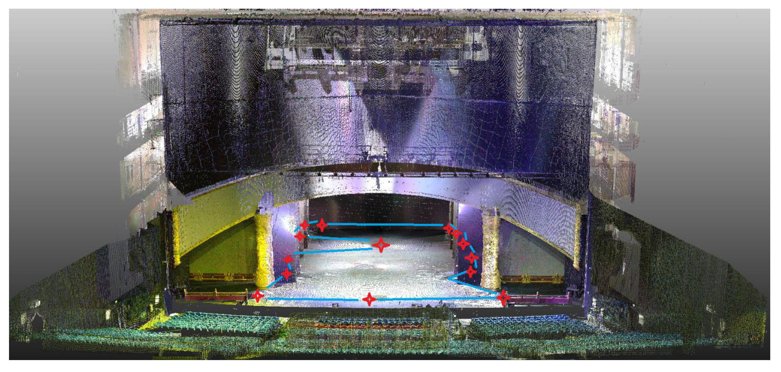
The multi-station point cloud registration results for the “Bianliang Yimeng” theater were obtained through the automatic scanning and marker-free registration system. Blue lines represent the planned station paths and red stars indicate the station locations.
Figure 10.
The multi-station point cloud registration results for the “Bianliang Yimeng” theater were obtained through the automatic scanning and marker-free registration system. Blue lines represent the planned station paths and red stars indicate the station locations.
Figure 11.
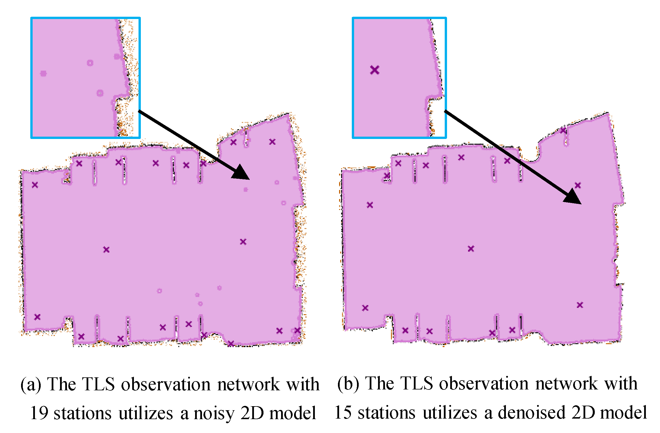
Comparison of denoising effects on the 2D model. The station count was reduced from 19 to 15, demonstrating the effectiveness of our noise suppression approach. The symbol “x” denotes all stations’ positions.
Figure 11.
Comparison of denoising effects on the 2D model. The station count was reduced from 19 to 15, demonstrating the effectiveness of our noise suppression approach. The symbol “x” denotes all stations’ positions.
Figure 12.
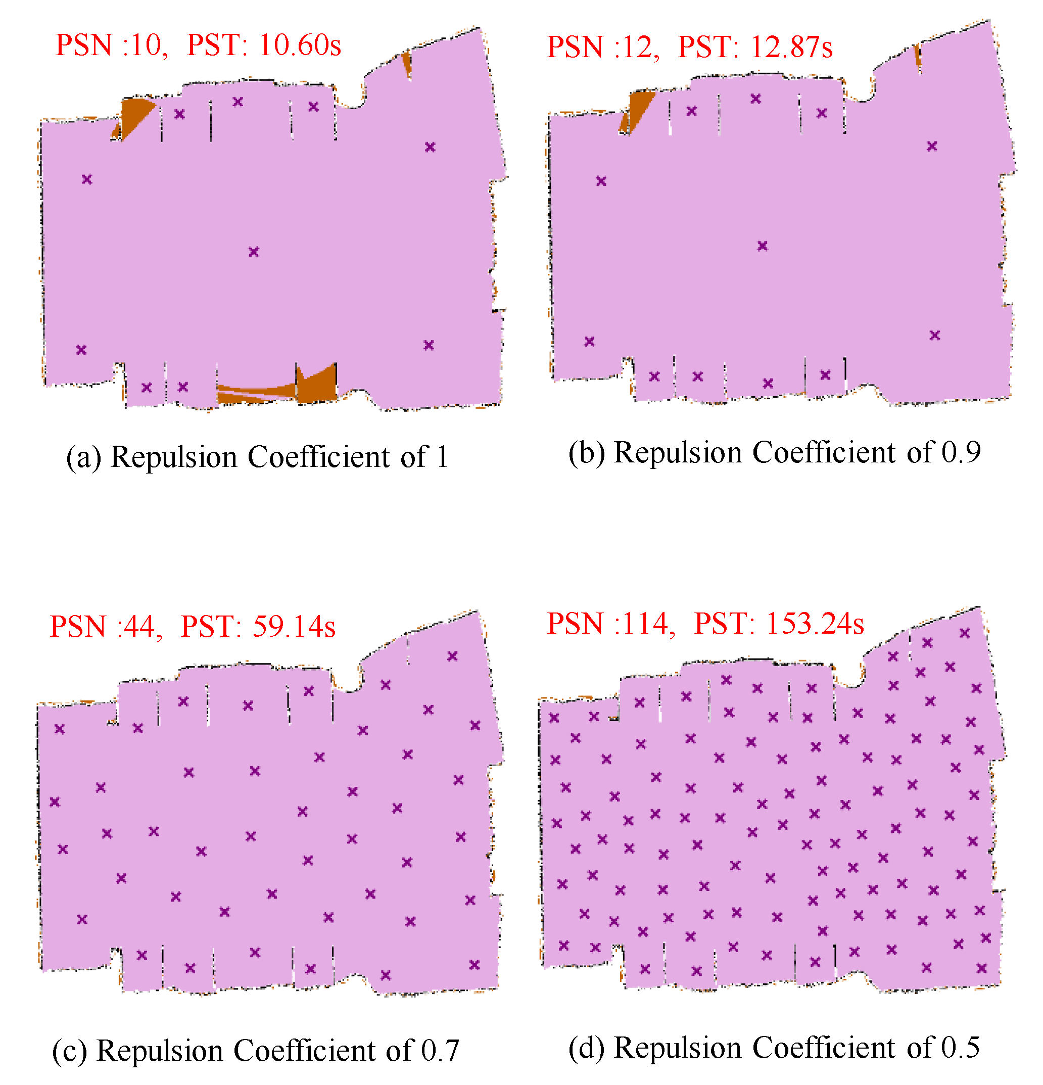
The number of scan stations and scanning time under different repulsion coefficients are shown from (a–d), representing station count and time with repulsion coefficients of 1, 0.9, 0.7, and 0.5, respectively. In the figures, Planning Station Number (PSN) denotes the number of stations, and Planning Station Time (PST) denotes the time. The pink regions denote the scanned areas, while the orange regions denote the unscanned areas.
Figure 13.
When the repulsion coefficient is set to 0.9 and the minimum blind-angle radius is 0.8, the scanning process is able to cover the blind spots effectively. The pink regions denote the scanned areas, while the orange regions denote the unscanned areas.
Figure 13.
When the repulsion coefficient is set to 0.9 and the minimum blind-angle radius is 0.8, the scanning process is able to cover the blind spots effectively. The pink regions denote the scanned areas, while the orange regions denote the unscanned areas.
Figure 14.
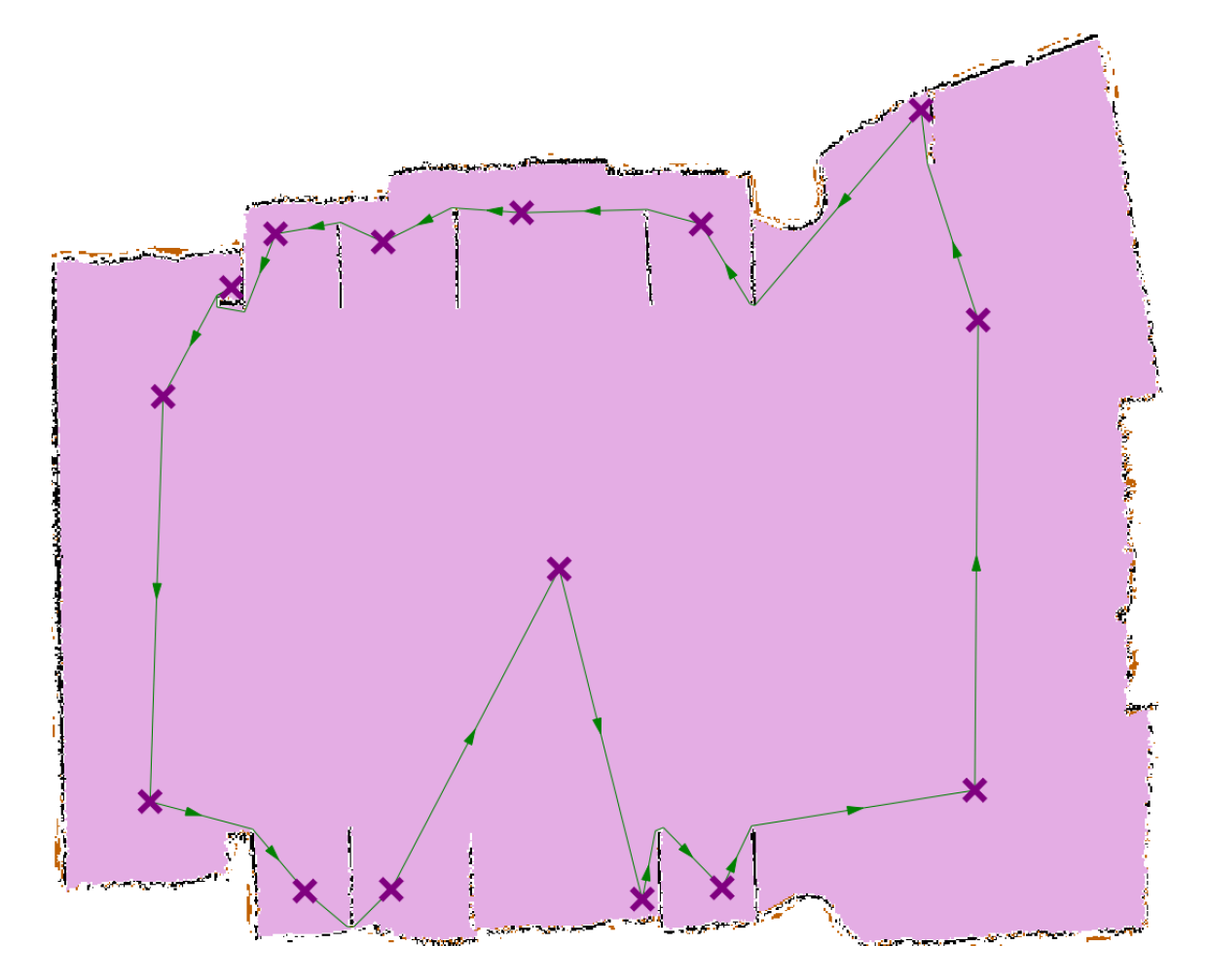
The path planning results for scan stations with a repulsion coefficient of 0.9 and a minimum blind-angle radius of 0.8 are shown.
Figure 14.
The path planning results for scan stations with a repulsion coefficient of 0.9 and a minimum blind-angle radius of 0.8 are shown.
Figure 15.
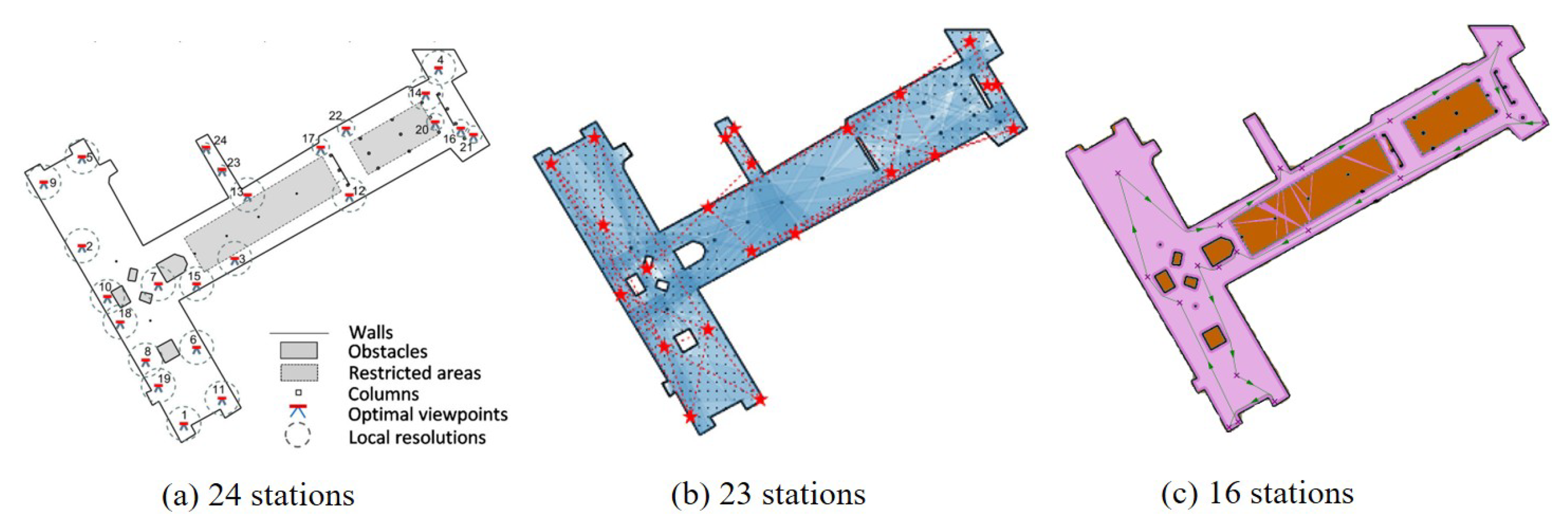
Comparison of the results for the coverage of MacEwan Student Center, University of Calgary using the heuristic method from [
8]: (
a) is the result of [
8] and needs 24 stations; (
b) is the result of [
9] and needs 23 stations; and our method, illustrated in (
c), needs only 16 stations.
Figure 16.
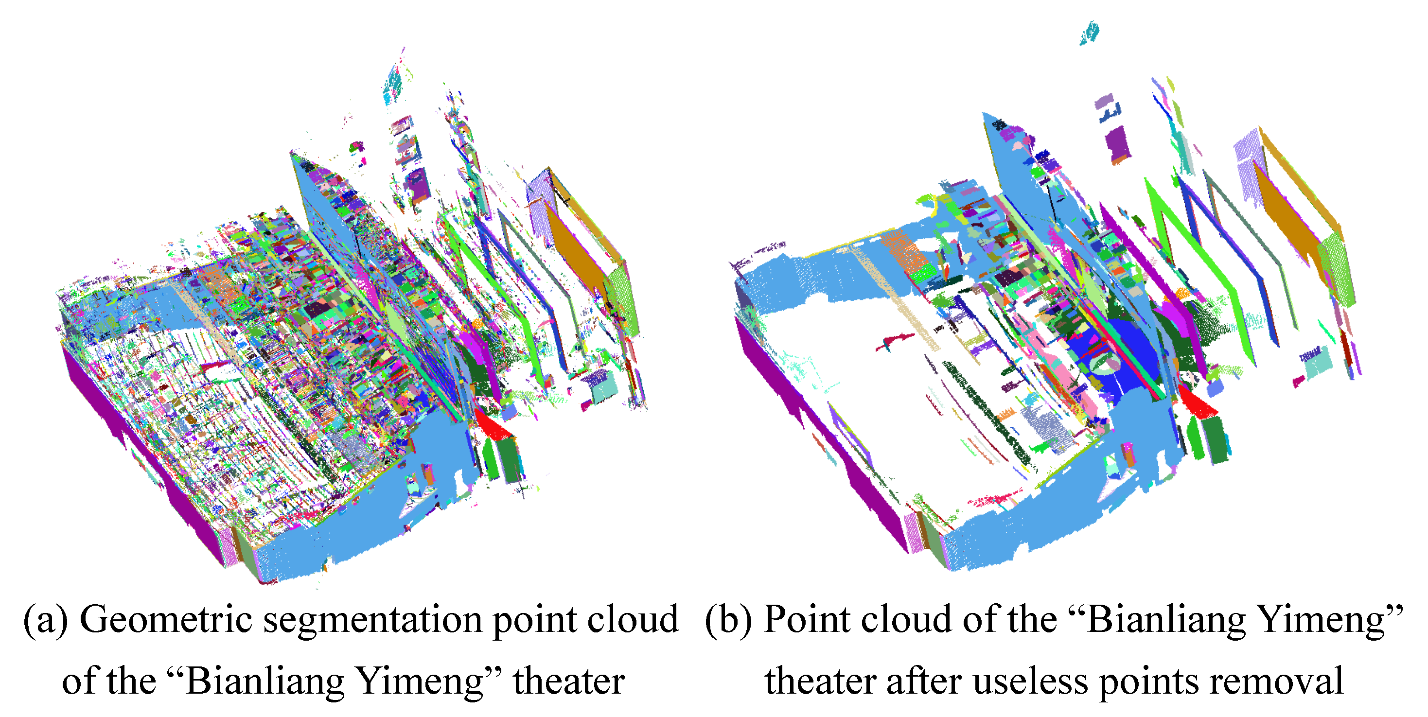
The results of the geometric segmentation. (a) is original point cloud. The colors in (b) are chosen randomly for each element of the partition.
Figure 16.
The results of the geometric segmentation. (a) is original point cloud. The colors in (b) are chosen randomly for each element of the partition.
Figure 17.
The results of the outlier removal. Useless partitions are removed through centroid-based useless points removal method. The colors in (a,b) are chosen randomly for each element of the partition.
Figure 17.
The results of the outlier removal. Useless partitions are removed through centroid-based useless points removal method. The colors in (a,b) are chosen randomly for each element of the partition.
Figure 18.
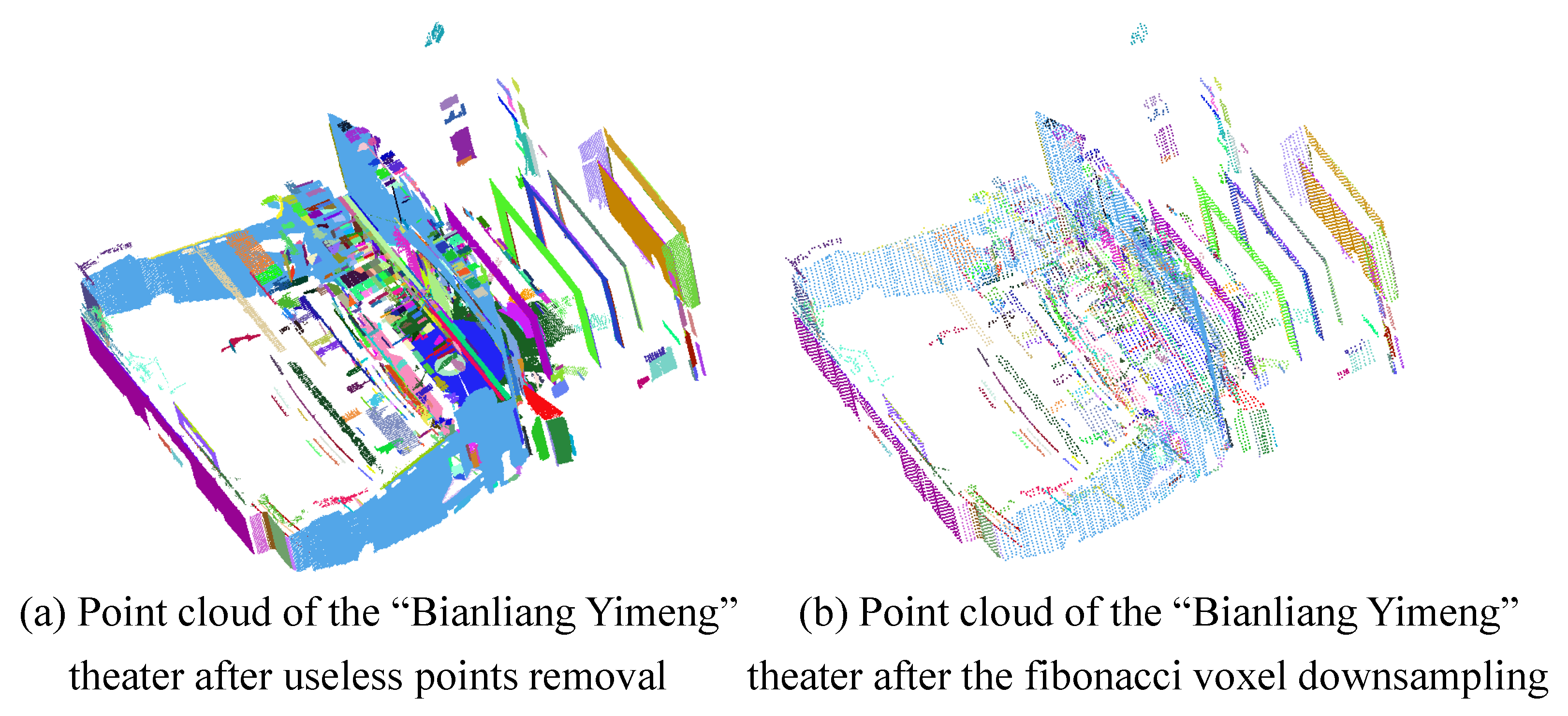
The results of the Fibonacci voxel downsampling. The overall structural information of large-scale scene has been successfully achieved. The colors in (a,b) are chosen randomly for each element of the partition.
Figure 18.
The results of the Fibonacci voxel downsampling. The overall structural information of large-scale scene has been successfully achieved. The colors in (a,b) are chosen randomly for each element of the partition.
Figure 19.
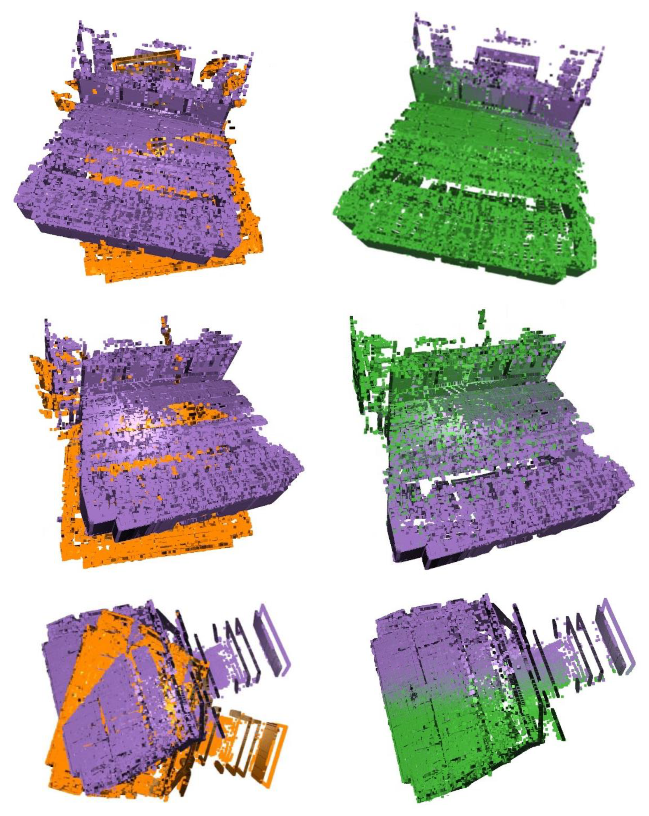
Example visualizations of registration. Color-coded point cloud visualization: Orange represents the source point cloud, purple denotes the target reference cloud, and green indicates the registered point cloud.
Figure 19.
Example visualizations of registration. Color-coded point cloud visualization: Orange represents the source point cloud, purple denotes the target reference cloud, and green indicates the registered point cloud.
Table 1.
In the 2D model of the “Bianliang Yimeng” theater, planning station time and planning path time under different repulsion coefficients are shown.
Table 1.
In the 2D model of the “Bianliang Yimeng” theater, planning station time and planning path time under different repulsion coefficients are shown.
| RC | 1.0 | 0.9 | 0.7 | 0.5 |
|---|
| PST | 10.60 s | 12.87 s | 59.14 s | 153.24 s |
| PPT | 11.09 s | 13.50 s | 63.72 s | 165.10 s |
Table 2.
In the 2D model of the MacEwan Student Center, compare computation time with [
9].
Table 2.
In the 2D model of the MacEwan Student Center, compare computation time with [
9].
| Method | [9] Method | Our Method |
|---|
| Time | 150 s | 34.8 s |
Table 3.
Accuracy comparison with different methods on the 3DMatch dataset. Numbers in bold indicate superior performance.
Table 3.
Accuracy comparison with different methods on the 3DMatch dataset. Numbers in bold indicate superior performance.
| Method | RTE (cm) | RRE (°) | RR (%) |
|---|
| randomDownsample-ICP | 1.078 | 37.877 | 17.2 |
| P2KE-ICP (Ours) | 1.063 | 37.265 | 18.4 |
| randomDownsample-PointNetLK revisited | 1.287 | 47.107 | 2.7 |
| P2KE-PointNetLK revisited (Ours) | 1.183
| 45.862 | 2.8 |
| randomDownsample-REGTR | 0.070 | 2.010 | 78.2 |
| P2KE-REGTR (Ours) | 0.060 | 2.256 | 81.1 |
Table 4.
Registration time results with different methods on the 3DMatch dataset. Numbers in bold indicate superior performance.
Table 4.
Registration time results with different methods on the 3DMatch dataset. Numbers in bold indicate superior performance.
| Method | T (s) |
|---|
| ICP | 35.164 |
| randomDownsample-ICP | 2.2316 |
| P2KE-ICP (Ours) | 1.6303 |
| REGTR | 0.141 |
| randomDownsample-REGTR | 0.0949 |
| P2KE-REGTR (Ours) | 0.0918 |
| PointNetLK revisited | 0.1749 |
| randomDownsample-PointNetLK revisited | 0.1626 |
| P2KE-PointNetLK revisited (Ours) | 0.1663 |
Table 5.
Accuracy comparison with different methods on the Whu-TLS dataset. Numbers in bold indicate superior performance.
Table 5.
Accuracy comparison with different methods on the Whu-TLS dataset. Numbers in bold indicate superior performance.
| Method | RTE (cm) | RRE (°) | RR (%) |
|---|
| sift-REGTR | 0.234 | 64.905 | 20.6 |
| randomDownsample-REGTR | 0.263 | 38.60 | 15.9 |
| P2KE-REGTR (Ours) | 0.250 | 31.695 | 35.3 |
| sift-pointNetLK revisited | 0.13 | 53.22 | 23.5 |
| randomDownsample-pointNetLK revisited | 0.21 | 70.62 | 2.1 |
| P2KE-pointNetLK revisited (Ours) | 0.11 | 38.94 | 31.3 |
