Abstract
Time series of Global Positioning System (GPS) station positions include signals whose characteristics vary over time. Therefore, in detailed analyses, methods dedicated to nonstationary time series should be used. In this study, the Complementary Ensemble Empirical Mode Decomposition (CEEMD) method was used to model trends in time series of GPS station positions and to verify their nonlinearity. As the CEEMD method does not provide equations for assessing the uncertainty of the determined trend, we propose to use the bootstrap method for this purpose. In this study, daily time series of the Up components of 25 GPS stations from seismic regions in Europe and from the Nevada Geodetic Laboratory (NGL) service were used. The determined trends were compared with the trends calculated using the Singular Spectrum Analysis (SSA) method and then interpreted in the context of earthquakes occurring in the vicinity of the station. In turn, the bootstrap method was used to estimate the mean standard deviations of trends determined by the CEEMD as well as SSA method. The conducted studies showed the usefulness of the CEEMD method for modeling trends in time series of GPS station positions, especially for stations where changes may occur on short time scales, visible as the local nonlinearity of the trend, mainly due to earthquake events. The bootstrap-estimated mean standard deviation values for the modeled nonlinear trends are at the level of 1–3 mm, depending on the station. In turn, the root mean square error (RMSE) estimated between the nonlinear trend determined by the CEEMD method and the linear trend fitted to it by the least squares method does not exceed 3 mm. The conducted research indicates that the CEEMD method can be successfully used to model locally nonlinear trends resulting from earthquakes, and the mean standard deviation of the estimated trends is relatively low.
1. Introduction
Global Navigation Satellite System (GNSS) time series hold significant importance in issues related to maintaining and implementing reference systems and are also a valuable source of information for the proper interpretation of geophysical and geodynamic phenomena. Previous studies have shown that changes in GNSS time series are nonstationary and are mainly related to surface mass redistribution in the atmosphere, oceans, and terrestrial water [1], and may also be the result of seismic activity [2,3,4] or long-term changes in surface loading [5]. Thus, GNSS series will contain signals that are variable in time, which is why it is particularly important to use methods dedicated to nonstationary time series studies in their analyses. However, currently the most commonly used methods are deterministic methods of GNSS time series analyses assuming the estimation of linear trends and seasonal components with constant amplitudes and phase-lag. Kermarrec et al. [6] indicate that modeling the unobserved stochastic parts of seasonal trends and signals is important for detecting variability in GNSS time series in connection with their proper geophysical interpretation. Hence, in GNSS time series, both trend and seasonal components should be treated as stochastic processes with deterministic features considered as limiting cases [6].
Determining trends based on time series of GNSS station positions has a wide range of applications, such as determining the long-term stability of a given location or identifying occurring deformations. In this aspect, it is particularly interesting to determine trends for the vertical component. However, GNSS time series with a length of less than 30 years are not always suitable for estimating the long-term linear trend of the vertical component of the crustal movement [7]. Monitoring and studying changes occurring mainly in the vertical movements of the Earth’s crust is largely related to discontinuities as well as changes in trends. Additionally, GNSS time series may contain velocity variables on shorter time scales, which in turn are most often caused by earthquakes and the accompanying post-seismic deformation of the Earth’s crust [8]. Therefore, the nonlinearity of the GNSS station velocity is not obvious, but cannot be excluded, especially in areas of tectonic activity [9]. Additionally, as Hobbs and Ord [10] point out, the consequence of the movement of tectonic plates is the rigid body movements of the Earth’s crust constituting a vector field on the Earth’s surface, while the extent to which the observed trend in the GNSS signal results from the rigid body motion and to what extent from the nonlinear dynamics of the microplate are unknown.
One of the common methods for determining the linear trend in GNSS time series is the Median Interannual Difference Adjusted for Skewness (MIDAS), which is used by the Nevada Geodetic Laboratory (NGL) of the University of Nevada to estimate station velocities and their uncertainties [11]. MIDAS is based on the Theil–Sen median trend estimator, where the site velocity is estimated by the median of the slopes of a large number of selected displacements over a 1-year period. This method is robust to discontinuities, outliers, and seasonality in GNSS time series. However, as the authors of the method point out, this method has limitations, such as the problematic interpretation of the trend in the case of nonlinearity of station velocities, sensitivity to the occurrence of seasonal signals with a frequency other than annual, and lack of robustness of the method to missing data [11]. The second most commonly used method in estimating the linear trend is the Maximum Likelihood Estimation (MLE), which is an iterative minimization process where the inverse of the covariance matrix is calculated at each step [12,13]. In trend analyses based on GNSS time series, it is not only important to model the trend itself, usually in linear form, but also to estimate its uncertainty. In this type of analysis, two approaches to estimating trend uncertainty are distinguished, i.e., the scaling approach and the approach based on noise modeling. In the scaling approach, velocity uncertainty is estimated using one or more scale factors [11,14]. In the approach based on noise modeling, in addition to the parameters of the selected noise model, a linear trend is also estimated, the uncertainty of which in turn is estimated based on the information contained in the covariance matrix [12,13]. The velocity uncertainty thus obtained will depend on the accuracy of the fitted noise models.
Previous studies have shown that if time-varying seasonal signals are not properly modeled, trends in time series and their uncertainties may be incorrectly estimated [15]. Thus, due to the nonstationary nature of GNSS time series, dedicated methods to model time-varying seasonal signals and nonlinear trends are used. In this case, nonparametric methods have been applied, among which the following should be mentioned: wavelet analysis [9,16], singular spectrum analysis (SSA), which allows the decomposition of time series into a number of components, such as trend, periodic components, and noise [17], or Complementary Ensemble Empirical Mode Decomposition (CEEMD) as a method dedicated to the analysis of nonstationary and nonlinear signals [18]. In general, these methods consist of decomposing the analyzed time series into frequency components, which can then be used as models of signals with specific frequencies. In turn, the trends obtained as a result of using wavelet analysis, SSA, or CEEMD do not necessarily have to be linear, which is undoubtedly an advantage of these methods. However, it should be noted that while the SSA and CEEMD methods allow for signal denoising and thus modeling a nonlinear trend, in the wavelet transform, the signal component contains both the signal and the noise in a given frequency range, which should be considered as a certain limitation of this method. At the same time, the main disadvantage of this type of method is the lack of information on the uncertainty of the estimated trend or other periodic signals. Therefore, determining the uncertainty of the estimated trend using time-frequency methods requires the use of additional simulations and statistical methods.
Nevertheless, nonparametric methods have found extended application in analyses related to modeling trends, seasonal signals, and noise in GNSS time series. For example, recently, weighted wavelet analysis was applied to model time-varying seasonal signals in GNSS time series [19], while Kaczmarek and Kontny [20] used wavelet analysis to model GNSS time series to identify the appropriate noise model. In turn, the SSA method was first applied to model seasonal signals in GNSS time series by Chen et al. [17]. Subsequently, the SSA method found application in the analysis of station position time series [21,22] and recently, in an improved form, it was used to directly process incomplete GNSS time series without prior interpolation of missing values [23,24]. Consecutively, the use of the CEEMD method to model seasonal signals in GNSS time series was proposed by Wnęk and Kudas [25]. Moreover, the CEEMD method has also been applied in GNSS time series denoising procedures [26,27]. It should also be mentioned that the earlier form of the CEEMD method, pre-modified EMD, was also used in GNSS time series analyses as a denoising method [28]. Recently, the CEEMD method has also been combined with other methods to increase the efficiency of GNSS time series denoising [29,30,31,32].
Considering the above, it can be noticed that the CEEMD method is successfully used in research related to GNSS time series analysis. However, its application and utilization are focused on denoising GNSS time series or modeling seasonal signals. Therefore, there is a lack of research focusing on modeling trends in GNSS time series, especially nonlinear ones, using the CEEMD method. To fill this gap, the aim of the study is to assess the usefulness of using the CEEMD method to model trends in the time series of Global Positioning System (GPS) station positions and to verify their nonlinearity. Although the CEEMD method enables data mining from noisy time series without prior knowledge of the dynamics affecting the time series and thus allows for obtaining trends that are not necessarily linear, an undeniable disadvantage of the CEEMD method is the lack of a quantitative assessment of the analysis performed. Since it is very important to estimate the uncertainty of GNSS time series trends, in this study, we propose to combine the CEEMD trend estimation with the bootstrap method to assess their uncertainty. The bootstrap method allows for the determination of estimation errors using multiple sampling with replacement from the sample. For this purpose, 200 simulations were performed for each station, which then allowed for determining the average standard deviation. The nonlinear trends determined using the CEEMD method were interpreted in relation to earthquakes noted near particular stations. Additionally, the obtained trends were compared with nonlinear trends modeled using the SSA method, for which uncertainties were also estimated using the bootstrap method. Only the Up component (U) of the GPS time series of selected stations made available in the NGL service from seismic regions in Europe was used in the analyses. Since the time series provided by NGL process only GPS observation, we will use the GPS nomenclature instead of GNSS in the rest of this article.
The remaining parts of this paper are organized as follows. Section 2 describes the data used and justifies the selection stations for analysis. This section also presents the CEEMD decomposition method as well as the bootstrap method. Section 3 presents the results of the analyses, estimating nonlinear trends using the CEEMD decomposition and assessing their mean standard deviations using the bootstrap method. Section 4 discusses the obtained results in the contest of the current state of knowledge regarding the geophysical interpretation of nonlinear trends in GPS time series, and identifies the advantages and disadvantages of the CEEMD method, as well as future research directions. Section 5 summarizes the most important conclusions from the conducted research.
2. Materials and Methods
2.1. Data
The study used selected daily time series of U components of GPS station positions from the NGL service [33] and expressed in an IGS14 frame. The time series of station positions provided by NGL are processed in the Precise Point Positioning (PPP) mode. Detailed information on the data analysis strategy and NGL products can be found at: http://geodesy.unr.edu/gps/ngl.acn.txt (accessed on 20 April 2025).
Selected stations are located in Europe, particularly in its southern part (Figure 1), in areas characterized by seismic activity [34]. According to data contained in the U.S. Geological Survey (USGS) Earthquake Catalog [35], over 18,000 earthquakes with magnitudes above 2.5 were recorded in the considered region and its surroundings in the period 2006–2024. At the same time, only about 2% of the earthquakes had a magnitude above 5. The region is dominated by earthquakes with magnitudes between 3 and 4. The earthquakes usually occur here at a depth of up to 100 m (approximately 97% of the presented earthquakes). Furthermore, stations such as PAT0, NOA1, IZMI, and TUC2 are located on the Aegean microplate. NOT1 is located on the African tectonic plate, while NICO is located on the Anatolian microplate. The remaining stations are located on the Eurasian plate, with TUBI located on the boundary of the Eurasian and Anatolian plates. From the quite large set of stations’ position data, those that were additionally classified as stations belonging to the European EUREF Permanent Network (EPN) were selected, due to their geodetic quality resulting from additional standards for the foundation and equipment of stations defined by EPN. However, the analyses did not use the network solutions of station positions from EPN. Finally, 25 stations were selected for analysis, which are characterized by a data length of at least 8 years and data completeness above 94%. The average length of missing data is 3%. Due to the long data gaps, some time series were shortened at the beginning or at the end, hence accounting for the different start and end dates (Table 1). The length of the analyzed time series ranges from 8.3 years to 27.3 years.
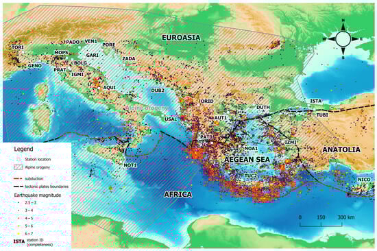
Figure 1.
Location of the stations with the presentation of the digital model of plate boundaries based on [35,36] and earthquake center location (own study using GEBCO_2022 Grid color-shaded for elevation available at https://wms.gebco.net/2022/mapserv, accessed on 9 July 2025).

Table 1.
Length of time series used in the analysis, including start and end dates, data completeness, and longest period of missing data.
The time series of station positions were preprocessed before analysis by identifying data discontinuities and removing outliers. The noted discontinuities caused by equipment changes at the stations or those resulting from earthquakes were manually identified [37,38], individually for each station based on information from the NGL service [39]. Outliers are defined as elements more than three scaled Median Absolute Deviation (MAD) from the median, and outliers were replaced by linear interpolation of neighboring nonoutlier values. Since the use of time series analysis methods most often requires continuous data, missing data were interpolated using autoregressive modeling. As shown in the work of Wnęk and Kudas [25], interpolation for 5% of missing data does not have a significant impact on the obtained results using the CEEMD method. In the interpretation of the results for selected stations, information on the occurring discontinuities related to equipment replacement and earthquakes [39] was used.
2.2. Complementary Ensemble Empirical Mode Decomposition
To determine trends in selected time series of the vertical position of the station, decomposition using the CEEMD method was used, which is an adaptive time-frequency method dedicated to the analysis of nonlinear and nonstationary time series. The CEEMD method was proposed by Yeh et al. [18], and is a modification of the original Empirical Mode Decomposition (EMD) method [40,41,42] by eliminating the problem of mode mixing as well as the problem of residual noise in the reconstructed signal. In the CEEMD method, the signal is adaptively decomposed into a finite number of intrinsic mode functions (IMFs), which are a family of classes of functions based on local properties of the original signal. Thus, the IMFs are complete and almost orthogonal and represent the signal divided into frequency components ordered from the highest to the lowest frequencies.
Any time series , where , and is the length of the time series, can be decomposed using the CEEMD method as follows:
- Generating a pair of signals by adding and subtracting white noise ε(t) from the original time series
- Separate decomposition of signals and using the EMD method as follows:
- (a)
- Identification of extrema at and ;
- (b)
- Determination of upper and lower envelope, by separately connecting all local minima and maxima using cubic spline line;
- (c)
- Determination of envelope mean and and first components and as follows:and then verifying whether and meet the condition for IMF. If the condition is met, then and , otherwise the procedure is repeated —times until the condition is met, and during the repetition, the next and are considered accordingly in the following way
- (d)
- Separation of the first component from the datawhere and will be considered as new datums, for which the procedure at points a–d will be repeated times, until is so small that no more local extrema and can be extracted, or until and become monotonic functions.
The entire decomposition procedure is repeated times, and in the case of this study, the value of is assumed to be 100. Thus, CEEMD creates two sets of with added noise and with removed noise, which are then averaged to obtain the final set of representing the distribution of the time series , as follows:
where may be an average trend or constant.
More information on EMD and its modifications can be found in publications such as Huang et al. [40], Wu and Huang [43], and Yeh et al. [18]. The application and usefulness of the CEEMD method for the decomposition of time series of GNSS station positions was verified and presented in Wnęk and Kudas [25,32].
2.3. Bootstrap
The CEEMD method has an obvious disadvantage, namely the lack of uncertainty estimation for individual IMFs as well as residuals that are the average trend. Therefore, in order to estimate uncertainty, additional statistical methods must be used. In this study, the bootstrap method was used to estimate the uncertainty of residuals, i.e., the obtained trend. Bootstrap is a statistical tool that allows for the quantitative determination of uncertainty associated with a given estimator or statistical learning method, where it is difficult to obtain a measure of variability and confidence intervals are directly determined based on real data [44,45]. This method consists of randomly selecting samples with replacement from a data set and then analyzing each sample in the same way. Sampling with replacement means that each observation is selected separately at random from the original data set, and each element of the original data set may appear many times in a given sample. The number of elements in each bootstrap sample is equal to the number of elements in the original data set, and the range of sample estimates obtained allows the uncertainty in the estimated quantity to be determined.
The bootstrap method was used to assess the uncertainties of determining trends using the CEEMD method in the GPS time series under consideration. For this purpose, residuals were determined, here created by subtracting the IMFs representing seasonal signals, i.e., semi-annual and annual (IMF5 and IMF6) [25], and the trend from the sum of IMFs. Random sampling with replacement was performed 200 times in each case, and then the average standard deviation for a given time series was determined, which can be interpreted as the uncertainty of the trend estimated using the CEEMD method. In other words, this approach allowed for the assessment of how the trend determined using the CEEMD method will behave when samples are repeatedly taken from a modified time series not containing semi-annual and annual signals and the estimated trend. In this case, it was decided to exclude the dominant seasonal signals, given that their occurrence has been proven in numerous studies and is currently taken into account in International Terrestrial Reference Frame (ITRF) implementations [46,47].
Additionally, a comparative analysis was also performed, comparing the nonlinear trends estimated using the CEEMD method with the nonlinear trends computed using the SSA method. The SSA method decomposes the time series into independent components, such as trend, periodic components, and noise. The decomposed time series is embedded in a trajectory matrix by shifting a window of appropriate size, and then a covariance matrix is constructed. In this study, a 3-year window was used, and the presence of seasonal signals, i.e., annual and semi-annual, was assumed. The bootstrap method was also used to estimate the uncertainty of the trends determined using the SSA method, using the same principles as for estimating uncertainty in the CEEMD method. Details regarding the SSA method can be found in Chen et al. [17].
All calculations were performed using MATLAB R2023b [48].
3. Results
In the CEEMD method, the signal is divided into a finite number of IMFs, which represent instantaneous frequencies as a function of time. The IMFs obtained in the decomposition process are ordered from the highest to the lowest frequency, and each IMF is more general than a simple harmonic function due to time-dependent amplitudes and frequencies. Therefore, first, the CEEMD decomposition of the station position time series was performed.
At this point, it is also necessary to mention the discontinuities occurring in the GPS time series, which result from the following events: a change in station equipment or an earthquake. The former is identified by a recorded change in station equipment or by a fault causing noticeable changes in the station’s position time series. Discontinuities resulting from earthquakes, on the other hand, can occur when the earthquake is large enough and the distance from the epicenter close enough to expect a displacement of more than 1 mm [49]. In turn, failure to take into account phenomena related to tectonic activity in the analyses of time series of station positions has a significant impact on the estimated linear motion and increases its uncertainty [50]. Taking this into account in this study, the noted discontinuities caused by equipment changes at the stations or those resulting from earthquakes were manually identified [28,37], individually for each station based on information from the NGL service [39]. In the case when the time series showed an identified shift of the U component, e.g., stations BOLG, PRAT, or TORI, trends were determined separately for specific time intervals. Also, what was not always noted at the station events, such as equipment changes or earthquakes, caused significant steps in the time series, i.e., breaks are too small to be detected in a noisy signal. In turn, GPS time series may also contain discontinuities not recorded in log files, the nature of which is unknown and may be the result of unnoted human activities or natural phenomena [51]. Moreover, in some cases, the separated time intervals between adjacent breaks may be too short to allow for reliable modeling of the trend and periodic components, e.g., in the case of the TORI station.
Figure 2 shows the modeled seasonal, semi-annual, and annual signals and the CEEMD trend for the U component, for example, for the time series of stations where no significant discontinuities due to seismic activity or equipment changes were detected. The seasonal signals modeled using the CEEMD method are clearly characterized by variability in time, which has already been shown by Wnęk and Kudas [25,32], while in the case of trends, their local nonlinear character can also be observed. If no earthquake event occurred in the vicinity of the station, then the trends are usually close to linear, e.g., stations: AQUI, GENO, ISTA. In some cases, the determined trend is locally nonlinear, despite the lack of noticed events in specific periods, e.g., stations: NOT1, TUBI, VEN1. It may therefore be the result of unknown or unnoted phenomena [51]. Most often, however, nonlinear changes in the trend occur in the vicinity of earthquakes (e.g., stations DUB2, DUTH, IGMI, TUBI). It can be seen that the curve of the trend modeled by the CEEMD method after the earthquake is close to a logarithmic or exponential function, e.g., DUB2, DUTH, or TUBI stations. This confirms the previous observations [52,53] that the post-seismic relaxation is usually modeled using a combination of these two functions. Moreover, these observed nonlinear trend curves after the earthquake events are consistent with the observations of Heflin et al. [14], who claim that after such an event, the station time series returns to long-term movements after 2–3 years. At the same time, the most problematic situations in interpretation are those when equipment changes and earthquakes occur in small time intervals, e.g., DUB2, IGMI, especially when none of these phenomena cause a significant shift in the time series of the station position. It is worth noting here that discontinuities caused by equipment changes or earthquake occurrence make it difficult to estimate geophysical signals such as uplift rates and seasonal loading signals [54]. At the same time, as Montillet et al. [55] point out, the possible presence of nonlinear post-seismic signals may make it difficult to estimate discontinuities in GPS time series. The lack of significant discontinuity in the time series may also be a consequence of these shifts being too small to be resolved in the noisy signal [51]. Thus, here this may also be a consequence of the assumption made in the NGL service that a close earthquake, which may cause a step, is understood as one that occurs at a distance of 10^(M/2 − 0.79) km from the station, where M is the magnitude of the event [33]. At the same time, as stated in the NGL service, this is an approximation of the radius of the maximum impact of the event, which does not guarantee that a significant offset will be noted in the time series or may be noted for stations at a greater distance [33].
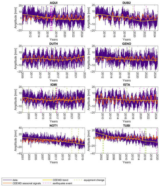
Figure 2.
CEEMD decomposition of the U component time series of AQUI, DUB2, DUTH, GENO, IGMI, ISTA, NOT1, and TUBI stations into seasonal signals and trend.
Similar results were also obtained for the remaining stations analyzed, where no significant discontinuities resulting from events were noted. However, special cases will be the stations where significant discontinuities were noted (Figure 3).
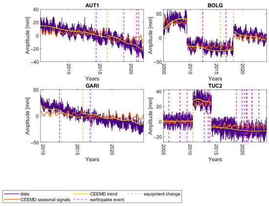
Figure 3.
CEEMD decomposition of the U component time series of AUT1, BLOG, GARI, and TUC2 stations into seasonal signals and trend.
In the case of stations for which significant discontinuities and earthquakes were noted and thus trends were modeled for individual time intervals, the trends have a more pronounced nonlinear character (Figure 3). Moreover, the trends modeled using the CEEMD method can be noticeably described by exponential and logarithmic functions, e.g., station BOLG. It should also be noted that the trends modeled using the CEEMD method for short time intervals, such as in the case of TUC2 and the period of 3 years, may be insignificant.
To assess the suitability of the CEEMD method for modeling nonlinear trends, a comparative analysis was performed with nonlinear trends estimated using the SSA method. Figure 4 presents an example comparison of the obtained trends for the AQUI, GENO, IZMI, and ZADA stations. This shows that the trends determined by the SSA method are more nonlinear than the trends estimated by the CEEMD method. However, these nonlinearities are not associated with earthquake occurrence. This is particularly evident in the case of the GENO station, for which no earthquakes were recorded during the period under consideration, and the trend determined by the SSA method is clearly nonlinear. In the case of the AQUI and IZMI stations, the trends modeled by the SSA method are also more pronounced as nonlinear than those modeled by the CEEMD method. However, this nonlinearity occurs not only in the vicinity of earthquakes but also during periods without seismic activity.
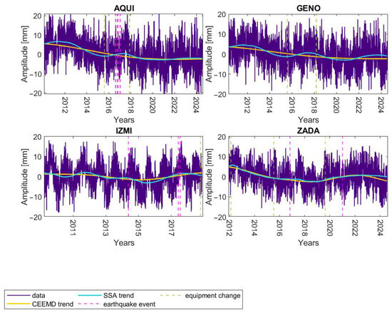
Figure 4.
Nonlinear trends modeled using the CEEMD and SSA methods for AQUI, GENO, IZMI, and ZADA stations.
In a comparative analysis of trends estimated by the CEEMD method with those determined by the SSA method, correlation coefficients and RMSE were also determined (Figure 5). In 68% of cases, the correlation coefficients are above 0.90, while in 16% of cases, they are in the range of 0.80 to 0.90. The lowest correlation coefficient values are noted for stations DUTH, ISTA, ORID, and PADO, amounting to 0.61, 0.49, 0.60, and 0.15, respectively. In the case of PADO, the low correlation coefficient value is a consequence of the negative correlation between trends in the period before the discontinuity caused by equipment change. In turn, considering the obtained RMSE values, in 56% of cases, they reach values below 1 mm. The highest RMSE values are noted for the BOLG, GARI, and ORID stations, at 4.11, 5.47, and 3.27, respectively. Only the ORID station has also one of the lowest correlation coefficients. However, for the BOLG and GARI stations, the relatively high RMSE values may be due to the periods for which the trends were estimated. For the BOLG station, trends were estimated for three-time intervals of approximately 4.5, 8, and 6.5 years, and for the GARI station, for two-time intervals of approximately 5.5 and 9.5 years.
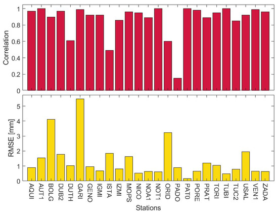
Figure 5.
Values of correlation coefficients and RMSE between trends estimated using the CEEMD as well as SSA method.
The values of the mean standard deviation determined by the bootstrap method for the trend estimated by the CEEMD and SSA methods (Figure 6) are, in both cases, at the level of approximately 1–3 mm. At the same time, the highest values of the mean standard deviation were noted for the AUT1, GARI, NOT1, and TUBI stations, and they were 5.81, 6.64, 6.28, and 6.81 mm, respectively, for the CEEMD method, and 5.76, 6.32, 6.26, and 6.81 mm, respectively, for the SSA method. In the case of the GARI and TUBI stations, the estimated trends are clearly nonlinear. In the case of the TUBI station, only two earthquake events were noted, but they occurred at the end of the analyzed periods, i.e., in 2014 and 2019. In the case of the GARI station, in the considered period, only one earthquake occurred in 2016, after which a change in the trend is noticeable. Moreover, in the period without events, lasting over 10 years, the determined trend is also nonlinear. In the case of the NOT1 station, there were no events related to earthquakes in a period of almost 15 years, and the determined trend is close to linear but with small local changes. The lowest mean standard deviation values were noted for stations NOA1, PADO, and DUTH, amounting to 0.75, 1.08, and 0.62 mm for the CEEMD method, and 0.43, 0.66, and 1.25 mm for the SSA method, respectively. In these cases, the determined trends are closest to linear, with slopes below 1 mm. The DUTH and PADO stations also had the lowest correlation coefficients between the trend estimated using the CEEMD and SSA methods.
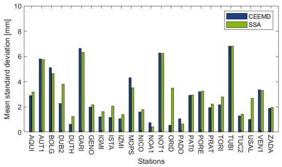
Figure 6.
Mean bootstrap standard deviation values for the trend determined by the CEEMD and SSA method.
Therefore, the bootstrap estimated mean standard deviation values are unlikely to show any relationship with the estimated trend. However, it can be noticed that higher values of the mean standard deviation were obtained mainly for stations where significant discontinuities occurred, and therefore trends were estimated for shorter time intervals, e.g., stations AUT1, BOLG, GARI, MOPS, and VEN1, but there are also exceptions to this, such as stations PADO, PRAT, TORI, or TUC2. Moreover, the mean standard deviation values, interpreted as the uncertainty of the estimated trends using the CEEMD method, are slightly lower than the uncertainties estimated in the same way but for trends determined by the SSA method. The mean value of the mean standard deviation is 2.72 mm for the CEEMD method and 3.03 mm for the SSA method, while the medians are 2.00 mm and 2.79 mm, respectively. The obtained mean standard deviation values for the estimated trends do not differ significantly from the annual uncertainties estimated using other methods [e.g., 11, 19]. Relatively high standard deviation values, as in the case of stations AUT1, GARI, NOT1, or TUBI, may be a consequence of estimating a time-varying trend and using the time-frequency method. However, in these cases, high mean standard deviation values were obtained for both the CEEMD and SSA methods. It should also be noted that failure to take into account discontinuities in the time series related to equipment changes would have a significant impact on the increase in the mean standard deviation. Therefore, trend analysis should pay particular attention to emerging discontinuities, regardless of their source, which was also confirmed in previous studies [50].
To compare the estimated time-varying trend with the linear one, a least squares (LS) linear trend was also fitted to the trend obtained by CEEMD. Due to the fact that the trends estimated by the CEEMD method do not differ significantly from those estimated by the SSA method, linear fitting was performed only in the case of the CEEMD method. Figure 7 shows the CEEMD trends together with the LS estimated trend. Figure 8 also shows the trends estimated by the LS and CEEMD methods along with fitting the linear trend to the nonlinear CEEMD trend, but for stations where significant discontinuities were noted and the trends were estimated for individual time intervals. Figure 7 and Figure 8 also show the changes in equipment and earthquakes noted near the station, according to the information provided in the NGL service [39].
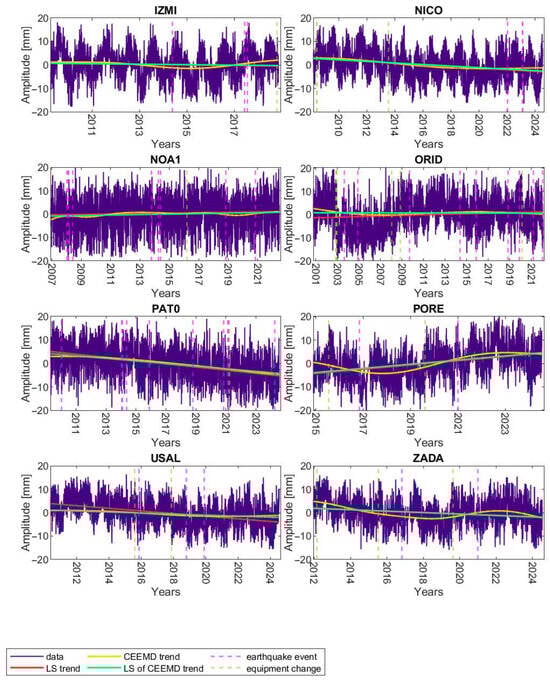
Figure 7.
LS trends, CEEMD trends, and LS of CEEMD trends determined for IZMI, NICO, NOA1, ORID, PAT0, PORE, USAL, and ZADA stations and the U component.
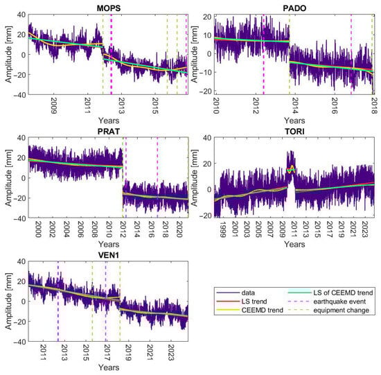
Figure 8.
LS trends, CEEMD trends and LS of CEEMD trends determined for MOPS, PADO, PRAT, TORI and VEN1 stations and the U component.
In all the cases, the discrepancies between the nonlinear and linear trend are at the level of several millimeters, and the nonlinearity is usually visible in the vicinity of the occurrence of earthquakes noticed near the station. Most often, the occurrence of an earthquake causes changes in both the value and the sign of the direction of the nonlinear trend (Figure 7, e.g., stations IZMI, PORE, VEN1, ZADA). On the other hand, if in the considered period there are no earthquake events near the station (e.g., station IZMI, NICO, PRAT), then there is practically no discrepancy between the linear and nonlinear trends. Nevertheless, in some cases, there are nonlinear changes in the trend, which are not accompanied by events related to the earthquakes (e.g., station VEN1, TORI). However, it should be taken into account that there may have been changes because of an earthquake or other phenomena which took place at a further distance from the station and were not noticed. Additionally, sometimes nonlinearity becomes visible at the beginning of the time series, e.g., MOPS station, where data from the station have been available since April 2007, or BOLG and GARI (Figure 3), where data are available from September 2004 and May 2009, respectively. Therefore, the initial nonlinearity of the time series may be the effect of the station foundation and stabilization and may not be related to geophysical factors. The influence of correlated noise in GPS time series also cannot be excluded, which may affect the determination of the trend in the CEEMD decomposition as well as in the modeling of the linear trend. Also, as is well known, estimating the vertical component is more problematic than estimating the horizontal components.
Moreover, in the case of the trend fitted to the original data using the LS method, the standard error of the trend fit in most cases reaches values of 5–6 mm (Table 2). The mean value of the standard error in the analyzed set of stations reaches 5.89 mm, while the median is 5.85 mm. Thus, the standard error of the trend fit using the LS method was approximately twice as high as the standard deviation for nonlinear trends estimated using the bootstrap method.
Table 2.
The slope values provided by the NGL service for each station and estimated using the MIDAS method [11] as well as for the linear trend fitted with the LS method to the original time series, together with standard error of LS trend fit, and for the trend fitted with the LS method to the nonlinear trend obtained with the CEEMD method and the RMSE values between the CEEMD trend and the linear trend fitted to it.
In turn, the linear trend fitted using the LS method to the original time series does not differ significantly in terms of the slope coefficient of the curve from the linear trend fitted also using the LS method to the CEEMD trend. Thanks to the determination of trends using CEEMD, it is possible to notice the occurrence of co-seismic displacement or breaks associated with earthquakes at the station position. Similar results were also obtained by Heflin et al. [14], stating that in general, after earthquakes, stations return to their long-term movements after 2–3 years, although there are some exceptions. Table 2 summarizes the values of the slope of the curve provided by the NGL service for each station and estimated using the MIDAS method [11], as well as for the linear trend fitted to the original time series using the LS method and for the trend fitted to the nonlinear trend obtained using the CEEMD method. The root mean square error (RMSE) values between the CEEMD trend and the linear trend fitted to it using the LS method were also compared.
For most stations, the slope value of the curve expressed per year and estimated using the MIDAS and LS methods assumes values in a comparable range. The discrepancies resulted mainly from different time intervals for which the trends were estimated and the estimation methods used. In turn, when considering the slope values of the curve from the LS method and LS fitted into the CEEMD trend, no significant discrepancies are noticeable, with the largest occurring for the BOLG and TORI stations. In the case of the TORI station, the discrepancy is also in the sign of the slope; however, the estimated trend should be considered insignificant due to the time interval for which it was estimated, which was less than 1.5 years. The RMSE assumes values from 0.10 to 2.96 mm, depending on the station. At the same time, the highest RMSE values were observed for the BOLG, MOPS, and TORI stations, which allows us to conclude that in these cases, the determined trend may have the most noticeable nonlinear character. In turn, the lowest RMSE values were noted for the TUC2 and USAL stations. In these cases, the trend estimated by the CEEMD method is linear and the slope of the trend line is small.
4. Discussion
The commonly used methods for determining linear trends in GPS time series are methods based on the least squares [11,12,13]. However, estimating linear velocities from time series of GPS station positions, which contain discontinuities, is biased [37,55]. Thus, modeling trends in GPS time series using the CEEMD method is a new possibility in the analysis of time-varying characteristics of GPS time series trends, in particular for their geophysical interpretation. This is also actually one of the most important topics in modern geodesy, as the current implementation of the International Terrestrial Reference System (ITRS) in the form of ITRF2020 already includes improved modeling of nonlinear station motions to better characterize the shape of the Earth’s deforming surface [47]. In ITRF2020, the nonlinearity of station velocity is implemented by a model composed of a linear function, annual and semi-annual signals, and a function describing post-seismic deformation (PSD).
Geophysical events such as earthquakes can therefore cause crustal deformations on local and regional scales, which in turn will manifest themselves as local nonlinearities in GPS time series. Moreover, discontinuities due to equipment changes or earthquake events have been observed to make it difficult to estimate geophysical signals such as uplift rates and seasonal loading signals [54]. Our results confirm the observations of Bogusz [9] that the nonlinearity of GPS station velocities is not obvious, but cannot be excluded, especially in regions of tectonic activity. Moreover, GPS time series may contain variable velocities on shorter time scales, caused by earthquakes and the accompanying post-seismic deformation of the Earth’s crust, which in turn is consistent with the results of Klos et al. [8]. Also, Heflin et al. [14] noted that the occurrence of an earthquake causing a break or co-seismic displacement causes changes in the velocity of the stations, which return to their long-term movements after 2–3 years, although there are some exceptions. Thus, post-seismic relaxations are usually modeled in GPS time series as logarithmic and exponential functions [52,53]. The occurrence of nonlinearities in GPS time series can also be related to volcanic activity [56], however, in the cases considered in this study, none of the stations are located in close proximity to an active volcano. Moreover, in the case of stations such as DUTH, ISTA, NICO, NOA1, NOT1, PAT0, TUBI, and USAL, which are located at the tectonic plate boundary as well as subduction area (Figure 1), the time series may contain signals resulting from the nonlinear dynamics of microplates [10]. In this case, it is also necessary to take into account the study by Banerejee [2], which showed that GPS stations located near a subduction zone that has ruptured may undergo rapid post-seismic relaxation in the years following the event.
Taking these aspects into account, in the case of stations located in areas of seismic activity as well as in the boundary areas of tectonic plates, it becomes important to use nonlinear trend estimation methods. Thus, using the CEEMD method to model nonlinear trends will not only enable the analysis of the impact of listed seismic activities on changes in the position of GPS stations but may also allow the detection of phenomena influencing these changes. At the same time, further research should focus on the use of modeled time-varying signals in correlation analyses with geophysical signals, because the CEEMD method itself can be applied not only to GPS time series but also in the analysis of seismic signals [57] or sea level studies [58].
An undoubted disadvantage of the CEEMD method, and thus its limitation, is the lack of uncertainty estimation of individual IMFs. In this case, it is necessary to estimate the uncertainty using other statistical methods, which, as shown in this study, can be achieved using, e.g., the bootstrap method. However, it should be noted that the use of bootstrap simulation is time consuming, especially when combined with the CEEMD method, as in this study. For example, estimating the mean standard deviation for the trend determined by the CEEMD method and a GPS time series of 5273 days (14.4 years) and 200 times of sampling with replacement, the computation time was 453 s.
Nevertheless, the iterative nature of CEEMD leading to the lack of strict mathematical relationships may be a limitation of this method, especially in accurate analyses of GPS time series, while at the same time providing opportunities for the proper interpretation of the non-stationary characteristics of these series. It should also be noted that the CEEMD method allows for simultaneous denoising, modeling of time-varying periodic oscillations, and a nonlinear trend, which is an undoubted advantage in analyses of time series of GPS station positions. The quality of the data used and its impact on the values of estimated time-varying trends will also be important. Moreover, the CEEMD method, like most time-frequency methods, has its limitations, especially in terms of the accuracy of the obtained models due to the common dependence that a good solution in the time domain will result in a worse one in the frequency domain and vice versa.
In further analyses, in order to enhance the effectiveness of the CEEMD method in estimating the trend, one can additionally apply wavelet denoising and then perform the CEEMD decomposition. The usefulness of this type of procedure in the analysis of seasonal signals in GNSS time series was demonstrated in the work of Wnęk and Kudas [32].
5. Conclusions
The conducted studies have shown the usefulness of the CEEMD method to model nonlinear trends in GPS time series, which may be the result of seismic activity and accompanying post-seismic deformations of the Earth’s crust. A comparative analysis of the nonlinear trends estimated using the CEEMD method with the trends determined using the SSA method showed that both methods were compatible, with an average correlation coefficient for the analyzed set of stations of 0.87. In turn, comparison of the determined nonlinear trends with their linear counterparts allows us to state that the nonlinearities of the trends are at a level of 0.1 to 3.0 mm, depending on the station, its location, as well as the occurrence of earthquake events. Moreover, in the absence of earthquakes or their negligible impact, the estimated trends are close to linear.
An undeniable disadvantage of the CEEMD method is the lack of an estimate of the uncertainty of the modeled trends. Therefore, in this study, the bootstrap statistical method was successfully proposed to estimate the mean standard deviation of the determined trends. In the case of the considered time series of station positions, the average value of the standard deviation estimated by the bootstrap method is, on average, at the level of 1–3 mm, which should be considered a low value in this type of estimation. Moreover, in the future, in the analyses of GPS time series, statistical methods such as bootstrap can also be used to estimate the uncertainty not only of the trend but also of the individual IMFs obtained in the CEEMD decomposition process.
Author Contributions
Conceptualization, A.W.; methodology, A.W.; validation, A.W. and D.K.; formal analysis, A.W.; data curation, A.W.; writing—original draft preparation, A.W.; writing—review and editing, D.K.; visualization, A.W. and D.K. All authors have read and agreed to the published version of the manuscript.
Funding
The APC was funded by the Ministry of Science and Higher Education from a subsidy for the University of Agriculture in Krakow (Department of Geodesy).
Data Availability Statement
GPS station position time series developed by NGL are openly available at: https://geodesy.unr.edu/NGLStationPages/GlobalStationList (accessed on 20 April 2025). Steps for all stations are available at: https://geodesy.unr.edu/NGLStationPages/steps.txt (accessed on 20 April 2025).
Acknowledgments
We thank the Nevada Geodetic Laboratory (NGL) for providing the daily GPS station position time series.
Conflicts of Interest
The authors declare no conflicts of interest.
Abbreviations
The following abbreviations are used in this manuscript:
| GPS | Global Positioning System |
| CEEMD | Complementary Ensemble Empirical Mode Decomposition |
| NGL | Nevada Geodetic Laboratory |
| GNSSs | Global Navigation Satellite Systems |
| RMSE | Root Mean Square Error |
| MIDAS | Median Interannual Difference Adjusted for Skewness |
| MLE | Maximum Likelihood Estimation |
| SSA | Singular Spectrum Analysis |
| PPP | Precise Point Positioning |
| EPN | EUREF Permanent Network |
| MAD | Median Absolute Deviation |
| EMD | Empirical Mode Decomposition |
| IMFs | Intrinsic Mode Functions |
| ITRF | International Terrestrial Reference Frame |
| LSs | Last Squares |
| ITRS | International Terrestrial Reference System |
| PSD | Post-Seismic Deformation |
| USGS | U. S. Geological Survey |
References
- Blewitt, G.; Lavallée, D.; Clarke, P.; Nurutdinov, K. A new global mode of Earth deformation: Seasonal cycle detected. Science 2001, 294, 2342–2345. [Google Scholar] [CrossRef]
- Banerjee, P.; Pollitz, F.F.; Nagarajan, B.; Burgmann, R. Coseismic slip distributions of the 26 December 2004 Sumatra-Andaman and 28 March 2005 Nias earthquakes from GPS static offsets. Bull. Seismol. Soc. Am. 2007, 97, S86–S102. [Google Scholar] [CrossRef]
- Tregoning, P.; Burgette, R.; McClusky, S.C.; Lejeune, S.; Watson, C.S.; McQueen, H. A decade of horizontal deformation from great earthquakes. J. Geophys. Res. 2013, 118, 2371–2381. [Google Scholar] [CrossRef]
- Nistor, S.; Suba, N.S.; El-Mowafy, A.; Apollo, M.; Malkin, Z.; Nastase, E.I.; Kudrys, J.; Maciuk, K. Implication between Geophysical Events and the Variation of Seasonal Signal Determined in GNSS Position Time Series. Remote Sens. 2021, 13, 3478. [Google Scholar] [CrossRef]
- Dong, D.; Fang, P.; Bock, Y.; Cheng, M.K.; Miyazaki, S.I. Anatomy of apparent seasonal variations from GPS-derived site position time series. J. Geophys. Res. Solid Earth 2002, 107, ETG-9. [Google Scholar] [CrossRef]
- Kermarrec, G.; Maddanu, F.; Klos, A.; Proietti, T.; Bogusz, J. Modeling trends and periodic components in geodetic time series: A unified approach. J. Geod. 2024, 98, 17. [Google Scholar] [CrossRef]
- Oelsmann, J.; Passaro, M.; Sánchez, L.; Dettmering, D.; Schwatke, C.; Seitz, F. Bayesian modelling of piecewise trends and discontinuities to improve the estimation of coastal vertical land motion: DiscoTimeS: A method to detect change points in GNSS, satellite altimetry, tide gauge and other geophysical time series. J. Geod. 2022, 96, 62. [Google Scholar] [CrossRef]
- Klos, A.; Kusche, J.; Fenoglio-Marc, L.; Bos, M.S.; Bogusz, J. Introducing a vertical land motion model for improving estimates of sea level rates derived from tide gauge records affected by earthquakes. GPS Solut. 2019, 23, 102. [Google Scholar] [CrossRef]
- Bogusz, J. Geodetic aspects of GPS permanent station nonlinearity studies. Acta Geodyn. Geomater. 2015, 12, 180. [Google Scholar] [CrossRef]
- Hobbs, B.; Ord, A. Nonlinear dynamical analysis of GNSS data: Quantification, precursors and synchronisation. Prog. Earth Planet. Sci. 2018, 5, 36. [Google Scholar] [CrossRef]
- Blewitt, G.; Kreemer, C.; Hammond, W.C.; Gazeaux, J. MIDAS robust trend estimator for accurate GPS station velocities without step detection. J. Geophys. Res. Solid Earth 2016, 121, 2054–2068.b. [Google Scholar] [CrossRef]
- Williams, S.D.P. CATS: GPS coordinate time series analysis software. GPS Solut. 2008, 12, 147–153. [Google Scholar] [CrossRef]
- Bos, M.S.; Fernandes, R.M.S.; Williams, S.D.P.; Bastos, L. Fast error analysis of continuous GNSS observations with missingdata. J. Geod. 2013, 87, 351–360. [Google Scholar] [CrossRef]
- Heflin, M.; Donnellan, A.; Parker, J.; Lyzenga, G.; Moore, A.; Ludwig, L.G.; Rundle, J.; Wang, J.; Pierce, M. Automated estimation and tools to extract positions, velocities, breaks, and seasonal terms from daily GNSS measurements: Illuminating nonlinear Salton Trough deformation. Earth Space Sci. 2020, 7, e2019EA000644. [Google Scholar] [CrossRef]
- Bos, M.S.; Bastos, L.; Fernandes, R.M.S. The influence of seasonal signals on the estimation of the tectonic motion in short continuous GPS time-series. J. Geodyn. 2010, 49, 205–209. [Google Scholar] [CrossRef]
- Klos, A.; Bos, M.S.; Bogusz, J. Detecting time-varying seasonal signal in GPS position time series with different noise levels. GPS Solut. 2018, 22, 21. [Google Scholar] [CrossRef]
- Chen, Q.; van Dam, T.; Sneeuw, N.; Collilieux, X.; Weigelt, M.; Rebischung, P. Singular spectrum analysis for modeling seasonal signals from GPS time series. J. Geodyn. 2013, 72, 25–35. [Google Scholar] [CrossRef]
- Yeh, J.R.; Shieh, J.S.; Huang, N.E. Complementary ensemble empirical mode decomposition: A novel noise enhanced data analysis method. Adv. Adapt. Data Anal. 2010, 2, 135–156. [Google Scholar] [CrossRef]
- Ji, K.; Shen, Y.; Wang, F. Signal Extraction from GNSS Position Time Series Using Weighted Wavelet Analysis. Remote Sens. 2020, 12, 992. [Google Scholar] [CrossRef]
- Kaczmarek, A.; Kontny, B. Identification of the Noise Model in the Time Series of GNSS Stations Coordinates Using Wavelet Analysis. Remote Sens. 2018, 10, 1611. [Google Scholar] [CrossRef]
- Gruszczynska, M.; Klos, A.; Gruszczynski, M.; Bogusz, J. Investigation of time-changeable seasonal components in the GPS height time series: A case study for Central Europe. Acta. Geodyn. Geomater. 2016, 13, 281–289. [Google Scholar] [CrossRef]
- Khazraei, S.M.; Amiri-Simkooei, A.R. On the application of Monte Carlo singular spectrum analysis to GPS position time series. J. Geod. 2019, 93, 1401–1418. [Google Scholar] [CrossRef]
- Ji, K.; Shen, Y.; Chen, Q.; Wang, F. Extended singular spectrum analysis for processing incomplete heterogeneous geodetic time series. J. Geod. 2023, 97, 74. [Google Scholar] [CrossRef]
- Ji, K.; Shen, Y.; Wang, F.; Chen, Q. An efficient improved singular spectrum analysis for processing GNSS position time series with missing data. Geophys. J. Int. 2025, 240, 189–200. [Google Scholar] [CrossRef]
- Wnęk, A.; Kudas, D. Modeling seasonal oscillations in GNSS time series with Complementary Ensemble Empirical Mode Decomposition. GPS Solut. 2022, 26, 101. [Google Scholar] [CrossRef]
- Li, Y.; Xu, C.; Yi, L.; Fang, R. A data-driven approach for denoising GNSS position time series. J. Geod. 2018, 92, 905–922. [Google Scholar] [CrossRef]
- Li, Y.; Han, L.; Yi, L.; Zhong, S.; Chen, C. Feature extraction and improved denoising method for nonlinear and nonstationary high-rate GNSS coseismic displacements applied to earthquake focal mechanism inversion of the El Mayor-Cucapah earthquake. Adv. Space Res. 2021, 68, 3971–3991. [Google Scholar] [CrossRef]
- Montillet, J.P.; Tregoning, P.; McClusky, S.; Yu, K. Extracting white noise statistics in GPS coordinate time series. IEEE Geosci. Remote Sens. Lett. 2012, 10, 563–567. [Google Scholar] [CrossRef]
- Niu, Y.; Ye, Y.; Zhao, W.; Shu, J. Dynamic monitoring and data analysis of a long-span arch bridge based on high-rate GNSS-RTK measurement combining CF-CEEMD method. J. Civ. Struct. Health Monit. 2021, 11, 35–48. [Google Scholar] [CrossRef]
- Yang, B.; Yang, Z.; Tian, Z.; Liang, P. Weakening the Flicker Noise in GPS Vertical Coordinate Time Series Using Hybrid Approaches. Remote Sens. 2023, 15, 1716. [Google Scholar] [CrossRef]
- Li, Y.; Han, L.; Liu, X. Accuracy Enhancement and Feature Extraction for GNSS Daily Time Series Using Adaptive CEEMD-Multi-PCA-Based Filter. Remote Sens. 2023, 15, 1902. [Google Scholar] [CrossRef]
- Wnęk, A.; Kudas, D. Application of combination of denoising methods and Complementary Ensemble Empirical Mode Decomposition in GNSS time series analysis. GPS Solut. 2025, 29, 141. [Google Scholar] [CrossRef]
- Blewitt, G.; Hammond, W.C.; Kreemer, C. Harnessing the GPS data explosion for interdisciplinary science. Eos 2018, 99, e2020943118. [Google Scholar] [CrossRef]
- Klein, J.; Valkama, M.; Staudt, M.; Schmidt-Thomé, P.; Kallio, H. ESPON-TITAN: Territorial patterns of natural hazards in Europe. Nat. Hazards 2024, 1–23. [Google Scholar] [CrossRef]
- U. S. Geological Survey. Search Earthquake Catalog. Available online: https://earthquake.usgs.gov/earthquakes/search (accessed on 14 July 2025).
- Bird, P. An updated digital model of plate boundaries. Geochem. Geophys. Geosyst. 2003, 4, 1027. [Google Scholar] [CrossRef]
- Gazeaux, J.; Williams, S.; King, M.; Bos, M.; Dach, R.; Deo, M.; Moore, A.W.; Ostini, L.; Petrie, E.; Roggero, M.; et al. Detecting offsets in GPS time series: First results from the detection of offsets in GPS experiment. J. Geophys. Res. Solid Earth 2013, 118, 2397–2407. [Google Scholar] [CrossRef]
- Tretyak, K.; Dosyn, S. Study of vertical movements of the European crust using tide gauge and GNSS observations. Rep. Geod. Geoinform. 2014, 97, 112–131. [Google Scholar] [CrossRef]
- NGL Steps 2024. Available online: http://geodesy.unr.edu/NGLStationPages/steps.txt (accessed on 20 April 2025).
- Huang, N.E.; Shen, Z.; Long, S.R.; Wu, M.C.; Shih, H.H.; Zheng, Q.; Yen, N.C.; Tung, C.C.; Liu, H.H. The empirical mode decomposition and the Hilbert spectrum for nonlinear and nonstationary time series analysis. Proc. R. Soc. Lond. Ser. A Math. Phys. Eng. Sci. 1998, 454, 903–995. [Google Scholar] [CrossRef]
- Huang, Y.; Schmitt, F.G.; Lu, Z.; Liu, Y. Analysis of daily river flow fluctuations using empirical mode decomposition and arbitrary order Hilbert spectral analysis. J. Hydrol. 2009, 373, 103–111. [Google Scholar] [CrossRef]
- Huang, N.E.; Wu, Z. A review on Hilbert–Huang transform: Method and its applications to geophysical studies. Rev. Geophys. 2008, 46, RG2006. [Google Scholar] [CrossRef]
- Wu, Z.; Huang, N.E. Ensemble empirical mode decomposition: A noise-assisted data analysis method. Adv. Adapt. Data Anal. 2009, 1, 1–41. [Google Scholar] [CrossRef]
- Efron, B.; Tibshirani, R. Bootstrap methods for standard errors, confidence intervals, and other measures of statistical accuracy. Stat. Sci. 1986, 1, 54–75. [Google Scholar] [CrossRef]
- Efron, B.; Tibshirani, R.J. An Introduction to the Bootstrap; Chapman and Hall/CRC: Boca Raton, FL, USA, 1994. [Google Scholar]
- Altamimi, Z.; Rebischung, P.; Métivier, L.; Collilieux, X. ITRF2014: A new release of the International Terrestrial Reference Frame modeling nonlinear station motions. J. Geophys. Res. Solid Earth 2016, 121, 6109–6131. [Google Scholar] [CrossRef]
- Altamimi, Z.; Rebischung, P.; Collilieux, X.; Métivier, L.; Chanard, K. ITRF2020: An augmented reference frame refining the modeling of nonlinear station motions. J. Geod. 2023, 97, 47. [Google Scholar] [CrossRef]
- The MathWorks Inc. MATLAB, Version: 23.2.0.2485118 (R2023b) Update 6; The MathWorks Inc.: Natick, MA, USA, 2023; Available online: https://www.mathworks.com (accessed on 20 April 2025).
- Herring, T.A.; Melbourne, T.I.; Murray, M.H.; Floyd, M.A.; Szeliga, W.M.; King, R.W.; Phillips, D.A.; Puskas, C.M.; Santillan, M.; Wang, L. Plate Boundary Observatory and related networks: GPS data analysis methods and geodetic products. Rev. Geophys. 2016, 54, 759–808. [Google Scholar] [CrossRef]
- He, X.; Bos, M.S.; Montillet, J.-P.; Fernandes, R.; Melbourne, T.; Jiang, W.; Li, W. Spatial Variations of Stochastic Noise Properties in GPS Time Series. Remote Sens. 2021, 13, 4534. [Google Scholar] [CrossRef]
- Kowalczyk, K.; Rapinski, J. Verification of a GNSS time series discontinuity detection approach in support of the estimation of vertical crustal movements. ISPRS Int. J. Geo-Inf. 2018, 7, 149. [Google Scholar] [CrossRef]
- Kreemer, C.; Blewitt, G.; Maerten, F. Co- and postseismic deformation of the 28 March 2005 Nias Mw 8.7 earthquake from continuous GPS data. Geophys. Res. Lett. 2006, 33, L07307. [Google Scholar] [CrossRef]
- Tobita, M. Combined logarithmic and exponential function model for fitting postseismic GNSS time series after 2011 Tohoku-Oki earthquake. Earth Planets Space 2016, 68, 41. [Google Scholar] [CrossRef]
- Williams, S.D.P.; Bock, Y.; Fang, P.; Jamason, P.; Nikolaidis, R.M.; Prawirodirdjo, L.; Miller, M.; Johnson, D.J. Error analysis of continuous GPS position time series. J. Geophys. Res. 2004, 109, B03412. [Google Scholar] [CrossRef]
- Montillet, J.P.; Williams, S.D.P.; Koulali, A.; McClusky, S.C. Estimation of offsets in GPS time-series and application to the detection of earthquake deformation in the far-field. Geophys. J. Int. 2015, 200, 1207–1221. [Google Scholar] [CrossRef]
- Clarke, D.; Brenguier, F.; Froger, J.-L.; Shapiro, N.M.; Peltier, A.; Staudacher, T. Timing of a large volcanic flank movement at Piton de la Fournaise Volcano using noise-based seismic monitoring and ground deformation measurements. Geophys. J. Int. 2013, 195, 1132–1140. [Google Scholar] [CrossRef]
- Zhang, P.; Dai, Y.; Zhang, H.; Wang, C.; Zhang, Y. Combining CEEMD and recursive least square for the extraction of time-varying seismic wavelets. J. Appl. Geophys. 2019, 170, 103854. [Google Scholar] [CrossRef]
- Shao, Q.; Li, W.; Hou, G.; Han, G.; Wu, X. Mid-term simultaneous spatiotemporal prediction of sea surface height anomaly and sea surface temperature using satellite data in the South China Sea. IEEE Geosci. Remote Sens. Lett. 2020, 19, 1501705. [Google Scholar] [CrossRef]
Disclaimer/Publisher’s Note: The statements, opinions and data contained in all publications are solely those of the individual author(s) and contributor(s) and not of MDPI and/or the editor(s). MDPI and/or the editor(s) disclaim responsibility for any injury to people or property resulting from any ideas, methods, instructions or products referred to in the content. |
© 2025 by the authors. Licensee MDPI, Basel, Switzerland. This article is an open access article distributed under the terms and conditions of the Creative Commons Attribution (CC BY) license (https://creativecommons.org/licenses/by/4.0/).