Article

A Deep Transfer Contrastive Learning Network for Few-Shot Hyperspectral Image Classification

Faculty of Computer Science and Technology, Hainan University, Haikou 570228, China
*
Author to whom correspondence should be addressed.
Remote Sens. 2025, 17(16), 2800; https://doi.org/10.3390/rs17162800
Submission received: 11 June 2025 / Revised: 7 August 2025 / Accepted: 7 August 2025 / Published: 13 August 2025

Abstract

Over recent decades, the hyperspectral image (HSI) classification landscape has undergone significant transformations driven by advances in deep learning (DL). Despite substantial progress, few-shot scenarios remain a significant challenge, primarily due to the high cost of manual annotation and the unreliability of visual interpretation. Traditional DL models require massive datasets to learn sophisticated feature representations, hindering their full potential in data-scarce contexts. To tackle this issue, a deep transfer contrastive learning network is proposed. A spectral data augmentation module is incorporated to expand limited sample pairs. Subsequently, a spatial–spectral feature extraction module is designed to fuse the learned feature information. The weights of the spatial feature extraction network are initialized with knowledge transferred from source-domain pretraining, while the spectral residual network acquires rich spectral information. Furthermore, contrastive learning is integrated to enhance discriminative representation learning from scarce samples, effectively mitigating obstacles arising from the high inter-class similarity and large intra-class variance inherent in HSIs. Experiments on four public HSI datasets demonstrate that our method achieves competitive performance against state-of-the-art approaches.

1. Introduction

Hyperspectral images (HSIs) captured by airborne or spaceborne sensors comprise plenty of narrow and continuous spectral channels, which can provide rich spectral and spatial information [1,2]. In the past few years, the HSI classification task has received widespread attention [3,4], and it has found extensive applications in fields such as smart agriculture [5], environmental monitoring [6], mineral surveys [7], etc. Despite this progress, accurate classification remains a formidable challenge, especially with limited training samples [8]. Consequently, few-shot HSI classification has emerged as an active area of research.
HSI data collection and labeling present persistent bottlenecks in hyperspectral remote sensing applications [9]. Initially, hyperspectral sensors produce an immense volume of data, with each pixel exhibiting responses across a spectrum ranging from dozens to hundreds of bands. This necessitates a substantial number of labeled samples to adequately represent the data. The labor cost of HSI labeling a single scene is high, and the interpretation of HSIs is also a specialized task demanding profound expertise; only professionals with extensive field knowledge have the capability to precisely identify and classify the specific materials and objects in the imagery. Additionally, the collection of some HSI data involves inaccessible areas, which poses significant challenges for ground-truth surveys and sample collection. Thus, the availability of labeled HSI samples is currently quite constrained.
In previous research, scholars dedicated their efforts to the meticulous design of feature extraction and selection processes, aiming to address the difficulties arising from data scarcity. A set of techniques was adopted to effectively harness the discriminative power of features, e.g., a histogram of oriented gradients [10], principal component analysis [11], and local binary patterns [12]. As research has progressed, some classification algorithms have been exploited to improve the accuracy, such as random forest [13], support vector machine (SVM) [14], k-nearest neighbors [15], multinomial logistic regression [16], and so on. However, these algorithms can only extract shallow spectral and spatial features from HSIs and lack sufficient generalization and representation capabilities when dealing with limited HSI samples.
Deep learning (DL) techniques, particularly convolutional neural networks [17], stacked autoencoders [18], and deep belief networks [19], have demonstrated remarkable capabilities and achieved breakthroughs in the challenging task of few-shot hyperspectral image (HSI) classification over recent years [20]. These DL classification models can automatically learn high-level feature representations of the hierarchical features of known samples and effectively handle the large spatial variability and high dimensionality of HSIs. For instance, Li et al. [21] introduced a lightweight 3D-CNN framework that directly processes raw HSI cubes, eliminating preprocessing needs while efficiently extracting joint spectral–spatial features with minimal parameters. Zhong et al. [22] introduced an end-to-end spectral–spatial residual network (SSRN) with dedicated residual blocks, which processes raw HSI cubes through identity mapping and batch normalization to mitigate gradient vanishing in deep 3D-CNNs. However, model performance is empirically observed to correlate with training sample abundance. Consequently, the application of traditional DL models in scenarios where training samples are limited is prone to result in overfitting and suboptimal classification performance.
Given the pressing need for solutions to few-shot HSI classification tasks, researchers have studied them for more than a decade [23,24,25,26,27,28,29]. Among these studies, some have focused on the perspective of extending limited sample sets. Haut et al. [24] adopted random occlusion of pixels in different rectangular spatial regions to generate training samples. Zhu et al. [25] leveraged GAN-generated adversarial samples with real data to fine-tune discriminative CNNs. However, these methods may introduce noise during data enhancement and have difficulty in fully considering spatial–spectral information. On the other hand, some scholars consider deep learning to provide better representations from insufficient data. In [27], an adaptive graph convolution extracts multi-scale patch features, while a BiLSTM captures cross-scale spectral–spatial dependencies. Jiang and Jia [30] applied the Siamese Network with depth separable convolution to capture relationships between data. These deep models contain numerous trainable parameters (e.g., network weights), often causing training difficulties that present significant practical challenges.
To resolve this matter, some frameworks have been shown to have more potential, such as meta-learning [21,22,23,24,25,26,27,28,29,30,31,32,33], self-supervised learning [34], transfer learning [35,36], active learning [37,38], contrastive learning [39,40,41], etc. These diverse approaches offer different ways to enhance the classifier’s ability to generalize from limited data. Meta-learning strategies focus on learning rapid-adaptation capabilities and optimizing the initialization and inner loop of the learning algorithm, thereby coping with the problem of few-shot learning. Self-supervised learning [42] has ingeniously utilized data structure to generate pseudo-labels, side-stepping the need for extensive manual annotations. Transfer learning has bridged domains by transferring knowledge from rich source domains to target tasks with limited data [43,44]. Active learning [45] has strategically identified the most informative samples to label, making the most out of scarce annotations. Contrastive learning has honed in on learning discriminative features by contrasting different samples.
Despite the individual merits of existing frameworks, their effectiveness in few-shot learning for HSIs can be further enhanced through a synergistic approach [46]. To this end, we propose a deep transfer contrastive learning network (DTCLN). Transfer learning leverages knowledge from source tasks to improve performance on target tasks [47]. Specifically, the spatial features of HSI (dominated by low-frequency edges and repetitive texture patterns) are consistent with low-level features learned from large-scale natural image corpora such as ImageNet. This consistency leads to high inter-domain transferability, effectively reducing sample complexity and providing a powerful regularizer to prevent overfitting in few-shot environments. Building on this principle, our approach employs a model pre-trained on ImageNet as the spatial feature extraction module, which is subsequently fine-tuned on the HSI dataset to learn domain-specific features. To augment the limited training data, a novel spectral data augmentation module is introduced that incorporates random Gaussian noise. Recognizing the unique characteristics of HSIs, a spectral residual feature extraction network is adopted to effectively capture spectral complexity. Furthermore, a spatial–spectral feature extraction module is incorporated to fuse the learned features. To significantly boost discriminative feature learning from scarce samples, an integrated contrastive loss strategy is designed to address the challenges of high inter-class similarity and large intra-class variance [48]. This loss strategy measures local feature similarity between sample pairs to learn more discriminative representations. The main contributions of this article are summarized as follows.
(1)
Spectral data augmentation module: Improves sample diversity through random spectral shift and noise injection
(2)
Transfer learning and residual networks are introduced into few-shot hyperspectral classification in a collaborative way, and spectral–spatial dual-branch feature extraction is designed. By combining ImageNet pre-trained spatial features with spectral residual networks, feature expression is optimized. In addition, a spatial attention module (SAM) is introduced to adaptively weight multi-scale spatial features
(3)
The cross-entropy and supervised contrast loss are jointly optimized to explicitly maximize the ratio of “inter-class margin/intra-class radius”, directly alleviating the inherent problem of HSIs with similar inter-classes and large intra-class variance.

2. Methodology

2.1. Overview of the Proposed Network

As illustrated in Figure 1, the proposed method comprises two main phases: few-shot pre-training on the source and target domain datasets, and testing on the remaining samples in the target-domain dataset. The pre-training phase first utilizes the source-domain dataset to learn transferable knowledge from the source classes. However, given the rich spatial information inherent in ImageNet images, the features learned during source-domain training may only be partially transferable to the target task. Consequently, the model parameters obtained from source-domain training initialize the weights of the spatial–spectral feature extraction module for the target domain, aiming to enhance knowledge transfer effectiveness. During the testing phase, labeled and unlabeled samples from the HSI dataset are sequentially input to the mapping layer and the pre-trained spatial–spectral feature extraction module to generate fused embedding features. A nearest neighbors (NN) classifier is then trained using the few labeled samples and employed to predict the unlabeled samples. The trained spatial–spectral feature extraction module clusters intra-class samples tightly while distancing inter-class samples in the embedding space. Subsequently, the trained NN classifier leverages this discriminative embedding space to classify unlabeled samples through comparative analysis. Finally, classification maps for all unlabeled samples are generated to evaluate the method’s effectiveness.

2.2. Few-Shot Pre-Training Phase

Training an efficient feature extraction module to adapt to few-shot application scenarios plays a key role in the proposal. The pre-training phase of the proposed spatial–spectral feature extraction module is shown in the upper part of Figure 1. It contains two training phases: one is on the ImageNet dataset, and the other is on the HSI dataset.

2.2.1. Pre-Training Phase on the Source-Domain

In the feature extraction of HSIs, both spatial information and spectral information are typically taken into account. Some spatial features, such as spots, corners, and edges, are universal image representations. The ImageNet dataset, being extremely large and diverse, encompasses a wide range of natural images. Models pre-trained on this vast dataset can learn rich and robust spatial feature representations that generalize well to other image-related tasks, including HSI tasks. This is because the large scale and diversity of ImageNet enable models to capture universal spatial patterns effectively. Therefore, VGG16 [49], which has demonstrated powerful feature extraction capabilities and strong performance on the ImageNet dataset [50], is employed as a pre-trained model to extract spatial features for transfer learning in HSI tasks.
The pre-training process on the ImageNet dataset is depicted in the upper part of Figure 1. The VGG16 architecture comprises 13 convolutional and 3 fully connected layers. Its earlier convolutional operations extract primitive visual elements (e.g., edges, textural patterns), whereas deeper layers progressively abstract high-level semantic constructs. These intermediate layers are particularly beneficial for extracting spatial information from HSIs. In the process of transfer learning, certain layers of the model are typically frozen to preserve their learned features, while supplemental trainable modules are integrated atop the base architecture for target domain specialization. This methodology facilitates effective fine-tuning of pre-trained models on HSI datasets while preserving their inherent stability and representational efficacy. By replicating VGG16’s first seven-layer convolutional structure with frozen pretrained parameters, the transfer spatial feature extraction module effectively harnesses multi-scale feature extraction hierarchies inherent in the source model.

2.2.2. Pre-Training Phase on the Target Domain

The trained transfer spatial feature extraction module is used as a part of the proposed spatial–spectral feature extraction module for training on the HSI dataset. The normalized HSIs are sliced into patches centered on every pixel. Each patch can be represented by x k . To enhance the diversity of training samples and enable the model to learn more spectral feature representations, a spectral data augmentation is involved. Inspired by Song et al. [51], a random spectral shift is employed in this strategy. Specifically, a portion of the spectral bands is randomly selected, where half of the spectral values are shifted horizontally by five pixels and the other half are shifted vertically by five pixels. To enhance model robustness against real-world perturbations, Gaussian noise is injected to simulate common degradation sources. The augmented sample   x k is generated by
x k = f x k + γ n
where f   ( ) denotes spectral augmentation operations, γ = 0.01 scales the noise magnitude, and n N 0 , 1 models noise artifacts emerging from inter-pixel interference or acquisition errors.
In the domain of few-shot learning tasks, limited labeled samples (the support set) are utilized to classify a vast number of unlabeled samples (the query set). To enable the model to adapt to the few-shot scenario, the samples are firstly divided into support set S   and query set Q . In each training episode, C classes are randomly selected to form an episode, which contains few labeled samples per class. Subsequently, K labeled samples are selected in each class to serve as the support set S = ( x i , y i ) i = 1 C × M , where x i is the   i th sample of the support set and y i is the label of x i . Meanwhile, N   unlabeled samples per class are randomly sampled from the remainder of the same C classes to form a query set Q = ( x j , y j ) j = 1 C × N , where ( x j , y j ) means the sample of the query set and its label. The entire selection process is called a C-way K-shot task, which helps the model learn to quickly adapt and recognize new classes.
Considering that heterogeneous datasets are used in the pretraining phase, it is difficult to directly apply the model pre-trained on optical images to HSI classification task. To address this limitation, a mapping layer is designed to facilitate discriminative feature extraction. The input HSI x   R h × w × b will be multiplied by a mapping matrix K   R b × 3 to obtain x   R h × w × 3 . The formulation is
x = x × K
The mapping layer parameters are optimized via backpropagation using the available training samples.
The spatial feature extraction module leverages a transfer learning model pre-trained on ImageNet, providing robust two-dimensional spatial feature representations. To effectively process the continuous spectral bands (dozens to hundreds) characteristic of HSIs, a dedicated spectral residual feature network utilizing convolutional operations is introduced for the spectral dimension. As depicted in Figure 2, this network architecture comprises convolutional layers, spectral residual blocks, and a fully connected (FC) layer. The initial convolutional layer processes the input band vector x   R B × 1 to generate feature vectors. These vectors are subsequently fed into the spectral residual block. Crucially, padding is applied within each convolutional layer to maintain feature dimensionality, ensuring the output size matches the input. Following the spectral residual processing, a final convolutional layer further refines the feature representation. Each convolutional operation is followed by batch normalization (BN) and a ReLU activation function, enhancing training stability and accelerating convergence. Finally, a fully connected layer with 100 units produces the extracted spectral features, denoted as X s p e .
To amalgamate spatial and spectral feature information derived from different training datasets, a spatial–spectral feature extraction module is employed. The feature vectors X s p a and X s p e , learned from both the spatial and spectral branches, are concatenated along the channel dimension. Next, a 2D convolutional layer is utilized to fuse the features and mitigate data variance. Considering the specificity of spatial features in the target domain, the fused feature map   X will be input into the spatial attention module (SAM). To capture multi-scale spatial contexts with limited samples, two parallel pooling paths are employed: max pooling extracts locally salient features, and average pooling preserves global consistency. The outputs from both paths are concatenated channel-wise and processed by a 2D convolutional layer with 3 × 3 kernels, reducing channels to 1/4 of the input for computational efficiency. To seamlessly integrate these multimodal features, a ReLU activation introduces non-linearity, followed by a dropout layer to prevent overfitting in few-shot scenarios. Finally, an additional fully connected layer is introduced to generate the embedded features X . This strategy is pivotal for capturing a richer and more holistic set of data features, thereby enhancing the model’s adaptability to scenarios characterized by limited sample availability.
To address the issues of class imbalance and hard-to-classify samples, an integrated loss function is employed to update the parameters of the model. This approach capitalizes on the stability of cross-entropy (CE) loss while incorporating contrastive loss as a data-driven regularizer, thereby enhancing the robustness of the feature embeddings. It can be calculated as.
L t o t a l = L c e + L c o n
Here, L c e and L c o n represent the CE loss and supervised contrastive loss, respectively. L c e , serving as the predominant optimization objective for deep learning classifiers, is defined by
L c e = E S , Q x , y Q log p φ y = k | x
where S and Q denote the support and query sets, x   Q represents a query sample with ground-truth label k . Existing research [52] reveals that the standard CE loss suffers from two critical limitations: vulnerability to label noise and insufficient margin optimization, ultimately compromising model generalizability. To enhance feature transferability and mitigate these constraints, contrastive learning strategy is integrated into cross-entropy optimization. Formally, given a sample index i     I   =   { 1 , ,   N } , the supervised contrastive loss is defined as
L c o n = i I 1 P i p P i log e x p s i m g X i · X p / τ t O i e x p s i m g X i · X p / τ
where Z denotes the feature embedding after extraction, and the cosine similarity between projected features is represented as s i m g . Define O i as I / i , and let P ( i )   =   { p     O ( i )   :   y p   =   y i } denote the positive sample indices. The temperature hyperparameter τ = 0.5   scales the distribution. This supervised contrast loss brings similar samples closer together in the feature space and pushes different samples farther away, thereby directly solving the aliasing problem caused by high intra-class variance and inter-class similarity in HSIs [53].

3. Experiments and Analyses

3.1. Datasets and Configuration

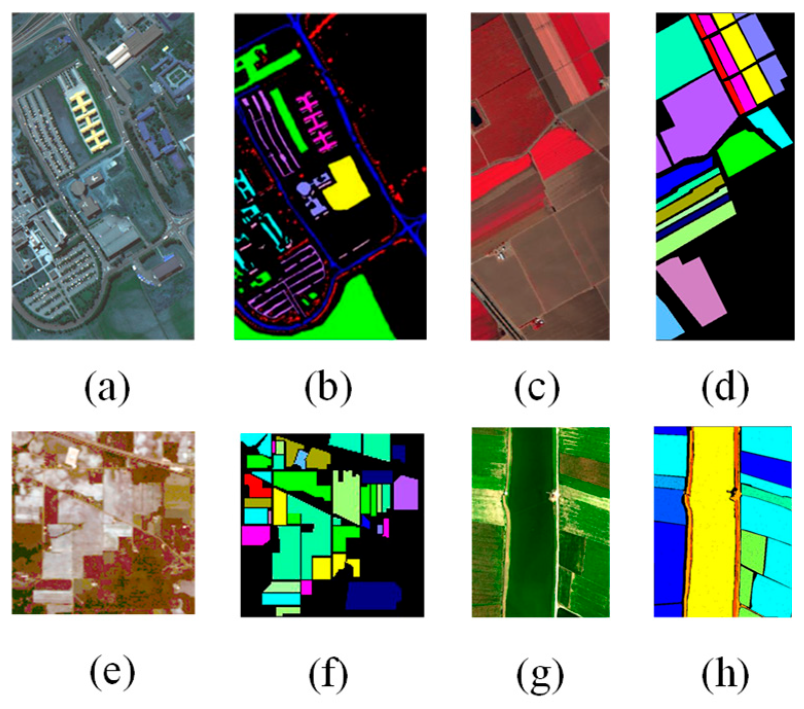
The proposed model was evaluated using four benchmark HSI datasets: Pavia University (PU), Salinas (SA), Indian Pines (IP), and Longkou. Representing distinct geographical environments and diverse object categories, this selection enables a comprehensive test of the model’s generalization ability. False-color (FC) imagery and corresponding ground-truth (GT) maps for all datasets appear in Figure 3. The specific details of each dataset are depicted in Table 1, Table 2, Table 3 and Table 4.
Pavia University (PU): Acquired by the ROSIS-03 sensor over the University of Pavia, Italy, in 2001, the PU dataset has a spatial resolution of 1.3 m and spatial dimensions of 610 × 340 pixels. It originally contained 115 spectral bands ranging from 0.43 to 0.86 µm; after removing 12 noisy bands, 103 bands were retained for experiments. The dataset includes nine ground-truth classes.
Salinas (SA): The Salinas dataset has a spatial resolution of roughly 3.7 m and a spatial scope of 512 × 217 pixels. It features 224 spectral channels from 400 to 2500 nm. However, only 204 bands are used due to water vapor absorption. The dataset has 16 agricultural land-cover classes.
Indian Pines (IP): The Indian Pines dataset was gathered in 1992 via the AVIRIS sensor. It has a spatial resolution of approximately 20 m and a spatial extent of 145 × 145 pixels. Initially, it had 224 spectral bands. However, 20 water-absorption bands and four zero bands were eliminated, leaving 200 bands for experiments. The dataset encompasses 16 classes.
LongKou: The WHU-Hi LongKou dataset was gathered on 17 July 2018 over Longkou town in Hubei Province, China. It was collected by a Headwall Nano-Hyperspec sensor mounted on a drone. The dataset has a spatial size of 550 × 400 pixels and a spatial resolution of roughly 0.463 m. It consists of 270 spectral channels spanning 400–1000 nm. There are nine land-cover types in this area.
Both the ImageNet and HSI training iterations were set to 1000. To rigorously simulate an extreme data regime, we set K = 1 (only one labeled sample per class) and N = 19 for each training episode to ensure that every episode maintained a balanced, 19-way evaluation across all datasets. C is determined by the number of classes in the HSI dataset. During the experiments, five labeled samples from each class of the HSI dataset were randomly picked as the training set, while the remaining samples served as the test set. For few-shot learning methods, 200 labeled samples per class were randomly chosen. In addition, to eliminate the impact of random sampling, all experiments were carried out ten times. Our model was optimized with Adam, and the learning rate was set to 0.001. The overall accuracy ( O A ), average accuracy ( A A ), and kappa coefficient ( κ ) were used to evaluate the classification performance of all methods.

3.2. Ablation Experiments

3.2.1. Combination of Different Modules

To evaluate the transfer spatial feature extraction module (SpaM) and spectral residual feature extraction module (SpeM) in few-shot HSI tasks, four schemes were tested across four datasets. The overall accuracies (OAs) for each scheme are presented in Table 5, with the best results highlighted in bold. The table includes the “SpaM-Scratch” configuration, in which the spatial module is trained from scratch on HSI data, thereby providing a direct assessment of the benefit gained from ImageNet pre-training. Compared with “SpaM-Scratch”, the ImageNet-pre-trained SpaM yields statistically significant OA improvements of 3.3–4.1%, confirming the value of transfer learning. When used individually, SpaM consistently outperforms SpeM, indicating that the pre-trained spatial features remain more informative than spectral features learned from extremely few samples. Combining the pre-trained SpaM with SpeM achieves the highest OA on every dataset, demonstrating that the fusion of complementary spatial and spectral representations yields the most comprehensive feature set for few-shot HSI classification.

3.2.2. SAM Contribution Analysis

To verify the impact of the SAM, the proposal was trained with and without the SAM under the standard five-shot setting (five samples per class). All other modules and hyperparameters were kept identical. Table 6 reports the average results over 10 independent runs. As shown in Table 6, the SAM brings significant performance improvements in all four benchmark datasets, with the largest improvements (+3.58%) in the Indian Pines dataset, which has the most complex spatial structure. This phenomenon can be attributed to the dual-path pooling mechanism of the SAM: the maximum pooling branch effectively captures the irregular boundary characteristics of farmland patches in this dataset, while the average pooling branch maintains spectral consistency in homogeneous crop areas. It is worth noting that although the introduction of the SAM results in a slight increase in the model standard deviation (Pavia University: ±1.56 vs. ±0.4), its classification accuracy in boundary-sensitive areas has significantly improved (such as the “Gravel” class F1 value, which increased by 9.2%), which verifies the robustness enhancement effect of the module in spatial heterogeneous scenarios.

3.2.3. Loss Function

The loss function within our proposed methodology is paramount in improving the classification accuracy. The loss strategy amalgamates cross-entropy with contrastive supervision to learn domain-agnostic feature representations. This fusion is designed to capitalize on the strengths of both components: the discriminative power of cross-entropy and the distinctive feature separation afforded by contrastive learning.
To validate the impact of the proposed loss strategy, all other model components are maintained constant while varying the loss function employed. As depicted in Table 7, the empirical results offer a comparative analysis of the performance across four distinct datasets. They reveal that the incorporation of supervised contrastive learning significantly outperforms the reliance on cross-entropy loss in isolation. This demonstrates that the mechanism of contrastive learning introduces an enhanced capacity for the model to discern between classes. Moreover, the amalgamated loss function, which incorporates both the cross-entropy and contrastive loss, emerges as the most effective, which demonstrates the superiority of our proposed strategy.

3.3. Comparison with State-of-the-Art Algorithms

In this experiment, several state-of-the-art algorithms were employed for comparison, including the supervised machine learning method SVM [14], the 3D conv-based method SSRN [22], the data augmentation method RODA [24], a heterogeneous transfer learning network (HTLN) [36], the few-shot learning methods DFSL [23] and S3Net [49], deep cross-domain few-shot learning for hyperspectral image classification (DCLN) [47], and enhancing a contrastive learning with positive pair mining network (CPPM) [54] to verify the validity of the proposed method. Applying uniform evaluation criteria for SVM, five randomly selected labeled samples per class served as training data. All benchmark methods underwent identical training–validation–testing procedures on consistent datasets.

3.3.1. The Quantitative Evaluations

The detailed classification evaluations presented in Table 8, Table 9, Table 10 and Table 11 provide a comprehensive assessment of the performance of various models across four distinct datasets. A meticulous analysis of these data reveals that SVM performs worst in extremely small sample sizes, demonstrating the bottleneck of shallow models in learning high-dimensional spectral features. While the data augmentation method RODA outperforms SVM, its performance fluctuates significantly, reflecting the noise sensitivity of the generated samples. This contradicts the stringent spectral fidelity requirements of HSIs. The 3D-CNN architecture SSRN performs well with sufficient samples but degrades significantly in the five-shot setting, highlighting the dependence of convolutional networks on data size. The small sample-specific models DFSL, S3Net, and CPPM optimize feature embedding through meta-learning and self-supervised learning and perform well on the PU and SA datasets, but their performance drops sharply for the IP dataset, indicating that spectral–spatial correlation modeling in complex farmland scenes is still insufficient. Empirical evaluations show that HTLN delivers competitive performance relative to few-shot learning methods on multiple datasets, confirming transfer learning’s capability to address data scarcity challenges. Notably, our method delivers competitive accuracy across diverse datasets in classes C1, C2, and C8 on the Pavia University (PU) dataset. On the Salinas dataset, our method yields satisfactory classification outcomes for nearly all classes, which is attributed to the ability of the residual spectral network to extract narrowband features and the multi-scale fusion of the SAM. Furthermore, our proposal secures the highest results among the seven classes in the Indian Pines (IP) dataset. In the Longkou dataset, which boasts a higher spatial resolution, the performance of all models is observed to improve. The overall performance metrics of our method are also found to be superior, with the highest OA, AA, and κ values across the four datasets. These findings suggest that our proposed method offers a robust strategy for enhancing model performance in few-shot scenarios.

3.3.2. The Qualitative Evaluations

The visual classification maps generated by a variety of methods across the four datasets are depicted in Figure 4, Figure 5, Figure 6 and Figure 7. A comparative analysis reveals that few-shot methods, including DFSL, S3Net, DCLN, and our proposed approach, yield purer and smoother classification maps compared to other methodologies. The SVM classification maps exhibit numerous speckles across many regions and display relatively blurred boundaries between different categories, indicating that SVM, with its simplistic structure, performs poorly when confronted with small sample challenges. While the RODA classification maps are comparatively clearer than those of SVM, they remain less than satisfactory. This observation suggests that data augmentation strategies can partially mitigate the impact of the small sample crisis. However, since the information primarily derives from limited labeled samples, model stability is susceptible to the influence of randomly sampled training data. The SSRN classification maps demonstrate poor results, potentially due to constraints in data volume. Although the classification maps from the few-shot models are not without imperfections, the results are deemed acceptable given the scarcity of training samples. For the Pavia University dataset, our proposed method accurately identifies almost all pixels in the “Gravel,” “Metal-sheets,” “Bare-soil,” and “Bitumen” (C3, C5, C6, and C7) categories. Their boundary clarity is significantly better than that of SVM and SSRN, reflecting the strong representation power of the migrated spatial features on heterogeneous objects. CPPM’s misjudgment of the “Bare-soil” class (C6) reveals the limitations of simple contrastive learning for spectral confusion scenes, while DTCLN corrects such errors through spectral residuals. The “Lettuce” classes (C11–C14) in Salinas show large areas of confusion in S3Net, while DTCLN maintains 98.20% accuracy, thanks to the noise injection of the spectral enhancement module that improves the model’s robustness to band shifts. With only 200 samples in the IP “Wheat” class (C13), DTCLN still achieves 99.14% accuracy, proving that under the hybrid loss constraint, the model avoids overfitting to the minority class.
Overall, when compared to other few-shot methods, our proposed model achieves acceptable classification maps that closely resemble the corresponding ground-truth images across the four datasets. This performance improvement stems from our proposed model’s enhanced ability to learn discriminative spectral–spatial features from limited samples. This capability is achieved by leveraging a transferred spatial model pre-trained on large datasets and incorporating a specially designed spectral residual network.

3.4. Effect of the Labeled Samples

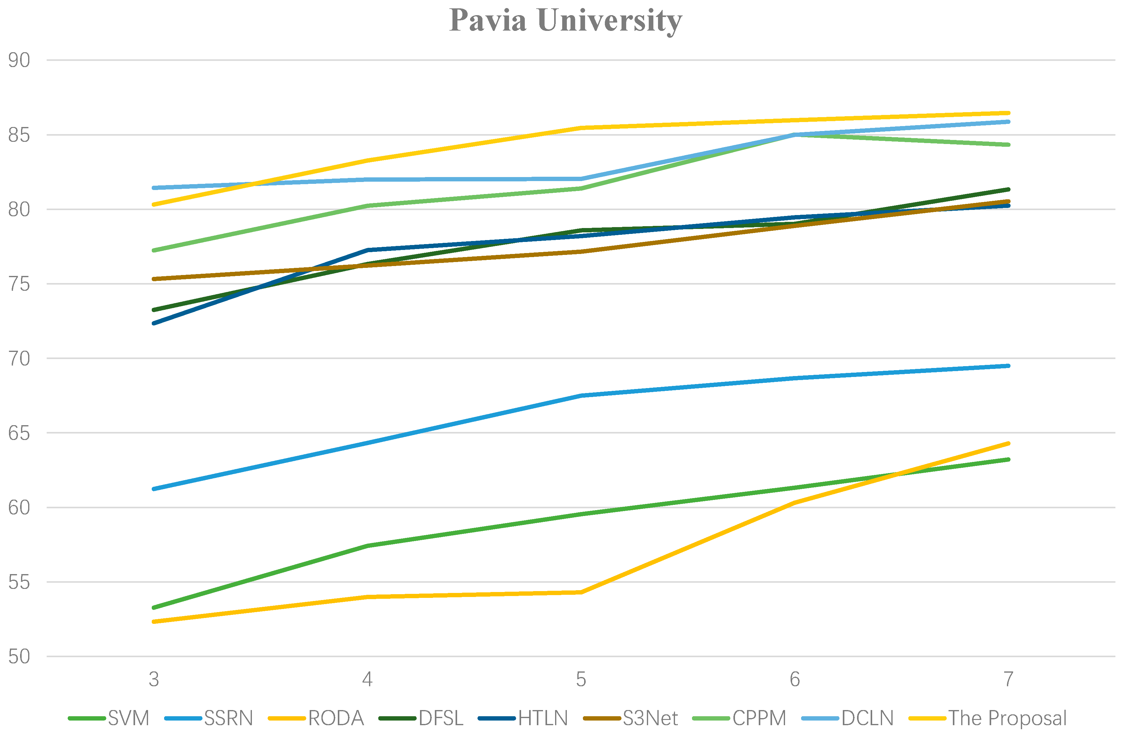
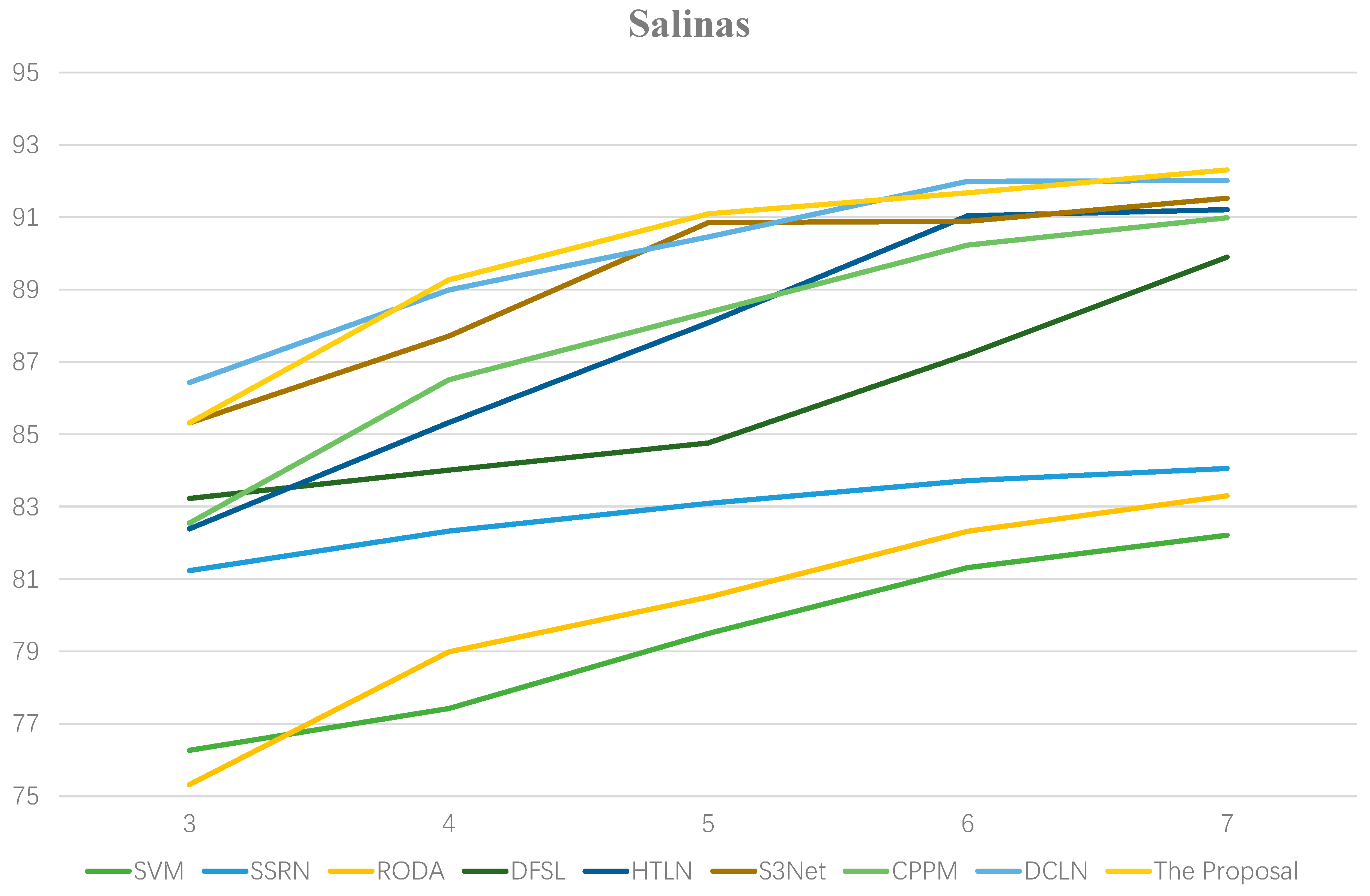
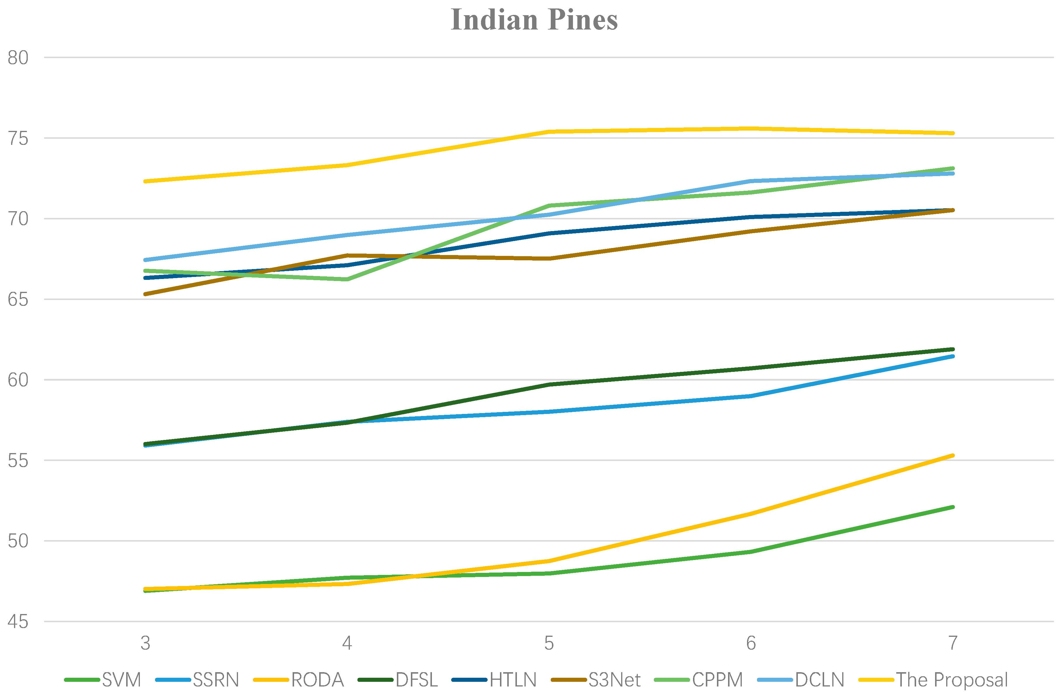
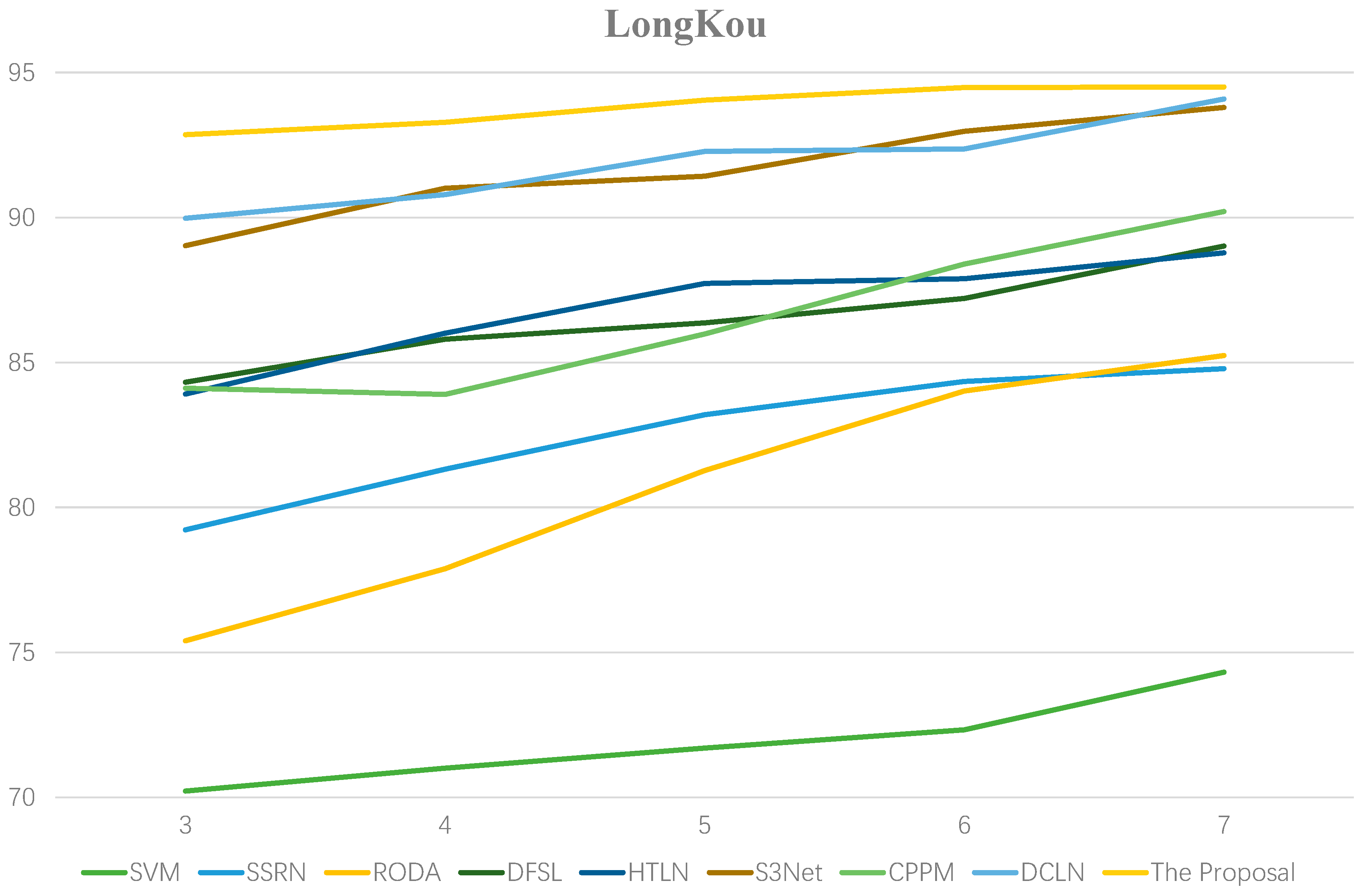
To explore the model’s generalization capabilities with very few labeled samples, we conducted supplementary experiments in settings with 3–7 samples/class. As shown in Figure 8, Figure 9, Figure 10 and Figure 11, the OAs of all methods show a steady upward trend with increasing number of available labels, consistent with the common belief that richer samples lead to better performance. Within this range, our method achieves relatively high OAs in most cases, demonstrating its good adaptability to changes in sample size. Furthermore, even with the most scarce samples (three/class), the OA remains competitive, suggesting the potential advantages of the proposed strategy in extremely low-sample scenarios.

3.5. Analysis of Computational Complexity

The experimental results, shown in Table 12, clearly reveal the differences between different methods in training time, testing time, and parameter count. Traditional SVMs once again dominate with seconds-long training times and minimal parameter counts. All deep learning approaches, however, incur significant time overheads due to their network architecture and backpropagation. SSRN and RODA, due to their efficient feature extraction and sample augmentation, maintain training times of 400–1300 s on all four datasets, with parameter counts below 0.4M, resulting in the lowest overall training burden. DFSL and S3Net, utilizing a minimalist framework, further reduce trainable parameters to 0.03–0.09 M, while maintaining test latency under 7 s, demonstrating the advantages of their lightweight design. In contrast, HTLN, CPPM, and DCLN, due to the introduction of cross-domain alignment or positive sample mining modules, see their parameter counts rise to 0.63–0.85 M. This results in training times generally exceeding 1400 s, with test latency reaching as high as nearly 25 s, representing computational bottlenecks. The method proposed in this paper maintains fewer trainable parameters (compared with HTLN/DCLN/CPPM) while keeping the training and testing times within an acceptable range, indicating that it achieves a better balance between computational efficiency and classification performance.

4. Conclusions

In this work, a deep transfer contrastive learning network is proposed for few-shot HSI classification tasks. To mitigate sample scarcity, a spectral data augmentation method using random spectral shifting and noise injection improves the model’s robustness to real-world perturbations. Subsequently, transfer learning is incorporated into the proposed spatial–spectral feature extraction network. The combination of an ImageNet-pretrained spatial feature extraction module and a spectral residual network significantly improves feature representation capabilities. The SAM captures multi-scale context through dual-path pooling (maximum pooling and average pooling), which significantly improves boundary-sensitive areas. Concurrently, the hybrid loss function explicitly expands inter-class distances and compresses intra-class radii, directly alleviating the high inter-class similarity and large intra-class variance issues of HSIs. Experimental results on four public HSI datasets demonstrate that our method achieves competitive performance even with limited training samples. However, the method is still limited by computational complexity and generalization ability in extreme scenarios (such as low-resolution HSIs). In the future, lightweight deployment and cross-sensor generalization optimization need to be explored.

Author Contributions

Conceptualization, G.Y. and Z.W.; methodology, G.Y.; software, G.Y.; validation, G.Y. and Z.W.; formal analysis, G.Y. and Z.W.; investigation, G.Y.; resources, G.Y.; data curation, G.Y.; writing—original draft preparation, G.Y.; writing—review and editing, G.Y. and Z.W.; visualization, G.Y. and Z.W.; supervision, Z.W.; project administration, Z.W.; funding acquisition, Z.W. All authors have read and agreed to the published version of the manuscript.

Funding

This work was supported by the Hainan Key Research and Development Plan for Scientific and Technological Collaboration Projects under Grant GHYF2022015-Research on Medical Imaging Aided Diagnosis of Infant Brain Development Diseases.

Data Availability Statement

The original contributions presented in this study are included in the article and were derived from the following resources available in the public domain: Public HSI dataset at https://www.ehu.eus/ccwintco/index.php?title=Hyperspectral_Remote_Sensing_Scenes (accessed on 1 December 2024).

Conflicts of Interest

The authors declare no conflict of interest.

References

  1. Lu, B.; Dao, P.D.; Liu, J.; He, Y.; Shang, J. Recent advances of hyperspectral imaging technology and applications in agriculture. Remote Sens. 2020, 12, 2659. [Google Scholar] [CrossRef]
  2. Li, Y.; Wang, T.; Cao, Z.; Xin, H.; Wang, R. Efficient Unsupervised Clustering of Hyperspectral Images via Flexible Multi-Anchor Graphs. Remote Sens. 2025, 17, 2647. [Google Scholar] [CrossRef]
  3. Peng, J.; Sun, W.; Li, W.; Li, H.-C.; Meng, X.; Ge, C.; Du, Q. Low-rank and sparse representation for hyperspectral image processing: A review. IEEE Geosci. Remote Sens. Mag. 2022, 10, 10–43. [Google Scholar] [CrossRef]
  4. Li, N.; Wang, Z.; Cheikh, F.A. Discriminating spectral–spatial feature extraction for hyperspectral image classification: A review. Sensors 2024, 24, 2987. [Google Scholar] [CrossRef]
  5. Liu, J.; Feng, Q.; Liang, T.; Yin, J.; Gao, J.; Ge, J.; Hou, M.; Wu, C.; Li, W. Estimating the forage neutral detergent fiber content of alpine grassland in the Tibetan Plateau using hyperspectral data and machine learning algorithms. IEEE Trans. Geosci. Remote Sens. 2022, 60, 4405017. [Google Scholar] [CrossRef]
  6. Anand, R.; Veni, S.; Araint, J. Big data challenges in airborne hyperspectral image for urban landuse classification. In Proceedings of the 2017 International Conference on Advances in Computing, Communications and Informatics (ICACCI), Udupi, India, 13–16 September 2017; pp. 1808–1814. [Google Scholar]
  7. Yang, X.; Yu, Y. Estimating soil salinity under various moisture conditions: An experimental study. IEEE Trans. Geosci. Remote Sens. 2017, 55, 2525–2533. [Google Scholar] [CrossRef]
  8. Yang, G.; Wang, Z. Self-supervised contrastive learning residual network for hyperspectral image classification under limited labeled samples. In Proceedings of the 2024 7th International Conference on Image and Graphics Processing, Beijing, China, 19–21 January 2024; pp. 116–121. [Google Scholar]
  9. Démoulin, R.; Gastellu-Etchegorry, J.-P.; Briottet, X.; Marionneau, M.; Zhen, Z.; Adeline, K.; Dantec, V.L. Hyperspectral Remote Sensing and 3D Radiative Transfer Modelling for Maize Crop Monitoring. In Proceedings of the 13th EARSeL Workshop on Imaging Spectroscopy, Valence, Spain, 24–26 April 2024. [Google Scholar]
  10. Dalal, N.; Triggs, B. Histograms of oriented gradients for human detection. In Proceedings of the Computer Vision and Pattern Recognition, San Diego, CA, USA, 20–26 June 2005; Volime 1, pp. 886–893. [Google Scholar]
  11. Abdi, H.; Williams, L.J. Principal component analysis. Wiley Interdiscip. Rev. Comput. Stat. 2010, 2, 433–459. [Google Scholar] [CrossRef]
  12. Li, W.; Chen, C.; Su, H.; Du, Q. Local binary patterns and extreme learning machine for hyperspectral imagery classification. IEEE Trans. Geosci. Remote Sens. 2015, 53, 3681–3693. [Google Scholar] [CrossRef]
  13. Zhang, Y.; Cao, G.; Li, X.; Wang, B. Cascaded random forest for hyperspectral image classification. IEEE J. Sel. Topics Appl. Earth Observ. Remote Sens. 2018, 11, 1082–1094. [Google Scholar] [CrossRef]
  14. Melgani, F.; Bruzzone, L. Classification of hyperspectral remote sensing images with support vector machines. IEEE Trans. Geosci. Remote Sens. 2004, 42, 1778–1790. [Google Scholar] [CrossRef]
  15. Ma, L.; Crawford, M.M.; Tian, J. Local manifold learning-based k-nearest-neighbor for hyperspectral image classification. IEEE Trans. Geosci. Remote Sens. 2010, 48, 4099–4109. [Google Scholar] [CrossRef]
  16. Wang, X. Hyperspectral image classification powered by Khatri-Rao decomposition-based multinomial logistic regression. IEEE Trans. Geosci. Remote Sens. 2022, 60, 5530015. [Google Scholar] [CrossRef]
  17. Maffei, A.; Haut, J.M.; Paoletti, M.E.; Plaza, J.; Bruzzone, L.; Plaza, A. A single model CNN for hyperspectral image denoising. IEEE Trans. Geosci. Remote Sens. 2020, 58, 2516–2529. [Google Scholar] [CrossRef]
  18. Tao, C.; Pan, H.; Li, Y.; Zou, Z. Unsupervised spectral-spatial feature learning with stacked sparse autoencoder for hyperspectral imagery classification. IEEE Geosci. Remote Sens. Lett. 2015, 12, 2438–2442. [Google Scholar] [CrossRef]
  19. Li, C.; Wang, Y.; Zhang, X.; Gao, H.; Yang, Y.; Wang, J. Deep belief network for spectral–spatial classification of hyperspectral remote sensor data. Sensors 2019, 19, 204. [Google Scholar] [CrossRef] [PubMed]
  20. Audebert, N.; Le Saux, B.; Lefèvre, S. Deep learning for classification of hyperspectral data: A comparative review. IEEE Geosci. Remote Sens. Mag. 2019, 7, 159–173. [Google Scholar] [CrossRef]
  21. Li, Y.; Zhang, H.; Shen, Q. Spectral-spatial classification of hyperspectral imagery with 3D convolutional neural network. Remote Sens. 2017, 9, 67. [Google Scholar] [CrossRef]
  22. Zhong, Z.; Li, J.; Luo, Z.; Chapman, M. Spectral-spatial residual network for hyperspectral image classification: A 3-D deep learning framework. IEEE Trans. Geosci. Remote Sens. 2018, 56, 847–858. [Google Scholar] [CrossRef]
  23. Liu, B.; Yu, X.; Yu, A.; Zhang, P.; Wan, G.; Wang, R. Deep few-shot learning for hyperspectral image classification. IEEE Trans. Geosci. Remote Sens. 2019, 57, 2290–2304. [Google Scholar] [CrossRef]
  24. Haut, J.M.; Paoletti, M.E.; Plaza, J.; Plaza, A.; Li, J. Hyperspectral image classification using random occlusion data augmentation. IEEE Geosci. Remote Sens. Lett. 2019, 16, 1751–1755. [Google Scholar] [CrossRef]
  25. Zhu, L.; Chen, Y.; Ghamisi, P.; Benediktsson, J.A. Generative adversarial networks for hyperspectral image classification. IEEE Trans. Geosci. Remote Sens. 2018, 56, 5046–5063. [Google Scholar] [CrossRef]
  26. Aburaed, N.; Alkhatib, M.Q.; Marshall, S.; Zabalza, J.; Al Ahmad, H. Hyperspectral data scarcity problem from a super resolution perspective: Data augmentation analysis and scheme. In Proceedings of the IEEE International Geoscience and Remote Sensing Symposium, Pasadena, CA, USA, 16–21 July 2023; pp. 5056–5057. [Google Scholar]
  27. Liu, S.; Li, H.; Jiang, C.; Feng, J. Spectral–spatial graph convolutional network with dynamic-synchronized multiscale features for few-shot hyperspectral image classification. Remote Sens. 2024, 16, 895. [Google Scholar] [CrossRef]
  28. Shi, M.; Ren, J. A lightweight dense relation network with attention for hyperspectral image few-shot classification. Eng. Appl. Artif. Intell. 2023, 126, 106842. [Google Scholar] [CrossRef]
  29. Zhang, Z.; Gao, D.; Liu, D. Spectral-spatial domain attention network for hyperspectral image few-shot classification. Remote Sens. 2024, 16, 592. [Google Scholar] [CrossRef]
  30. Jiang, S.; Jia, S. A 3D lightweight Siamese network for hyperspectral image classification with limited samples. In Proceedings of the 10th International Conference on Computing and Pattern Recognition, Shanghai, China, 15–17 October 2021; pp. 142–148. [Google Scholar]
  31. Gao, K.; Liu, B.; Yu, X.; Zhang, P.; Tan, X.; Sun, Y. Small sample classification of hyperspectral image using model-agnostic meta-learning algorithm and convolutional neural network. Int. J. Remote Sens. 2020, 42, 3090–3122. [Google Scholar] [CrossRef]
  32. Zhou, F.; Zhang, L.; Wei, W.; Bai, Z.; Zhang, Y. Meta transfer learning for few-shot hyperspectral image classification. In Proceedings of the IEEE International Geoscience and Remote Sensing Symposium, Brussels, Belgium, 11–16 July 2021; pp. 3681–3684. [Google Scholar]
  33. Gao, K.; Liu, B.; Yu, X.; Yu, A. Unsupervised meta learning with multiview constraints for hyperspectral image small sample set classification. IEEE Trans. Image Process. 2022, 31, 3449–3462. [Google Scholar] [CrossRef]
  34. Zhao, L.; Luo, W.; Liao, Q.; Chen, S.; Wu, J. Hyperspectral image classification with contrastive self-supervised learning under limited labeled samples. IEEE Geosci. Remote Sens. Lett. 2022, 19, 6008205. [Google Scholar] [CrossRef]
  35. Qu, Y.; Baghbaderani, R.K.; Qi, H. Few-shot hyperspectral image classification through multitask transfer learning. In Proceedings of the 2019 10th Workshop on Hyperspectral Imaging and Signal Processing: Evolution in Remote Sensing (WHISPERS), Amsterdam, The Netherlands, 24–26 September 2019; pp. 1–5. [Google Scholar]
  36. He, X.; Chen, Y.; Ghamisi, P. Heterogeneous transfer learning for hyperspectral image classification based on convolutional neural network. IEEE Trans. Geosci. Remote Sens. 2020, 58, 3246–3263. [Google Scholar] [CrossRef]
  37. Li, X.; Cao, Z.; Zhao, L.; Jiang, J. ALPN: Active-learning-based prototypical network for few-shot hyperspectral imagery classification. IEEE Geosci. Remote Sens. Lett. 2022, 19, 5508305. [Google Scholar] [CrossRef]
  38. Thoreau, R.; Achard, V.; Risser, L.; Berthelot, B.; Briottet, X. Active learning for hyperspectral image classification: A comparative review. IEEE Geosci. Remote Sens. Mag. 2022, 10, 256–278. [Google Scholar] [CrossRef]
  39. Zhang, S.; Chen, Z.; Wang, D.; Wang, Z.J. Cross-domain few-shot contrastive learning for hyperspectral images classification. IEEE Geosci. Remote Sens. Lett. 2022, 19, 5514505. [Google Scholar] [CrossRef]
  40. Liu, Q.; Peng, J.; Zhang, G.; Sun, W.; Du, Q. Deep contrastive learning network for small-sample hyperspectral image classification. J. Remote Sens. 2023, 3, 0025. [Google Scholar] [CrossRef]
  41. Liu, Q.; Peng, J.; Chen, N.; Sun, W.; Du, Q.; Zhou, Y. Refined prototypical contrastive learning for few-shot hyperspectral image classification. IEEE Trans. Geosci. Remote Sens. 2023, 61, 5506214. [Google Scholar] [CrossRef]
  42. Jaiswal, A.; Babu, A.R.; Zadeh, M.Z.; Banerjee, D.; Makedon, F. A survey on contrastive self-supervised learning. Technologies 2020, 9, 2. [Google Scholar] [CrossRef]
  43. Devabathini, N.J.; Mathivanan, P. Sign language recognition through video frame feature extraction using transfer learning and neural networks. In Proceedings of the 2023 International Conference on Next Generation Electronics (NEleX), Vellore, India, 14–16 December 2023; pp. 1–6. [Google Scholar]
  44. Dhillon, G.S.; Chaudhari, P.; Ravichandran, A.; Soatto, S. A baseline for few-shot image classification. arXiv 2019, arXiv:1909.02729. [Google Scholar]
  45. Settles, B. Active Learning Literature Survey; University of Wisconsin-Madison: Madison, WI, USA, 2009. [Google Scholar]
  46. Li, Z.; Liu, M.; Chen, Y.; Xu, Y.; Li, W.; Du, Q. Deep cross-domain few-shot learning for hyperspectral image classification. IEEE Trans. Geosci. Remote Sens. 2022, 60, 5501618. [Google Scholar] [CrossRef]
  47. Pan, S.J.; Yang, Q. A survey on transfer learning. IEEE Trans. Knowl. Data Eng. 2009, 22, 1359. [Google Scholar] [CrossRef]
  48. Xue, Z.; Zhou, Y.; Du, P. S3Net: Spectral–spatial Siamese network for few-shot hyperspectral image classification. IEEE Trans. Geosci. Remote Sens. 2022, 60, 5531219. [Google Scholar] [CrossRef]
  49. Theckedath, D.; Sedamkar, R.R. Detecting affect states using VGG16, ResNet50 and SE-ResNet50 networks. SN Comput. Sci. 2020, 1, 79. [Google Scholar] [CrossRef]
  50. Elsayed, G.; Krishnan, D.; Mobahi, H.; Regan, K.; Bengio, S. Large margin deep networks for classification. In Proceedings of the Advances in Neural Information Processing Systems, Montreal, Canada, 3–8 December 2018; pp. 850–860. [Google Scholar]
  51. Song, L.; Feng, Z.; Yang, S.; Zhang, X.; Jiao, L. Self-supervised assisted semi-supervised residual network for hyperspectral image classification. Remote Sens. 2022, 14, 2997. [Google Scholar] [CrossRef]
  52. Yang, H.; Ni, J.; Gao, J.; Han, Z.; Luan, T. A novel method for peanut variety identification and classification by improved VGG16. Sci. Rep. 2021, 11, 15756. [Google Scholar] [CrossRef] [PubMed]
  53. Chen, T.; Kornblith, S.; Norouzi, M.; Hinton, G. A Simple Framework for Contrastive Learning of Visual Representations. In Proceedings of the Machine Learning Research (PMLR), Virtual Event, 13–18 July 2020; Volume 119, pp. 1597–1607. [Google Scholar]
  54. Braham, N.A.A.; Mairal, J.; Chanussot, J.; Mou, L.; Zhu, X.X. Enhancing contrastive learning with positive pair mining for few-shot hyperspectral image classification. IEEE J. Sel. Topics Appl. Earth Observ. Remote Sens. 2024, 17, 8509–8526. [Google Scholar] [CrossRef]
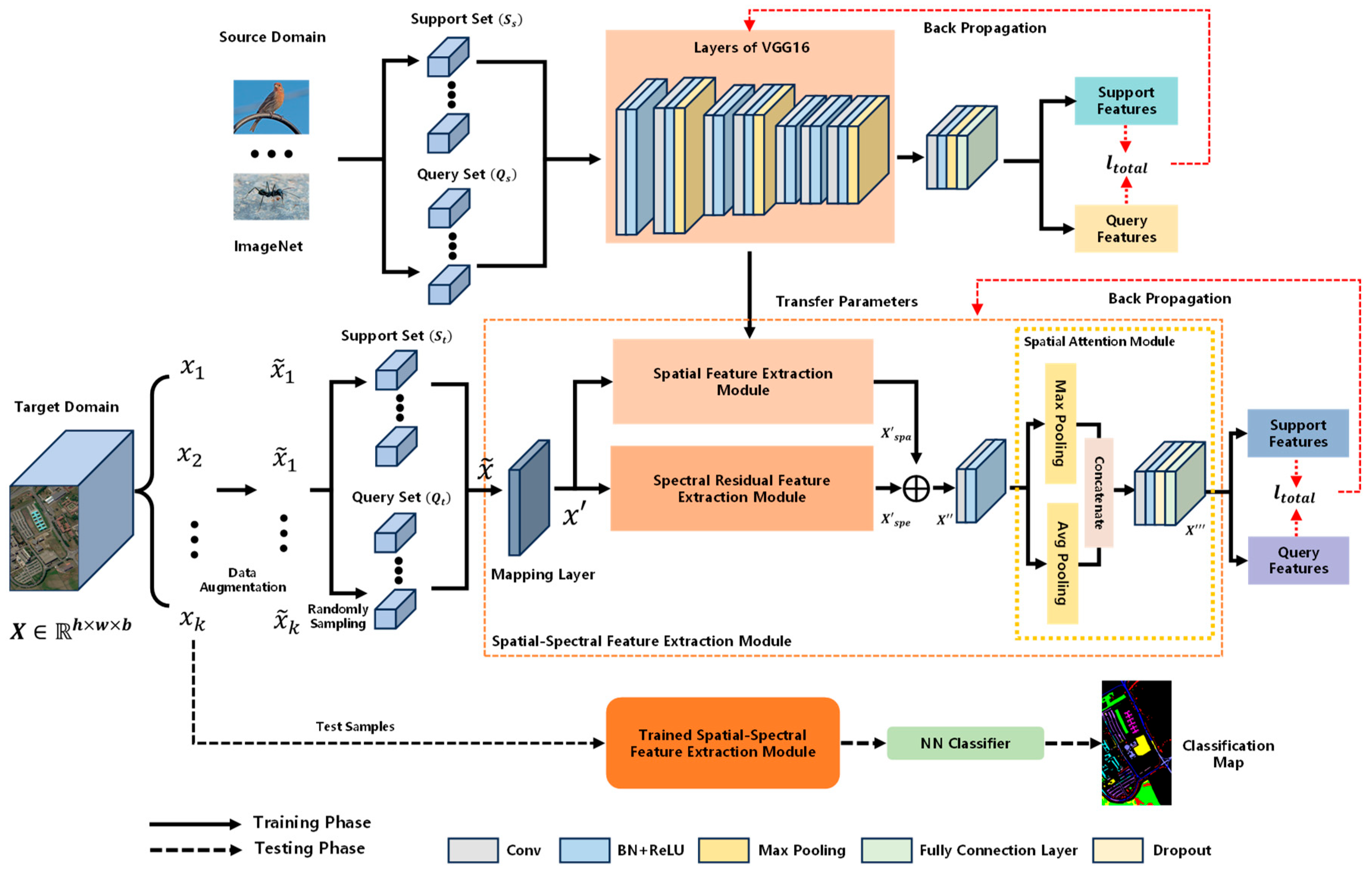
Figure 1. Flowchart of the proposed network.
Remotesensing 17 02800 g001
Figure 2. Framework of the proposed spectral residual feature module.
Remotesensing 17 02800 g002
Figure 3. The false-color images and ground-truth maps. (a,b): Pavia University. (c,d): Salinas. (e,f): Indian Pines. (g,h): LongKou.
Remotesensing 17 02800 g003
Figure 4. Classification maps for different methods using the PU dataset.
Remotesensing 17 02800 g004
Figure 5. Classification maps for different methods using the Salinas dataset.
Remotesensing 17 02800 g005
Figure 6. Classification maps for different methods using the IP dataset.
Remotesensing 17 02800 g006
Figure 7. Classification maps for different methods using the LongKou dataset.
Remotesensing 17 02800 g007
Figure 8. Classification accuracies (%) generated by different numbers of labeled samples from the PU dataset.
Remotesensing 17 02800 g008
Figure 9. Classification accuracies (%) generated by different numbers of labeled samples from the Salinas dataset.
Remotesensing 17 02800 g009
Figure 10. Classification accuracies (%) generated by different numbers of labeled samples from the IP dataset.
Remotesensing 17 02800 g010
Figure 11. Classification accuracies (%) generated by different numbers of labeled samples from the LongKou dataset.
Remotesensing 17 02800 g011
Table 1. Samples from the Pavia University dataset.
Pavia University
No.Land-Cover TypeTrainingTest
1Asphalt56626
2Medows518,644
3Gravel52094
4Trees53059
5Metal-sheets51340
6Bare-soil55024
7Bitumen51325
8Bricks53677
9Shadows5942
Total4542,731
Table 2. Samples from the Salinas University dataset.
Salinas
No.Land-Cover TypeTrainingTest
1Brocoli 152004
2Brocoli 253721
3Fallow51971
4Fallow_plow51389
5Fallow_smooth52673
6Stubble53954
7Celery53574
8Grapes_untrained511,266
9Soil56198
10Corn53273
11Lettuce_4_wk51063
12Lettuce_5_wk51922
13Lettuce_6_wk5911
14Lettuce_7_wk51065
15Vinyard-untrained57263
16Vinyard-vertical51802
Total8054,049
Table 3. Samples from the Indian Pines University dataset.
Indian Pines
No.Land-Cover TypeTrainingTest
1Alfalfa541
2Corn-notill51432
3Corn-mintill5825
4Corn5232
5Grass-pasture5478
6Grass-trees5725
7Grass-pasture mowed523
8Hay-windrowed5473
9Oats515
10Soybean-notill5967
11Soybean-mintill52450
12Soybean-clean5588
13Wheat5200
14Woods51260
15Buildings-grass5381
16Stone-steel588
Total8010,169
Table 4. Samples from the LongKou University dataset.
LongKou
No.Land-Cover TypeTrainingTest
1Corn534,506
2Cotton58369
3Sesame53026
4Broad-leaf soy-bean563,207
5Narrow-leaf soybean54146
6Rice511,849
7Water567,051
8Roads and Houses57119
9Mixed weed55224
Total45204,497
Table 5. OAs of different schemes for the four datasets.
DatasetSchemesOA (%)
Pavia UniversitySpaM (Pre-trained) 82.24 ± 1.48
SpaM (Scratch) 78.12 ± 2.05
SpeM 81.71 ± 1.22
SpaM (Pre-trained) + SpeM 85.46 ± 1.56
SalinasSpaM (Pre-trained) 89.43 ± 0.83
SpaM (Scratch) 86.71 ± 1.36
SpeM 87.91 ± 0.99
SpaM (Pre-trained) + SpeM 91.10 ± 2.32
Indian PinesSpaM (Pre-trained) 74.59 ± 2.10
SpaM (Scratch) 71.05 ± 2.44
SpeM 73.86 ± 1.73
SpaM (Pre-trained) + SpeM 75.40 ± 2.21
LongKouSpaM (Pre-trained) 91.51 ± 1.82
SpaM (Scratch) 89.20 ± 1.68
SpeM 90.79 ± 1.10
SpaM (Pre-trained) + SpeM 94.05 ± 1.37
Table 6. Influence of the spatial attention module (SAM) on overall accuracy (OA%).
DatasetWith SAMWithout SAM∆OA (%)
Pavia University 85.46 ± 1.56 82.11   ±   0.4 + 3.35
Salinas 91.10 ± 2.32 88.96   ±   0.3 + 2.14
Indian Pines 75.40 ± 2.21 71.82   ±   0.6 + 3.58
LongKou 94.05 ± 1.37 91.74   ±   0.3 +2.31
Table 7. Ablation studies on the loss function.
DatasetLoss FunctionOA (%)
Pavia University L C E 84.73 ± 2.47
L c o n 85.21 ± 1.12
L C E   +   L c o n 85.46 ± 1.56
Salinas L C E 90.73 ± 1.49
L c o n 90.13 ± 1.76
L C E   +   L c o n 91.10 ± 2.32
Indian Pines L C E 73.79 ± 0.97
L c o n 74.34 ± 1.33
L C E   +   L c o n 75.40 ± 2.21
LongKou L C E 89.97 ± 1.72
L c o n 91.39 ± 1.62
L C E   +   L c o n 94.05 ± 1.37
Table 8. Classification results from different models for the Pavia University dataset.
SVMSSRNRODADFSLHTLNS3NetCPPMDCLNOurs
172.4276.9935.5398.2489.7781.7679.1273.8683.21
282.6963.9751.8098.4574.3775.5185.4861.7791.14
340.7155.9884.7848.0462.8770.0863.1339.8980.47
467.9091.8286.7750.9494.6985.8392.0794.3492.54
599.9999.5110099.9299.8699.9399.7298.7998.48
627.8363.2949.7877.9657.7964.1771.0786.0570.34
741.8955.6794.7273.5393.1295.1479.1790.7689.60
854.8445.8520.4484.2481.3572.4569.9763.9174.43
981.7599.6396.8275.6898.0694.9097.6098.9799.18
OA59.54
±2.38
67.49
±1.27
54.30
±1.03
78.58
±2.77
78.20
±0.98
77.15
±1.11
81.39
±2.93
82.04
±1.42
85.46
±1.56
AA63.36
±3.85
72.52
±2.89
68.96
±0.12
78.56
±1.65
83.53
±0.45
82.19
±0.67
81.93
±1.94
68.92
±2.31
86.60
±1.32
κ 49.49
±2.71
58.97
±0.56
44.88
±2.34
78.50
±2.01
72.10
±1.88
71.02
±2.56
76.24
±3.58
75.10
±1.87
81.18
±2.12
Table 9. Classification results from different models for the Salinas dataset.
SVMSSRNRODADFSLHTLNS3NetCPPMDCLNOurs
189.9494.1781.2699.7010099.9199.1299.2798.54
297.3698.5787.9299.6099.8094.2497.5099.5198.49
384.3390.5675.2698.8396.4096.9496.4390.6099.79
499.3198.9375.9498.2083.2798.8096.6599.6799.54
592.1395.2387.4173.1989.2297.5298.3692.2096.38
697.1399.2590.0297.6099.9799.2898.0798.7397.96
796.5898.8285.5799.2298.4898.8999.0399.3398.65
866.4878.5083.6380.2489.4881.6663.3972.2876.02
997.4194.1193.5310099.4599.7198.9999.9598.61
1076.6385.5684.8474.8390.0592.5792.9091.4393.99
1176.3990.6362.9495.3097.0699.5398.4298.1698.20
1288.4199.4879.7481.1297.4188.6783.1798.9099.34
1391.2020.0862.1510097.0997.9699.0298.7598.10
1479.1366.2965.6332.8381.9691.5796.9997.9797.98
1546.3759.1469.9757.7260.3973.3988.1485.9681.33
1691.2366.9672.4795.6299.4896.1086.5091.5697.09
OA79.50
±2.09
83.09
±1.42
80.50
±1.19
84.76
±2.22
88.08
±1.36
90.85
±1.74
88.37
±0.75
90.46
±1.21
91.10
±2.32
AA85.63
±2.08
85.46
±2.67
78.64
±2.45
86.50
±0.76
92.47
±1.79
94.29
±2.09
93.30
± 0.54
94.64
±0.31
95.62
±0.62
κ 77.26
±3.51
81.07
±2.81
78.42
±1.93
83.07
±1.58
86.80
±2.83
89.82
±0.34
87.12
±0.81
89.42
±0.57
90.11
±1.44
Table 10. Classification results from different models for the Indian Pines dataset.
SVMSSRNRODADFSLHTLNS3NetCPPMDCLNOurs
128.1977.3592.6880.5636.5399.7610082.4189.23
239.7418.5255.3129.2068.1547.3838.4457.1272.97
337.0554.6651.5279.0265.6458.8256.7062.4774.01
426.0632.3037.5087.2249.0489.6174.7089.2484.31
542.939.7385.3685.2086.0178.9785.3365.2490.99
680.9285.5388.1488.7597.5895.4591.2770.1594.14
723.7010.2710010019.0010010097.4295.00
892.3478.5061.3110047.0683.3085.9091.4297.94
912.9212.3293.3310025.8610010093.2485.00
1038.6362.2815.3154.1664.7157.2368.6364.7078.97
1156.2566.8630.5742.5474.9658.1374.4460.1759.71
1222.2328.259.1837.9156.7660.4143.9167.0482.76
1383.2099.1896.0097.9576.9299.0599.7084.2899.14
1483.4085.9868.1773.3992.3283.1689.3586.2777.48
1527.9613.8240.6858.2451.4676.2779.7492.8479.65
1685.2087.7810010057.1499.4395.0084.5799.44
OA47.98
±3.72
58.01
±1.13
48.74
±2.90
59.70
±2.97
69.08
±3.01
67.52
±3.19
70.82
+1.30
70.25
±2.50
75.40
±2.21
AA48.79
±2.91
50.56
±2.26
64.07
±2.39
75.88
±3.28
60.57
±2.77
80.43
±2.38
80.19
+1.61
77.97
±1.61
85.05
±1.32
κ 41.91
±2.45
52.07
±1.69
42.44
±4.82
55.17
±4.33
65.21
±2.54
63.57
±3.71
66.85
+1.47
68.38
±1.24
72.06
±0.97
Table 11. Classification results from different models for the LongKou dataset.
SVMSSRNRODADFSLHTLNS3NetCPPMDCLNOurs
187.0090.4981.3291.0877.6195.2589.2988.1792.3
264.6180.1378.4278.7992.9387.2876.0797.0872.22
357.4078.8480.3393.6687.1397.5697.9075.2997.63
495.5592.6494.1394.2677.6096.9377.4997.8890.15
599.8299.7798.7599.9688.1199.2380.12100.092.35
658.8269.7875.9691.1896.1292.2591.0293.9785.53
778.7597.9391.4280.7789.2794.9298.6975.3586.65
866.1286.5379.2492.6483.9497.5053.2579.8881.71
999.2686.0599.9399.9956.4195.1151.0397.2787.58
OA71.70
±4.53
83.20
±2.64
81.28
±1.72
86.37
±2.46
87.73
±2.33
91.43
±1.24
85.99
± 2.11
92.29
±1.08
94.05
±1.37
AA78.59
±3.76
86.92
±1.31
86.61
±3.23
91.37
±1.96
83.24
±2.33
93.87
±1.22
79.43
±3.10
89.43
±1.79
93.84
±2.54
κ 64.42
±4.22
78.31
±1.77
75.81
±2.64
82.66
±2.77
83.63
±3.79
89.83
±2.68
82.11
±4.02
89.74
±2.01
94.99
±1.79
Table 12. Computational times (seconds) and parameters (M) of different methods for each dataset.
SVMSSRNRODADFSLHTLNS3NetCPPMDCLNThe Proposal
PUTrain4.24722.43634.23809.581482.301204.341847.301437.821567.34
Test0.573.893.384.578.426.237.987.328.61
Params-0.350.200.030.680.050.850.630.46
SATrain7.321029.4874.871198.321624.061352.331629.041577.951431.51
Test0.826.225.297.328.117.398.237.918.92
Params-0.400.200.030.680.090.850.650.46
IPTrain3.97463.21423.25927.431432.57983.461563.971360.321523.95
Test0.493.783.125.437.295.887.928.137.33
Params-0.350.200.030.680.090.850.630.46
LongKouTrain9.42509.321302.341628.941937.321799.212384.221988.291803.98
Test2.3513.9720.2119.3922.3421.1521.3324.9020.32
Params-0.350.200.030.680.090.850.650.46
Disclaimer/Publisher’s Note: The statements, opinions and data contained in all publications are solely those of the individual author(s) and contributor(s) and not of MDPI and/or the editor(s). MDPI and/or the editor(s) disclaim responsibility for any injury to people or property resulting from any ideas, methods, instructions or products referred to in the content.