Abstract
Surface soil moisture (SSM) is a critical land surface parameter affecting a wide variety of economically and environmentally important processes. Spaceborne microwave remote sensing has been extensively employed for monitoring SSM. Active microwave sensors offering high spatial resolution are typically utilized to capture dynamic fluctuations in soil moisture, albeit with low temporal resolution, whereas passive sensors are typically used to monitor the absolute values of large-scale soil moisture, but offer coarser spatial resolutions (~10 km). In this study, a passive microwave observation system using an X-band microwave radiometer mounted on a drone was established to obtain high-resolution (~1 m) radiative brightness temperature within the observation region. The region was a control experimental field established to validate the proposed approach. Additionally, machine learning models were employed to invert the soil moisture. Based on the site-based validation the trained inversion model performed well, with estimation accuracies of 0.74 and 2.47% in terms of the coefficient of determination and the root mean square error, respectively. This study introduces a methodology for generating high-spatial resolution and high-accuracy soil moisture maps in the context of precision agriculture at the field scale.
1. Introduction
Surface soil moisture (SSM) is a pivotal land surface parameter that exerts a profound influence on a broad spectrum of economically and environmentally significant processes. SSM monitoring plays an indispensable role in agricultural production, ecological–environmental protection, water resource management, and climate change research [1,2,3,4]. In particular, in the field of agriculture, the water status of farmlands is an important parameter for crop water stress evaluation, drought monitoring, and yield estimation [5,6].
Microwave remote sensing technology has become the primary method for SSM estimation because of its strong penetration ability, all daytime monitoring, and sensitivity to SSM [7,8,9]. Active sensors, such as radar, can monitor changes in soil moisture in real time, providing timely and accurate data support for drought monitoring and agricultural irrigation. Conversely, passive microwave remote sensing is better at inverting the absolute values of soil moisture levels. This is achieved using a microwave radiation model that researchers typically use for large-spatial-scale monitoring (conventionally L, C, and X bands for soil moisture) [10,11,12,13].
Due to the coarse resolution of passive spaceborne microwave remote sensing, observations conventionally use mixed pixels [14,15], limiting their applications to heterogeneous scales [16]. A single pixel is usually large, ranging from several kilometers to tens of kilometers, and contains multiple types or substances of surface coverage. The observed microwave radiation signal is a comprehensive response of these different components, making it difficult to obtain “true” values with low uncertainty [17] and consequently poses challenges in meeting the application requirements of inversion in terms of spatial resolution and parameter accuracy. This is particularly detrimental in precision agriculture for land-level monitoring [18].
With the development of drone technology, sensors are mounted on drones, further improving observation resolution and enabling convenient and fast high-resolution remote sensing inversion of ground parameters. The main limitations of current drone-borne passive microwave observation systems are mainly on hardware and algorithms. In terms of hardware, the main issues are the limitations of microwave radiometer receivers in terms of miniaturization, light weight, low power consumption, and the endurance of the carrying platform, which restrict the observation range. In terms of algorithms, the main challenges are the processing of raw instrument data and the generation of scientific data. Few cases of their application on drone platforms have been reported because of the various problems encountered [19,20,21].
The drone-borne passive microwave remote sensing observation system boasts high spatial resolution, yet the coverage area is limited. The temporal resolution hinges on operational factors. While it can conduct measurements at any time and respond flexibly and effectively to emergencies, it is challenging to ensure consistent revisiting times akin to those of satellite-borne sensors, guaranteeing long-term observation. Researchers have conducted some soil moisture inversion experiments using a drone-borne radiometer and achieved good inversion accuracy [22,23].
Due to the complexity of land surface characteristics, the existing physical and semi-empirical models (e.g., the Small Slope Approximation [24], the Oh model [25], the Small Perturbation Method [26], the SMOS biosphere L-MEB model [27], and the SMAP Single Channel Algorithm (SCA) [28,29]) adopted for soil moisture inversion typically require a significant amount of ground input parameters as auxiliary data. Notably, some of these input parameters are difficult to obtain, hindering the achievement of fast inversion and resulting in poor adaptability and generalizability for the algorithms.
Thus, great attention has been devoted to machine learning methods because of their flexibility and capability to process many inputs and handle nonlinear problems [30,31,32,33]. Machine learning can effectively integrate heterogeneous satellite observations through synergistic analysis, thereby enhancing soil moisture estimation by improving both accuracy and spatiotemporal coverage [34,35].
Despite advancements in drone-based remote sensing, existing passive microwave systems for soil moisture monitoring often face trade-offs between portability, power efficiency, and accuracy—particularly in high-resolution field-scale applications. This study bridges this gap by developing a low-power, lightweight microwave radiometer receiver and integrating it into a drone-borne observation system [36,37]. Controlled soil moisture experiments were conducted, and machine learning models [38,39,40] were applied to invert soil moisture using the system’s radiative brightness temperature data as input. The derived soil moisture distribution of the experimental field was validated through on-site sampling, achieving high accuracy.
2. Materials and Methods
2.1. Study Site and Experiment
The bare soil experimental field of the Changchun Jingyuetan Remote Sensing Experimental Station of the Chinese Academy of Sciences, which is located near Jingyuetan in the south of Changchun City, Jilin Province, China, was selected as the experimental site. The longitude and latitude of the experimental area are 125°25′8″E~125°25′14″E and 43°41′49″N~43°41′55″N, respectively. The experimental observation target was bare soil with different soil moisture levels, and a small amount of straw was present on the top layer.
The experimental area was a rectangle of 170 m × 60 m. A total of six flying routes were designed, of which three were directed northeast and the other three southwest, with azimuths of 35° and 215°, respectively, and an incident angle of 40° for the observation. The route length was ~190 m, and the route spacing was ~8 m.
Under natural conditions, a soil moisture gradient hardly forms under typical experimental conditions. Therefore, we designed a control experiment to irrigate the bare soil area of the farmland to varying degrees artificially, creating a moisture gradient (see the experimental area shown in Figure 1). Three experimental zones (zones 1–3) were designed and set up, each with a rectangular shape of 30 m × 30 m. Approximately 12, 24, and 36 tons of water were poured to produce low, medium, and high soil moisture gradients. In addition, the surrounding environmental zones, zone 0 and zone 4, were employed as control zones, resulting in four moisture gradients. The watering work was carried out the day before the experimental measurement, and the infiltration was carried out after one day of standing to ensure a more uniform distribution of moisture on the soil surface. Foam-absorbing materials and color boards were placed at the corners of the experimental area as ground control points.
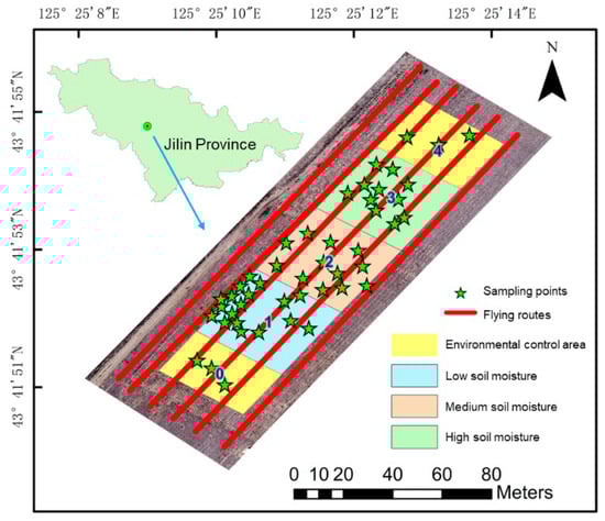
Figure 1.
Overview map of the research area.
The parameters measured in the experiment include microwave radiation brightness temperature data, multispectral data, ridge structure or geometry parameter data, surface roughness data, and on-site ground sampling. These parameters were measured when using the SMAP SCA algorithm to invert the soil moisture [28,29].
The passive drone microwave observation system was employed to obtain the microwave radiation brightness temperature data for the area. The flying routes are represented by the red lines in Figure 1. The setting of the route parameters is based on the instantaneous field of view (IFOV) of the microwave radiometer [36]. The route spacing should be as close to or less than the axis length perpendicular to the observation direction of the radiometer field of view. If an overlap exists between the flight routes, the obtained data will have research value for resolution enhancement.
In this case, work efficiency was considered; therefore, the spacing was set close to the short axis of the IFOV. The flight altitude of the observation system was set to 15 m, considering better special resolution and flight safety. The observation angle was 40°, and the half-beam angle of the antenna was 7.5°. We substituted the flight parameters into the equation as follows:
where
The IFOV of the radiometer in the xoy plane or the ground was obtained as an ellipse with a major axis of 6.8 m and a minor axis of 5.2 m. Thus, the flight path spacing was set to 8 m.
The multi-spectral lens of the drones was employed to obtain the multi-spectral data of the area. The ridge structure parameters, which describe the geometric parameters of the ridge structure, including the ridge height, ridge spacing, and ridge width, were measured using tape measures and rulers in the field. The surface roughness of the soil was measured with a roughness board. Soil samples were collected at the observation points, as marked by the green stars in Figure 1. All raw data were organized to form scientific data and applied for subsequent inversion research.
2.2. Drone-Borne Passive Microwave Observation System
The drone-borne passive microwave observation system adopted in this study was mainly composed of an X-band drone-borne microwave radiometer, a flight platform, and a ground command station, as shown in Figure 2. The X-band has a certain penetration ability for the soil (<5 cm) and is sensitive to changes in surface soil moisture, which can be selected for surface soil moisture inversion in the absence of vegetation cover.
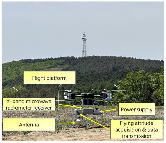
Figure 2.
The drone-borne microwave radiometer and the unmanned aerial vehicle platform.
The radiometer was designed as a total power radiometer, and it adopted the digital automatic gain compensation scheme. This ensured the sensitivity and stability of the receiver, eliminated the complex hardware circuit feedback control link, and reduced the power consumption [36]. Further, it could achieve continuous high-speed acquisition with an integration time of 1 millisecond. Correspondingly, the radiometer could detect radio frequency interference and achieve dual polling fast storage [37], meeting the demand for storing large amounts of data in a very short period without interrupting acquisition. The parameters of the receiver are shown in Table 1.

Table 1.
Parameters of the microwave radiometer receiver.
The raw data measured by the microwave radiometer were the digital values of the output voltage after analog-to-digital conversion, and it could be calibrated into brightness temperature by the two-point calibration method due to the good linearity of the microwave radiometer receiver [41,42]. The two-point calibration method was used to measure liquid nitrogen and blackbody, obtain two sets of output voltage, and establish the relationship with brightness temperature.
The main functions of the ground command station were to control flight and monitor the parameters in real-time. A long-distance wireless transmission link was established through a base station relay, as shown in Figure 3. A cloud server was built and software was developed to monitor the flight and measurement parameters in real time.

Figure 3.
Data flow topology.
A data processing method (Figure 4) considering topography and angle correction was applied in this study [36] which processed the raw data obtained by the drone-borne passive microwave observation system into raster data for subsequent inversion use. The data processing method mainly included seven processes: (1) data extraction, (2) data selection, (3) radiometric calibration, (4) radio frequency interference detection and suppression, (5) GPS interpolation, (6) space projection, and (7) gridding and generating a preview map of the brightness temperature spatial distribution. Note that the TBs in Figure 4 refer to the brightness temperature, and the terms txt, xlsx, and tiff are the data formats at each stage.
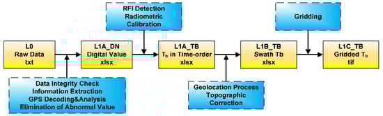
Figure 4.
Diagram of the radiometer data processing.
2.3. Drone-Borne Multispectral Observation and Ground Observation Parameters
The multispectral data of the observation area were obtained through the DJI Mavic-3M multispectral version drone [43]. The M3M aerial survey drone integrates RGB and multispectral cameras, enabling the precise detection of farmland surface parameters and crop growth status. Its multispectral camera has green (560 ± 16 nm), red (650 ± 16 nm), red edge (730 ± 16 nm), and near-infrared (860 ± 26 nm) spectral bands. After the flight, the data were concatenated using the DJI Terra (Agricultural Edition V3.1.4) software to form a multispectral image of the entire observation area, which could be employed for subsequent processing. Thereafter, the image would be resampled to a resolution of 1 m, ensuring compatibility with microwave pixels.
The ground observation in the experiments mainly included surface roughness measurement, soil moisture sampling, and ridge parameter measurement. Pictures of the experiments are shown in Figure 5, including drone-borne radiometer operations, soil sampling, photos of observation targets, and roughness sampling.
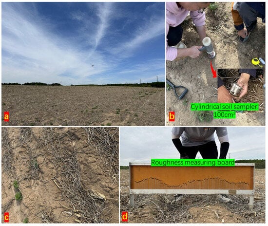
Figure 5.
Pictures of the experiments: (a) drone-borne radiometer; (b) soil sampling; (c) observation target; and (d) roughness measurement.
The surface roughness was crucial for microwave remote sensing inversion of water content [13,44]. When conducting soil moisture inversion, the influence of roughness on surface emissivity was often considered. Notably, high roughness could change surface emissivity, one of the main parameters in passive microwave remote sensing, thereby affecting the signal strength received by the remote sensing sensors. The roughness was measured using a roughness board (Figure 6), which revealed the small undulations on the surface. The board contained 111 needles, with spacing of 1 cm. Five measurement points were selected uniformly for the roughness measurement in each experimental area. The average measurement results would represent the roughness of the area. Three consecutive sets of roughness board photographs were taken at each measurement point. Thereafter, geometric deformation correction was performed, and points were extracted through binarization for calculation.
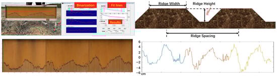
Figure 6.
Measurement and calculation of the soil surface roughness and schematic diagram of ridge structure.
Surface roughness was represented by root mean square height (RMSH) and surface correlation length (CLL) [45,46], which can be expressed as
where is the measured surface height, is the mean value of the heights for the RMSH, CLL is the spacing or interval value when the value of the autocorrelation function is the reciprocal of Euler’s number e, and is number of points measured.
The soil samples were collected on-site (as shown in Figure 5b) and dried using an oven to obtain the true values of the soil-moisture level. We employed a cylindrical soil sampler (volume: 100 cm3) to collect soil from the surface layer (depth: 0–3 cm), placed it in a sealed bag, brought it back to the laboratory for weighing, and heated it to 105 °C in an oven [47,48]. After drying for 24 h, it was taken out to weigh the dry soil mass. The mass water content (MWC) and volumetric water content (VWC) of the soil were calculated by
where and are the masses of the wet and dry soils, respectively, and represents the volume of the cylindrical soil sampler.
Noted that both VWC and MWC were used by the researchers to describe the moisture characteristics of soil, and we found that they showed good consistency. We considered the issue of sampling efficiency in subsequent experiments, also avoiding or reducing some errors caused by long sampling duration. Thus, MWC was chosen as the descriptive parameter.
The ridge structure parameters were measured using tape measures and rulers in the field, as shown in the schematic diagram of Figure 6, including the ridge height, ridge spacing, and ridge width. The ridge height refers to the vertical height from the bottom of the furrow to the top of the ridge, reflecting the degree of protrusion of the ridge body, usually measured with a ruler for 3 repeats; the ridge width typically refers to the horizontal width of the ridge top, that is, the width of the crop planting surface, usually measured with a tape measures for 3 repeats; and the ridge spacing refers to the distance between the centerlines of two adjacent ridges, usually measured by taking the average of the distances between the centerlines of 5 consecutive adjacent ridges using a tape measure.
2.4. Machine Learning Models
The raw data was obtained through the experiments and instruments mentioned above and used as the original input features for the machine learning models after data processing. In this study, the Regression Learner toolbox in MATLAB R2018b was used to train the model.
Extensive research on several machine learning algorithms and their applications has been conducted. However, selecting the right algorithm for certain applications has proven challenging [49]. Thus, in this study, commonly employed machine learning models, including linear, regression tree, support vector regression (SVM), Gaussian process regression (GPR), boosted tree, and random forest (RF), were applied to compare their performances and choose a suitable model. Each model will undergo a certain degree of parameter adjusting, as shown in Figure 7, to achieve the best accuracy.
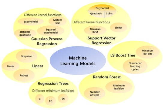
Figure 7.
Machine learning models used and parameters adjusted.
These parameters mainly refer to specific adjustable parameters in each machine learning model. For example, the three different methods in linear models, linear, robust, and stepwise, have different expressions for different data characteristics, mainly reflected in outlier handling strategies, goals and core ideas, variable selection, and other aspects. Regression trees are mainly used for setting different minimum leaf sizes in parameter adjustment. GPR is reflected in the selection of kernel functions and kernel scales, such as exponential kernel, squared exponential kernel, rational quadratic kernel, etc., using optimization strategy of Quasi-Newton. SVM is also reflected in the selection of kernel functions and also different kernel scales, such as linear, Gaussian, and polynomial, using the optimization strategy of Sequential Minimal Optimization. Random forests require adjusting the number of trees and the minimum leaf size. Noted that MATLAB’s TreeBagger was based on Breiman’s random forest algorithm and it did not support automatic hyperparameter tuning (such as grid search), which required manual experimentation with different parameter combinations. The cross-validation folds were set at 10.
2.5. Model Performance Evaluation
The metrics employed to evaluate the model include the root mean square error (RMSE), mean absolute error (MAE), and coefficient of determination (R2). These metrics reflect the predictive ability of the models by calculating the difference between the true and predicted values.
RMSE is the square root of the average sum of the squared errors, which is sensitive to outliers and can reflect the distribution of the prediction errors. MAE is the average of the absolute values of the errors. R2 is defined as the ratio of the variation of the independent variables that have been explained by all the independent variables in the pattern to the total variation of the independent variables. It reflects the reliability of the regression model in explaining the changes in the dependent variable. These metrics can be calculated as follows:
where is the number of samples and , , and are the true value, predicted value, and mean value, respectively.
When selecting parameters or features for the model, an ablation study was adopted to understand and evaluate the contribution of each component or feature of the model to its overall performance. The main goal was to establish a method for controlling the variables. Through the method, we were able to gain a deeper understanding of the models, optimize the model design, and validate the effectiveness of specific features or components.
3. Results
3.1. Experimental Parameter Measurement Results
The experimental area was a rectangle with a dimension of 170 m × 60 m, which included four different soil moisture levels, and the experimental results are shown in Figure 8. Figure 8a,b show the optical and multi-spectrum images of the experimental site, respectively. Using the data processing method mentioned above, the brightness temperature swath data and the gridded data (resampling spatial resolution of 0.00001°) in the test area were obtained, as shown in Figure 8c,d.
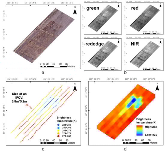
Figure 8.
Display of the flight test results. (a) Optical image; (b) multispectral image; (c) brightness temperature swath data; and (d) brightness temperature gridded data.
Each color point in Figure 8c represents an observation from a microwave radiometer. The IFOV observed each time is approximately an ellipse with major and minor axes of 6.8 m and 5.2 m, respectively. This point represents the position of the projection point of the antenna’s IFOV beam center, and its brightness temperature is represented by color.
Figure 8d reveals that there is a significant difference in the brightness temperature with soil moisture variation. The area with the highest moisture level has the lowest brightness temperature, ranging from 225 K to 250 K. As the moisture level decreases, the brightness gradually increases. The brightness temperatures in the medium and the lowest moisture level areas range from 260 K to 270 K and 270 K to 280 K, respectively; the difference is quite small. As the control group, the environment had the lowest soil moisture level, attributed to a lack of watering, with a brightness temperature of ~280 K.
The measurement results of the ridge structure parameters and the surface roughness are shown in Figure 9. The ridge spacing, ridge height, and ridge width are distributed between 65 and 80 cm, 4 and 10 cm, and 45 and 55 cm, respectively; The RMSH and CLL are distributed at 0.5–2 cm and 4–10 cm, respectively.
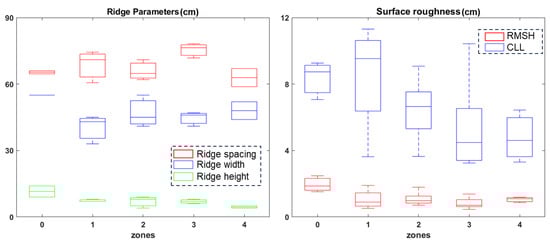
Figure 9.
Measurement results of the ridge structure parameters and surface roughness.
The soil samples were collected on-site and dried using an oven to obtain the true value for the soil moisture level. The calculated VWC and MWC exhibited good consistency (with an R2 of 0.86); thus, MWC was selected for the model validation in this study, as shown in Figure 10. The green dots represent the original sampled values, whereas the red dots represent the mean. The mean surface MWCs of the three experimental groups were 11.1%, 13.9%, and 19.3%, respectively, whereas the surface MWCs of the two environmental control groups were 8.3% and 9.2%. The MWC distribution is displayed in ascending order in the lower right corner of the graph.
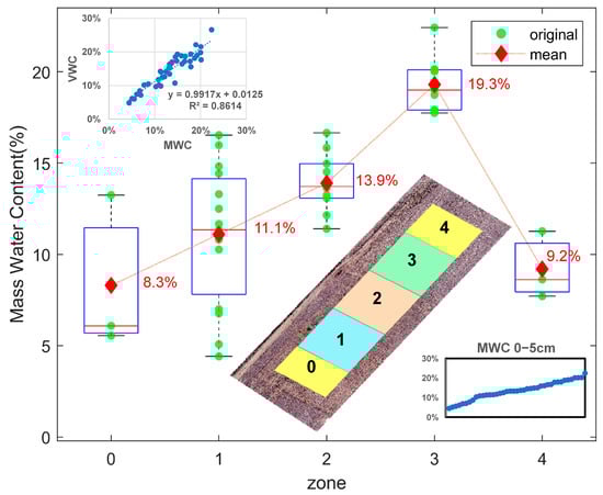
Figure 10.
Soil moisture distribution in in situ sampling.
3.2. Machine Learning and Soil Moisture Inversion Results
Machine learning models have developed rapidly in recent years. In this study, we first implemented the most commonly used models. Next, we comprehensively compared their performances and selected the model with the best performance. Finally, we employed this model for ablation experiments, selecting sensitive parameters.
Each method was regressed 100 times, after which the mean values of the RMSE, MAE, and R2 were calculated to eliminate randomness. For each experiment, 80% of the selected data was adopted as the training set and 20% as the validation set without replacement. The input consists of 10 features, namely ridge spacing, ridge height, ridge width, RMSH, CLL, four spectrum bands (red, green, red edge, and NIR), and brightness temperature.
The regression results and the statistical results of the training and validation sets obtained through the regression of different models are shown in Figure 11 and Table 2, respectively. The table shows that the performance of the models was relatively good, with the soil moisture RMSE reaching the recognized 4% level and MAE remaining at a very low level.
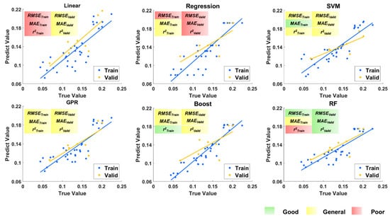
Figure 11.
Training–validation dataset: RMSE, MAE, and R2 values for 100 replications of different models.
Table 2.
Training–validation datasets: RMSE, MAE, and R2 values for 100 replications of different models.
For the best performance both in training and validation, the random forest was selected as the regression algorithm. Out of Bag (OOB) error, a method for evaluating the performance of random forest models, was adopted. The results were similar to those for cross-validation. The OOB error calculation was obtained synchronously during the training process [50]. The OOB error results of the experiment are shown in Figure 12. The horizontal axis represents the number of decision trees, and the vertical axis represents the OOB error. The results indicate that when the number of trees grew to around 30, the OOB error could already be maintained at a stable and low level.

Figure 12.
Out-of-bag error rate of random forest.
We completed the model selection process and proceeded with model-based feature selection. In decision tree-based ensemble algorithms, correlation analysis and feature importance are commonly used as an evaluation metric. Correlation analysis focuses on the relationships between features, while feature importance focuses on the relationship between features and the target. The results of Pearson correlations between features are shown in Figure 13. The feature importance results obtained using the random forest algorithm are shown in Figure 14.
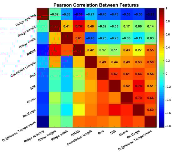
Figure 13.
Pearson correlation between features.
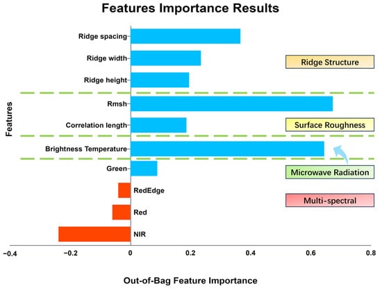
Figure 14.
Out of bag feature importance.
The statistical results for the regression models fitted with the training and validation sets obtained using different input features are shown in Table 3. The statistical results are represented by different colors to indicate their advantages and disadvantages, with green, yellow, and red representing the best, medium, and worst.
Table 3.
Training–validation datasets: RMSE, MAE, and R2 values for 100 replications of different inputs features.
Since the parameters for models fitted with the training and validation sets are consistent, we only presented the results of the models fitted with the training set in the image for simplicity. The RMSE and MAE are presented in the form of bar charts (main axis on the left) and the R2 in the form of line charts (sub axis on the right), as shown in Figure 15. The smaller the RMSE and MAE values, the smaller the deviation. The larger the R2 score, the better the regression effect. Thus, two different forms of charts were employed to avoid confusion.

Figure 15.
Training results: RMSE, MAE, and R2 values for 100 replications of different features.
The microwave radiation brightness temperature of all pixels was extracted and used as inputs of the trained model to invert the soil moisture in the experimental area, as shown in Figure 16. The figure on the left shows the spatial distribution of the soil moisture inversion, ranging from 8% to 20%.

Figure 16.
Soil moisture inversion results.
The upper right figure shows the relationship between the input brightness temperature and the MWC value. The blue dots represent the predicted values of all pixels, and the green hexagrams represent the measured true values. Evidently, the brightness temperature of the soil decreases significantly as the MWC increases.
4. Discussion
4.1. Experimental Parameter Measurement
From the parameters of the ridge structure that describe the geometric form, most zones maintained good consistency as all the values were within the confidence intervals of the 3σ (the mean value ± three times the standard deviation). In terms of surface roughness, the RMSH of Zone 0 was significantly higher than those of the other zones. However, the CLL does not show a clear trend. For most parameters, good consistency was maintained with slight differences. Therefore, it can be concluded that the impact of these parameters as inputs on the accuracy of the soil moisture inversion model was negligible.
The results showed that the MWC gradient produced by watering was ideal, with a distance among the gradients that met the experimental requirements. These raw values would be employed as the validation true values. Moreover, some heterogeneities were observed within the same region, which made it difficult to achieve complete uniformity in relatively “large-scale” control experiments. This is an issue that needs to be resolved in future experiments.
4.2. Machine Learning and Soil Moisture Inversion
From the statistical results of 100 replications of different models shown in Figure 11 and Table 2, random forest exhibited the most stable and excellent performance on the validation set, particularly outperforming other models significantly in terms of the R2 metric (0.65), while also demonstrating good performance in terms of RMSE and MAE. support vector regression demonstrated excellent overall performance, maintaining a high level on both the training set and the validation set, particularly excelling in terms of the MAE metric. The boosted tree exhibited excellent R2 performance on the training set (0.8506), but its performance significantly decreases on the validation set (0.4296), indicating a potential overfitting issue. Linear regression and regression trees performed relatively poorly on the validation set, which may indicate that they are not suitable for the current task. Gaussian process regression performs moderately, but its stability is inferior to that of SVR and random forest. Furthermore, based on the standard deviation and confidence interval calculated from 100 random splits, it could be observed that the distribution was relatively concentrated, indicating that the model performance was stable across repeated validations.
From the results of OOB error tests, the OOB error decreases as the number of trees increases within a certain range, but it was also necessary to consider the balance between computational efficiency and error. The number of trees finally used was 100 and the minimum leaf size was 5 which had the lowest OOB error. The random forest model itself has the ability to resist overfitting, but having too many trees may lead to wastage of computational resources.
The results of Pearson correlations between features are shown in Figure 13. There was a generally moderate to strong positive correlation among spectral features, indicating that these bands might have overlapping information in their measurements. The correlation patterns between ridge features (spacing, height, and width) and spectral features were inconsistent, with some showing positive correlations and others showing negative correlations. Features with weak correlations with brightness temperature (such as ridge width) might have limited contributions in predicting brightness temperature.
Feature importance is used to evaluate the importance of each input feature (predictor variable) in the random forest model, and the variable importance score is calculated through permutation testing, which can assist in feature selection. The results indicate that the passive microwave radiation brightness temperature and surface roughness contributed significantly to the accuracy of the training model, which is consistent with prior knowledge [51,52]. The parameters of the ridge structure also had a certain impact on the regression results of the soil moisture, and the impact of different multispectral bands on the regression results was relatively small, even negative.
Evidently, prior knowledge and experimental results demonstrate the importance of soil surface roughness in soil moisture inversion. Its importance is mainly manifested in its influence on the surface equivalent dielectric constant, the radar backscattering coefficient, and, more significantly, the shorter wavelength band. However, currently, the main method for accurately obtaining surface roughness is on-site ground measurement, which is inefficient and cannot be widely promoted. Although we attempted to employ drone-borne LiDAR to obtain point cloud data for modeling, the instability during the unmanned aerial vehicle flight resulted in a few centimeters of error, which greatly affected the measurement results. There is no other good technical method yet for efficiently obtaining microwave-scale surface area data. Further, the surface roughness was no longer included in subsequent experiments and discussions in this study.
The feature importance results could assist in feature selection; however, the physical meaning of these features should be considered, and some parameters may appear in groups. Therefore, when conducting ablation experiments, the design should be based on the characteristics being explored.
From Figure 15, the results indicate the following: (1) When all features were used as input parameters, RMSE and MAE were the smallest and R2 was the largest. Thus, the regression results were the best. (2) When any of the parameters were removed, the RMSE and MAE increased, R2 decreased, and the regression results deteriorated. In particular, the effect of removing the microwave radiation brightness temperature alone was the worst, which verified the importance of the microwave characteristic parameters for the model. (3) When only one single parameter was employed as the feature input, the regression results deteriorated. When only the microwave brightness temperature was employed as an input, the best performance was obtained, similar to or slightly better than the results obtained when two parameter inputs were adopted, which indicated that the brightness temperature had more importance than the multispectral data.
The regression effect obtained when the microwave radiation brightness temperature is adopted as a single parameter was good, although the accuracy could be further improved by adding other auxiliary parameters. Further, the practical significance of these features, difficulty of parameter acquisition, cost of application experiments, and universality of the entire model were considered. There was a tradeoff between the experimental cost and the workload of parameter acquisition and inversion accuracy.
In addition, we strongly agreed with the importance of surface emissivity in soil moisture inversion, but other auxiliary parameters such as soil texture were difficult to obtain. The effective temperature of soil, or the physical temperature of soil, is also a difficult parameter to obtain at high-resolution regional scales. A relatively fast way now was to use unmanned aerial vehicle thermal infrared cameras to obtain surface temperature, but, similarly, there was also a difference in the emissivity of the infrared band due to the influence of soil moisture and there might also be some uncertainty in the digital value of non-constant temperature lens output after calibration. The emissivity calculated using this temperature is actually the ratio of emissivity in the microwave to the thermal infrared bands, which can be expressed as
Both and Tb have shown consistent trends with MWC. Thus, we decided to use the microwave radiation brightness temperature as the only input.
The soil moisture in Zone 3, designed as a high-moisture area, was significantly higher than those in other zones. Conversely, the soil moisture in the environmental area, the control group, was the lowest. Zones 1 and 2 were designed as low- and medium-moisture areas, and their soil moisture contents were determined. Interestingly, there was one strip (marked in red rectangle) in Zone 2 with significantly higher moisture content than the other regions. This might be caused by the excessive watering in Zone 3, which led to saturation. Additionally, there is a slope causing water to flow along the ridge to Zone 2.
As shown in the result of soil moisture inversion, the range of the brightness temperature extreme values corresponding to the sampled true values used for the training set was smaller than the input range used for prediction, which might result in some uncertainty in the predictions outside the range, mainly reflected in the high brightness temperature region. The absolute error between the measured true value and the predicted value at the sampling point is shown in the lower right figure. We divided it into four intervals: <10%, 10–15%, 15–20%, and >20%. We calculated the MAE values, which were 3.58%, 1.12%, 1.67%, and 1.30%, respectively. The results showed that in the low soil moisture-level area, the inversion error was relatively large, whereas in the medium–high soil moisture-level area, the inversion effect was improved.
5. Conclusions
In this study, a control experimental field with different soil moisture gradients was established. A drone-borne passive microwave observation system of the X-band was developed and employed to obtain the regional brightness temperature. Machine learning models and input features were studied and applied for the soil moisture inversion. The results indicated that by using the microwave radiation brightness temperature as the input parameter, the models could achieve good regression accuracy and effectively complete the inversion tasks. The RMSE and R2 scores of the model fitted with the training set reached 2.47% and 0.74%, respectively. Finally, the soil moisture distribution in the experimental area was obtained.
By designing control experiments, we successfully verified the feasibility of the drone-borne passive microwave remote sensing observation system in high-resolution soil moisture inversion applications and achieved good results. The accuracy of the soil-moisture inversion was higher than 4%, generating high-resolution soil moisture distribution in the region, which could meet the monitoring needs of precision agriculture plots. The model did not rely on ground parameter measurements and exhibited generalization ability.
There are still some shortcomings in this study, which is an issue that we will further focus on. One is the model’s generalization ability. The generalizability of training models is influenced by various factors, including different soil textures and soil structures. In future work, more experiments will be conducted to enhance the model’s generalization ability. Another limitation is the scale matching problem, which refers to the consistency between the optimal observation scale and the spatiotemporal scale of geographic phenomena at high resolutions. Finally, the points-to-surface scale transformation problem observed during data processing should also be considered.
Drone-borne passive microwave remote sensing observation could be a new technical approach for high-spatial resolution monitoring, filling the scale gap between airborne and ground-based observations. The proposed model could achieve near-surface observation of parameters, providing stable, reliable, and high-resolution data support for the establishment, improvement, and validation of models. Correspondingly, the model could be applied for precise agricultural parameter inversion at the field scale. The developed algorithms could be applied to satellites and employed for the ground verification of satellites. We can say with certainty that if more training data is obtained in the future, more frameworks or models can be developed with enhanced generalization ability.
Author Contributions
Conceptualization, methodology, software, validation, formal analysis, investigation, data curation, and writing—original draft preparation: T.J. and X.W.; visualization: L.L.; writing—review and editing: X.Z.; supervision, resources, project administration, and funding acquisition: X.L. All authors have read and agreed to the published version of the manuscript.
Funding
This research was funded by the Strategic Priority Research Program of the Chinese Academy of Sciences (grant number XDA28110502), the Jilin Province Innovation and Entrepreneurship Talent Project (No. 2023QN15), the Common Application Support Platform for National Civil Space Infrastructure Land Observation Satellites (Grant No. “2017-000052-73-01-001735”), and the Science and Technology Development Plan Project of Jilin Province (No. YDZJ202501ZYTS565).
Data Availability Statement
No new data were created or analyzed in this study. Data sharing is not applicable to this article.
Acknowledgments
Besides the authors of the paper, we would also like to thank those who have contributed to field observations and data processing, including but not limited to Yanling Wei, Zhuangzhuang Feng, Xinrui Li, Hailong Li, Han Yang, Chunzhe Yu, Xiaopeng Zhang, Peng Gao, Yisheng Wang, and Yijing Li.
Conflicts of Interest
The authors declare no conflicts of interest.
Abbreviations
| SSM | Surface soil moisture |
| SCA | Single-channel algorithm |
| IFOV | Instantaneous field of view |
| RMSH | Root mean square height |
| CLL | Correlation length |
| MWC | Mass water content |
| VWC | Volumetric water content |
| SVM | Support vector regression |
| GPR | Gaussian process regression |
| RF | Random forest |
| RMSE | Root mean square error |
| MAE | Mean absolute error |
| OOB | Out of bag |
References
- Bras, R.L. Complexity and Organization in Hydrology: A Personal View. Water Resour. Res. 2015, 51, 6532–6548. [Google Scholar] [CrossRef]
- Chawla, I.; Karthikeyan, L.; Mishra, A.K. A Review of Remote Sensing Applications for Water Security: Quantity, Quality, and Extremes. J. Hydrol. 2020, 585, 124826. [Google Scholar] [CrossRef]
- Li, L.; Li, X.; Zheng, X.; Li, X.; Jiang, T.; Ju, H.; Wan, X. The Effects of Declining Soil Moisture Levels on Suitable Maize Cultivation Areas in Northeast China. J. Hydrol. 2022, 608, 127636. [Google Scholar] [CrossRef]
- Guo, T.; Zheng, J.; Wang, C.; Tao, Z.; Zheng, X.; Wang, Q.; Li, L.; Feng, Z.; Wang, X.; Li, X.; et al. A Cloud Framework for High Spatial Resolution Soil Moisture Mapping from Radar and Optical Satellite Imageries. Chin. Geogr. Sci. 2023, 33, 649–663. [Google Scholar] [CrossRef]
- Liu, Q.; Guo, H.; Zhang, J.; Li, S.; Li, J.; Yao, F.; Mahecha, M.D.; Peng, J. Global Assessment of Terrestrial Productivity in Response to Water Stress. Sci. Bull. 2024, 69, 2352–2356. [Google Scholar] [CrossRef]
- Holzman, M.E.; Rivas, R.; Piccolo, M.C. Estimating Soil Moisture and the Relationship with Crop Yield Using Surface Temperature and Vegetation Index. Int. J. Appl. Earth Obs. Geoinf. 2014, 28, 181–192. [Google Scholar] [CrossRef]
- Wu, X.; Ma, W.; Xia, J.; Bai, W.; Jin, S.; Calabia, A. Spaceborne GNSS-R Soil Moisture Retrieval: Status, Development Opportunities, and Challenges. Remote Sens. 2020, 13, 45. [Google Scholar] [CrossRef]
- Zakharov, I.; Kohlsmith, S.; Hornung, J.; Charbonneau, F.; Bobby, P.; Howell, M. Surface Soil Moisture Estimation from Time Series of RADARSAT Constellation Mission Compact Polarimetric Data for the Identification of Water-Saturated Areas. Remote Sens. 2024, 16, 2664. [Google Scholar] [CrossRef]
- Bhogapurapu, N.; Dey, S.; Homayouni, S.; Bhattacharya, A.; Rao, Y.S. Field-Scale Soil Moisture Estimation Using Sentinel-1 GRD SAR Data. Adv. Space Res. 2022, 70, 3845–3858. [Google Scholar] [CrossRef]
- Engman, E.T.; Chauhan, N. Status of Microwave Soil Moisture Measurements with Remote Sensing. Remote Sens. Environ. 1995, 51, 189–198. [Google Scholar] [CrossRef]
- Thaggahalli Nagaraju, S.K.; Pathak, A.A. Retrieving Surface and Rootzone Soil Moisture Using Microwave Remote Sensing. J. Indian Soc. Remote Sens. 2024, 52, 1415–1430. [Google Scholar] [CrossRef]
- Wang, Y.; Zhao, J.; Guo, Z.; Yang, H.; Li, N. Soil Moisture Inversion Based on Data Augmentation Method Using Multi-Source Remote Sensing Data. Remote Sens. 2023, 15, 1899. [Google Scholar] [CrossRef]
- Zheng, X.; Zhao, K. A Method for Surface Roughness Parameter Estimation in Passive Microwave Remote Sensing. Chin. Geogr. Sci. 2010, 20, 345–352. [Google Scholar] [CrossRef]
- Derksen, C.; Walker, A.; LeDrew, E.; Goodison, B. Combining SMMR and SSM/I Data for Time Series Analysis of Central North American Snow Water Equivalent. J. Hydrometeorol. 2003, 4, 304–316. [Google Scholar] [CrossRef]
- Kawanishi, T.; Sezai, T.; Ito, Y.; Imaoka, K.; Takeshima, T.; Ishido, Y.; Shibata, A.; Miura, M.; Inahata, H.; Spencer, R.W. The Advanced Microwave Scanning Radiometer for the Earth Observing System (AMSR-E), NASDA’s Contribution to the EOS for Global Energy and Water Cycle Studies. IEEE Trans. Geosci. Remote Sens. 2003, 41, 184–194. [Google Scholar] [CrossRef]
- Li, S.; Xing, M.; Dong, T. An Apparent Thermal Inertia Based Trapezoid Model for Downscaling of ESA CCI Soil Moisture Products. IEEE J. Sel. Top. Appl. Earth Obs. Remote Sens. 2025, 18, 4473–4486. [Google Scholar] [CrossRef]
- Zheng, X.; Feng, Z.; Xu, H.; Sun, Y.; Li, L.; Li, B.; Jiang, T.; Li, X.; Li, X. A New Soil Moisture Retrieval Algorithm from the L-Band Passive Microwave Brightness Temperature Based on the Change Detection Principle. Remote Sens. 2020, 12, 1303. [Google Scholar] [CrossRef]
- Wang, W.; Ma, C.; Wang, X.; Feng, J.; Dong, L.; Kang, J.; Jin, R.; Li, X. A Soil Moisture Experiment for Validating High-Resolution Satellite Products and Monitoring Irrigation at Agricultural Field Scale. Agric. Water Manag. 2024, 304, 109071. [Google Scholar] [CrossRef]
- Archer, F.; Shutko, A.M.; Coleman, T.L.; Haldin, A.; Novichikhin, E.P.; Sidorov, I.A. Introduction, Overview, and Status of the Microwave Autonomous Copter System (MACS). In Proceedings of the International Geoscience and Remote Sensing Symposium, Athens, Greece, 20–24 September 2004. [Google Scholar] [CrossRef]
- Brown, S.T.; Lambrigtsen, B.; Denning, R.F.; Gaier, T.; Kangaslahti, P.; Lim, B.H.; Tanabe, J.M.; Tanner, A.B. The High-Altitude MMIC Sounding Radiometer for the Global Hawk Unmanned Aerial Vehicle: Instrument Description and Performance. IEEE Trans. Geosci. Remote Sens. 2011, 49, 3291–3301. [Google Scholar] [CrossRef]
- Acevo-Herrera, R.; Aguasca, A.; Bosch-Lluis, X.; Camps, A.; Martínez-Fernández, J.; Sánchez-Martín, N.; Pérez-Gutiérrez, C. Design and First Results of an UAV-Borne L-Band Radiometer for Multiple Monitoring Purposes. Remote Sens. 2010, 2, 1662–1679. [Google Scholar] [CrossRef]
- Houtz, D.; Naderpour, R.; Schwank, M. Portable L-Band Radiometer (PoLRa): Design and Characterization. Remote Sens. 2020, 12, 2780. [Google Scholar] [CrossRef]
- Zhang, R.; Nayak, A.; Houtz, D.; Watts, A.; Soltanaghai, E.; Alipour, M. Evaluation of Soil Moisture Retrievals from a Portable L-Band Microwave Radiometer. Remote Sens. 2024, 16, 4596. [Google Scholar] [CrossRef]
- Horton, D.; Johnson, J.T.; Al-Khaldi, M.; Park, J.; Bindlish, R. A Study of the Second Order Small Slope Approximation for L-Band Backscattering from Soil Surfaces. In Proceedings of the IEEE International Geoscience and Remote Sensing Symposium, Athens, Greece, 5 September 2024; pp. 4354–4357. [Google Scholar] [CrossRef]
- Oh, Y. Quantitative Retrieval of Soil Moisture Content and Surface Roughness from Multipolarized Radar Observations of Bare Soil Surfaces. IEEE Trans. Geosci. Remote Sens. 2004, 42, 596–601. [Google Scholar] [CrossRef]
- Song, K. Multilayer Soil Model for Improvement of Soil Moisture Estimation Using the Small Perturbation Method. J. Appl. Remote Sens. 2009, 3, 033567. [Google Scholar] [CrossRef]
- Cui, K.; Xing, M.; Shang, J.; Zhou, X.; Wang, J. Enhanced L-MEB Model for Soil Moisture Retrieval over Soybean Fields during the Growing Season. IEEE Trans. Geosci. Remote Sens. 2025, 63, 4409216. [Google Scholar] [CrossRef]
- Dong, J.; Crow, W.T.; Bindlish, R. The Error Structure of the SMAP Single and Dual Channel Soil Moisture Retrievals. Geophys. Res. Lett. 2018, 45, 758–765. [Google Scholar] [CrossRef]
- Chan, S.K.; Bindlish, R.; O’Neill, P.E.; Njoku, E.; Jackson, T.; Colliander, A.; Chen, F.; Burgin, M.; Dunbar, S.; Piepmeier, J.; et al. Assessment of the SMAP Passive Soil Moisture Product. IEEE Trans. Geosci. Remote Sens. 2016, 54, 4994–5007. [Google Scholar] [CrossRef]
- Ali, I.; Greifeneder, F.; Stamenkovic, J.; Neumann, M.; Notarnicola, C. Review of Machine Learning Approaches for Biomass and Soil Moisture Retrievals from Remote Sensing Data. Remote Sens. 2015, 7, 16398–16421. [Google Scholar] [CrossRef]
- Sungmin, O.; Orth, R. Global Soil Moisture Data Derived through Machine Learning Trained with In-Situ Measurements. Sci. Data 2021, 8, 170. [Google Scholar] [CrossRef] [PubMed]
- Teshome, F.T.; Bayabil, H.K.; Schaffer, B.; Ampatzidis, Y.; Hoogenboom, G. Improving Soil Moisture Prediction with Deep Learning and Machine Learning Models. Comput. Electron. Agric. 2024, 226, 109414. [Google Scholar] [CrossRef]
- Greifeneder, F.; Notarnicola, C.; Wagner, W. A Machine Learning-Based Approach for Surface Soil Moisture Estimations with Google Earth Engine. Remote Sens. 2021, 13, 2099. [Google Scholar] [CrossRef]
- Ma, H.; Zeng, J.; Zhang, X.; Peng, J.; Li, X.; Fu, P.; Cosh, M.H.; Letu, H.; Wang, S.; Chen, N.; et al. Surface Soil Moisture from Combined Active and Passive Microwave Observations: Integrating ASCAT and SMAP Observations Based on Machine Learning Approaches. Remote Sens. Environ. 2024, 308, 114197. [Google Scholar] [CrossRef]
- Wang, L.; Gao, Y. Soil Moisture Retrieval from Sentinel-1 and Sentinel-2 Data Using Ensemble Learning over Vegetated Fields. IEEE J. Sel. Top. Appl. Earth Obs. Remote Sens. 2023, 16, 1802–1814. [Google Scholar] [CrossRef]
- Wan, X.; Li, X.; Jiang, T.; Zheng, X.; Li, L.; Wang, X. High-Resolution Imaging of Radiation Brightness Temperature Obtained by Drone-Borne Microwave Radiometer. Remote Sens. 2023, 15, 832. [Google Scholar] [CrossRef]
- Wan, X.; Li, X.; Jiang, T.; Zheng, X.; Li, X.; Li, L. A Fast Storage Method for Drone-Borne Passive Microwave Radiation Measurement. Sensors 2021, 21, 6767. [Google Scholar] [CrossRef]
- Lei, F.; Volkan, S.; Mehmet, K.; Ali, C.G.; Moorhead, R.J.; Boyd, D. Machine-Learning Based Retrieval of Soil Moisture at High Spatio-Temporal Scales Using CYGNSS and SMAP Observations. In Proceedings of the Geoscience and Remote Sensing Symposium, Waikoloa, HI, USA, 26 September–2 October 2020. [Google Scholar] [CrossRef]
- Li, Z.; Yuan, Q.; Zhang, L. Geo-Intelligent Retrieval Framework Based on Machine Learning in the Cloud Environment: A Case Study of Soil Moisture Retrieval. IEEE Trans. Geosci. Remote Sens. 2023, 61, 1–15. [Google Scholar] [CrossRef]
- Xue, Z.; Zhang, Y.; Zhang, L.; Li, H. Ensemble Learning Embedded with Gaussian Process Regression for Soil Moisture Estimation: A Case Study of the Continental U.S. IEEE Trans. Geosci. Remote Sens. 2022, 60, 4508817. [Google Scholar] [CrossRef]
- Luan, H.; Zhao, K. Error Analysis and Accuracy Validation of Two-Point Calibration for Microwave Radiometer Receiver. J. Infrared Millim. Waves 2007, 26, 289–292. [Google Scholar]
- Xu, W.T.; Yang, C.T. Microwave Radiometer Calibration and Its Error Analysis. In Proceedings of the Conference on Precision Electromagnetic Measurements, Ibaraki, Japan, 6 August 2002; pp. 390–391. [Google Scholar] [CrossRef]
- DJI Mavic 3M Manual, V1.7 ed.; Dajiang Innovation: Shenzhen, China, 2024; Available online: https://dl.djicdn.com/downloads/DJI_Mavic_3_Enterprise/20240606/DJI_Mavic_3M_User_Manual_CHS.pdf (accessed on 1 July 2025).
- Zheng, X.; Feng, Z.; Li, L.; Li, B.; Jiang, T.; Li, X.; Li, X.; Chen, S. Simultaneously Estimating Surface Soil Moisture and Roughness of Bare Soils by Combining Optical and Radar Data. Int. J. Appl. Earth Obs. Geoinf. 2021, 100, 102345. [Google Scholar] [CrossRef]
- Tsang, L.; Kong, J.; Ding, K.-H. Scattering of Electromagnetic Waves: Theories and Applications; Wiley: Hoboken, NJ, USA, 2000. [Google Scholar] [CrossRef]
- Franceschetti, G.; Riccio, D. Scattering, Natural Surfaces, and Fractals; Elsevier: Amsterdam, The Netherlands, 2007. [Google Scholar] [CrossRef]
- Schmugge, T.J.; Jackson, T.J.; McKim, H.L. Survey of Methods for Soil Moisture Determination. Water Resour. Res. 1980, 16, 961–979. [Google Scholar] [CrossRef]
- Stafford, J.V. Remote, Non-Contact and In-Situ Measurement of Soil Moisture Content: A Review. J. Agric. Eng. Res. 1988, 41, 151–172. [Google Scholar] [CrossRef]
- Olson, R.S.; Cava, W.L.; Mustahsan, Z.; Varik, A.; Moore, J.H. Data-Driven Advice for Applying Machine Learning to Bioinformatics Problems. Pac. Symp. Biocomput. 2018, 23, 192–203. [Google Scholar] [PubMed]
- Breiman, L. Random Forests. Mach. Learn. 2001, 45, 5–32. [Google Scholar] [CrossRef]
- Piles, M.; Vall-llossera, M.; Camps, A.; Talone, M.; Monerris, A. Analysis of a Least-Squares Soil Moisture Retrieval Algorithm from L-Band Passive Observations. Remote Sens. 2010, 2, 352–374. [Google Scholar] [CrossRef]
- Martinez-Agirre, A.; Alvarez-Mozos, J.; Lievens, H.; Verhoest, N.E.C. Influence of Surface Roughness Measurement Scale on Radar Backscattering in Different Agricultural Soils. IEEE Trans. Geosci. Remote Sens. 2017, 55, 5925–5936. [Google Scholar] [CrossRef]
Disclaimer/Publisher’s Note: The statements, opinions and data contained in all publications are solely those of the individual author(s) and contributor(s) and not of MDPI and/or the editor(s). MDPI and/or the editor(s) disclaim responsibility for any injury to people or property resulting from any ideas, methods, instructions or products referred to in the content. |
© 2025 by the authors. Licensee MDPI, Basel, Switzerland. This article is an open access article distributed under the terms and conditions of the Creative Commons Attribution (CC BY) license (https://creativecommons.org/licenses/by/4.0/).