Article

Sandy Beach Extraction Method Based on Multi-Source Data and Feature Optimization: A Case in Fujian Province, China

1
Key Laboratory of Land Surface Pattern and Simulation, Institute of Geographic Sciences and Natural Resources Research, Chinese Academy of Sciences, Beijing 100101, China
2
University of Chinese Academy of Sciences, Beijing 100049, China
*
Author to whom correspondence should be addressed.
Remote Sens. 2025, 17(16), 2754; https://doi.org/10.3390/rs17162754
Submission received: 3 June 2025 / Revised: 26 July 2025 / Accepted: 5 August 2025 / Published: 8 August 2025
(This article belongs to the Section Ocean Remote Sensing)

Abstract

Sandy beaches are vital geomorphic units with ecological, social, and economic significance, playing a key role in coastal protection and ecosystem regulation. However, they are increasingly threatened by climate change and human activities, highlighting the need for large-scale, high-precision monitoring to support sustainable management. Existing remote-sensing-based sandy beach extraction methods face challenges such as suboptimal feature selection and reliance on single data sources, limiting their generalization and accuracy. This study proposes a novel sandy beach extraction framework that integrates multi-source data, feature optimization, and collaborative modeling, with Fujian Province, China, as the study area. The framework combines Sentinel-1/2 imagery, nighttime light data, and terrain data to construct a comprehensive feature set containing 44 spectrum, index, polarization, texture, and terrain variables. The optimal feature subsets are selected using the Recursive Feature Elimination (RFE) algorithm. Six machine learning models—Random Forest (RF), Extreme Gradient Boosting (XGBoost), Light Gradient Boosting Machine (LGBM), Gradient Boosting Machine (GBM), Adaptive Boosting (AdaBoost), and Categorical Boosting (CatBoost)—along with an ensemble learning model, are employed for comparative analysis and performance optimization. The results indicate the following. (1) All models achieved the best performance when integrating all five types of features, with the average overall F1-score and accuracy reaching 0.9714 and 0.9733, respectively. (2) The number of optimal features selected by RFE varied by model, ranging from 19 to 36. The ten most important features across models were Band 2 (B2), Elevation, Band 3 (B3), VVVH_SUM, Spatial Average (SAVG), VH, Enhanced Water Index (EWI), Slope, Variance (VAR), and Normalized Difference Vegetation Index (NDVI). (3) The ensemble learning model outperformed all others, achieving an average overall accuracy, precision, recall, and F1-score of 0.9750, 0.9733, 0.9725, and 0.9734, respectively, under the optimal feature subset. A total of 555 sandy beaches were extracted in Fujian Province, covering an area of 43.60 km2 with a total perimeter of 1263.59 km. This framework demonstrates strong adaptability and robustness in complex coastal environments, providing a scalable solution for intelligent sandy beach monitoring and refined resource management.

1. Introduction

Sandy beaches, as vital natural geomorphic units, possess ecological, economic, and social value, playing an irreplaceable role in coastal protection, ecosystem regulation, and supporting human activities [1]. They can effectively buffer storm surges and wave energy, regulate regional climate, provide critical habitats for coastal biodiversity, and support key industries such as tourism, fisheries, and real estate development [2]. Coastal sandy beach resources have become a fundamental basis for human settlement, economic development, and ecological balance [3]. However, with the intensification of global climate change and the accelerating pace of coastal urbanization, coastal sandy beaches and their ecosystems are increasingly affected by both natural and anthropogenic disturbances. These impacts lead to significant spatiotemporal dynamics of sandy beaches, degradation of biological habitats, and gradual loss of ecological functions [4]. Therefore, accurate and dynamic monitoring of the spatiotemporal patterns of sandy beaches is of great importance for supporting sustainable development in coastal areas and maintaining the stability of coastal ecosystems.
Remote sensing technology offers advantages such as timeliness, efficiency, and wide-area coverage. The use of optical remote sensing imagery has significantly improved the efficiency of sandy beach extraction, with methods gradually evolving from manual visual interpretation to automated extraction. In recent years, research on automated sandy beach extraction methods has mainly focused on two categories: threshold-based methods and classifier-based methods [5,6]. Threshold-based approaches typically involve analyzing spectrum, texture, or geometric differences between sandy beaches and other land cover types to define fixed or adaptive thresholds for rapid segmentation. These methods are computationally efficient and easy to implement, making them suitable for large-scale preliminary mapping tasks. However, in areas with complex backgrounds or similar spectrum characteristics, threshold-based methods are prone to misclassification or omission, leading to limited accuracy [7]. Classifier-based methods, on the other hand, rely on machine learning or deep learning frameworks, which can integrate spectrum, spatial, and texture features from multi-source data. Algorithms such as Random Forest (RF), Support Vector Machine (SVM), and convolutional neural networks like U-Net are commonly employed to build classification models and have demonstrated clear advantages in improving extraction accuracy. Nevertheless, these methods are heavily dependent on feature engineering, requiring manual extraction and integration of diverse features. Moreover, the performance of such models is highly sensitive to sample quality and may degrade under conditions where feature boundaries are ambiguous or background interference is significant [8]. Therefore, effectively mining and integrating sandy beach features for the accurate and robust extraction of sandy beach contours remains a key challenge in optimizing current beach extraction methods.
Although sandy beaches possess distinct topographic and spectral characteristics, their extraction processes remain susceptible to various disturbances, such as spectrum confusion, object overlap, and terrain undulation. As a result, relying solely on a single type of data or feature makes it difficult to achieve high-precision and robust identification [9]. In recent years, the development of multi-source satellite data—such as optical and radar remote sensing—has enriched the multidimensional characterization of sandy beaches. Integrating diverse features into classifier algorithms has become a key approach for improving the accuracy of automated beach extraction. Studies have shown that combining topographic data with optical imagery can help mitigate spectrum confusion [10], while incorporating Synthetic Aperture Radar (SAR) data—capable of all-weather imaging—can significantly enhance the recognition performance under complex conditions [11]. However, current feature selection mechanisms and model generalization capabilities still struggle to support automated sandy beach extraction across multiple regions and time scales. On the one hand, high-dimensional and redundant features limit the transferability and stability of models in practical applications. On the other hand, under complex and dynamic beach morphologies and remote sensing conditions, existing methods still face challenges in robustness and generalization [12,13]. Recursive Feature Elimination (RFE), an effective feature selection method, optimizes input subsets by iteratively eliminating redundant or low-contribution features, thereby enhancing both model accuracy and generalization. Nevertheless, in practical applications, there is still a lack of systematic research on which features should be selected and how to evaluate feature importance. Therefore, it is necessary to explore discriminative and informative features from a feature selection perspective in order to improve model performance and adaptability for sandy beach extraction.
To address the limitations of current feature selection mechanisms and the heavy reliance on single-source data, this study proposes a sandy beach extraction method that integrates multi-source data fusion, multi-model collaboration, and feature optimization strategies. The method is validated using coastal sandy beaches in Fujian Province as the study area. Specifically, Sentinel-1/2 satellite imagery, nighttime light data, and terrain data are integrated to construct 44 multidimensional feature variables encompassing spectrum, index, polarization, texture, and terrain characteristics. An initial optimal feature combination is selected through feature screening. On this basis, six machine learning models and one ensemble learning model are employed, and RFE is incorporated to perform hierarchical optimization, resulting in the identification of optimal feature subsets for each model. Subsequently, a comparative analysis is conducted to evaluate the extraction accuracy and stability of each model, thereby determining the optimal model and its corresponding feature combination. Finally, high-precision sandy beach extraction across Fujian Province is achieved based on the selected model, validating the effectiveness and practicality of the proposed method under complex environmental conditions.

2. Materials and Methods

2.1. Study Area

Fujian Province is located along the southeastern coast of China, characterized by a highly indented coastline with diverse geomorphological types. It hosts an extensive and morphologically varied range of sandy beach resources, including not only typical coastal sandy beaches but also sand dunes and coastal wetlands. These areas feature rich ecological environments and serve diverse functions, forming an integral part of the coastal ecosystem. The sandy beach systems in Fujian are shaped by a dynamic coastal environment influenced by strong wave climates and significant tidal ranges. The province is subject to a typical southeast monsoon climate, with dominant wave directions from the southeast and east, contributing to active coastal sediment transport and morphological changes. Tides in this region are predominantly semi-diurnal, with average tidal ranges reaching up to 4–6 m in some estuarine areas, further influencing the formation and evolution of sandy beaches and associated dunes. Sand dunes, widely distributed along certain stretches of the coast, not only provide natural protection against storm surges but also form unique habitat zones with ecological and geomorphological significance [14,15]. To systematically investigate the spatial distribution characteristics of sandy beaches in Fujian Province, this study uses the 2024 coastline of Fujian as a baseline and establishes a buffer zone extending 10 km inland and 20 km seaward, ensuring the integrity of the sandy beach regions [16]. The study area roughly spans from 117°04′E to 120°57′E and from 23°42′N to 27°34′N (Figure 1).

2.2. Data Sources and Processing

2.2.1. Reference Data for Supervised Classification

To obtain high-quality samples of sandy and non-sandy beach areas, the authors conducted field investigations in 2024 at nine representative sandy beach locations in Fujian Province, including Pudong Sandy Beach, Guanyinshan Sandy Beach, and Huangcuo Sandy Beach. A total of 1000 sandy beach sample points with precise geographic coordinates were collected using a Garmin eTrex 201x GPS (Garmin Ltd., Olathe, KS, USA) device through walking surveys and point-based sampling. To enhance sample diversity and improve the generalization capability of the model, the authors further utilized historical high-resolution imagery from Google Earth (2024) and true-color Sentinel-2 imagery. By visually interpreting cloud-free, clear coastal images with well-defined water–sand boundaries, 4708 additional sandy beach sample points and 6500 typical non-sandy beach sample points were obtained. In total, 12,208 samples were collected, comprising 5708 sandy and 6500 non-sandy beach samples. The 6500 non-sandy beach samples mainly consisted of approximately 1300 cropland, 1300 forest, 1300 water, 1300 impervious surfaces, and 1300 other land cover types. These samples were divided into training and testing datasets at a ratio of 70% to 30%, respectively, for model training and accuracy assessment.

2.2.2. Remote Sensing Imagery Data

The data used in this study includes Sentinel-1 and Sentinel-2 satellite imagery, all sourced from the Google Earth Engine (GEE) platform, covering the period from 1 January to 31 December 2024. The Sentinel-1 data consist of Ground Range Detected (GRD) products in the Interferometric Wide (IW) swath mode, providing dual-polarization measurements of vertical transmit and vertical receive (VV) and vertical transmit and horizontal receive (VH). These data have undergone thermal noise removal, radiometric calibration, and terrain correction, with a spatial resolution of 10 m [17]. In this study, mean compositing was applied to the required Sentinel-1 data. The Sentinel-2 data used are Level-2A products that have been ortho-rectified, geometrically corrected at sub-pixel level, and atmospherically corrected, also with a spatial resolution of 10 m [18]. To ensure image quality, Sentinel-2 imagery was filtered to include only scenes with less than 10% cloud cover [19,20]. The QA60 band was used to mask out clouds and cloud shadows, preserving valid observation data. All bands were resampled to 10 m using the default nearest-neighbor interpolation method. Finally, median compositing was applied to generate the desired Sentinel-2 imagery [21,22].

2.2.3. Other Data

This study also utilized nighttime light data and terrain data, both obtained from the GEE platform. The nighttime light data were derived from the VNP46A3 product, spanning from 1 January to 31 December 2024. This product has been corrected for striping and stray light effects, with a spatial resolution of 500 m [23]. In this study, the VNP46A3 data were processed using mean compositing, and the pixel values were constrained to the range (0, 63) to remove outliers. The resulting data were then normalized and resampled to 10 m using the default nearest-neighbor interpolation method to generate the required Nighttime Light (NTL) data. The terrain data were obtained from the SRTM V3 product provided on the GEE platform, with an original spatial resolution of approximately 30 m. These data were resampled to 10 m using the default nearest-neighbor interpolation method to obtain high-resolution terrain data suitable for this study. Additionally, as a reference dataset, this study adopted a sandy beach dataset developed by Ni et al., which was extracted using Sentinel-2 imagery and a SVM algorithm. This dataset served as a benchmark for comparative analysis of sandy beach extraction performance in terms of perimeter, area, and quantity [24].

2.3. Methods

2.3.1. Overview of the Methodology

The technical framework of this study consists of four main stages: data preparation, feature extraction, feature selection, and sandy beach extraction (Figure 2). First, in the data preparation stage, high-resolution remote sensing imagery and auxiliary geographic data are obtained. Then, in the feature extraction stage, five categories of features are constructed from the imagery, including spectrum features, index features, polarization features, texture features, and terrain features. In the feature selection stage, 31 feature combinations are constructed based on different feature categories. Multiple machine learning models are used to train and evaluate the classification performance of each combination, and a set of well-performing feature combinations is preliminarily selected. Furthermore, a multi-model RFE algorithm is applied to obtain the optimal feature subset for each model. In the sandy beach extraction stage, sandy beach extraction experiments are conducted based on the optimal feature combinations of each model, and model performance is evaluated using several metrics. Finally, the best-performing model and its corresponding feature set are selected to achieve high-precision extraction of sandy beach distribution across Fujian Province.

2.3.2. Feature Extraction

In coastal areas with complex land use types and prominent spectrum mixing, the spectrum characteristics of sandy beaches are easily confused with those of bare soil, exposed building surfaces, and other similar types [25]. To reduce classification errors, this study constructed five categories of feature variables during the sandy beach extraction process: spectrum features, index features, polarization features, texture features, and terrain features. A total of 44 feature factors were extracted for subsequent model training (Table 1). Specifically, the spectrum features included 10 bands from Sentinel-2 imagery; the index features comprised 16 indices such as the Normalized Difference Vegetation Index (NDVI); the polarization features included 6 features such as VV; the texture features were extracted from grayscale images using the Gray-Level Co-occurrence Matrix (GLCM) method, including 8 features such as Angular Second Moment (ASM); and the terrain features included 4 factors such as Elevation.

2.3.3. Feature Selection

To alleviate the issue of the “curse of dimensionality” caused by high-dimensional features and to improve the efficiency and generalization capability of model training, this study adopts a two-stage feature selection strategy consisting of (1) initial screening of feature combinations and (2) multi-model RFE.
In the first stage, five categories of constructed features were combined to generate 31 distinct feature combinations. Each feature combination was then independently trained and evaluated using seven different classifiers, with 100 repeated training iterations per combination. The seven classifiers included RF, Extreme Gradient Boosting (XGB), Light Gradient Boosting Machine (LGBM), Gradient Boosting Machine (GBM), Adaptive Boosting (AdaBoost), Categorical Boosting (CatBoost), and a Stacking ensemble model that uses the above six classifiers as base learners and logistic regression as the meta-learner. For each classifier, the median F1-score and accuracy on the sandy beach class were calculated across the 100 repetitions, and their mean was used as the evaluation metric. The feature combination that achieved the highest average performance was selected as the input for the next stage.
The second stage involved multi-model RFE based on the selected feature combination. Unlike conventional RFE approaches that rely on a single model, our approach integrates RFE with each of the seven classifiers to further optimize feature subsets. The specific process is as follows: (1) for each classifier, the RFE procedure was conducted independently. In each iteration, the model was trained 100 times on the current subset of features, and the median F1-score on the sandy beach class in the test set was used as the performance metric; (2) for each feature, the median importance score across the 100 runs was calculated, the average importance across iterations was used to rank the features, and the feature with the lowest average importance was removed; (3) this process was repeated until only one feature remained. Throughout the recursive process, the F1-score of each iteration was recorded, and the subset corresponding to the highest F1-score was selected as the optimal feature subset for the corresponding classifier.

2.3.4. Sandy Beach Extraction

In this study, seven classification methods were employed for sandy beach extraction in Fujian Province. These included six machine learning models, RF, XGB, LGBM, GBM, AdaBoost, and CatBoost, as well as a Stacking ensemble learning model that uses these six models as base learners and logistic regression as the meta-learner (Table 2). Each model was trained using its own optimized feature subset determined through the multi-model RFE strategy.
In this study, the performance of the classifiers was evaluated using four commonly used binary classification metrics: accuracy, precision, recall, and F1-score (Table 3). Specifically, TP represents the number of samples correctly classified as sandy beach, TN is the number of samples correctly classified as non-sandy beach, FP refers to the number of samples incorrectly classified as sandy beach, and FN denotes the number of samples incorrectly classified as non-sandy beach.
To further improve the accuracy and spatial consistency of the sandy beach extraction results, this study applied a post-processing procedure based on the initial classification outcomes. The specific steps were as follows: (1) A 150 m buffer zone was established along the coastline of Fujian Province to remove areas with spectral characteristics similar to sandy beaches but spatially distant from the coastline; (2) isolated patches with an area smaller than 1000 m2 were eliminated to reduce noise and enhance the integrity and boundary continuity of the extracted sandy beach features; (3) a visual interpretation check was conducted to improve the overall accuracy and reliability of the extraction results.

3. Results

3.1. Preliminary Feature Selection Results

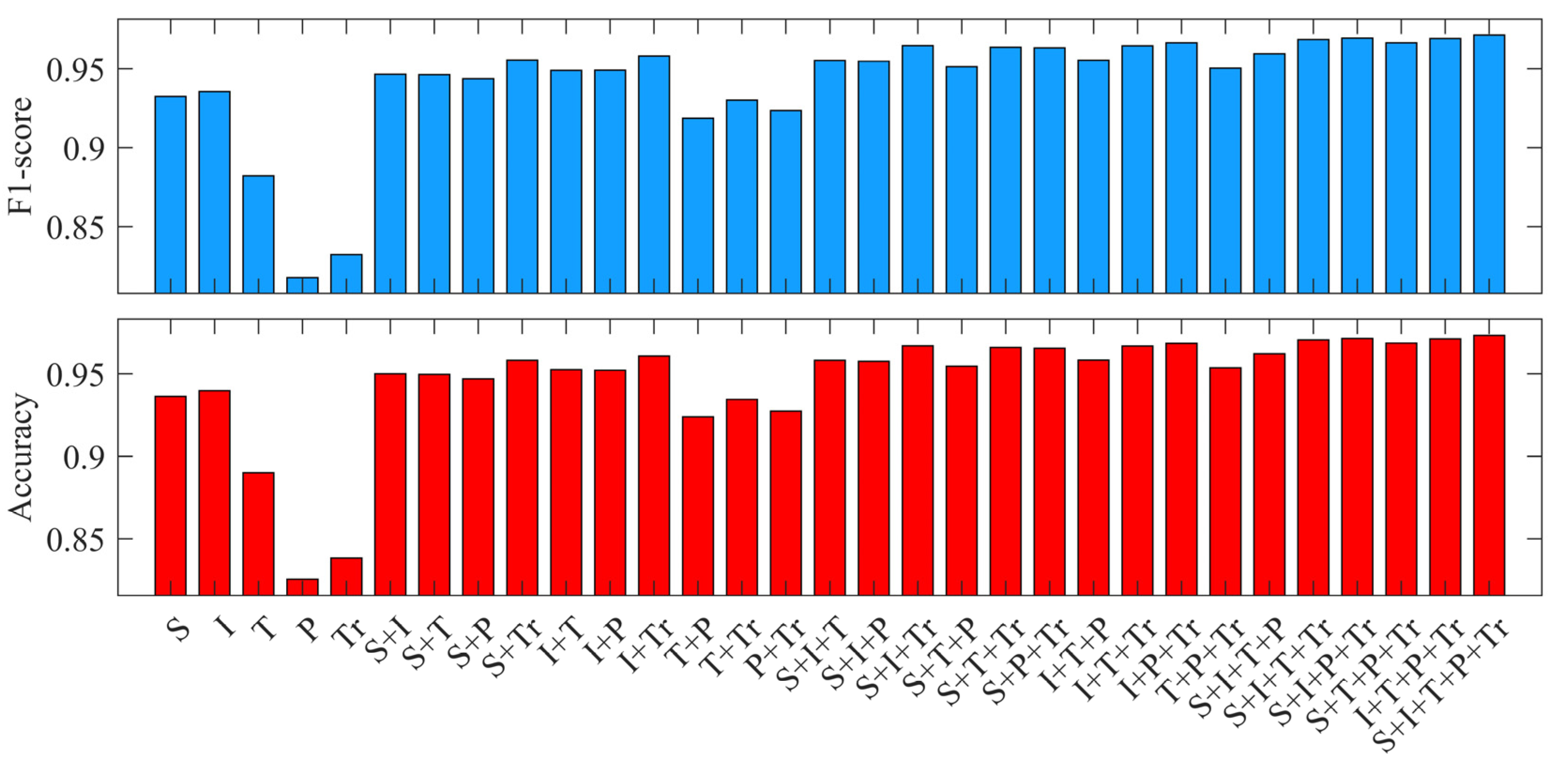
To preliminarily select the optimal feature combination for sandy beach extraction and systematically evaluate the comprehensive extraction performance of different feature combinations across various models, this study constructed a total of 31 feature combinations based on five categories of features. Seven classifiers were trained for each combination, with 100 iterations each, calculating the F1-score and accuracy for every combination under each classifier (Figure 3 and Figure A1, Table A1 and Table A2). The results indicate that when using a single feature category alone, the models generally exhibited lower F1-score and accuracy. The lowest-performing combination was the polarization (P) features, with median F1-score and accuracy averaging only 0.8176 and 0.8255, respectively. After integrating multiple feature types, model performance improved significantly. The combination fusing spectrum, index, terrain, polarization, and texture features (S + I + T + P + Tr) performed best, achieving an F1-score and accuracy of 0.9714 and 0.9733, respectively. These results demonstrate significant differences in classification performance among different feature combinations for sandy beach extraction, with an overall trend that “multi-feature fusion outperforms single features.” The complementarity of multidimensional features plays a positive role in improving the accuracy of sandy beach extraction.

3.2. Multi-Model RFE Results

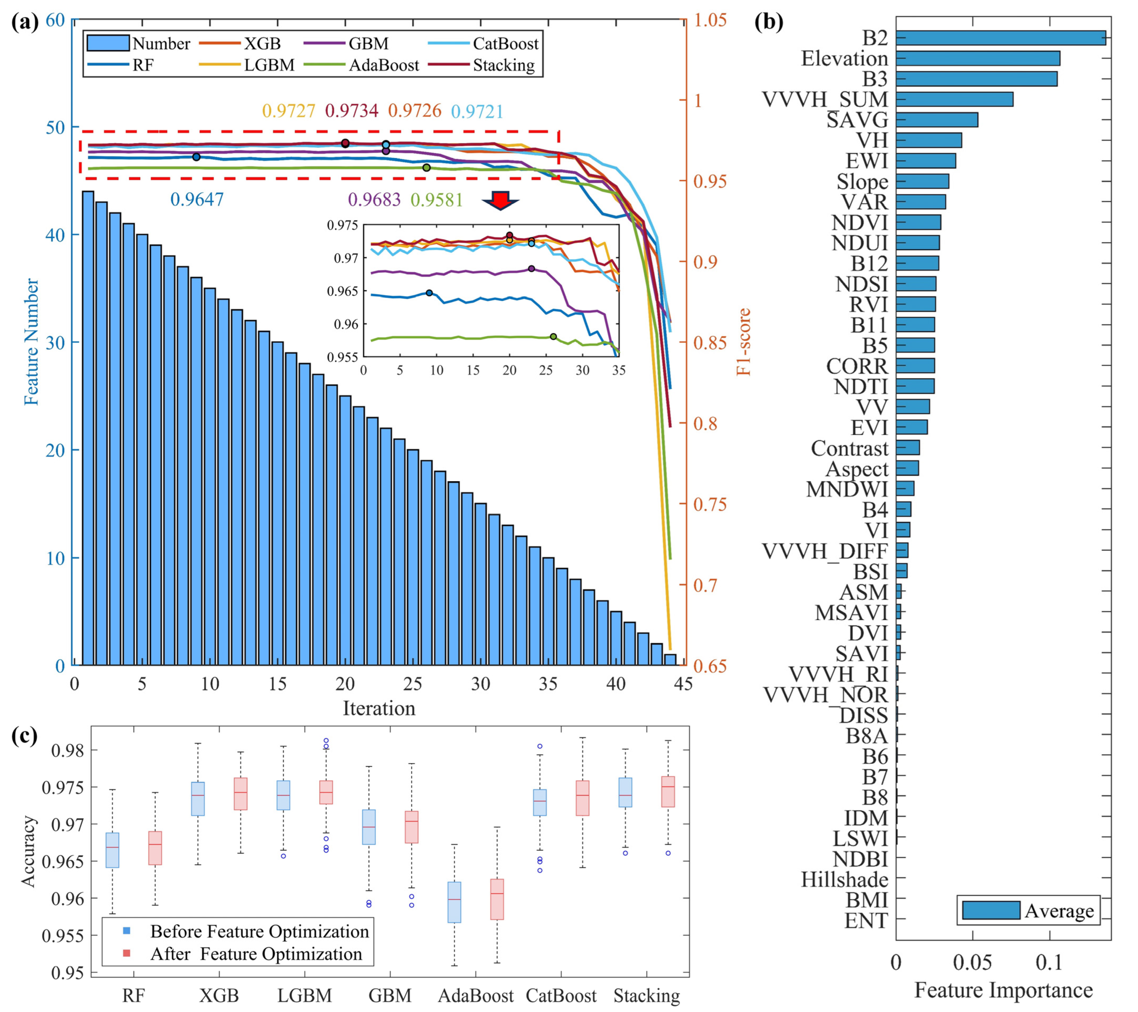
Based on the importance ranking of features in each iteration, a total of 44 rounds of RFE were conducted on the 44 feature variables under the S + I + T + P + Tr scenario (Figure 4a). For the Stacking model, the highest F1-score among the seven models (0.9734) was achieved at the 20th iteration (with 25 features retained). The highest F1-scores for the RF, XGB, LGBM, GBM, AdaBoost, and CatBoost models appeared at the 9th (0.9647), 23rd (0.9726), 20th (0.9727), 23rd (0.9683), 26th (0.9581), and 23rd (0.9721) iterations, respectively. Overall, before the 35th iteration (when only 10 features remained), the F1-score curves of all models fluctuated slightly; after this point, as the number of features further decreased, and model performance rapidly declined, indicating that too few features severely impact the accuracy of sandy beach extraction.
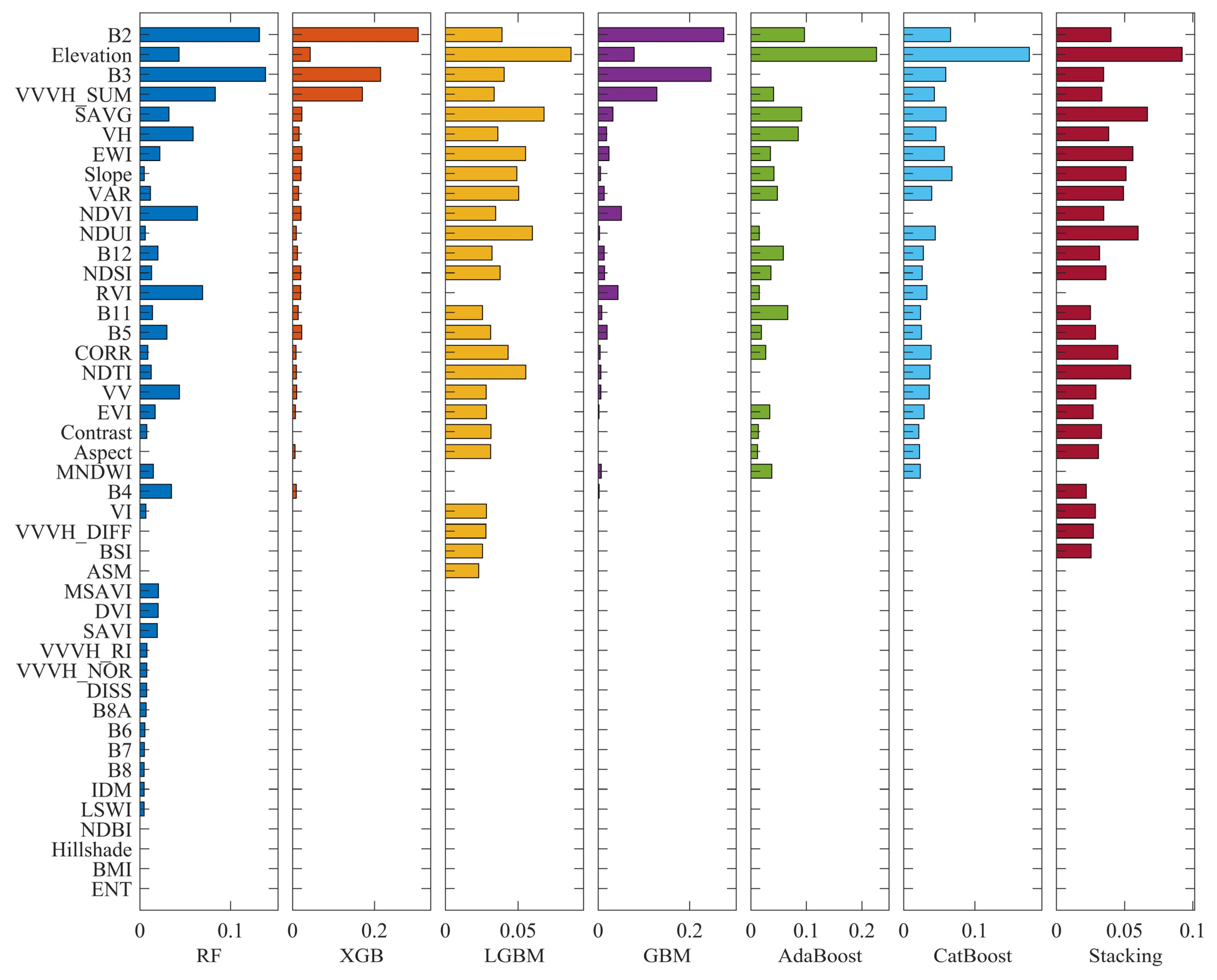
The optimal feature subsets corresponding to the highest F1-scores differed among models (Figure 4b and Figure A2). According to the average importance ranking across the seven models, the top 10 features were B2 (0.1364) > Elevation (0.1067) > B3 (0.1049) > VVVH_SUM (0.0761) > SAVG (0.0532) > VH (0.0426) > EWI (0.0389) > Slope (0.0343) > VAR (0.0323) > NDVI (0.0292). By feature category, spectrum features had the highest average importance (0.1364), followed by terrain features (0.1067), polarization features (0.0761), texture features (0.0532), and index features (0.0389). The most contributing features within each category were B2 (spectrum), Elevation (terrain), VVVH_SUM (polarization), SAVG (texture), and NDVI (index).
This study compared the extraction accuracy of each model before and after feature optimization (Figure 4c and Figure A3). The accuracies of all seven models improved following optimization. In particular, the accuracy increases for RF, XGB, LGBM, GBM, AdaBoost, CatBoost, and Stacking models were 0.04%, 0.04%, 0.04%, 0.08%, 0.08%, 0.08%, and 0.11%, respectively, demonstrating the positive impact of feature optimization on sandy beach extraction accuracy.

3.3. Comparison of Model Results

The study conducted 100 iterations using the optimal feature subset for each model, and the median values of the evaluation metrics were taken as the final accuracy assessment results. The sandy beach extraction performances of all models were compared (Table 4). The Stacking model achieved the highest values in accuracy (0.9750), precision (0.9733), and F1-score (0.9734), while its recall (0.9725) was slightly lower than that of the XGB (0.9733), LGBM (0.9733), and CatBoost (0.9741) models. These results indicate that although the Stacking model does not achieve the highest recall, it demonstrates a strong balance across all evaluation metrics and thus offers the most stable and robust overall performance among the seven models evaluated.
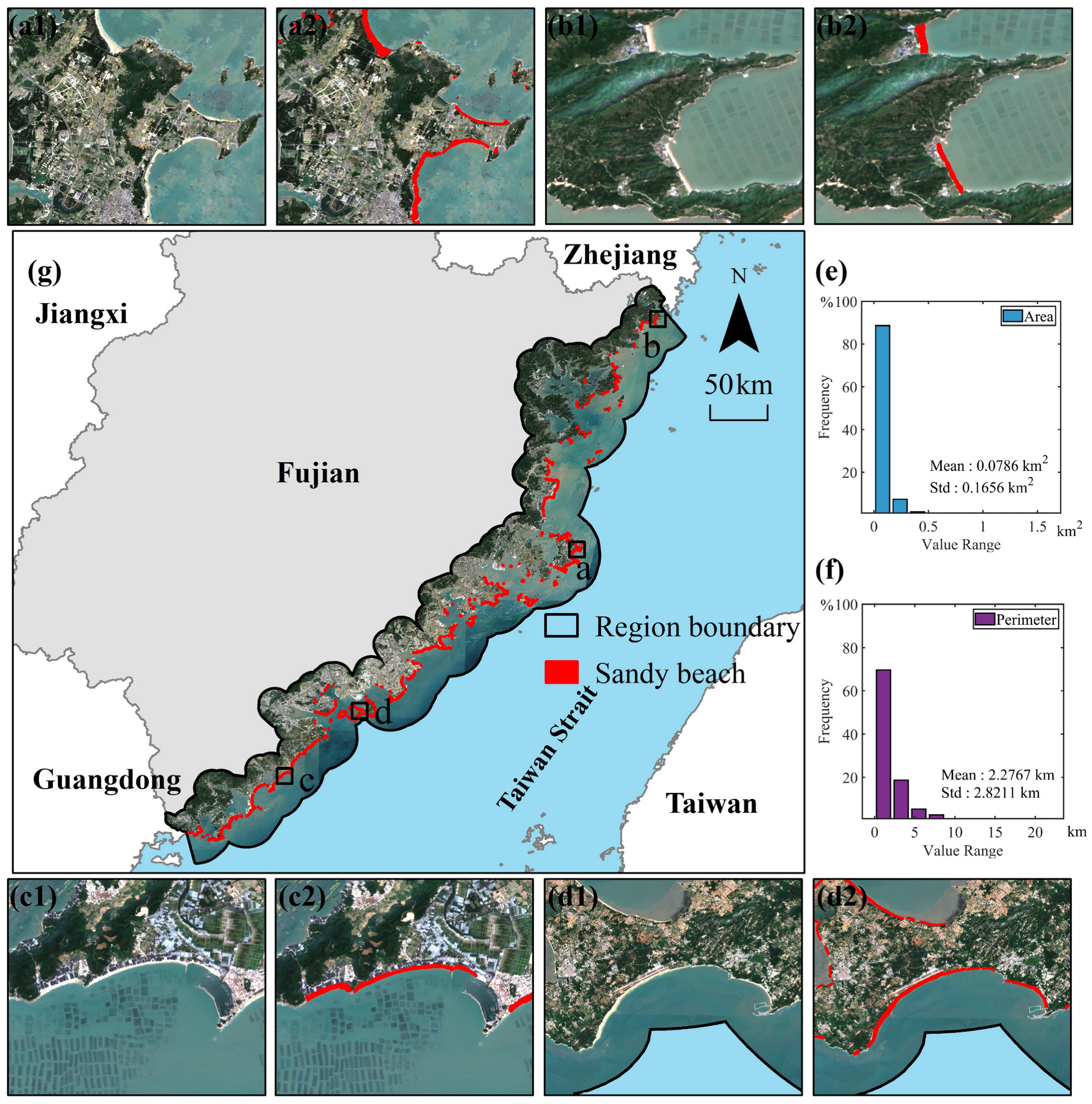
Based on the optimal feature combination of the Stacking model, the spatial distribution and morphological characteristics of sandy beaches in Fujian Province were obtained (Figure 5). A total of 555 sandy beach units were extracted, with a total perimeter of 1263.59 km and a total area of 43.60 km2. The average area of the sandy beaches was 0.0786 km2, with a standard deviation of 0.1656 km2; the average perimeter was 2.2767 km, with a standard deviation of 2.8211 km. The extraction results demonstrate that the sandy beach identification method developed in this study performs excellently in terms of boundary continuity, morphological preservation, and spatial integrity and can accurately characterize the distribution patterns and spatial features of coastal sandy beaches in Fujian.

4. Discussion

4.1. Evolution of Sandy Beach Extraction Strategies: From Spectrum Dominance to Multi-Feature Fusion

In traditional studies on extracting sandy beach information from remote sensing imagery, spectral features have typically served as the core focus. These approaches emphasize selecting appropriate spectral bands and constructing specific spectral indices to characterize the reflectance differences between sandy beaches and surrounding land covers [45,46,47]. Such methods, grounded in spectral response, offer a degree of intuitiveness and operational convenience in practice. They are also well-suited for automation through techniques such as thresholding and supervised classification, which has led to their widespread adoption. However, as a spatially complex and tidally influenced dynamic geomorphic type, the remote sensing characterization of sandy beaches is influenced not only by spectral reflectance but also by a range of factors, including material composition, terrain variation, and polarization response. Especially under complex environmental conditions, relying solely on spectral information may be insufficient to consistently capture the diverse expressions of sandy beach features. Therefore, this study incorporates a broader set of multidimensional feature variables beyond spectrum features (S), including index features (I), polarization features (P), texture features (T), and terrain features (Tr), to construct a more comprehensive feature space. These features aim to characterize the spatial distribution of sandy beaches from multiple perspectives—such as vegetation indices, polarization channel ratios, grayscale texture structures, elevation, and slope. The goal is to explore the complementary roles of different feature dimensions in sandy beach identification. The multi-feature fusion strategy essentially expands the multidimensional interpretation capabilities of remote sensing data. In contrast, previous studies have largely focused on spectral features due in part to the relative ease of data acquisition and the maturity of processing workflows, as well as the developmental stage of remote sensing extraction methodologies [48,49,50,51].

4.2. Analysis of Feature Type Distribution in the Optimal Feature Subset

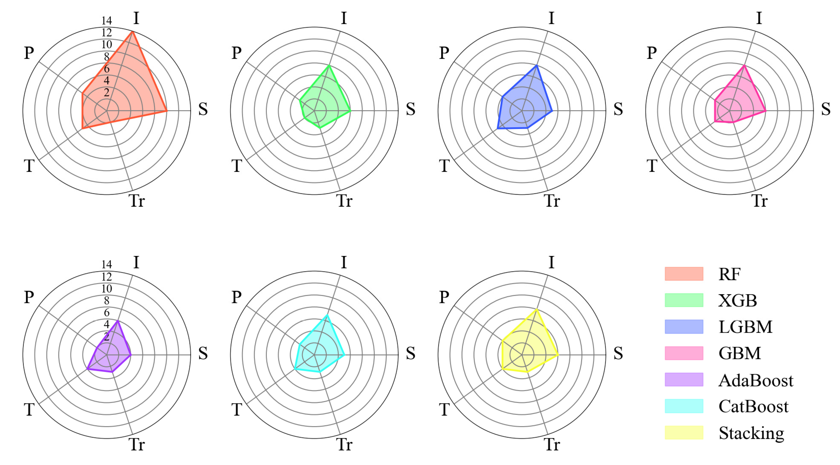
Based on the RFE algorithm, the seven models selected feature subsets with varying proportions of five feature categories (S, I, P, T, Tr), as shown in Figure 6. In terms of quantity, spectral features (S) were still among the most retained categories in most models, particularly in the RF and GBM models, which retained 10 and 6 spectral features, respectively, indicating a relatively high reliance on spectral information during feature selection [52]. Index features (I) were frequently selected across models, with XGB, LGBM, and Stacking each retaining eight index features, suggesting these models are sensitive to index-based variables. The number of polarization, texture, and terrain features remained relatively moderate across models. Notably, AdaBoost, CatBoost, and Stacking preserved more texture and terrain features compared to others, indicating these models may place greater emphasis on auxiliary features during the feature selection process.
By combining the number of features with their importance contributions to model performance, we can further reveal the actual influence of each feature category (Figure 7). Overall, spectrum features contributed the most across most models. In RF and XGB, the importance of spectrum features was approximately 0.39 and 0.58, respectively, with feature counts of 10 and 6. This indicates that spectral features not only dominated in quantity but also played a leading role in model performance [53,54]. Index features were also relatively numerous across models—for example, 14 in RF, 8 in LGBM, and 8 in Stacking. These features showed high importance contributions, around 0.32 in both LGBM and Stacking, suggesting that index features possess both strong predictive power and high information density. Polarization features showed moderate and relatively consistent counts, typically between three and five. Their importance contributions ranged from 0.12 to 0.20, indicating a stable supportive role in the models. Texture and terrain features had the lowest counts, mostly between two and five. However, they exhibited disproportionately high contributions in models such as AdaBoost and CatBoost. For instance, terrain features in AdaBoost and CatBoost contributed as much as 0.28 and 0.27, respectively—far exceeding their numerical share. This suggests that these models are more sensitive to environmental and structural information embedded in terrain and texture features, and effectively utilize them to enhance classification performance.
Overall, significant differences exist among models in terms of feature selection and utilization. On one hand, there is no simple linear relationship between the number of features and their importance contributions; some models are capable of identifying key feature types that are few in number but rich in information, thereby optimizing their weight allocation. On the other hand, models exhibit varying preferences and sensitivities to different feature types, reflecting the distinct responses of model architectures and algorithmic mechanisms to feature characteristics. Spectrum and index features, as the primary sources of information, are generally emphasized across models, while polarization, texture, and terrain features serve as auxiliary yet indispensable complements, further enhancing the models’ representational capacity and generalization performance.

4.3. Comparison of Product Results

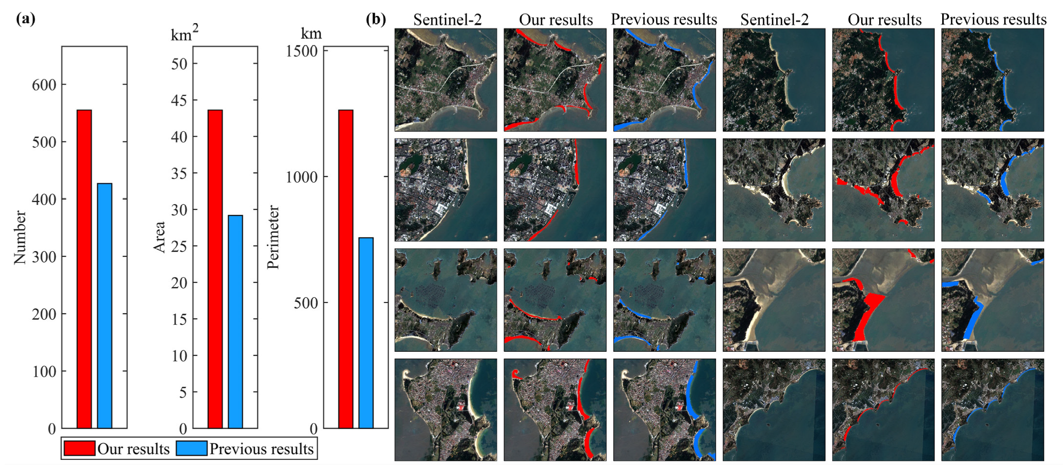
This study builds upon the method of Ni et al. [24] by systematically extending it to enhance the spatial coverage and accuracy of sandy beach identification along the Fujian coastal region. Rather than providing a direct performance comparison, our work supplements their results by incorporating additional sandy beach areas to provide a more comprehensive representation of the coastal geomorphology in Fujian. Compared with the results reported by Ni et al., our approach identified 555 sandy beach units (compared to 427), expanded the total area to 43.60 km2 (compared to 29.17 km2), and increased the total perimeter to 1263.59 km (compared to 756.92 km), demonstrating significant improvements in spatial resolution and boundary detail extraction. The increase in the number of beach units and perimeter length indicates the model’s enhanced ability to capture complex spatial morphologies and fine boundary details, effectively mitigating the loss of critical information caused by excessive merging in conventional approaches.
As illustrated in Figure 8, the proposed method achieves relatively accurate spatial delineation across most areas, though some segmentation errors remain, highlighting opportunities for future refinement. Overall, the primary strengths of this study lie in the application of multi-dimensional feature fusion and optimization strategies, which substantially improve the completeness and accuracy of sandy beach extraction along the Fujian coast. While supplementary processes such as spatial aggregation and boundary optimization contribute to result continuity and robustness, the core driver of the high-quality extraction is the enhanced model performance combined with a rich training dataset. Therefore, this study not only effectively supplements existing methodologies but also provides solid technical support for precise sandy beach identification and subsequent ecological and environmental assessments in the Fujian coastal region.

4.4. Limitations and Future Work

Despite the promising accuracy achieved in sandy beach extraction in this study, several limitations and areas for improvement remain, primarily reflected in the following aspects: (1) This study employs the gray-level co-occurrence matrix (GLCM) to construct texture features based on single-band grayscale images, which enhances the discrimination between sandy beaches and other land cover types to some extent. However, this approach neglects the synergistic texture information across multiple spectral bands, limiting the descriptive power of the texture features. With advances in deep learning and image processing technologies, future research could explore deep texture feature extraction methods based on multispectral image fusion to more comprehensively characterize the microstructural properties of sandy beach surfaces. (2) The training samples used in this study are primarily derived from typical sandy beach areas along the Fujian coast. Although these samples are representative, the coastal types, sandy beach compositions, and anthropogenic activity patterns in Fujian are somewhat limited and may not fully capture the geomorphological diversity of sandy beaches nationally or globally. The generalization capability of the current model in other regions has yet to be systematically validated. To address this, future work plans to construct a comprehensive global sandy beach dataset covering diverse coastal environments to facilitate model retraining and fine-tuning. Additionally, transfer learning and domain adaptation techniques will be considered to improve model applicability across different geographic regions and environmental conditions. Further efforts will include collecting cross-regional datasets to enhance regional robustness and build a more universal sandy beach extraction framework. (3) This study uses the QA60 band provided in the Sentinel-2 Level-2A product for cloud masking due to its operational simplicity and wide adoption in standardized remote sensing workflows. However, QA60 only provides a binary mask for high-confidence opaque clouds and may fail to identify semi-transparent clouds, cloud edges, and shadowed areas, which can result in residual cloud contamination. This contamination may adversely affect model performance, especially under variable atmospheric conditions. Future research could consider replacing QA60 with more advanced cloud masking approaches, such as the Cloud Score+ S2_HARMONIZED V1 dataset, which offers a continuous and probabilistic assessment of cloud and shadow contamination. Such improvements in cloud detection could enhance data quality reliability and further improve model robustness and accuracy, particularly in challenging or transitional weather scenarios. (4) Regarding model performance improvements, the observed increments in evaluation metrics are relatively small. However, in high-accuracy remote sensing classification tasks, especially in complex terrain and spectrally heterogeneous environments, achieving further improvements near saturation is inherently challenging. The sufficient sample size and multi-regional dataset construction have enabled the model to reach a relatively high baseline performance. Hence, even small improvements (e.g., around 0.005) may reflect enhanced model stability in complex boundary scenarios, such as intertidal zones and urban–beach interfaces. The design of 31 feature subsets aimed to systematically evaluate the contribution of different feature combinations and avoid subjective selection. Although this increases computational costs, it provides a foundation for subsequent feature selection and model refinement. Future work will incorporate explainability techniques (e.g., SHAP values) to assist feature selection and verify the influence of sample diversity on model generalization. (5) Beyond technical limitations, natural environmental factors such as tidal dynamics, wave energy, coastal dune systems, estuarine processes, and riverine inputs play critical roles in shaping sandy beach morphology and spectral signatures [55]. These effects are particularly complex in river mouths and estuarine zones, often causing misclassification or reduced extraction accuracy. Future studies could integrate hydrodynamic variables or estuarine classification layers to better distinguish sandy beaches from fluvial or deltaic environments, thus improving extraction accuracy [56]. In summary, while the proposed model demonstrates promising performance in typical coastal areas, improvements remain necessary in feature engineering, cloud masking strategies, sample generalization, and environmental modeling. Addressing these aspects in future research will support the development of a scalable and robust sandy beach extraction framework applicable for large-scale, multi-temporal coastal monitoring.

5. Conclusions

This study constructed a sandy beach extraction feature space based on multi-source remote sensing features and conducted a comparative analysis of sandy beach extraction performance using different feature combinations and multiple classification models. The influence of feature fusion and feature optimization on model performance was comprehensively explored. Based on experimental validation, the following three main conclusions are drawn:
(1)
Among all feature combinations, the fusion of five feature categories—S, I, T, P, and Tr—achieved the best performance, significantly outperforming any single type or partial combination of features. Multidimensional feature fusion effectively compensates for the limitations of individual features, enhances the model’s discrimination capability and robustness, and is a key factor in improving the accuracy of sandy beach extraction.
(2)
Through a multi-model RFE strategy, iterative selection was performed on the five categories of features. The results show that, even with fewer selected key features, the model performance not only remained unaffected but often improved, demonstrating the significant advantage of feature optimization in enhancing both accuracy and computational efficiency. Among the features, spectrum and terrain features ranked highest in importance, particularly mid-band reflectance and elevation information, which played critical roles in model discrimination. Polarization, index, and texture features exhibited strong complementarity across different models. This optimization strategy effectively reduced feature redundancy, improved model generalization and robustness, and provided a reliable foundation for efficient and accurate sandy beach extraction.
(3)
Compared to six other models, the Stacking model, using the optimal feature subset (Elevation, SAVG, NDUI, EWI, NDTI, Slope, VAR, CORR, B2, VH, NDSI, NDVI, B3, VVVH_SUM, Contrast, B12, Aspect, VV, B5, VI, VVVH_DIFF, EVI, BSI, B11, B4), achieved accuracy, precision, recall, and F1-score values of 0.9750, 0.9733, 0.9725, and 0.9734, respectively. This demonstrates its superior comprehensive performance and stability, making it a highly recommended model for large-scale, high-precision sandy beach extraction tasks.

Author Contributions

Conceptualization, J.M. and D.X.; methodology, J.M.; software, Z.T.; validation, Z.T. and J.M.; investigation, J.M. and Q.G.; data curation, J.M.; writing—original draft preparation, J.M.; writing—review and editing, D.X. and Z.T.; visualization, J.M.; project administration, D.X.; funding acquisition, D.X. All authors have read and agreed to the published version of the manuscript.

Funding

This work was funded by the National Key R&D Program of China (grant numbers 2024YFF1308105 and 2024YFF1306301).

Data Availability Statement

The data presented in this study are available on request from the corresponding author.

Acknowledgments

We would like to express our respect and gratitude to the anonymous reviewers and editors for their professional comments and suggestions.

Conflicts of Interest

The authors declare no conflicts of interest.

Appendix A

Table A1. Comprehensive explanation of feature combinations.
Feature CombinationsDescription
SB2, B3, B4, B5, B6, B7, B8, B8A, B11, B12
INDVI, NDSI, NDBI, EVI, SAVI, BSI, NDUI, VI, LSWI, MNDWI, NDTI, RVI, DVI, MSAVI, EWI, BMI
PVV, VH, VVVH_RI, VVVH_DIFF, VVVH_SUM, VVVH_NOR
TASM, Contrast, CORR, DISS, ENT, IDM, SAVG, VAR
TrElevation, Hillshade, Slope, Aspect
S + IB2, B3, B4, B5, B6, B7, B8, B8A, B11, B12, NDVI, NDSI, NDBI, EVI, SAVI, BSI, NDUI, VI, LSWI, MNDWI, NDTI, RVI, DVI, MSAVI, EWI, BMI
S + PB2, B3, B4, B5, B6, B7, B8, B8A, B11, B12, VV, VH, VVVH_RI, VVVH_DIFF, VVVH_SUM, VVVH_NOR
S + TB2, B3, B4, B5, B6, B7, B8, B8A, B11, B12, ASM, Contrast, CORR, DISS, ENT, IDM, SAVG, VAR
S + TrB2, B3, B4, B5, B6, B7, B8, B8A, B11, B12, Elevation, Hillshade, Slope, Aspect
I + PNDVI, NDSI, NDBI, EVI, SAVI, BSI, NDUI, VI, LSWI, MNDWI, NDTI, RVI, DVI, MSAVI, EWI, BMI, VV, VH, VVVH_RI, VVVH_DIFF, VVVH_SUM, VVVH_NOR
I + TNDVI, NDSI, NDBI, EVI, SAVI, BSI, NDUI, VI, LSWI, MNDWI, NDTI, RVI, DVI, MSAVI, EWI, BMI, ASM, Contrast, CORR, DISS, ENT, IDM, SAVG, VAR
I + TrNDVI, NDSI, NDBI, EVI, SAVI, BSI, NDUI, VI, LSWI, MNDWI, NDTI, RVI, DVI, MSAVI, EWI, BMI, Elevation, Hillshade, Slope, Aspect
P + TVV, VH, VVVH_RI, VVVH_DIFF, VVVH_SUM, VVVH_NOR, ASM, Contrast, CORR, DISS, ENT, IDM, SAVG, VAR
P + TrVV, VH, VVVH_RI, VVVH_DIFF, VVVH_SUM, VVVH_NOR, Elevation, Hillshade, Slope, Aspect
T + TrASM, Contrast, CORR, DISS, ENT, IDM, SAVG, VAR, Elevation, Hillshade, Slope, Aspect
S + I + PB2, B3, B4, B5, B6, B7, B8, B8A, B11, B12, NDVI, NDSI, NDBI, EVI, SAVI, BSI, NDUI, VI, LSWI, MNDWI, NDTI, RVI, DVI, MSAVI, EWI, BMI, VV, VH, VVVH_RI, VVVH_DIFF, VVVH_SUM, VVVH_NOR
S + I + TB2, B3, B4, B5, B6, B7, B8, B8A, B11, B12, NDVI, NDSI, NDBI, EVI, SAVI, BSI, NDUI, VI, LSWI, MNDWI, NDTI, RVI, DVI, MSAVI, EWI, BMI, ASM, Contrast, CORR, DISS, ENT, IDM, SAVG, VAR
S + I + TrB2, B3, B4, B5, B6, B7, B8, B8A, B11, B12, NDVI, NDSI, NDBI, EVI, SAVI, BSI, NDUI, VI, LSWI, MNDWI, NDTI, RVI, DVI, MSAVI, EWI, BMI, Elevation, Hillshade, Slope, Aspect
S + P + TB2, B3, B4, B5, B6, B7, B8, B8A, B11, B12, VV, VH, VVVH_RI, VVVH_DIFF, VVVH_SUM, VVVH_NOR, ASM, Contrast, CORR, DISS, ENT, IDM, SAVG, VAR
S + P + TrB2, B3, B4, B5, B6, B7, B8, B8A, B11, B12, VV, VH, VVVH_RI, VVVH_DIFF, VVVH_SUM, VVVH_NOR, Elevation, Hillshade, Slope, Aspect
S + T + TrB2, B3, B4, B5, B6, B7, B8, B8A, B11, B12, ASM, Contrast, CORR, DISS, ENT, IDM, SAVG, VAR, Elevation, Hillshade, Slope, Aspect
I + P + TNDVI, NDSI, NDBI, EVI, SAVI, BSI, NDUI, VI, LSWI, MNDWI, NDTI, RVI, DVI, MSAVI, EWI, BMI, VV, VH, VVVH_RI, VVVH_DIFF, VVVH_SUM, VVVH_NOR, ASM, Contrast, CORR, DISS, ENT, IDM, SAVG, VAR
I + P + TrNDVI, NDSI, NDBI, EVI, SAVI, BSI, NDUI, VI, LSWI, MNDWI, NDTI, RVI, DVI, MSAVI, EWI, BMI, VV, VH, VVVH_RI, VVVH_DIFF, VVVH_SUM, VVVH_NOR, Elevation, Hillshade, Slope, Aspect
I + T + TrNDVI, NDSI, NDBI, EVI, SAVI, BSI, NDUI, VI, LSWI, MNDWI, NDTI, RVI, DVI, MSAVI, EWI, BMI, ASM, Contrast, CORR, DISS, ENT, IDM, SAVG, VAR, Elevation, Hillshade, Slope, Aspect
P + T + TrVV, VH, VVVH_RI, VVVH_DIFF, VVVH_SUM, VVVH_NOR, ASM, Contrast, CORR, DISS, ENT, IDM, SAVG, VAR, Elevation, Hillshade, Slope, Aspect
S + I + P + TB2, B3, B4, B5, B6, B7, B8, B8A, B11, B12, NDVI, NDSI, NDBI, EVI, SAVI, BSI, NDUI, VI, LSWI, MNDWI, NDTI, RVI, DVI, MSAVI, EWI, BMI, VV, VH, VVVH_RI, VVVH_DIFF, VVVH_SUM, VVVH_NOR, ASM, Contrast, CORR, DISS, ENT, IDM, SAVG, VAR
S + I + P + TrB2, B3, B4, B5, B6, B7, B8, B8A, B11, B12, NDVI, NDSI, NDBI, EVI, SAVI, BSI, NDUI, VI, LSWI, MNDWI, NDTI, RVI, DVI, MSAVI, EWI, BMI, VV, VH, VVVH_RI, VVVH_DIFF, VVVH_SUM, VVVH_NOR, Elevation, Hillshade, Slope, Aspect
S + I + T + TrB2, B3, B4, B5, B6, B7, B8, B8A, B11, B12, NDVI, NDSI, NDBI, EVI, SAVI, BSI, NDUI, VI, LSWI, MNDWI, NDTI, RVI, DVI, MSAVI, EWI, BMI, ASM, Contrast, CORR, DISS, ENT, IDM, SAVG, VAR, Elevation, Hillshade, Slope, Aspect
S + P + T + TrB2, B3, B4, B5, B6, B7, B8, B8A, B11, B12, VV, VH, VVVH_RI, VVVH_DIFF, VVVH_SUM, VVVH_NOR, ASM, Contrast, CORR, DISS, ENT, IDM, SAVG, VAR, Elevation, Hillshade, Slope, Aspect
I + P + T + TrNDVI, NDSI, NDBI, EVI, SAVI, BSI, NDUI, VI, LSWI, MNDWI, NDTI, RVI, DVI, MSAVI, EWI, BMI, VV, VH, VVVH_RI, VVVH_DIFF, VVVH_SUM, VVVH_NOR, ASM, Contrast, CORR, DISS, ENT, IDM, SAVG, VAR, Elevation, Hillshade, Slope, Aspect
S + I + P + T + TrB2, B3, B4, B5, B6, B7, B8, B8A, B11, B12, NDVI, NDSI, NDBI, EVI, SAVI, BSI, NDUI, VI, LSWI, MNDWI, NDTI, RVI, DVI, MSAVI, EWI, BMI, VV, VH, VVVH_RI, VVVH_DIFF, VVVH_SUM, VVVH_NOR, ASM, Contrast, CORR, DISS, ENT, IDM, SAVG, VAR, Elevation, Hillshade, Slope, Aspect
Table A2. Median accuracy of different models across feature combinations.
Feature CombinationsRFXGBLGBMGBMAdaBoostCatBoostStacking
S0.93830.94020.94020.93340.92360.93790.9410
I0.94050.94430.94510.93720.92220.94340.9459
P0.88820.88590.89150.89110.88680.89300.8935
T0.82560.81800.82730.82810.81800.83030.8310
Tr0.82570.83760.83950.84110.83970.84210.8422
S + I0.94810.95360.95410.94650.94060.95280.9544
S + P0.95140.95280.95320.94590.93910.95110.9547
S + T0.94800.95050.95110.94240.93560.94840.9525
S + Tr0.95730.96180.96150.95550.95210.95750.9621
I + P0.95030.95630.95690.95030.94090.95500.9580
I + T0.95110.95580.95690.94890.93970.95540.9577
I + Tr0.95520.96520.96510.95660.95290.96490.9659
P + T0.92360.92160.92550.92480.91780.92700.9272
P + Tr0.93220.93350.93650.93450.93090.93640.9375
T + Tr0.92740.92680.93070.92870.91700.93020.9313
S + I + P0.95690.96150.96210.95550.94980.96000.9621
S + I + T0.95470.96100.96160.95440.94960.96000.9616
S + I + Tr0.96120.96970.97000.96480.96290.96940.9708
S + P + T0.95300.95800.95820.95030.94530.95770.9596
S + P + Tr0.96360.96830.96860.96450.96010.96780.9689
S + T + Tr0.96260.96780.96720.96310.96080.96810.9692
I + P + T0.95580.96160.96210.95580.94990.96040.9626
I + P + Tr0.96180.97000.97010.96590.96160.96930.9700
I + T + Tr0.96340.97190.97120.96670.96370.97110.9719
P + T + Tr0.95000.95470.95600.95360.94840.95580.9566
S + I + P + T0.95990.96560.96600.95930.95480.96380.9660
S + I + P + Tr0.96550.97320.97380.96900.96570.97310.9738
S + I + T + Tr0.96590.97430.97470.96930.96700.97380.9752
S + P + T + Tr0.96520.97090.97090.96710.96410.97040.9722
I + P + T + Tr0.96530.97430.97490.96860.96700.97350.9746
S + I + P + T + Tr0.96810.97600.97600.97160.96970.97540.9762
Table A3. Median F1-score of different models across feature combinations.
Feature CombinationsRFXGBLGBMGBMAdaBoostCatBoostStacking
S0.93430.93620.93630.92950.91930.93420.9372
I0.93620.94040.94120.93340.91680.93950.9421
P0.88040.87810.88360.88390.87780.88540.8859
T0.81670.80940.81960.82200.81070.82250.8227
Tr0.82190.83170.83350.83470.83380.83580.8347
S + I0.94460.95030.95090.94320.93630.94940.9511
S + P0.94790.94950.94980.94230.93530.94770.9512
S + T0.94470.94720.94810.93930.93210.94530.9495
S + Tr0.95440.95900.95900.95260.94930.95480.9594
I + P0.94640.95320.95370.94670.93690.95180.9548
I + T0.94790.95300.95410.94570.93590.95250.9549
I + Tr0.95210.96270.96260.95360.94970.96250.9635
P + T0.91790.91700.92050.91980.91150.92200.9220
P + Tr0.92740.92950.93220.93050.92640.93220.9332
T + Tr0.92350.92280.92710.92510.91180.92680.9277
S + I + P0.95360.95870.95920.95240.94640.95730.9593
S + I + T0.95170.95820.95910.95140.94620.95720.9591
S + I + Tr0.95850.96760.96800.96240.96040.96730.9687
S + P + T0.94970.95510.95530.94700.94150.95480.9565
S + P + Tr0.96080.96600.96630.96210.95720.96570.9668
S + T + Tr0.96010.96570.96500.96080.95820.96600.9670
I + P + T0.95250.95890.95930.95280.94650.95790.9598
I + P + Tr0.95870.96790.96810.96360.95890.96710.9678
I + T + Tr0.96080.97000.96930.96450.96120.96920.9701
P + T + Tr0.94650.95190.95300.95040.94480.95280.9534
S + I + P + T0.95680.96310.96350.95630.95150.96140.9636
S + I + P + Tr0.96270.97140.97200.96690.96350.97130.9720
S + I + T + Tr0.96340.97260.97310.96730.96460.97210.9735
S + P + T + Tr0.96260.96900.96890.96470.96180.96840.9703
I + P + T + Tr0.96270.97260.97320.96650.96480.97170.9729
S + I + P + T + Tr0.96570.97430.97440.96950.96770.97370.9746
Figure A1. Mean of median F1-Score and accuracy of seven models across different feature combinations.
Remotesensing 17 02754 g0a1
Figure A2. Feature importance rankings across seven models.
Remotesensing 17 02754 g0a2
Figure A3. Performance comparison of seven models before and after feature optimization.
Remotesensing 17 02754 g0a3

References

  1. Zhou, Z.; Wei, Y.; Geng, L.; Zhang, Y.; Gu, Y.; Finotello, A.; D’Alpaos, A.; Gong, Z.; Xu, F.; Zhang, C.; et al. Cross-Shore Parallel Tidal Channel Systems Formed by Alongshore Currents. Nat. Commun. 2024, 15, 4732. [Google Scholar] [CrossRef]
  2. Bozzeda, F.; Ortega, L.; Costa, L.L.; Fanini, L.; Barboza, C.A.M.; McLachlan, A.; Defeo, O. Global Patterns in Sandy Beach Erosion: Unraveling the Roles of Anthropogenic, Climatic and Morphodynamic Factors. Front. Mar. Sci. 2023, 10, 1270490. [Google Scholar] [CrossRef]
  3. Lansu, E.M.; Reijers, V.C.; Höfer, S.; Luijendijk, A.; Rietkerk, M.; Wassen, M.J.; Lammerts, E.J.; van der Heide, T. A Global Analysis of How Human Infrastructure Squeezes Sandy Coasts. Nat. Commun. 2024, 15, 432. [Google Scholar] [CrossRef]
  4. Mentaschi, L.; Vousdoukas, M.I.; Pekel, J.-F.; Voukouvalas, E.; Feyen, L. Global Long-Term Observations of Coastal Erosion and Accretion. Sci. Rep. 2018, 8, 12876. [Google Scholar] [CrossRef] [PubMed]
  5. Yuan, R.; Xu, R.; Zhang, H.; Hua, Y.; Zhang, H.; Zhong, X.; Chen, S. Detecting Shoreline Changes on the Beaches of Hainan Island (China) for the Period 2013–2023 Using Multi-Source Data. Water 2024, 16, 1034. [Google Scholar] [CrossRef]
  6. Sekar, C.S.; Kankara, R.S.; Kalaivanan, P. Pixel-Based Classification Techniques for Automated Shoreline Extraction on Open Sandy Coast Using Different Optical Satellite Images. Arab. J. Geosci. 2022, 15, 939. [Google Scholar] [CrossRef]
  7. Bao, Z.; Sha, J.; Li, X.; Hanchiso, T.; Shifaw, E. Monitoring of Beach Litter by Automatic Interpretation of Unmanned Aerial Vehicle Images Using the Segmentation Threshold Method. Mar. Pollut. Bull. 2018, 137, 388–398. [Google Scholar] [CrossRef]
  8. Zhu, Y.; Li, Z.; Zhao, Z.; Lu, L.; Yang, S.; Wang, Z. Spatio-Temporal Changes of Coastline in Jiaozhou Bay from 1987 to 2022 Based on Optical and SAR Data. Front. Mar. Sci. 2023, 10, 1233410. [Google Scholar] [CrossRef]
  9. Wu, J.; Li, Y.; Zhong, B.; Zhang, Y.; Liu, Q.; Shi, X.; Ji, C.; Wu, S.; Sun, B.; Li, C.; et al. Synergistic Coupling of Multi-Source Remote Sensing Data for Sandy Land Detection and Multi-Indicator Integrated Evaluation. Remote Sens. 2024, 16, 4322. [Google Scholar] [CrossRef]
  10. Wang, Z.; Fang, Z.; Chang, J.; Wang, Z.; Shen, W. A Two-Step Approach to Extracting Sandy Beaches Through Integrating Spatial Semantic Information from Open-Source Geospatial Datasets. Trans. GIS 2024, 28, 2379–2396. [Google Scholar] [CrossRef]
  11. Hu, L.; Xu, N.; Liang, J.; Li, Z.; Chen, L.; Zhao, F. Advancing the Mapping of Mangrove Forests at National-Scale Using Sentinel-1 and Sentinel-2 Time-Series Data with Google Earth Engine: A Case Study in China. Remote Sens. 2020, 12, 3120. [Google Scholar] [CrossRef]
  12. Xu, N.; Wang, L.; Xu, H.; Ma, Y.; Li, Y.; Wang, X.H. Deriving Accurate Intertidal Topography for Sandy Beaches Using ICESat-2 Data and Sentinel-2 Imagery. Remote Sens. 2024, 16, 305. [Google Scholar] [CrossRef]
  13. Sun, S.; Xue, Q.; Xing, X.; Zhao, H.; Zhang, F. Remote Sensing Image Interpretation for Coastal Zones: A Review. Remote Sens. 2024, 16, 4701. [Google Scholar] [CrossRef]
  14. Hu, F.; Li, Y.; Liang, J.; Li, Z.; Xie, M.; Chen, X.; Xiao, Z. History of Coastal Dune Evolution in the Fujian Region of Southeastern China over the Last Millennium. Mar. Geol. 2022, 451, 106878. [Google Scholar] [CrossRef]
  15. Jin, J.; Li, Z.; Jiang, F.; Deng, T.; Hu, F.; Ling, Z. Coastal Environment of the Past Millennium Recorded by a Coastal Dune in Fujian, China. J. Arid Land 2016, 8, 707–721. [Google Scholar] [CrossRef]
  16. Li, M.; Chen, B.; Webster, C.; Gong, P.; Xu, B. The landea interface mapping: China’s coastal land covers at 10 m for 2020. Sci. Bull. 2022, 67, 1750–1754. [Google Scholar] [CrossRef] [PubMed]
  17. DeVries, B.; Huang, C.; Armston, J.; Huang, W.; Jones, J.W.; Lang, M.W. Rapid and robust monitoring of flood events using Sentinel-1 and Landsat data on the Google Earth Engine. Remote Sens. Environ. 2020, 240, 111664. [Google Scholar] [CrossRef]
  18. Yao, S.; Tan, K.; Wang, Y.; Zhang, W.; Liu, S.; Yang, J. Estimating terrain elevations at 10 m resolution by integrating random forest machine learning model and ICESat-2, Sentinel-1, and Sentinel-2 satellite remotely sensed data. Int. J. Appl. Earth Obs. Geoinf. 2024, 132, 104010. [Google Scholar] [CrossRef]
  19. Ezimand, K.; Aghighi, H.; Ashourloo, D.; Shakiba, A. The Analysis of the Spatio-Temporal Changes and Prediction of Built-Up Lands and Urban Heat Islands Using Multi-Temporal Satellite Imagery. Sustain. Cities Soc. 2024, 103, 105231. [Google Scholar] [CrossRef]
  20. Zhang, M.; Tan, S.; Zhang, C.; Han, S.; Zou, S.; Chen, E. Assessing the Impact of Fractional Vegetation Cover on Urban Thermal Environment: A Case Study of Hangzhou, China. Sustain. Cities Soc. 2023, 96, 104663. [Google Scholar] [CrossRef]
  21. Jia, M.; Wang, Z.; Mao, D.; Ren, C.; Wang, C.; Wang, Y. Rapid, Robust, and Automated Mapping of Tidal Flats in China Using Time Series Sentinel-2 Images and Google Earth Engine. Remote Sens. Environ. 2021, 255, 112285. [Google Scholar] [CrossRef]
  22. Li, H.; Jia, M.; Zhang, R.; Ren, Y.; Wen, X. Incorporating the Plant Phenological Trajectory into Mangrove Species Mapping with Dense Time Series Sentinel-2 Imagery and the Google Earth Engine Platform. Remote Sens. 2019, 11, 2479. [Google Scholar] [CrossRef]
  23. Lv, T.; Hu, H.; Han, H.; Zhang, X.; Fan, H.; Yan, K. Towards sustainability: The spatiotemporal patterns and influence mechanism of urban sprawl intensity in the Yangtze River Delta urban agglomeration. Habitat Int. 2024, 148, 103089. [Google Scholar] [CrossRef]
  24. Ni, M.; Xu, N.; Ou, Y.; Yao, J.; Li, Z.; Mo, F.; Huang, C.; Xin, H.; Xu, H. The first 10-m China’s national-scale sandy beach map in 2022 derived from Sentinel-2 imagery. Int. J. Digit. Earth 2024, 17, 2425163. [Google Scholar] [CrossRef]
  25. Luijendijk, A.; Hagenaars, G.; Ranasinghe, R.; Baart, F.; Donchyts, G.; Aarninkhof, S. The State of the World’s Beaches. Sci. Rep. 2018, 8, 6641. [Google Scholar] [CrossRef]
  26. Yin, Z.; Wu, P.; Li, X.; Hao, Z.; Ma, X.; Fan, R.; Liu, C.; Ling, F. Super-Resolution Water Body Mapping with a Feature Collaborative CNN Model by Fusing Sentinel-1 and Sentinel-2 Images. Int. J. Appl. Earth Obs. Geoinf. 2024, 134, 104176. [Google Scholar] [CrossRef]
  27. Zheng, Y.; Tang, L.; Wang, H. An Improved Approach for Monitoring Urban Built-Up Areas by Combining NPP-VIIRS Nighttime Light, NDVI, NDWI, and NDBI. J. Clean. Prod. 2021, 328, 129488. [Google Scholar] [CrossRef]
  28. Xiao, X.; Liang, S. Assessment of Snow Cover Mapping Algorithms from Landsat Surface Reflectance Data and Application to Automated Snowline Delineation. Remote Sens. Environ. 2024, 307, 114163. [Google Scholar] [CrossRef]
  29. Muhaimin, M.; Fitriani, D.; Adyatma, S.; Arisanty, D. Mapping Build-Up Area Density Using Normalized Difference Built-Up Index (NDBI) and Urban Index (UI) Wetland in the City Banjarmasin. IOP Conf. Ser. Earth Environ. Sci. 2022, 1089, 012036. [Google Scholar] [CrossRef]
  30. Wang, G.; Peng, W.; Zhang, L.; Zhang, J.; Xiang, J. Vegetation EVI Changes and Response to Natural Factors and Human Activities Based on Geographically and Temporally Weighted Regression. Glob. Ecol. Conserv. 2023, 45, e02531. [Google Scholar] [CrossRef]
  31. Xu, H.; Chen, J.; He, G.; Lin, Z.; Bai, Y.; Ren, M.; Zhang, H.; Yin, H.; Liu, F. Immediate Assessment of Forest Fire Using a Novel Vegetation Index and Machine Learning Based on Multi-Platform, High Temporal Resolution Remote Sensing Images. Int. J. Appl. Earth Obs. Geoinf. 2024, 134, 104210. [Google Scholar] [CrossRef]
  32. Ni, R.; Tian, J.; Li, X.; Yin, D.; Li, J.; Gong, H.; Zhang, J.; Zhu, L.; Wu, D. An Enhanced Pixel-Based Phenological Feature for Accurate Paddy Rice Mapping with Sentinel-2 Imagery in Google Earth Engine. ISPRS J. Photogramm. Remote Sens. 2021, 178, 282–296. [Google Scholar] [CrossRef]
  33. Zhang, Q.; Li, B.; Thau, D.; Moore, R. Building a Better Urban Picture: Combining Day and Night Remote Sensing Imagery. Remote Sens. 2015, 7, 11887–11913. [Google Scholar] [CrossRef]
  34. He, Y.; Zhang, B.; Ma, C. The Impact of Dynamic Change of Cropland on Grain Production in Jilin. J. Geogr. Sci. 2004, 14 (Suppl. S1), 56–62. [Google Scholar] [CrossRef]
  35. Chandrasekar, K.; Sesha Sai, M.V.R.; Roy, P.S.; Dwevedi, R.S. Land Surface Water Index (LSWI) Response to Rainfall and NDVI Using the MODIS Vegetation Index Product. Int. J. Remote Sens. 2010, 31, 3987–4005. [Google Scholar] [CrossRef]
  36. Tellman, B.; Sullivan, J.A.; Kuhn, C.; Kettner, A.J.; Doyle, C.S.; Brakenridge, G.R.; Erickson, T.A.; Slayback, D.A. Satellite Imaging Reveals Increased Proportion of Population Exposed to Floods. Nature 2021, 596, 80–86. [Google Scholar] [CrossRef] [PubMed]
  37. Fernández-Buces, N.; Siebe, C.; Cram, S.; Palacio, J.L. Mapping Soil Salinity Using a Combined Spectral Response Index for Bare Soil and Vegetation: A Case Study in the Former Lake Texcoco, Mexico. J. Arid Environ. 2006, 65, 644–667. [Google Scholar] [CrossRef]
  38. Li, C.; Lin, L.; Hao, Z.; Post, C.J.; Chen, Z.; Liu, J.; Yu, K. Developing a USLE Cover and Management Factor (C) for Forested Regions of Southern China. Front. Earth Sci. 2020, 14, 660–672. [Google Scholar] [CrossRef]
  39. Zhang, Y.; Wang, Y.; Ding, N.; Yang, X. Assessing the Contributions of Urban Green Space Indices and Spatial Structure in Mitigating Urban Thermal Environment. Remote Sens. 2023, 15, 2414. [Google Scholar] [CrossRef]
  40. Wang, S.; Baig, M.H.A.; Zhang, L.; Jiang, H.; Ji, Y.; Zhao, H.; Tian, J. A Simple Enhanced Water Index (EWI) for Percent Surface Water Estimation Using Landsat Data. IEEE J. Sel. Top. Appl. Earth Obs. Remote Sens. 2015, 8, 90–97. [Google Scholar] [CrossRef]
  41. Wang, R.; Qi, H.; Cai, F.; Yin, H.; Liu, G.; Zhao, S. Research on Beach Morphology Extraction Method Based on Beach Morphology Index. Mar. Bull. 2024, 43, 97–105. [Google Scholar]
  42. Jiang, W.; Tian, B.; Duan, Y.; Chen, C.; Hu, Y. Rapid Mapping and Spatial Analysis on the Distribution of Photovoltaic Power Stations with Sentinel-1 & 2 Images in Chinese Coastal Provinces. Int. J. Appl. Earth Obs. Geoinf. 2023, 118, 103280. [Google Scholar]
  43. Wang, L.; Wang, J.; Zhang, X.; Wang, L.; Qin, F. Deep Segmentation and Classification of Complex Crops Using Multi-Feature Satellite Imagery. Comput. Electron. Agric. 2022, 200, 107249. [Google Scholar] [CrossRef]
  44. Lin, J.; Jin, X.; Ren, J.; Liu, J.; Liang, X.; Zhou, Y. Rapid Mapping of Large-Scale Greenhouse Based on Integrated Learning Algorithm and Google Earth Engine. Remote Sens. 2021, 13, 1245. [Google Scholar] [CrossRef]
  45. Quartel, S.; Addink, E.A.; Ruessink, B.G. Object-Oriented Extraction of Beach Morphology from Video Images. Int. J. Appl. Earth Obs. Geoinf. 2006, 8, 256–269. [Google Scholar] [CrossRef]
  46. Sozio, A.; Scarrica, V.M.; Rizzo, A.; Aucelli, P.P.C.; Barracane, G.; Dimuccio, L.A.; Ferreira, R.; La Salandra, M.; Staiano, A.; Tarantino, M.P.; et al. Application of Direct and Indirect Methodologies for Beach Litter Detection in Coastal Environments. Remote Sens. 2024, 16, 3617. [Google Scholar] [CrossRef]
  47. Yin, H.; Cai, F.; Qi, H.; Jiang, Y.; Liu, G.; Cao, Z.; Sun, Y.; Xiao, Z. Analysis of Tidal Cycle Wave Breaking Distribution Characteristics on a Low-Tide Terrace Beach Using Video Imagery Segmentation. Remote Sens. 2024, 16, 4616. [Google Scholar] [CrossRef]
  48. Chen, Z.; Zhang, H.; Zhang, M.; Wu, Y.; Liu, Y. Mangrove Mapping in China Using Gaussian Mixture Model with a Novel Mangrove Index (SSMI) Derived from Optical and SAR Imagery. ISPRS J. Photogramm. Remote Sens. 2024, 218, 466–486. [Google Scholar] [CrossRef]
  49. Tian, P.; Liu, Y.; Li, J.; Pu, R.; Cao, L.; Zhang, H.; Ai, S.; Yang, Y. Mapping Coastal Aquaculture Ponds of China Using Sentinel SAR Images in 2020 and Google Earth Engine. Remote Sens. 2022, 14, 5372. [Google Scholar] [CrossRef]
  50. Mao, Y.; Harris, D.L.; Xie, Z.; Phinn, S. Global Coastal Geomorphology—Integrating Earth Observation and Geospatial Data. Remote Sens. Environ. 2022, 278, 113082. [Google Scholar] [CrossRef]
  51. Zhao, C.; Qin, C.-Z. 10-m-Resolution Mangrove Maps of China Derived from Multi-Source and Multi-Temporal Satellite Observations. ISPRS J. Photogramm. Remote Sens. 2020, 169, 389–405. [Google Scholar] [CrossRef]
  52. Belgiu, M.; Drăguţ, L. Random Forest in Remote Sensing: A Review of Applications and Future Directions. ISPRS J. Photogramm. Remote Sens. 2016, 114, 24–31. [Google Scholar] [CrossRef]
  53. Chen, B.; Huang, B.; Xu, B. Multi-Source Remotely Sensed Data Fusion for Improving Land Cover Classification. ISPRS J. Photogramm. Remote Sens. 2017, 124, 27–39. [Google Scholar] [CrossRef]
  54. Shirmard, H.; Farahbakhsh, E.; Müller, R.D.; Chandra, R. A Review of Machine Learning in Processing Remote Sensing Data for Mineral Exploration. Remote Sens. Environ. 2022, 268, 112750. [Google Scholar] [CrossRef]
  55. Talke, S.A. How Tidal Properties Influence the Future Duration of Coastal Flooding. npj Nat. Hazards 2025, 2, 36. [Google Scholar] [CrossRef]
  56. Zhou, Z.; Liang, M.; Chen, L.; Xu, M.; Chen, X.; Geng, L.; Li, H.; Serrano, D.; Zhang, H.; Gong, Z.; et al. Processes, Feedbacks, and Morphodynamic Evolution of Tidal Flat–Marsh Systems: Progress and Challenges. Water Sci. Eng. 2022, 15, 89–102. [Google Scholar] [CrossRef]
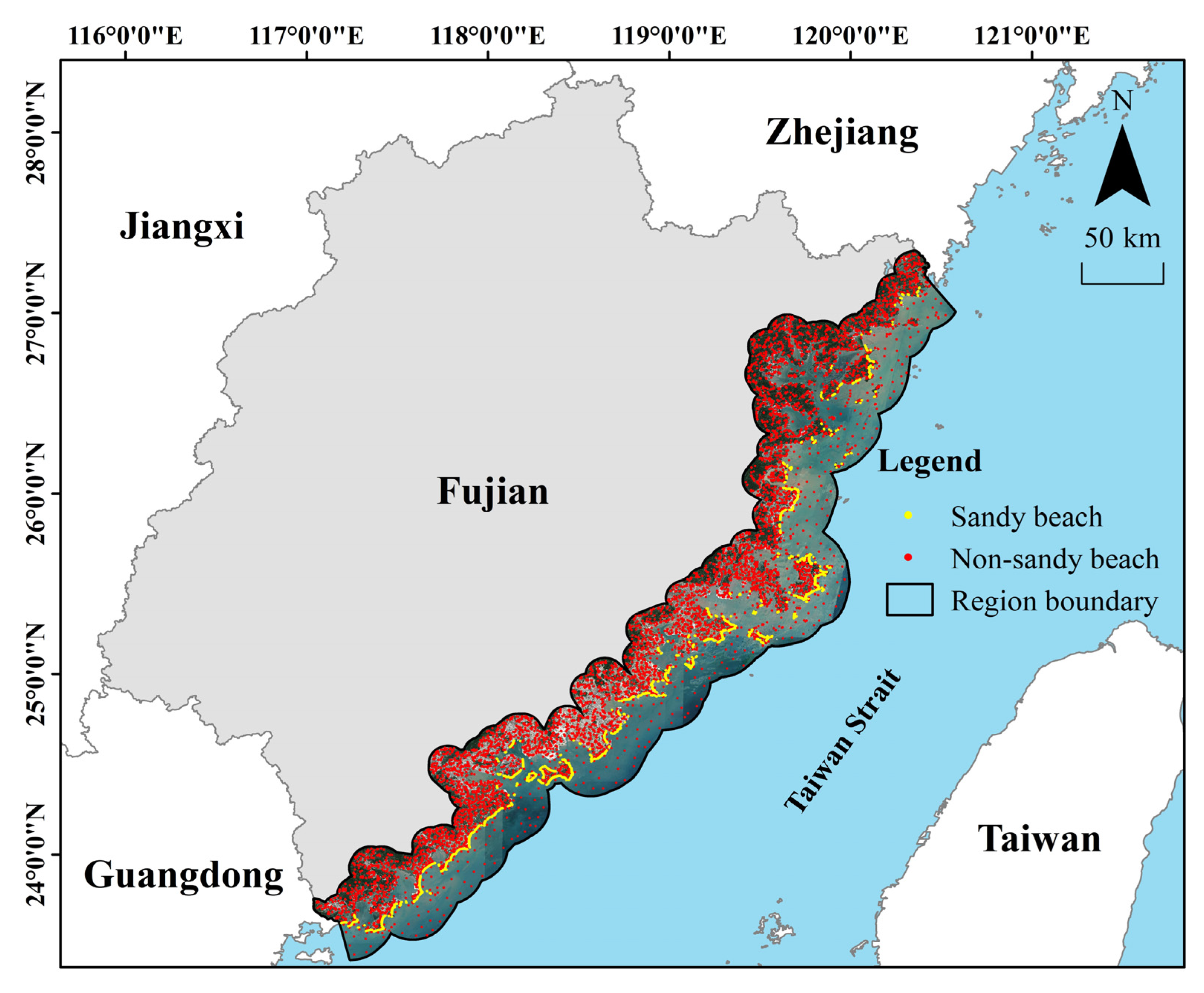
Figure 1. Geographical location of the study area.
Remotesensing 17 02754 g001
Figure 2. Technical framework of the study.
Remotesensing 17 02754 g002
Figure 3. Beach extraction performance of each model under different feature combinations.
Remotesensing 17 02754 g003
Figure 4. Feature optimization, importance analysis, and accuracy comparison: (a) trends of F1-score with increasing iterations in different models; (b) feature importance distribution in the optimal feature subset for each model; (c) comparison of sandy beach extraction accuracy before and after feature optimization.
Remotesensing 17 02754 g004
Figure 5. Spatial distribution and morphological characteristics of sandy beaches in Fujian Province: (a1d2) spatial distribution of sandy beaches in four representative regions; (e,f) frequency histograms of sandy beach area and perimeter in Fujian Province; (g) overall spatial distribution of sandy beaches in Fujian Province.
Remotesensing 17 02754 g005
Figure 6. Quantity distribution of feature types in the optimal feature subsets.
Remotesensing 17 02754 g006
Figure 7. Importance contributions in the optimal feature subset.
Remotesensing 17 02754 g007
Figure 8. Comparison of sandy beach extraction results: (a) comparison of sandy beach attributes; (b) comparison of sandy beach spatial distribution.
Remotesensing 17 02754 g008
Table 1. Candidate feature variables for sandy beach extraction.
Feature TypesFeature FactorsCalculation MethodsReferences
Spectrum Features (S)B2, B3, B4, B5, B6, B7, B8, B8A, B11, B12Based on the preprocessed Sentinel-2 data, specific bands were selected.Yin et al. [26]
Index Features (I)Normalized Difference Vegetation Index (NDVI)(B8 − B4)/(B8 + B4)Zheng et al. [27]
Normalized Difference Snow Index (NDSI)(B3 − B11)/(B3 + B11)Xiao et al. [28]
Normalized Difference Built-up Index (NDBI)(B11 − B8)/(B11 + B8)Muhaimin et al. [29]
Enhanced Vegetation Index (EVI)2.5 × (B8 − B4)/(B8 + 6 × B4 − 7.5 × B2 + 1)Wang et al. [30]
Soil-Adjusted Vegetation Index (SAVI)1.5 × (B8 − B4)/(B8 + B4 + 0.5)Xu et al. [31]
Bare Soil Index (BSI)((B4 + B11) − (B8 + B2))/((B4 + B11) + (B8 + B2))Ni et al. [32]
Normalized Difference Urban Index (NDUI)(NTL − NDVI)/(NTL + NDVI)Zhang et al. [33]
Vegetation Index (VI)((B11 − B8)/(B11 + B8)) × ((B8 − B4)/(B8 + B4))He et al. [34]
Land Surface Water Index (LSWI)(B8 − B11)/(B8 + B11)Chandrasekar et al. [35]
Modified Normalized Difference Water Index (MNDWI)(B3 − B11)/(B3 + B11)Tellman et al. [36]
Normalized Difference Tillage Index (NDTI)(B11 − B12)/(B11 + B12)Fernández-Buces et al. [37]
Ratio Vegetation Index (RVI)B8/B4Li et al. [38]
Difference Vegetation Index (DVI)B8 − B4
Modified Soil-Adjusted Vegetation Index (MSAVI)((2 × B8 + 1) − (((2 × B8 + 1)2 − 8 × (B8 − B4))0.5)2)/2Zhang et al. [39]
Enhanced Water Index (EWI)((B3 − B11)/(B3 + B11)] + ((B3 − B8)/(B3 + B8)) − ((B8 − B4)/(B8 + B4))Wang et al. [40]
Beach Morphology Index (BMI)(B112 − B8)/(B112 + B8)Wang et al. [41]
Polarization Features (P)VV, VHBased on the preprocessed Sentinel-2 data, specific polarization modes were selected.Jiang et al. [42]
VVVH_RIVV/VH
VVVH_DIFFVV − VH
VVVH_SUMVV + VH
VVVH_NOR(VV − VH)/(VV + VH)
Texture Features (T)Angular Second Moment (ASM), Contrast, Correlation (CORR), Dissimilarity (DISS), Entropy (ENT), Inverse Difference Moment (IDM), Sum Average (SAVG), Variance (VAR)The grayscale image calculated using the formula 0.3 × B8 + 0.59 × B4 + 0.11 × B3 was used to extract texture features of the study area with the help of built-in functions in GEE.Wang et al. [43]
Terrain Features (Tr)Elevation, Hillshade, Slope, AspectBased on the preprocessed terrain data, terrain factors of the study area were extracted using built-in functions in GEE.Lin et al. [44]
Table 2. Parameter settings of classification models.
Model NameModel Parameters
RFn_estimators = 100, random_state = 42
XGBn_estimators = 100, random_state = 42
LGBMn_estimators = 100, random_state = 42
GBMn_estimators = 100, random_state = 42
AdaBoostn_estimators = 100, random_state = 42
CatBoostn_estimators = 100, random_state = 42
Table 3. Performance evaluation metrics.
Metric NameCalculation Methods
Accuracy(TP + TN)/(TP + TN + FP + FN)
PrecisionTP/(TP + FP)
RecallTP/(TP + FN)
F1-score2 × TP/(2 × TP + FN + FP)
Table 4. Accuracy assessment of each model.
Model NameAccuracyPrecisionRecallF1-Score
RF0.96720.97050.95950.9647
XGB0.97430.97170.97330.9726
LGBM0.97430.97240.97330.9727
GBM0.97040.96660.96830.9683
AdaBoost0.96060.95330.96160.9581
CatBoost0.97390.97020.97410.9721
Stacking0.97500.97330.97250.9734
Disclaimer/Publisher’s Note: The statements, opinions and data contained in all publications are solely those of the individual author(s) and contributor(s) and not of MDPI and/or the editor(s). MDPI and/or the editor(s) disclaim responsibility for any injury to people or property resulting from any ideas, methods, instructions or products referred to in the content.